Submitted:
12 April 2024
Posted:
02 May 2024
You are already at the latest version
Abstract
Aquifer karstic structures, due to their complex nature, present significant challenges in accurately mapping their intricate features. Traditional methods often rely on invasive techniques or sophisticated equipment, limiting accessibility and feasibility. In this paper, we propose a new approach to non-invasive, low-cost 3D reconstruction using a camera that observes the light projection of a simple diving lamp. Our method capitalizes on the principles of structured light, leveraging the projection of light contours onto the karstic surfaces. By capturing the resultant light patterns with a camera, we reconstruct three-dimensional representations of the structures. The simplicity and portability of the equipment required make this method highly versatile, enabling deployment in diverse underwater environments. We validate our approach through extensive field experiments conducted in various aquifer karstic settings. The results demonstrate the efficacy of our method in accurately delineating intricate karstic features with remarkable detail and resolution. Furthermore, the non-destructive nature of this technique minimizes disturbance to delicate aquatic ecosystems while providing valuable insights into the subterranean landscape. This innovative methodology not only offers a cost-effective and non-invasive means of mapping aquifer karstic structures but also opens avenues for comprehensive environmental monitoring and resource management. Its potential applications span hydrogeological studies, environmental conservation efforts, and sustainable water resource management in karstic terrains worldwide.
Keywords:
Structured light method
; active 3D reconstruction
; cone estimation
; underwater karst aquifer
1. Introduction
Access to water has become one of the most pressing challenges facing humanity today. Yet water is abundant on a global scale: the oceans are an inexhaustible reserve, provided that salt and water are separated. Unfortunately, desalination methods are still too energy-intensive to be used profitably on a large scale. Pending a possible scientific breakthrough, we are therefore relying essentially on freshwater resources, which account for 2.5% of the world’s water [1] (Figure 1).
Only 1.2% of this freshwater is accessible at the surface, although it is now very polluted. Of the remainder, 68.7% is trapped in glaciers and ice caps and 30.1% is found underground. This groundwater, which represents 0.76% of the world’s resources, is extremely valuable. Groundwater is the result of a long and natural process of filtration through the various layers of soil, which means that its quality is generally considered to be very good. This groundwater is stored in aquifers, most of which are karstic.
Aquifer karstic structures, due to their complex and porous nature, present significant challenges in accurately mapping their intricate features. Traditional methods often rely on invasive techniques or sophisticated equipment, limiting accessibility and feasibility. In this paper, we propose a novel, non-invasive approach utilizing structured light projection in conjunction with a camera and a diving light to effectively map aquifer karstic formations. First part presents the main methods in underwater mapping. Second part details materials and methods of our original approach based on the principles of structured light, leveraging the precise projection of light contours onto the karstic surfaces. By capturing the resultant light patterns with a camera, we reconstruct detailed three-dimensional representations of the subsurface structures. Third part presents results to validate our approach by simulation of an aquifer galley first and finally through extensive outdoor experiments conducted in a particular equivalent aquifer karstic environment : The results demonstrate the efficacy of our method in accurately delineating intricate karstic features with remarkable detail and resolution. Furthermore, the non-destructive nature of this technique minimizes disturbance to delicate aquatic ecosystems while providing valuable insights into the subterranean landscape. This innovative methodology not only offers a cost-effective and non-invasive means of mapping aquifer karstic structures but also opens avenues for comprehensive environmental monitoring and resource management. Its potential applications span hydrogeological studies, environmental conservation efforts, and sustainable water resource management in karstic terrains worldwide.
2. Main Methods
Underwater mapping is a valuable tool in a wide range of applications, including marine biology, geology, archaeology, and the offshore industry. Various methods and sensors are employed to obtain 3D reconstructions of the environment, with data typically collected by divers, ROVs, or AUVs. In most cases, this involves performing surveys with downward-facing sensors and reconstructing the seafloor surface. The studies conducted by [2,3] provide comprehensive reviews of the various underwater 3D reconstruction methods. This synthesis of methods is illustrated in Figure 2.
Sensors used for 3D reconstruction can be classified into two main categories:
- active sensors: these sensors physically interact with the environment by emitting a signal or wave, such as sound waves in the case of sonars or light waves in the case of lidars.
- passive sensors: these sensors do not modify the environment, and the most commonly used ones for 3D reconstruction are camera-based.
Time-of-flight methods are the most direct methods for 3D reconstruction. They work on the same principle as a rangefinder: emitting a signal or wave and retrieving its echo. Knowing the speed of the signal thanks to the nature of the wave and the propagation medium, it is possible to proportionally deduce the relative distance between the sensor and the observed element from the measurement of the time elapsed between the emission of the wave and the return of the echo.
Among time-of-flight methods, those based on acoustic waves are by far the most used because their propagation is favored by the medium. They offer an interesting coverage capacity in front of the size of the areas to be studied in underwater mapping.
In addition and to allow the localization of 3D data during the measurement, most underwater navigation algorithms are based on acoustic positioning systems such as Doppler Velocity Log (DVL) and Ultra-short baseline (USBL) [4,5]. Multibeam sonars (MBS) are on the other hand adapted to bathymetric mapping (measurement of the seabed relief) [6] but much less to structured (non-flat) environments such as karst aquifers.
[7,8] presents a 3D model of the Zacaton cenote (a water-filled cave at least 300 meters deep) using sonar data collected by the DEPTHX (Deep Phreatic THermal eXplorer) vehicle. It is a NASA autonomous underwater vehicle measuring just over 2m and weighing over a ton, prefiguring among the robots that could explore underwater environments on other planets. Its sensors consist of a DVL, a sonar, an IMU and its movements are ensured by six motors allowing it to move in all directions.
Another method using acoustics is described by [9], which shows the results of an AUV performing limited penetration, inside an underwater cave using a mechanically scanned imaging sonar (MSIS for mechanically scanned imaging sonar). The results, obtained only for localization, show that it is possible to use this type of technology in our karst environment.
Efficient for obtaining bathymetry and macro-characteristics of habitats, these sensors nevertheless provide little information on fine characteristics (micro-bathymetry), do not allow to recover the texture of the environment and are very expensive.
Still in the class of time-of-flight methods, those based on electromagnetic waves, such as LiDAR, offer access to a very dense reconstruction of the seabed. However, on the other hand, they are reserved for very local observations, because the propagation of these waves are limited by the medium as we explained in the constraints. They are therefore not adapted to our situation.
The other class of methods is the triangulation method that we favor. These methods require at least two devices (or 2 different views) which will provide distance information from the same point, and thus form a triangle between the 2 devices and the point to be measured.
There are several ways to perform this triangulation, including:
-
Multi-view triangulation involves taking multiple views of the same scene. By knowing the disparities of each viewpoint, it is possible to project the points of the scene onto different "image" planes, and thus triangulate the points of the scene to obtain a depth map. This technique is based on epipolar geometry explained in [10] with two possible approaches:
- -
- the use of a binocular stereo system where the relative positions of the two cameras are known. It is possible to make the system active, by using a structured light projector to add discriminant points or features related to the observed environment and thus facilitate the matching of points between the two images for triangulation.
- -
- the method known as Structure from Motion (SfM) involves taking a sequence of sequential images of an object or scene, typically from a single camera. To obtain a metric reconstruction, it is necessary to know the camera trajectory to resolve the scale ambiguity.
- structured light triangulation relies on an emitter-receiver system. The emitter is a light source (laser or not) that projects a pattern (distinctive patterns) onto a scene observed by the receiver, a camera. Using the positions of the camera and the projector, it is possible to triangulate the discriminant points brought by the light in the scene captured by the camera [11].
Regarding structured light triangulation methods, they are very accurate, but are generally only used to reconstruct small areas or objects. This is because light is quickly absorbed in water; therefore, we must be close to the target to best detect the projected light. Additionally, structured light sensors are not yet well suited for mobility and are therefore mostly used statically for the moment.
Cameras, on the other hand, have the advantage of being inexpensive, providing dense data as well as texture. However, most camera-based methods operate in open areas with natural lighting (or with artificial lighting that completely illuminates the workspace) and generally try to reconstruct the ground or small objects.
For example, [12,13] propose a 3D reconstruction method based on a stereo pair for archaeological objects in shallow water and in very poor conditions. Special filters are implemented to solve the noise problems caused by these poor conditions. This static 3D measurement is fused with a 3D map of the excavation area obtained using a scanning sonar. [14] performs a dense reconstruction of submerged structures at very high depths (up to 6000 meters) with a stereo system mounted on a controlled manipulator arm. The imposition of a known trajectory allows to know the different positions of the cameras to calculate a precise 3D model of the scene.
[15] reconstructs coral reefs with a wide-baseline stereo system using high-resolution video and a dense reconstruction method.
Our context is different from these works since we are in total darkness in a structured and extended environment whose content appears as the diver or robot moves.
[16] presents a description of the problems related to metrology in the underwater environment. The importance of calibrating the stereo pair underwater is emphasized, taking into account the refraction problems related to the medium. The detection of interest points is done on sufficiently bright images allowing a robust matching then used for a 3D reconstruction. The comparison of the object measurements obtained is made with a reference metrology and gives good results but in statics.
The work of [17] is directly related to our theme. The objective is to reconstruct a karstic underwater tunnel of Woodville Karst Plain in Florida using a new approach to stereovision generating a 3D point cloud of the cave. In their method, after calibration and rectification of the highly distorted images, they extract the contours of the artificial light projected into the cave which creates a cone of light illuminating part of the walls. These contours are then used as inputs in their stereovision algorithm. The displacement is estimated by visual odometry (ORB-SLAM) and allows a 3D reconstruction of a portion of the cave of about one hundred meters but without specifying the comparison of the result with a known ground truth.
For an even more optimal mapping of this underwater gallery, [18] have developed a SLAM method where they fuse this stereo method with a sonar and an inertial measurement unit, thus improving the accuracy of their measurements.
[19] uses a SFM method coupled with multi-view stereo photography to perform measurements of silting areas at the outlet of water transport pipelines to the seabed. The accuracy of their method allows a robust estimation of these elements useful for monitoring these areas but also remains static measurement.
[20] provides an overview of calibration and underwater image processing methods in structured light. [21] proposes a method of 3D reconstruction in underwater environments combining a SLAM approach and dense reconstruction using a stereo system embedded on the Aqua2 robot whose IMU allows localization. The results are mainly on coral reefs and partially on the reconstruction of underwater cavities. The question of the accuracy of the measurements with respect to a ground truth remains. [22] proposes an application of 3D reconstruction for underwater archeology. The system consists of two monochrome cameras and a sinusoidal light pattern projector. A combination of 3D reconstruction in structured light and SLAM-based visual odometry is proposed. All mounted on an ROV whose IMU data complements that of visual odometry. The first results are obtained on objects in a controlled environment. A test is then carried out over a dozen meters to follow a pseudo pipeline. But the size of the system is too large for an application in underground galleries.
[23] uses Ariane’s thread to enable the movement and guidance of a BlueRov robot. This learning method gives good results for localisation and assisted piloting. The next steps envisaged are autonomous navigation and then mapping of the cavities studied (but already explored by divers).
[24] proposes a real-time monocular 3D reconstruction method for underwater environments. It relies on optical flow tracking of characteristic seabed points and uses Delaunay triangulation to complete the seabed estimation. The method assumes a nearly planar seabed but remains unclear about the achieved metric accuracy.
3. Materials and Methods
The complete development of our method is detailed in Figure 3 and is based on three main blocks :
- calibration of the camera is used to estimate its intrinsic parameters, including radial distortion,
- calibration of the projector consists of estimating the geometric parameters of the cone (vertex , direction , half-angle of opening ),
- local 3D reconstruction based on the camera / projector triangulation leading to a 3D point cloud expressed in , the camera frame.
This triangulation is illustrated in Figure 4. It shows our system, with one camera and light projector. To simplify the figure, the light is projected onto a plane, but you can imagine that the procedure has to be applied to non-planar surfaces such as the walls of a gallery. Once the light contour has been detected in the image, the associated camera ray is calculated for each point on the contour. The Figure 4 shows two points and belonging to the contour detected in the image and the rays associated with them. In the configuration shown in the Figure 4, the ray associated with (respectively ) intersects the cone at two points and (respectively and ). To calculate these intersections we need to know the angle of aperture and the transformation between the references of the cone and the camera called .
Still on the Figure 4, the intersections which correspond to the 3D points of the contour ( and ) are shown in green and those which should not be taken into account () are shown in red. The point is not shown, but we can imagine that it would be red and beyond the area of the plane in the Figure 4. For a given ray, it is therefore necessary to identify whether it is the first intersection or the second intersection that belongs to the observed light contour.
This method of selecting intersections requires a study of the geometric relationships between the cone and the camera.
3.1. Cone Parameters
3.1.1. Cone of Revolution
The cone of revolution, referred to as a cone in the remainder of this document, is associated with its surface of revolution and not with its solid, as may be the case in certain applications. The terms we will use to define the relationship between a point and the cone are as follows:
- a point belonging to the cone is a point which belongs to the surface of the cone,
- a point inside the cone is a point which belongs to the solid bounded by the surface of the cone,
- a point outside the cone is a point which does not belong to the solid bounded by the surface of the cone.
This surface is generated by the revolution of a line, called the generatrix, which we will note g and which passes through a vertex, in this case .
The revolution takes place around a fixed axis which also passes through the vertex and which turns out to be an axis of symmetry of the cone, the direction of which is defined by the unit vector .
If a plane not passing through is orthogonal to the axis of symmetry, then its intersection with the cone is a circle.
Thus, the angle formed by g and the axis of symmetry is constant and corresponds to the half-angle of the cone opening .
The cone is represented in Figure 5 with the orthonormal base , oriented such that , which defines the reference frame associated with the cone.
The generatrix g has the unit direction vector which is set by a new angle (Figure 5).
In the cone frame , we can simply express the vector which then depends only on the angles and :
This vector can be used to express all the points on the surface parametrically.
Let be a point expressed in the reference frame . Then, if belongs to the cone we have :
with l a real parameter whose absolute value defines the distance between and the cone vertex. However, with , the parametric equation defines a "double cone". However, since the cone models our light projector, we are only interested in the upper part of the "double cone", i.e. when the parameter .
3.1.2. Orthogonal Distance
This parametrisation of the cone will help us to write the equation for the orthogonal distance between a point and the cone, an equation that will be useful for cone estimation.
Let be a point outside the cone and its orthogonal projection on the cone (see Figure 5).
The angle is the angle that gives the generatrix of the cone closest to . This generatrix, called , passes through and has the unit direction vector whose expression in the reference frame is :
If we also express in with , we obtain the following expressions:
If then the projected point is in the lower part of the cone. As we are only working with the upper part of the cone, when this condition is true, the nearest point is the vertex of the cone (see example Figure 6). The orthogonal distance h is therefore :
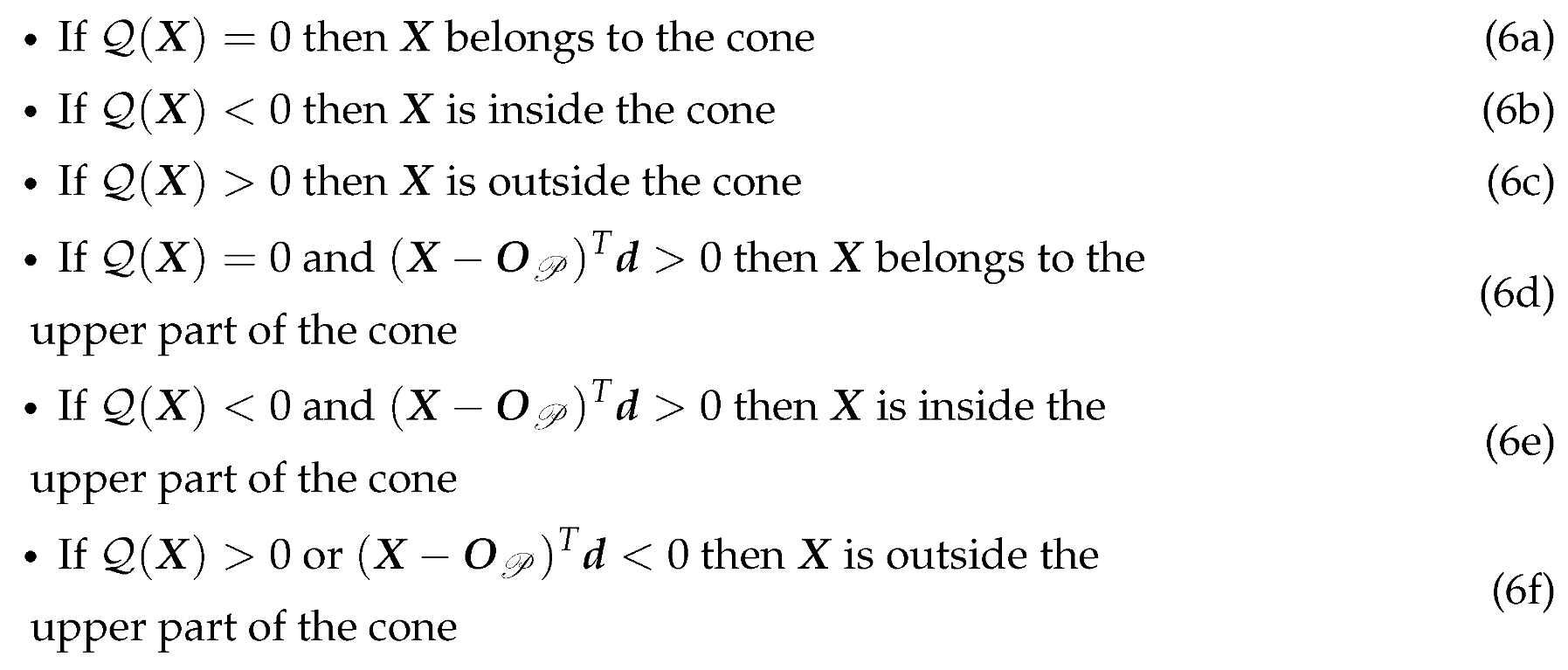
3.1.3. Quadratic form of the Cone
To obtain this relationship, we must first note that if the angle between the vectors and or and is equal to the angle , then the point belongs to the cone. This is equivalent to the following scalar product:
When squared, the expression becomes :
We thus obtain a quadratic function of the cone in the general case, directly showing the parameters , and which define it:
This gives the relationships between the point and the cone:
3.2. Projector Calibration
Projector calibration is an essential step, since it involves estimating the parameters of the cone used in our method and in the equations we have seen so far. As a reminder, the parameters of the cone to be estimated are its vertex , its direction vector and its half-angle of aperture .
Since and represent the relative pose of the cone with respect to the camera, the projector must be fixed with respect to the camera during calibration and during any experimentation. Furthermore, if the projector has a variable half-angle aperture, it is also necessary to ensure that this is fixed.
3.2.1. 3D Point Generation for Cone Estimation
The first step in the calibration method is to generate a cloud of 3D points belonging to the cone. To achieve it, the chosen method is to capture several light projection images on a flat surface.
This light projection is the result of the intersection between the projector cone and the flat surface, which is by definition a conic. In our case, it will be an ellipse because we want a closed shape. The projection of this ellipse into the image is also an ellipse.
If we can estimate the relative pose of this surface with respect to the camera and extract the light contour in the image, which is an ellipse, then we can obtain the real ellipse from the ellipse in the image.
To estimate the relative pose, we attached a chessboard pattern to the surface to estimate its relative pose. This relative pose is obtained by estimating the homography between the calibration pattern and the image plane [25]. As the camera is calibrated, rotation and translation can be estimated from the homography.
To extract the ellipse from the image, we again use the contour detection method presented in [26,27].
Then, from the contour points obtained, we estimate the best ellipse using the method of [28] which is based on least squares optimisation.
It is therefore possible to obtain n elliptical sections of the cone from n images taken at different distances from the surface. For each ellipse extracted in an image, we obtain the ellipse in the surface via the estimated homography between the image plane and this surface. The estimated relative pose allows us to obtain the elliptical section, i.e. the set of 3D points expressed in the camera frame of reference belonging to the ellipse of the surface.
Figure 8 shows an example where the camera has captured three images of an ellipse surrounding a chessboard pattern on the flat surface in three different poses. This is equivalent to obtaining three elliptical sections of the same cone.
Figure 7.
Example of detecting the contour of a halo of light on a wall using a chessboard to estimate the plane pose. The contour is in green and the adjusted ellipse in blue.
Figure 7.
Example of detecting the contour of a halo of light on a wall using a chessboard to estimate the plane pose. The contour is in green and the adjusted ellipse in blue.
Consequently, if we have obtained n elliptical sections where m 3D points are extracted per section, we generate a cloud of 3D points belonging to the cone.
3.2.2. Cone Estimation
The aim is now to estimate the cone that best approximates the 3D point cloud. This is done by geometric fitting, i.e. by minimising the orthogonal distances between the 3D points and the cone.
Let be the vector containing the six parameters of the cone, which are :
- the three coordinates of its vertex ,
- the two angles yaw and pitch in ZYX-Euler convention of its direction vector , the angle roll not being necessary since a cone has an axis of symmetry,
- its opening half-angle .
To estimate the vector, we use the Levenberg-Marquardt (LM) iterative method [29]. For the first iteration, we need to choose an initial parameter vector . This could be the null vector, for example. In practice, we will use measurements taken with a caliper for the various parameters of .
At each iteration i, LM receives a solution vector and the function for calculating the vector of orthogonal distances to be minimised. Our function first calculates the rotation and translation of the cone relative to the camera from and the yaw and pitch angles of the vector . It then expresses the 3D points in the cone reference frame and calculates the orthogonal distance vector between the 3D points and the cone using the equation 4.
So from and this function, LM returns a new solution vector .
When the difference between the sum of the squared orthogonal distances obtained with and the calculus obtained with is less than an arbitrary threshold, this means that LM has reached convergence at iteration j. The best solution in the least squares sense is therefore the vector .
It is important to note that there are an infinite number of cones that share the same elliptical section. On the other hand, there is only one cone that passes through an elliptical section and through a point outside that section. Consequently, this minimisation can only work if we have at least two elliptical sections.
3.3. Intersection with a Ray
Now that we know how to determine the cone parameters using our calibration method, the next step is to be able to calculate the intersections between a camera ray and the cone. We are only interested in the intersections with the top of the cone.
A ray is a half-line that can be expressed parametrically using the following equation:
with the starting point of the ray, its unit direction vector and t a positive real number such that . Note that we will only deal with cases where the point is outside the cone. This is because the starting point of the camera rays is the optical centre in our situation. The point can nevertheless be inside the lower part of the cone.
If is an intersection point, then it belongs to the cone. Therefore, to determine the intersections, we can simply calculate the values of t which cancel the general polynomial of the cone (see 5) after replacing by the expression for :
3.4. Projection of the Generatrices of the Cone in the Image
To understand the relationship between a point on the cone and its projection into the image, we need to look at the projections of the generatrices of the cone. Since the cone represents the projector, we will only consider the upper half of the cone, which means that the generatrices can be limited to the half-lines that start at the vertex . Note that the study is limited to the case where the cone is oriented in the same direction as the camera, as required by our method. Geometrically, this condition is satisfied if the angle called between and is in the interval ][ (see Figure 9). In practice, for the camera to be able to see the light projection, the angle will be close to 0.
3.4.1. Calculating the Projections of the Generatrices of the Cone
Let us call the plane which passes through the optical centre and through at least one generatrix of the cone. The intersection of this plane with the image plane is the line .
Let be a point in the image such that with the direction vector of the camera ray associated with . If is the projection into the image of a 3D point belonging to a generatrix resulting from the intersection between the cone and the plane , then belongs to the line . However, if belongs to the line , it is not necessarily the projection of a point on the cone. To obtain the equation of , the simplest way is to select two points belonging to one of the generatrices (or the generatrix) through which the passes, then project them into the image to find the parameters of the line. The same result would be obtained by projecting two points of the plane which do not belong to the same camera radius. However, knowing the line is not enough to understand the projection of a generatrix.
Observation When Is Not Tangent to the Cone
When the plane is not tangent to the cone, it passes through two generatrices and , with chosen as the generatrix closest to the optical centre (see Figure 10).
The direction vectors of these two generatrices are and such that :
with (respectively ) the angle between the vector (respectively ) projected in the plane and the vector (see Figure 10). As the plane is chosen here as not tangent to the cone, we have . In this configuration, if is a point on the line then it can be both the projection of a point belonging to and of a point belonging to . The generatrix therefore contains the first intersections of the camera ray with the cone, while contains the second intersections.
Calculating the Two Special Generatrices When Is Tangent to the Cone
There are only two orientations for which the plane is tangent to the cone. When this happens, then and the generatrices and are superimposed. The two possible cases are illustrated in Figure 11. The two angles and define the two generatrices and through which pass the two planes tangent to the cone and . It is important to note that the angles and depend solely on the parameters of the cone and its pose relative to the camera , which means that they are unique and fixed for a given configuration.
To determine these two angles, we will use a plane tangent to the cone called which passes through a generatrix g whose direction vector is defined by an angle . It is represented in Figure 10 passing through the generatrix purely for reasons of visibility. The orientation of the plane is characterised by the unit normal vector such that :
We are therefore looking for the two solutions of so that the plane is superimposed on the plane or . This superposition only occurs when the plane passes through the optical centre and therefore when the vector is orthogonal to the vector ( - ). We are therefore looking for when :
with the optical centre expressed in the reference frame of the projector. To solve the equation 9 we pose :
We can rewrite the equation 9 using the scalar product between the vectors and and the angles defined in Figure 12 :
The angle between the vectors and is therefore :
As for the angle which defines the orientation of the vector , its expression is :
The solution to equation 9 is therefore :
Note that the two angles and only depend on the half-angle of the opening of the cone and the translation between the cone and the camera (translation expressed in the equation by ). From the expression of these two angles, we can obtain the expression of the two unit direction vectors and of the two special generatrices and . The projections of these two generatrices belong to the lines and which are the intersections of the image plane with the planes and .
Splitting the Cone into Two Areas Using the Two Special Generatrices
Using the generatrices and we can divide the cone into two surfaces as shown in Figure 13. The cyan surface named (resp. magenta surface named ) contains the set of generatrices containing all the first (resp. second) possible intersections between a camera beam and the cone, generatrices previously named (resp. ).
In the image plane, this shows that we can delimit the areas where the camera rays can intersect the cone. The cyan area, surrounded by the ellipse , contains the projections of part of the set of 3D points belonging to the surface . The magenta area contains the projections of the other part of the set of 3D points belonging to the surface and contains the projections of the set of 3D points belonging to the surface . These areas are bounded by :
- the lines and .
- the ellipse which is the set of vanishing points of the generatrices. These points define a first bound on all the projections of the generatrices.
- the projection of the vertex into the image plane, named . It defines a second bound on all the projections of the generatrices.
In the configuration illustrated in Figure 13, each generatrix projection is therefore a segment whose limits are the vanishing point of the generatrix belonging to the ellipse and the point .
However, there are other configurations where the projections of the generatrices onto the image plane are not segments but lines. Indeed, if , then the line passing through and is parallel to the plane, which implies that the projection of the vertex into the image plane is a point at infinity (or ideal point) and that the lines and are parallel.
The case where is illustrated in Figure 14 which shows the lower part of the cone behind the camera. This part is shown in brown and its projection in the image plane is also in brown. This projection is obviously fictitious, as this part cannot be seen by the camera even if it had an infinite field of view. The point , also fictitious, is still the intersection of the lines and , but this time it is on the other side in comparaison of the Figure 13.
As for the magenta and cyan areas in the image plane, they are still delimited by the lines and and the ellipse but extend towards infinity on the side where the lines and diverge.
So if then each generatrix projection is a half-line whose only boundary is its vanishing point belonging to the ellipse . However, as we are working with real cameras and not with the image plane, which is infinite, each generatrix will have a segment as its projection into the image.
This division of the cone into two surfaces leads to several results:
- Any ray associated with a point in the cyan area has as its unique intersection with the cone a 3D point belonging to the surface .
- Any ray associated with a point in the magenta area has two intersections with the cone, the first of which belongs to the surface and the second to the surface . These two intersections are superimposed if the point in the magenta area belongs to the line or to the line .
- Any ray associated with a point outside the magenta area and the cyan area does not have any intersection with the cone.
3.5. Intersection Selection and Triangulation
We now have everything we need to develop a method for determining which intersection to choose when the ray associated with a pixel in the contour has two intersections with the cone. To better understand the various stages of the procedure, let’s take as an example the 3D contour of light whose associated 3D curve is circular and results from the intersection between a plane and the cone.
The example of the circular contour is illustrated in Figure 13 which contains the following elements:
- is the closed 2D curve corresponding to the contour in the image with a 2D point on the curve.
- is our circular 3D curve corresponding to the contour of the light in the scene, with a 3D point on the curve which has as its projection. The point therefore corresponds to the correct intersection between the cone and the camera ray associated with .
- The areas containing the first and second intersections with the cone are delimited by the two generatrices and which divide the cone into two surfaces and . They also divide into two curves, one in cyan called and the other in magenta called .
- and are respectively the two intersections of and with the curve and are thus the only two 3D points common to the curves and .
- The cyan curve named and the magenta curve named are respectively the projections of the curves and .
- and are the projections of and and are therefore the only two points common to the curves and . They belong to both the curve and the lines and . So, in theory, they correspond to the two unique points of tangency of the lines and with .
So, if we get the points of tangency and , we will be able to divide the 2D curve in two via the line . However, in practice :
- the curve is discrete,
- the light contours are extracted in a perfectible way,
- the camera calibration and the cone estimation have uncertainties, so the lines and also have uncertainties.
All this means that the lines and are not exactly tangent to the curve . The method for determining the points and must therefore be adapted to this constraint.
Once these two points have been obtained and the curve has been divided in two, it remains to determine which of the two curves is or . To do this, we need to look at the relative position of the vertex in relation to the camera. Figure 15 shows that the vertex and the curve lie in the same half-space bounded by the plane passing through and the line . This property is always true whatever the pose of the cone.
In the image plane, this property can be expressed by defining a point such that and the curve lie in the same half-plane bounded by the line .
There are an infinite number of solutions for in the image plane which satisfy this condition. We have therefore forced to belong to the circumscribed circle of the rectangle delimiting the image, as can be seen in Figure 15. The segment between and the centre of the image forms an angle with the horizontal axis of the image called . This gives :
with w and h respectively the width and height of the image in pixels. For the condition to be true, one possible solution for is to indicate the direction of relative to the optical centre . To obtain this angle, we orthogonally projected onto the plane normal to the camera axis passing through , which gives the point illustrated in Figure 15. This gives which is the angle formed by the vectors and :
Calculating this angle and the point allows us to deduce which of the two curves is .
Once the curves and have been obtained, it is then possible to obtain the 3D contour. Indeed, if a point belongs to , then the first intersection of the camera ray associated with it must be chosen, and if it belongs to , the second must be chosen. This is because any point of is the image of a 3D point of , and any point of is the image of a 3D point of .
3.6. Test of the Method in Simulation
Contour Simulation
To illustrate the different stages of the method, we will use a gallery model. Figure 16 shows the camera represented by a pyramid and the projector represented by a cone positioned inside our model. In our example, the axis of the cone is parallel to the axis of the camera. The vertex is positioned above and to the right of the camera ; it belongs to the plane which passes through the optical centre and which is orthogonal to the camera axis. Consequently, the projection of in the image plane is a point at infinity (an ideal point) and the projections of the generatrices all belong to lines parallel to each other.
The 3D curve is the intersection between the cone and the model. The set of 3D points on this curve is thus obtained from the intersections of the generatrices of the cone with the model, and they are shown in black in Figure 16. The number of 3D points is equal to the number of generatrices chosen to represent the cone. These 3D points are then projected onto the image to obtain a set of 2D points belonging to the curve . These 2D points are shown in black in Figure 16.
The idea now is to obtain the 3D points of the curve from the 2D points of the curve . We will assume that the parameters of the cone and the camera are known.
Calculating the Generatrices and the Lines Containing Their Projection
The first step is to calculate the direction vectors and of the generatrices and . To do this, we need to calculate the angles and using the equation 10.
Once the direction vectors have been obtained, we select two 3D points on and , project them into the image and compute the parameters of the lines and . The two lines are defined by their respective unit direction vectors and and by and , two points belonging respectively to the two lines.
Determining the Points and
We wish to obtain the points and which are theoretically the points of tangency of the lines and with the curve . We will only present the approach for the point since it will be the same for .
A first solution would be to say that is the point belonging to the line closest to the curve . However, we have chosen a slightly more generic approach, the result of which is illustrated in Figure 17. It consists of considering as the point belonging to the line which minimises the sum of the squared distances between itself and the x% of the points on the curve closest to the line . Let t be the parameter of the line. We are therefore looking for t such that :
Where :
- are the x% of the points on the curve closest to the line .
- is a function whose aim is to reduce the impact of the points far from the line in minimisation.
Figure 17 shows the points and obtained, with 40% of the points closest to in yellow and 40% of the points closest to in orange. Developing the sum to be minimised in 14 gives us :
avec
Since a must be positive, the polynomial has a minimum when its derivative cancels, i.e. when :
This gives :
Using the same procedure, we can obtain the point . This produces the line (see Figure 17) which will be used to divide the curve in two.
Separation of the Curve for Intersection Selection
The points and are determined in a perfectible way in reality. We have therefore defined a minimum distance around the line called e which the points of the curve must respect. Points whose distance orthogonal to the line is less than e are considered indeterminate and will therefore not be taken into account in the 3D reconstruction of the contour. In practice, the value of e will depend on the quality of the measurements taken.
This separation of the curve into two curves is illustrated in Figure 18 with in cyan and in magenta.
To obtain or , we had to use the point (see equation 12) obtained via the angle (see equation 13) and apply the following two conditions:
with , the normal vector to the line .
3D reconstruction
We now know which points on the curve belong to the curve or the curve . We can therefore apply what was presented in the Section 3.3 and Section 3.5 to reconstruct these points in 3D.
Figure 19 takes the 3D scene from Figure 16 and adds the reconstructed 3D points. The calculated differences between these reconstructed 3D points and the initial 3D points of our simulation (obtained via the intersection between the generatrices of the cone and the gallery model) are below m, which is very small. These deviations are due to numerical errors in the calculations at the various stages. This proves that these reconstructed 3D points are the same as the initial 3D points and that our method therefore works. We can now test the method with real data.
4. Experiments in a Waterless Aqueduct
The local heritage offers us access, between two of our laboratory buildings, to the Saint-Clément aqueduct (more commonly known as the Arceaux aqueduct) built in the 18th century. It is no longer in use, but in dry periods it is an ideal experimental platform. The gallery is accessible via trapdoors, which once closed plunge you into total darkness. This confined space recreates experimental conditions similar to those in a karstic environment, but in a dry environment whose dimensions are easy to measure. Indeed, the aqueduct is simply a long corridor whose left and right walls are parallel and separated by a width of 62cm, which we measured with a laser rangefinder.
4.1. Our System
The camera used is the Nikon D7000 reflex and we set it to a focal length of 18 mm and a resolution of .
The projector is the DIVEPRO M35 dive light with an aperture angle of in air and in water. As the aperture angle is too large to capture the full projection of light in our experiment, a custom-made plastic cylinder (obtained from the 3D printer) was added to reduce it, as can be seen in Figure 21. Its internal diameter is the same as the diameter of the projector, i.e. 53,8mm. The cylinder protrudes from the projector by mm (see Figure 20). We can therefore calculate the half-angle of aperture as a function of the lengths l and d :
We will use this value to check the order of magnitude of future values when we estimate the cone.
The camera and projector are placed on a rigid support as shown in Figure 21. They had to be fixed to the support because the slightest rotation of one in relation to the other alters the transformation between the camera and the projector, which is estimated during the projector calibration.
To get an idea of the magnitude of this transformation, we used a caliper to measure the translations between the camera and the projector along the camera’s x, y and z axes. The rotation between the two is supposed to be small because we have chosen an identical orientation for both. Here is a summary of the various measurements of the projector parameters (lengths in m):
4.2. Camera Calibration Results
To calibrate our camera, we use the method of [30] with the help of eight images of a flat chessboard test pattern measuring 7x10 squares and 36mm wide (see Figure 22). In each of the eight images, the position of the test pattern relative to the camera is different, as can be seen in Figure 23, which is a 3D representation of the test pattern in eight different positions. Here are the camera parameters estimated via calibration:
- the intrinsic matrix K obtained is :
- the resulting focal length is 18.2 mm,
It can be seen that the orders of magnitude of the various camera parameters are consistent with the manufacturer’s parameters. In addition, the average reprojection errors are of the order of 1/10 of a pixel. This level of error is quite satisfactory for all eight shots, each containing 56 calibration points.
4.3. Projector Calibration Results
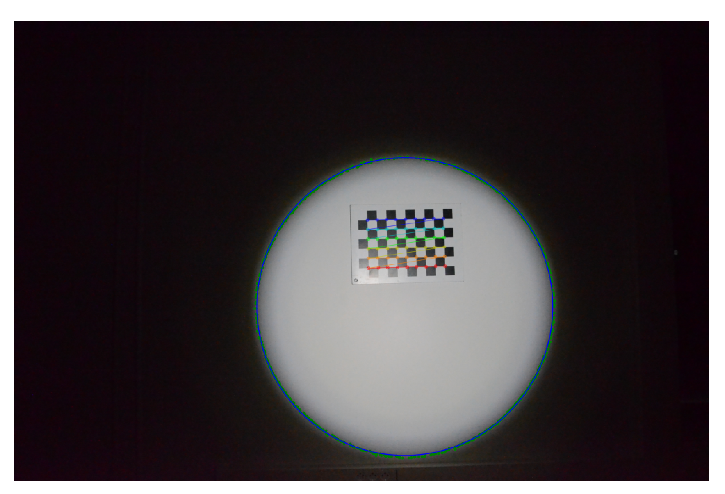
To calibrate the projector, i.e. estimate the parameters of the cone, we used a white wall on which a chessboard pattern was hung. The first step is to obtain 3D points belonging to the cone by detecting the contour of the light projected onto the wall, as explained in the section entitled 3.2. To maximise the contrast of the light projected onto the white wall, the only light source in the room is the projector.
For this calibration, we captured five images of light projected onto the wall with the axis of the cone almost orthogonal to the wall (see Figure 24). The shape of the projected light therefore resembles a circle.
Each detected contour is transformed into an ellipse, shown in blue in Figure 24. To obtain the ellipses we use the method detailed in [28] but iteratively with the RANSAC algorithm [31] to eliminate certain outlying contour points. The contour points eliminated by RANSAC are shown in red in Figure 24 while the points used to obtain the ellipses are in green.
Using the pattern detected in each image, we obtain the equations for the five planes. From these five planes and the five ellipses obtained, the five elliptical sections are calculated. They are represented in 3D in Figure 25 with the camera and the test pattern.
The image on the left shows all the elements expressed in the chessboard pattern frame, so you can see the different camera positions used to capture the five images.
The image on the right shows all the elements expressed in the camera frame. It is in this frame of reference that the elliptical sections must be expressed in order to estimate the cone.
We extract 3D points expressed in the camera frame of reference for each elliptical section. In our case, we recovered 200 points per section, making a total of 1000 3D points. Note that these 3D points are at a distance from the camera frame of between 1,50m and 2,17m.
Now that we have obtained 1000 3D points that are supposed to belong to the cone, the next step is to define an initial cone for our iterative minimisation algorithm. This is shown in red in Figure 26. We chose an initial cone that is far from the solution for greater visibility in the figure and also to prove that the method is capable of converging even when the initial cone is far from the solution. Obviously, this is an experimental result and not a mathematical proof. This optimisation problem is probably non-convex. Ideally, therefore, an initial cone close to the solution should be chosen using the aperture angle previously calculated and the relative pose measurement between the projector and the cone.
We therefore apply our algorithm and obtain the optimised cone shown in grey. Its estimated parameters (lengths in metres) are :
To ensure the validity of the cone obtained, we begin by comparing the estimated parameters with the previously measured parameters. The Table 1 compares the estimated opening angle and the estimated gap with the measurements. As our measurements can be improved, this comparison at least proves that the order of magnitude of the estimated parameters is consistent.
Another point to check is the minimisation error for estimating the cone. In our case, this error is directly linked to the orthogonal distances between the 3D points of the elliptical sections and the cone, since it is the root mean square (RMS) of these distances that we are trying to minimise during estimation. In Figure 26, the colour of each 3D point is defined by its orthogonal distance from the cone via the colormap Jet (the colormap bar is shown in the figure) and the following function :
with d the orthogonal distance. m is chosen as the median of all these distances (here mm).
The statistics for these distances can be found in the Table 2. In particular, we have a maximum distance of 4,2mm and an overall mean of 1,5mm. The overall RMS is 1,9mm which corresponds to approximately 0,13% of 1,50m which is the smallest distance between a 3D point of an elliptical section and the camera frame.
In view of the analysis of the orthogonal distances, the minimisation is satisfactory, confirming once again that the estimated parameters of the cone are at least consistent with their true values.
4.4. 3D Results
The shape of our aqueduct is a long narrow corridor, which makes it possible to fully distinguish the light projection in our images. We captured six images taken at different distances from a chessboard pattern placed in the aqueduct. For each image, the light contours were checked manually, as we wanted to isolate the triangulation method from the contour detection method, which is still in need of improvement. For each contour extracted, we manually delimited part of the contour points on the left wall and another part on the right wall. These delimitations can be seen in Figure 27. It shows an example of an extracted contour in two images, with contour points on the left wall in red, on the right wall in blue and the rest of the contour points in green.
Only the contours of the left and right walls will be used for triangulation, as this will allow us to check that the 3D points obtained respect the dimensions of the aqueduct corridor. To obtain these 3D points, it is necessary, as usual, to define which intersection is relevant for each radius associated with the contour points. In our situation, we can see that each contour point on the left wall implies a first intersection and each contour point on the right wall a second intersection. Figure 28 illustrates this for the two images in Figure 27.
Figure 29 shows the result of the reconstruction of the contours of the six images. The shape of the 3D reconstructions of the contours is close to a hyperbola, which is consistent since the intersection between a plane and a cone in this configuration is supposed to be a hyperbola.
We’re now going to compare this 3D reconstruction with reality. The aqueduct is a corridor whose left and right walls are parallel and separated by a width of 62cm. We can therefore check that :
- the 3D points resulting from the left part (respectively right part) of the contour belong to the same plane so they are supposed to be coplanar,
- If we estimate a plane from the left 3D points and a plane from the right 3D points, they must be parallel and separated by a distance of approximately 62cm.
As shown in Figure 29b, we get estimations of the left wall in red and the right wall in blue by using a least square method. To evaluate coplanarity, we compute the deviation between 3D points and their associated plane. For left points, we get an average deviation of 13,9mm and for right points 24,1mm (see Table 4).
To check the gap between the two estimated planes, we compute the distances between the left 3D points (respectively the right 3D points) and the right plane (respectively the left plane). The average distance between the left points and the right plane is 584,9mm. The average distance between the right points and the left plane is 583,6mm.
The two estimated planes are almost parallel since the angle calculated between the 2 normal vectors is 178,9°.
5. Discussion
Authors should discuss the results and how they can be interpreted from the perspective of previous studies and of the working hypotheses. The findings and their implications should be discussed in the broadest context possible. Future research directions may also be highlighted.
6. Conclusions
The aim of this paper was to propose a 3D reconstruction solution designed for underwater galleries found in karstic environments. The study of these environments represents a considerable challenge for the future, as they could provide part of our water needs. Exploration remains the best approach for acquiring reliable data on the structure, and is mainly carried out by qualified divers using topography methods with Ariane wires and section-by-section surveys. But on extensive karstic networks, this approach presents a major risk, as the duration of these surveys is so time-consuming, leading divers to long stops. The future is therefore more likely to lie with robotics, but there are still many technical challenges to be overcome before underwater drones that are sufficiently autonomous can be sent out to explore this type of environment. Our aim was to propose an original method of 3D scanning in this type of environment. Our approach uses a combination of a camera and a cone-shaped projector. The parameters of the light cone have been fixed: its centre, its direction vector and its angular aperture. A method for calibrating the cone was presented, enabling the position of the 3D points obtained by intersecting the visual rays of the contour of the projector halo as seen by the camera with the cone whose parameters have been estimated. The calibration of the camera is done thanks to a classical approach. A simulation of this method was presented and results validate the proposal. A first experimentation in real conditions was conducted in a disused aqueduct (without water) which had the advantage of reproducing an environment close to that of a karstic aquifer: narrow, without light and above all without water to continue our evaluation. The camera calibration is validated with an error reconstruction less than 0.1 pixel and camera parameters close to technical values (see 4.2). The cone calibration leads to an angles error less than 2 degrees and distance with respect to the camera less than 2 mm. The results were validated by testing the coplanarity of the aqueduct walls to within 25mm and estimating the known distance between these walls to within 36mm (see Table 4). Experiments have be done in real karstic environment but due to complex meteorological conditions, visual acquisition was not possible. Thus, we aim to begin in a more controlled environment : a swimming pool and then finish in a real aquifer with clearer water.
To explore a new configuration of this system, we began to make some simulations with one projector and four cameras (Figure 30) to solve the error of the transition zone (see Figure 19). We also think about using several projectors with localisation sensors with respect to one or more cameras to have different configurations and measurement redundancy.
References
- Gleick, P.H. Water in crisis. Pacific Institute for Studies in Dev., Environment & Security. Stockholm Env. Institute, Oxford Univ. Press. 473p 1993, 9, 1051–0761.
- Massot-Campos, M.; Oliver-Codina, G. Optical sensors and methods for underwater 3D reconstruction. Sensors 2015, 15, 31525–31557. [Google Scholar] [CrossRef] [PubMed]
- Hu, K.; Wang, T.; Shen, C.; Weng, C.; Zhou, F.; Xia, M.; Weng, L. Overview of Underwater 3D Reconstruction Technology Based on Optical Images. Journal of Marine Science and Engineering, 11, 949. [CrossRef]
- Snyder, J. Doppler Velocity Log (DVL) navigation for observation-class ROVs. In Proceedings of the OCEANS 2010 MTS/IEEE SEATTLE; IEEE, 2010; pp. 1–9. [Google Scholar] [CrossRef]
- Lee, C.M.; Lee, P.M.; Hong, S.W.; Kim, S.M.; Seong, W.; et al. Underwater navigation system based on inertial sensor and doppler velocity log using indirect feedback kalman filter. International Journal of Offshore and Polar Engineering 2005, 15. [Google Scholar]
- Brown, C.J.; Blondel, P. Developments in the application of multibeam sonar backscatter for seafloor habitat mapping. Applied Acoustics 2009, 70, 1242–1247. [Google Scholar] [CrossRef]
- Gary, M.; Fairfield, N.; Stone, W.C.; Wettergreen, D.; Kantor, G.; Sharp, J.M., Jr. 3D mapping and characterization of Sistema Zacatón from DEPTHX (DE ep P hreatic TH ermal e X plorer). In Sinkholes and the Engineering and Environmental Impacts of Karst; 2008; pp. 202–212. [CrossRef]
- Kantor, G.; Fairfield, N.; Jonak, D.; Wettergreen, D. Experiments in navigation and mapping with a hovering AUV. In Proceedings of the Field and Service Robotics. Springer; 2008; pp. 115–124. [Google Scholar] [CrossRef]
- Mallios, A.; Ridao, P.; Ribas, D.; Carreras, M.; Camilli, R. Toward autonomous exploration in confined underwater environments. Journal of Field Robotics 2016, 33, 994–1012. [Google Scholar] [CrossRef]
- Hartley, R.I.; Sturm, P. Triangulation. Computer vision and image understanding 1997, 68, 146–157. [Google Scholar] [CrossRef]
- Massot-Campos, M.; Oliver-Codina, G. One-shot underwater 3D reconstruction. In Proceedings of the 2014 IEEE Emerging Technology and Factory Automation (ETFA).; IEEE, 2014; pp. 1–4. [Google Scholar] [CrossRef]
- Meline, A.; Triboulet, J.; Jouvencel, B. Comparative study of two 3D reconstruction methods for underwater archaeology. In Proceedings of the 2012 IEEE/RSJ International Conference on Intelligent Robots and Systems; IEEE, 2012; pp. 740–745. [Google Scholar] [CrossRef]
- Onmek, Y.; Triboulet, J.; Druon, S.; Meline, A.; Jouvencel, B. Evaluation of underwater 3D reconstruction methods for Archaeological Objects: Case study of Anchor at Mediterranean Sea. In Proceedings of the 2017 3rd International Conference on Control, Automation and Robotics (ICCAR); IEEE, 2017; pp. 394–398. [Google Scholar] [CrossRef]
- Brandou, V.; Allais, A.G.; Perrier, M.; Malis, E.; Rives, P.; Sarrazin, J.; Sarradin, P.M. 3D reconstruction of natural underwater scenes using the stereovision system IRIS. In Proceedings of the OCEANS 2007-Europe; IEEE, 2007; pp. 1–6. [Google Scholar] [CrossRef]
- Beall, C.; Lawrence, B.J.; Ila, V.; Dellaert, F. 3D reconstruction of underwater structures. In Proceedings of the 2010 IEEE/RSJ International Conference on Intelligent Robots and Systems; IEEE, 2010; pp. 4418–4423. [Google Scholar] [CrossRef]
- Zhou, Y.; Li, Q.; Ye, Q.; Yu, D.; Yu, Z.; Liu, Y. A binocular vision-based underwater object size measurement paradigm: Calibration-Detection-Measurement (C-D-M). Measurement, 216, 112997. [CrossRef]
- Weidner, N.; Rahman, S.; Li, A.Q.; Rekleitis, I. Underwater cave mapping using stereo vision. In Proceedings of the 2017 IEEE International Conference on Robotics and Automation (ICRA); IEEE, 2017; pp. 5709–5715. [Google Scholar] [CrossRef]
- Rahman, S.; Li, A.Q.; Rekleitis, I. Svin2: an underwater slam system using sonar, visual, inertial, and depth sensor. In Proceedings of the 2019 IEEE/RSJ International Conference on Intelligent Robots and Systems (IROS); IEEE, 2019; pp. 1861–1868. [Google Scholar] [CrossRef]
- Wu, X.; Wang, J.; Li, J.; Zhang, X. Retrieval of siltation 3D properties in artificially created water conveyance tunnels using image-based 3D reconstruction. Measurement, 211, 112586. [CrossRef]
- Fan, J.; Wang, X.; Zhou, C.; Ou, Y.; Jing, F.; Hou, Z. Development, Calibration, and Image Processing of Underwater Structured Light Vision System: A Survey. IEEE Transactions on Instrumentation and Measurement, 72, 1–18. [CrossRef]
- Wang, W.; Joshi, B.; Burgdorfer, N.; Batsos, K.; Li, A.Q.; Mordohai, P.; Rekleitis, I. eal-Time Dense 3D Mapping of Underwater Environments. Technical report, arXiv, 2023. arXiv:2304.02704 [cs] type: article. [CrossRef]
- Bräuer-Burchardt, C.; Munkelt, C.; Bleier, M.; Heinze, M.; Gebhart, I.; Kühmstedt, P.; Notni, G. Underwater 3D Scanning System for Cultural Heritage Documentation. Remote Sensing, 15, 1864. [CrossRef]
- Yu, B.; Tibbetts, R.; Barua, T.; Morales, A.; Rekleitis, I.; Islam, M.J. Weakly Supervised Caveline Detection For AUV Navigation Inside Underwater Caves. [CrossRef]
- Hu, C.; Zhu, S.; Song, W. Real-time Underwater 3D Reconstruction Based on Monocular Image. In Proceedings of the 2022 IEEE International Conference on Robotics and Biomimetics (ROBIO); 2022; pp. 1239–1244. [Google Scholar] [CrossRef]
- Marchand, E.; Uchiyama, H.; Spindler, F. Pose estimation for augmented reality: a hands-on survey. IEEE transactions on visualization and computer graphics 2015, 22, 2633–2651. [Google Scholar] [CrossRef] [PubMed]
- Massone, Q.; Druon, S.; Triboulet, J. An original 3D reconstruction method using a conical light and a camera in underwater caves. In Proceedings of the Proceedings of the 4th International Conference on Control and Computer Vision, 2021; pp. 126–134. [CrossRef]
- Massone, Q.; Druon, S.; Breux, Y.; Triboulet, J. Contour-based approach for 3D mapping of underwater galleries. In Proceedings of the Global Oceans 2020: Singapore–US Gulf Coast; IEEE, 2020; pp. 1–6. [Google Scholar] [CrossRef]
- Halır, R.; Flusser, J. Numerically stable direct least squares fitting of ellipses. In Proceedings of the Proc. 6th International Conference in Central Europe on Computer Graphics and Visualization. WSCG. Citeseer; 1998; Vol. 98, pp. 125–132. [Google Scholar]
- Moré, J.J. The Levenberg-Marquardt algorithm: implementation and theory. In Numerical analysis; Springer, 1978; pp. 105–116. [CrossRef]
- Zhang, Z. A flexible new technique for camera calibration. IEEE Transactions on pattern analysis and machine intelligence 2000, 22, 1330–1334. [Google Scholar] [CrossRef]
- Fischler, M.A.; Bolles, R.C. Random sample consensus: a paradigm for model fitting with applications to image analysis and automated cartography. Communications of the ACM 1981, 24, 381–395. [Google Scholar] [CrossRef]
Figure 1.
Earth’s water distribution.
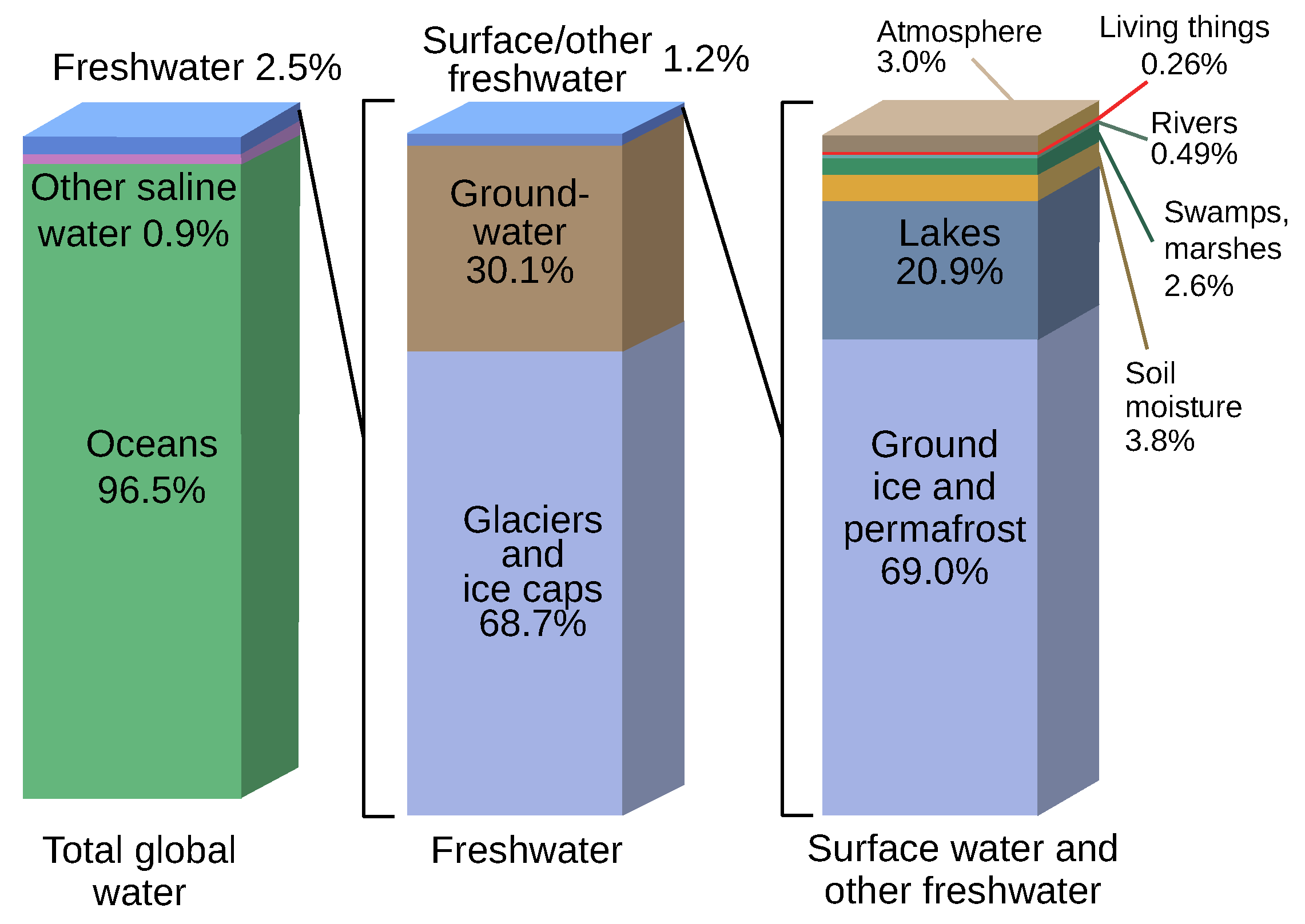
Figure 2.
Review of 3D Reconstruction Methods in Underwater Environments.
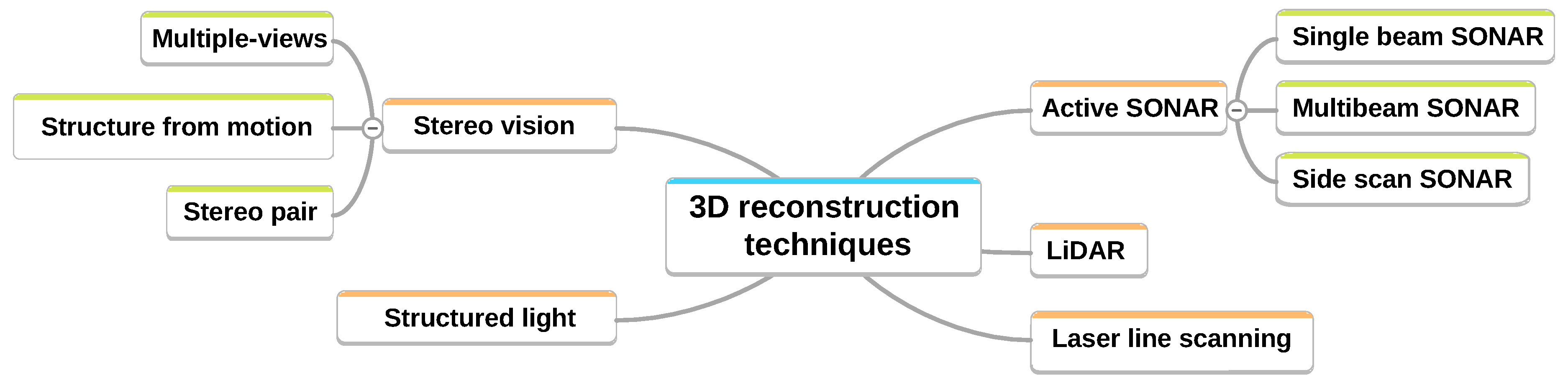
Figure 3.
Flowchart of the camera + projector method.
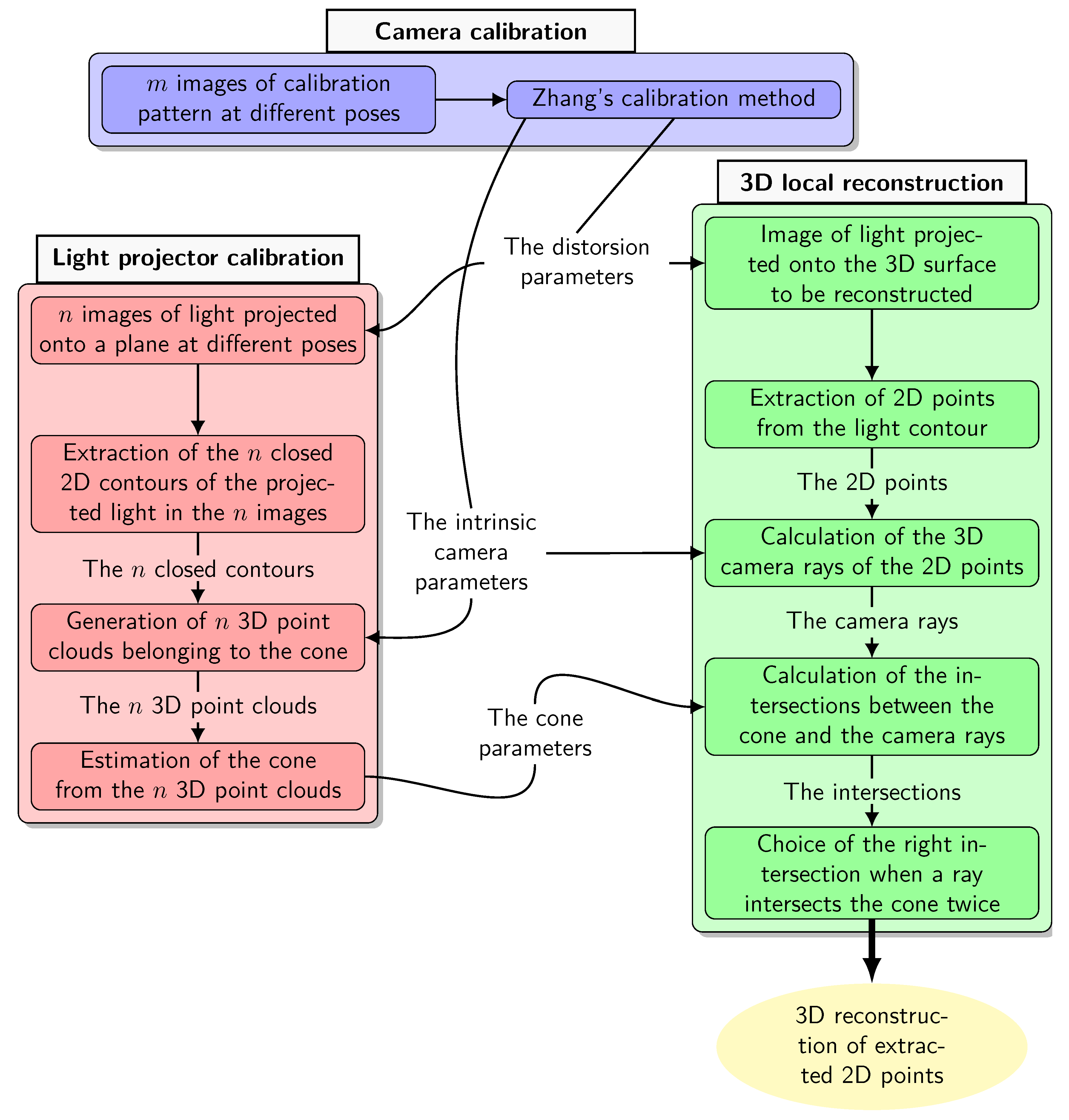
Figure 4.
Diagram of the system consisting of the light projector represented by a cone of revolution and the camera observing the light projection on a plane.
Figure 4.
Diagram of the system consisting of the light projector represented by a cone of revolution and the camera observing the light projection on a plane.
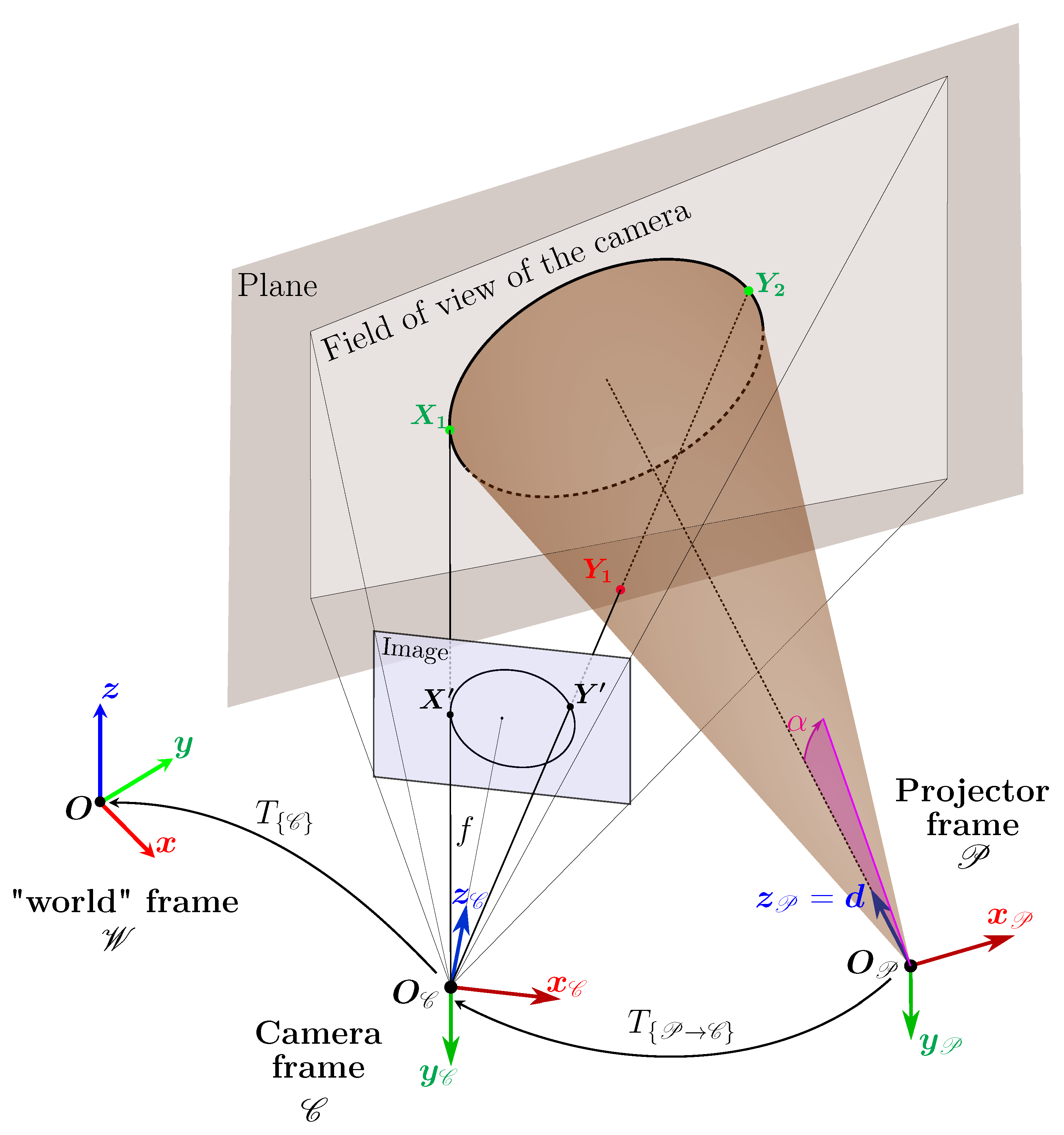
Figure 5.
Parametrisation of the cone using its generatrices. With this parametrisation, we can find the closest generatrix to an external point and thus find the orthogonal projection of this point on the cone.
Figure 5.
Parametrisation of the cone using its generatrices. With this parametrisation, we can find the closest generatrix to an external point and thus find the orthogonal projection of this point on the cone.
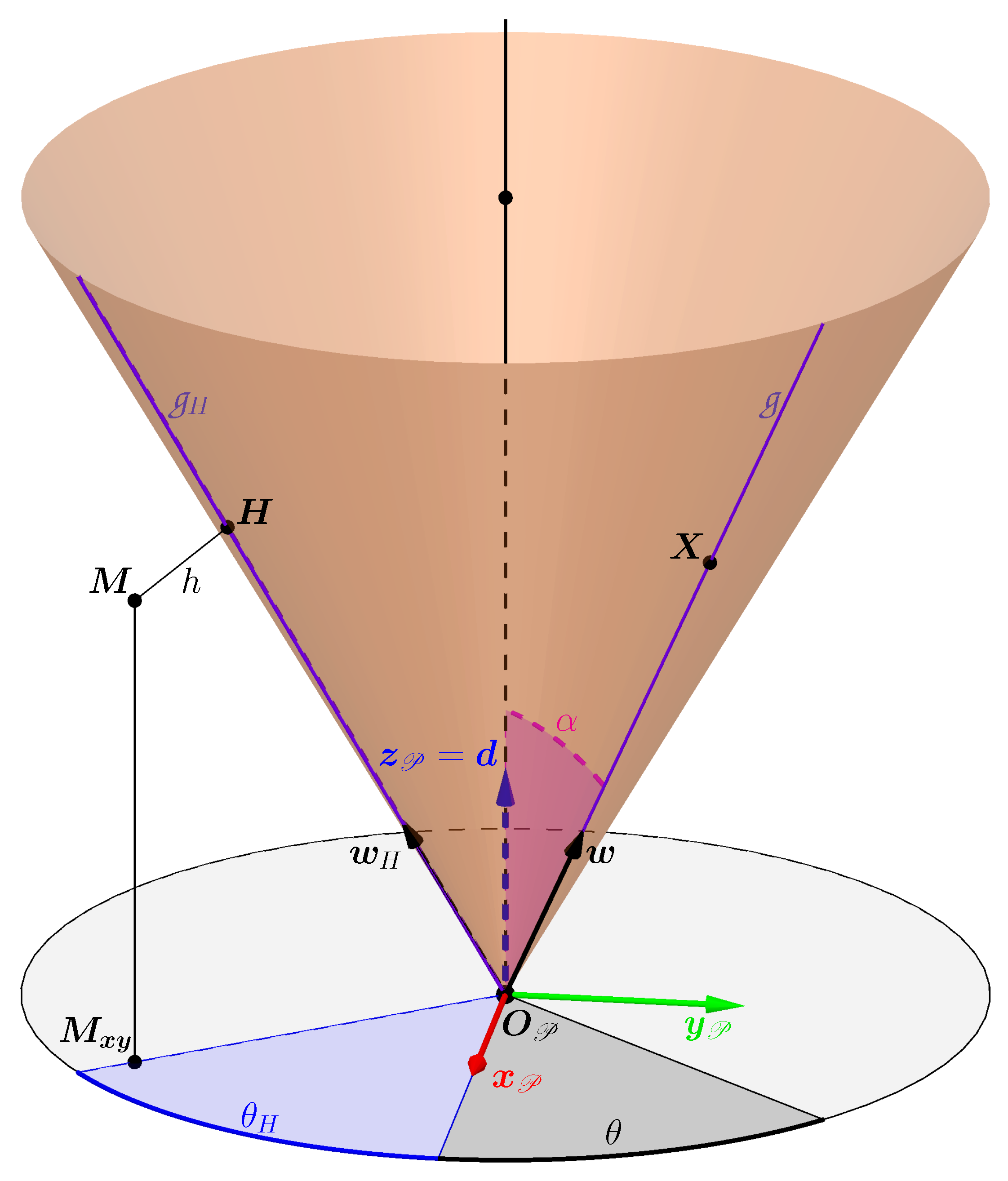
Figure 6.
Example showing the closest points on the upper part of the cone (in red) to points outside the surface of the cone (in blue).
Figure 6.
Example showing the closest points on the upper part of the cone (in red) to points outside the surface of the cone (in blue).
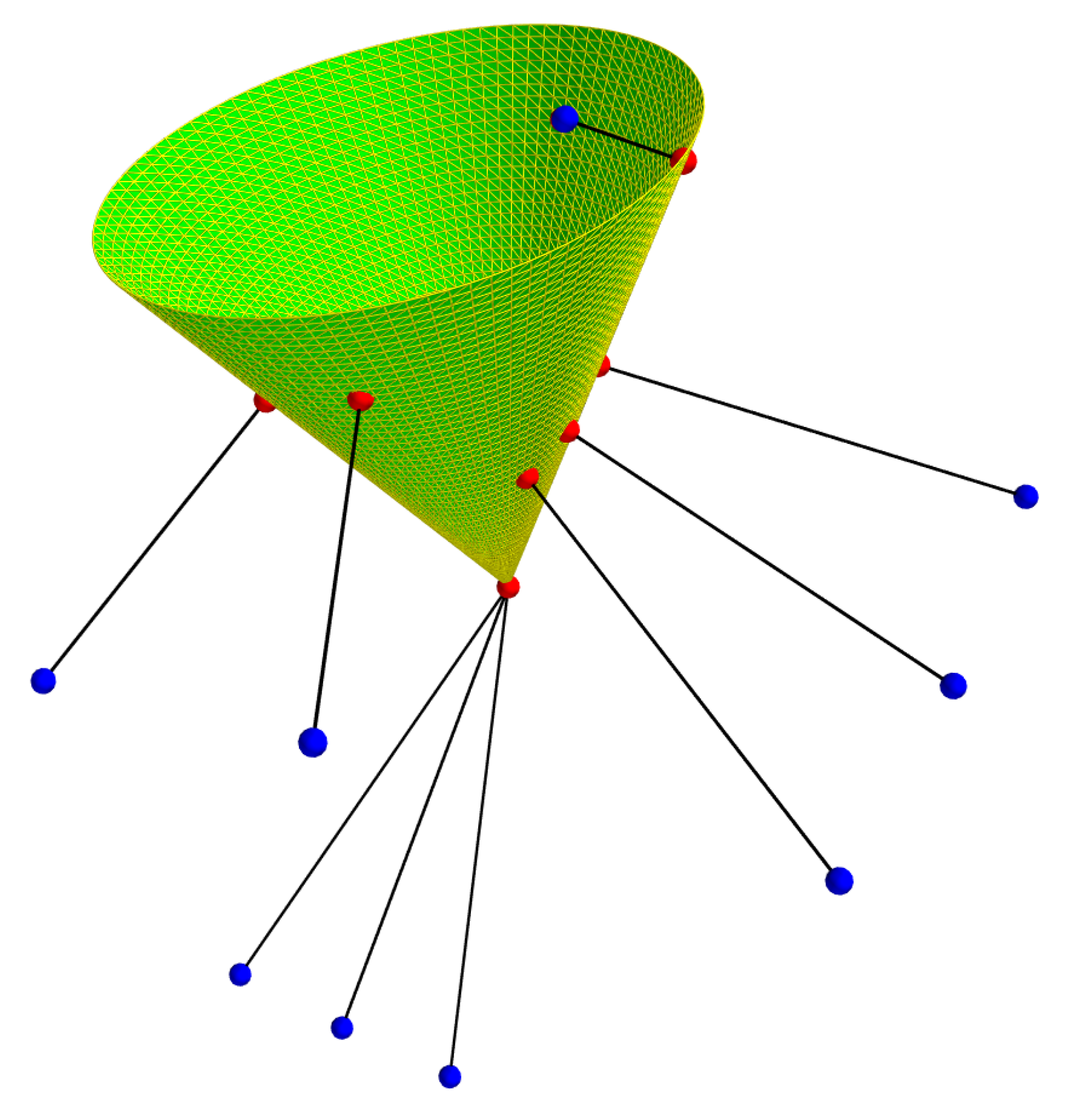
Figure 8.
Method for obtaining several elliptical sections of the cone.
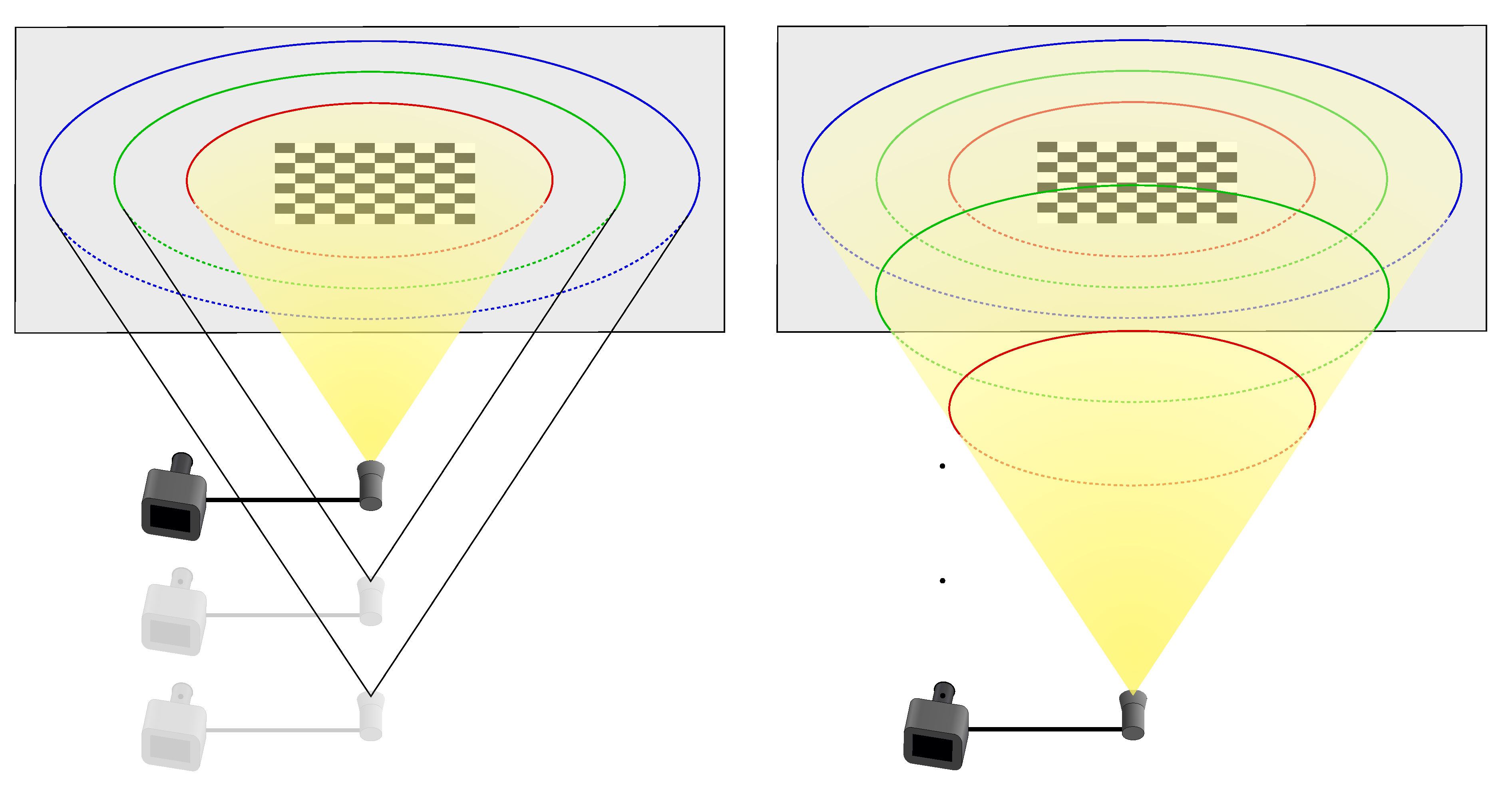
Figure 9.
Representation of the camera / cone pair in an orthogonal projection 2D view where the projection axis is perpendicular to and . The relative orientation of the cone with the camera can be defined here by a single angle called . This is only true if we consider that the camera has an infinite field of view and is therefore symmetrical about its axis defined by (the cone is basically symmetrical about its axis defined by ).
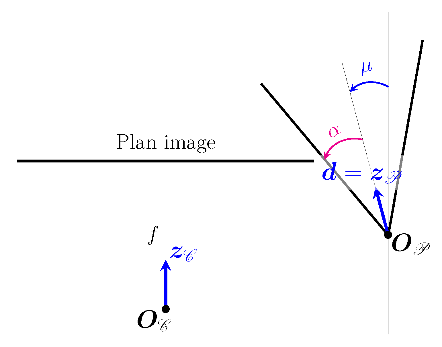
Figure 10.
Representation of the plane when it is not tangent to the cone passing through the optical centre and the two generatrices and .
Figure 10.
Representation of the plane when it is not tangent to the cone passing through the optical centre and the two generatrices and .
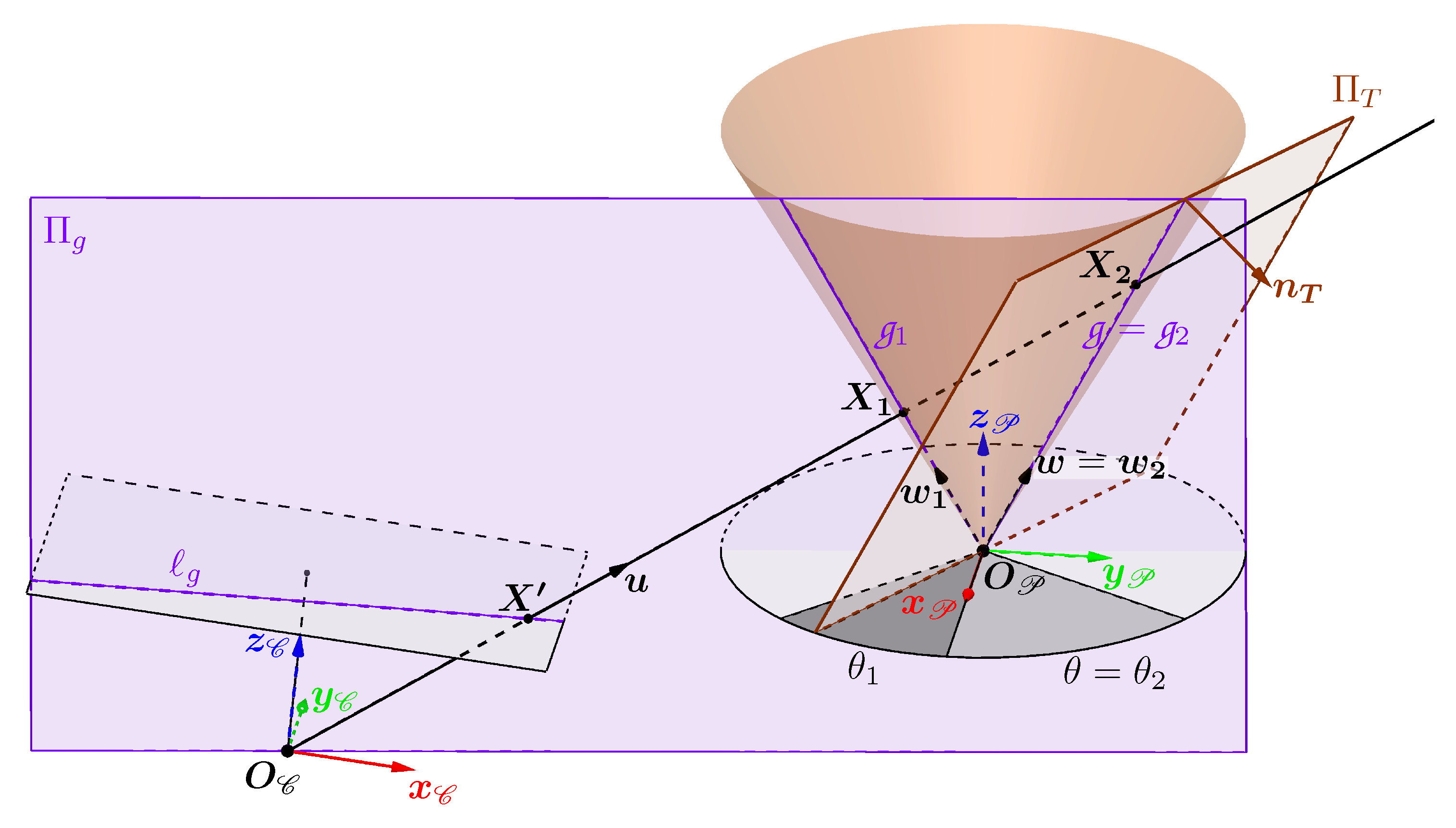
Figure 11.
Representation of fig:conecamtgpl1 and fig:conecamtgpl2, the only two planes tangent to the cone passing through the optical centre.
Figure 11.
Representation of fig:conecamtgpl1 and fig:conecamtgpl2, the only two planes tangent to the cone passing through the optical centre.
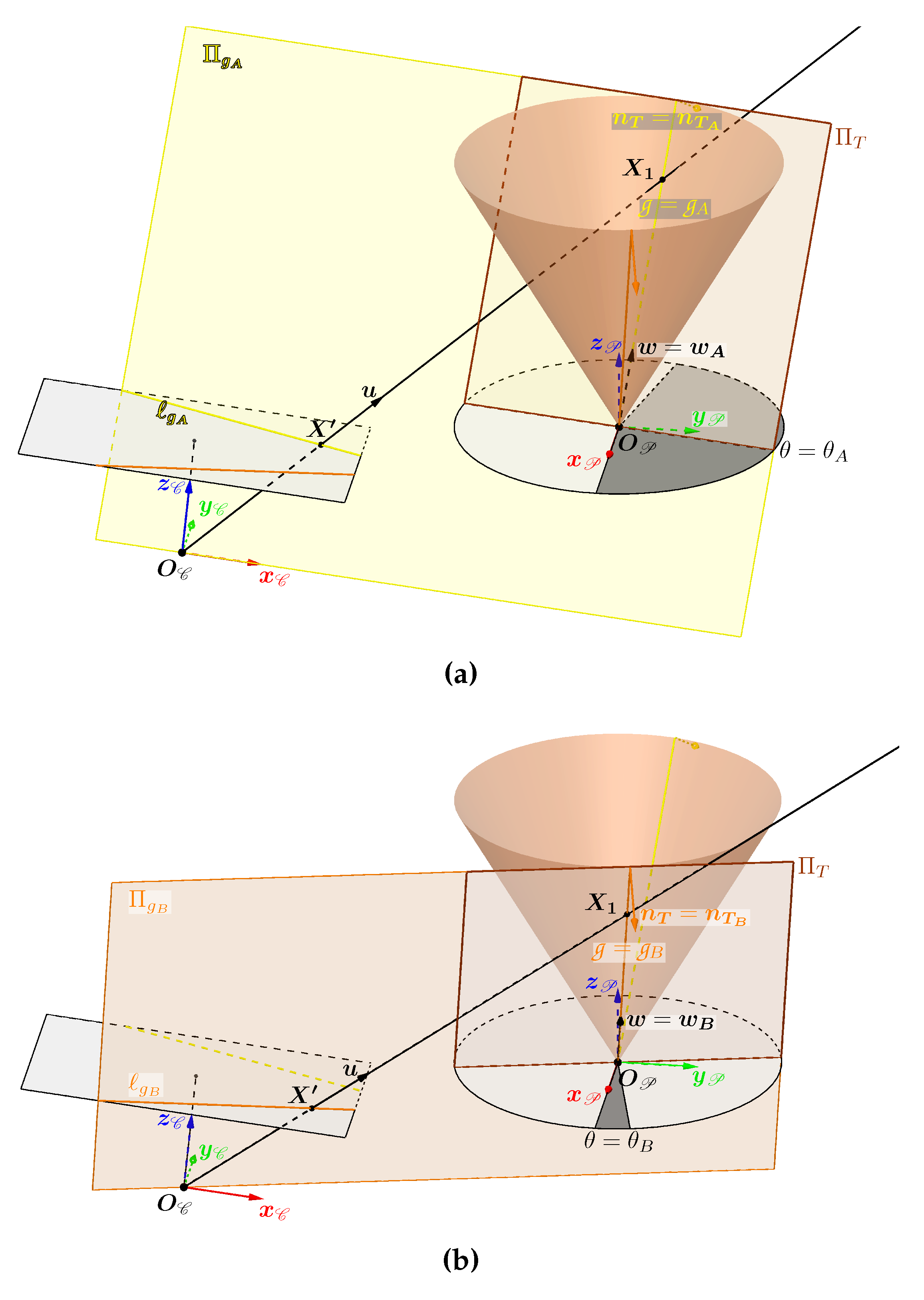
Figure 12.
Visualisation of the vectors and and their angles.
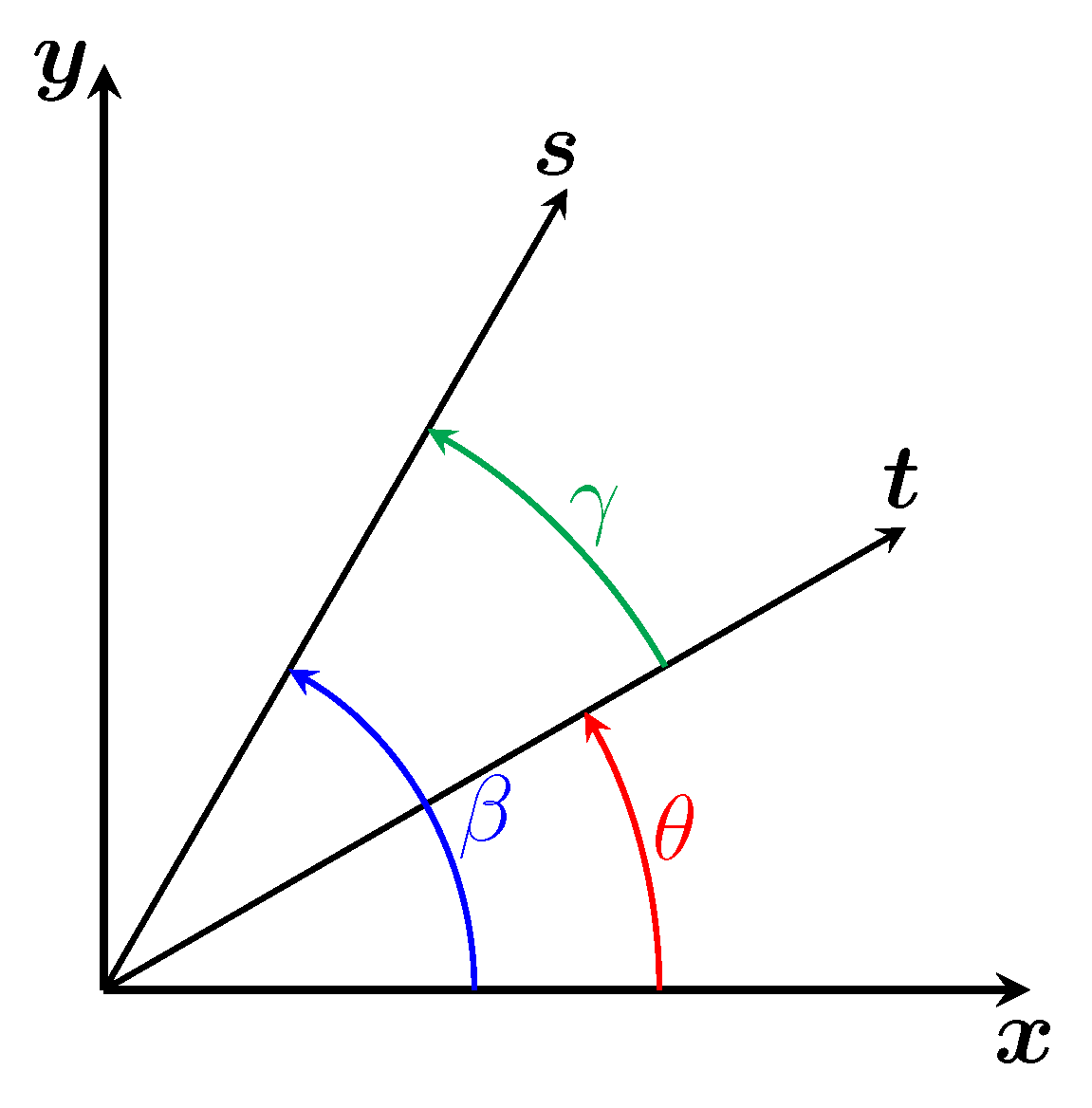
Figure 13.
Representation in the image plane and in the cone of the areas containing the first intersections (in cyan) and the second intersections (in magenta).
Figure 13.
Representation in the image plane and in the cone of the areas containing the first intersections (in cyan) and the second intersections (in magenta).
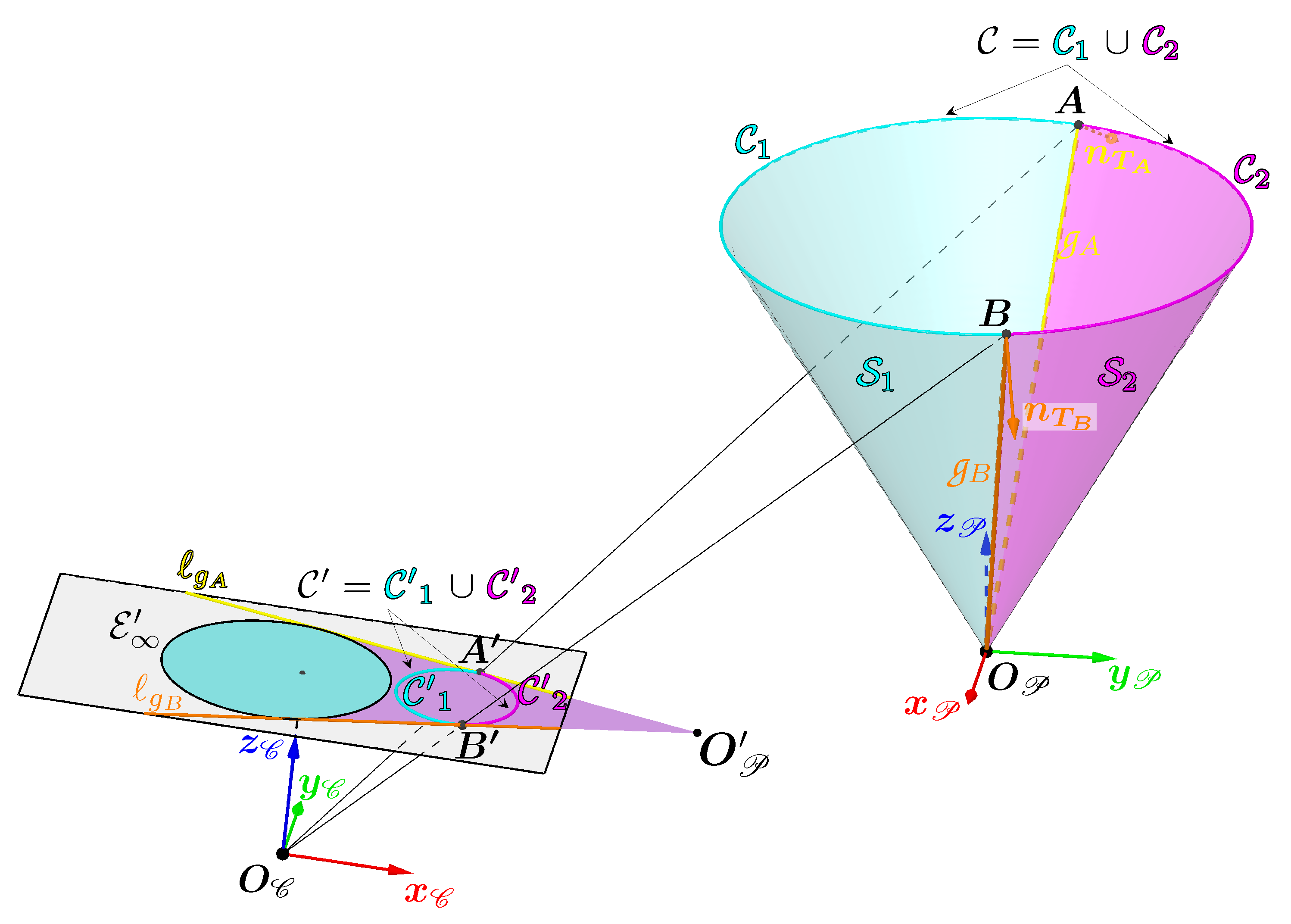
Figure 14.
Representation in the image plane and in the cone of the areas containing the first intersections (in cyan) and the second intersections (in magenta) in the case where part of the cone (in brown) is behind the camera.
Figure 14.
Representation in the image plane and in the cone of the areas containing the first intersections (in cyan) and the second intersections (in magenta) in the case where part of the cone (in brown) is behind the camera.

Figure 15.
Illustrates how to obtain , our reference point in the image plane which indicates the relative position of the cone and which is used to obtain the curves and .
Figure 15.
Illustrates how to obtain , our reference point in the image plane which indicates the relative position of the cone and which is used to obtain the curves and .
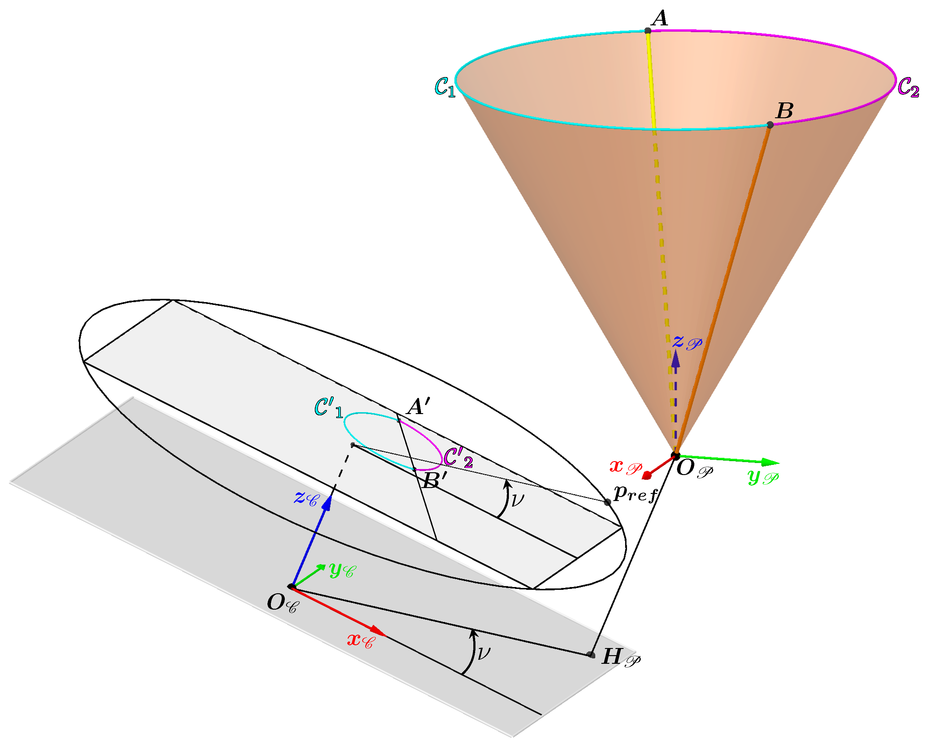
Figure 16.
The camera (represented by a pyramid) and the projector (represented by a cone) arranged inside the model of our gallery to simulate a contour of light in an image. This contour is obtained by projecting the intersections between the generatrices of the cone and the model into the image.
Figure 16.
The camera (represented by a pyramid) and the projector (represented by a cone) arranged inside the model of our gallery to simulate a contour of light in an image. This contour is obtained by projecting the intersections between the generatrices of the cone and the model into the image.
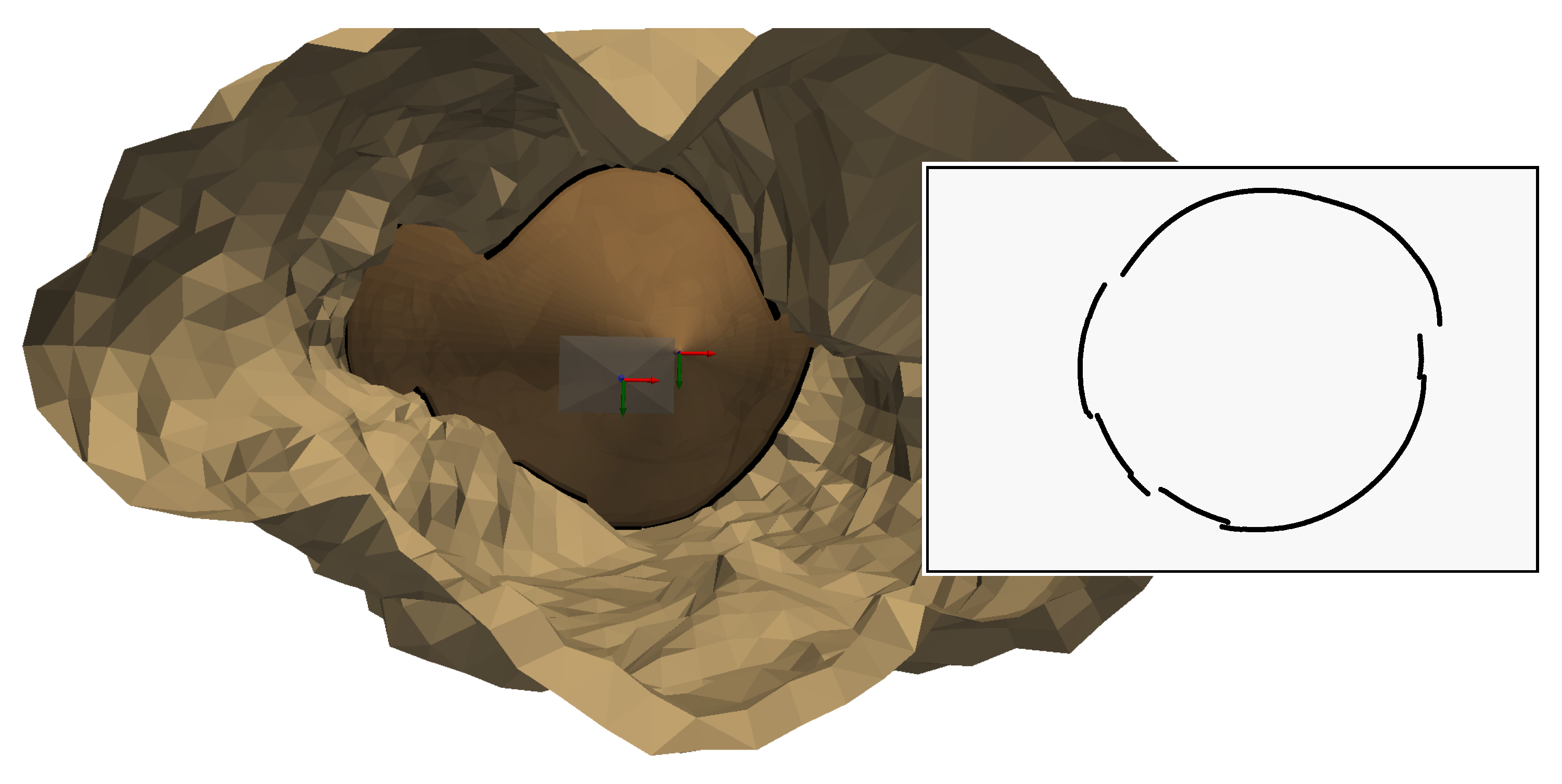
Figure 17.
Determining the points and for our previous example contour.
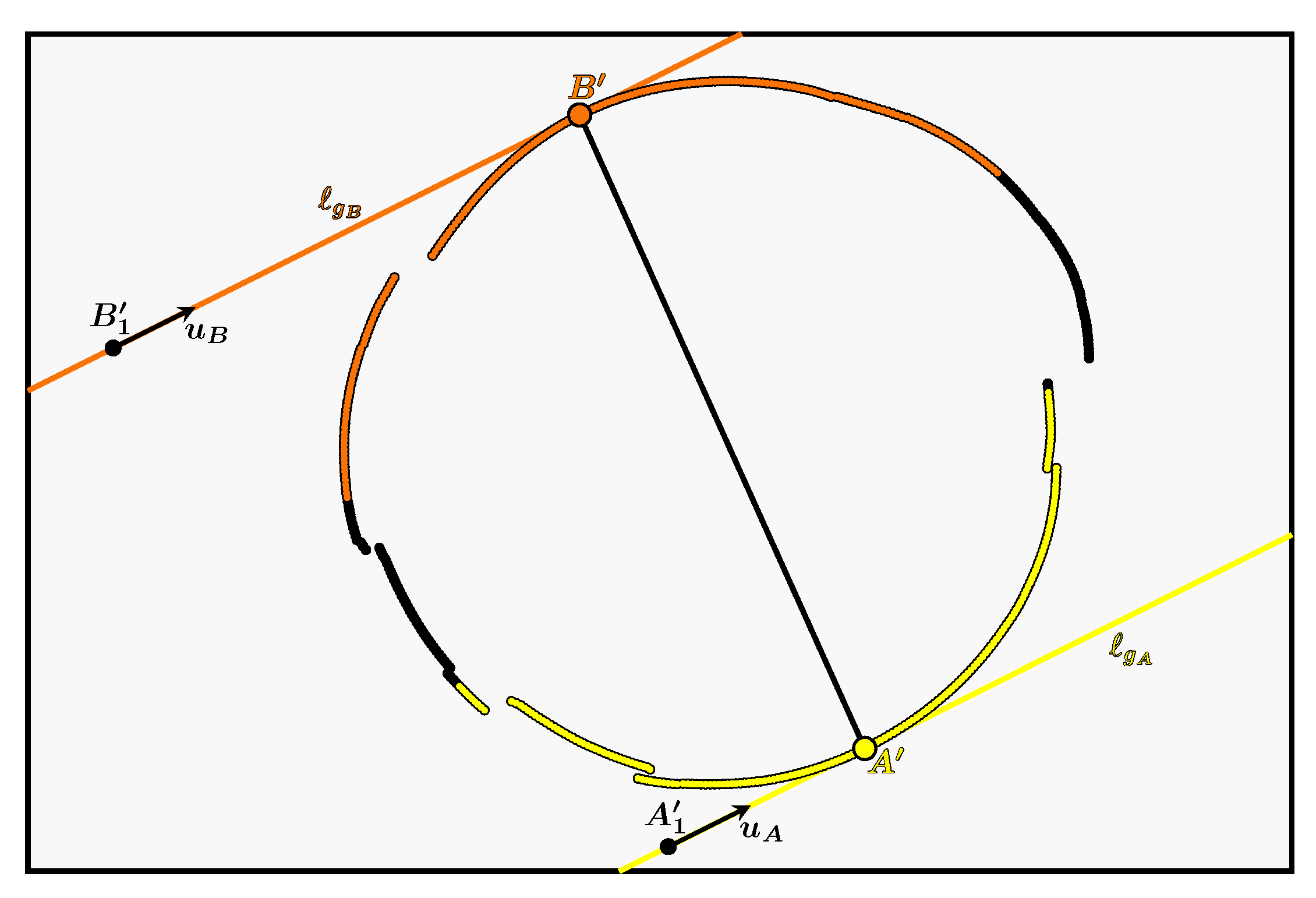
Figure 18.
Determining the curves and for our previous example contour.
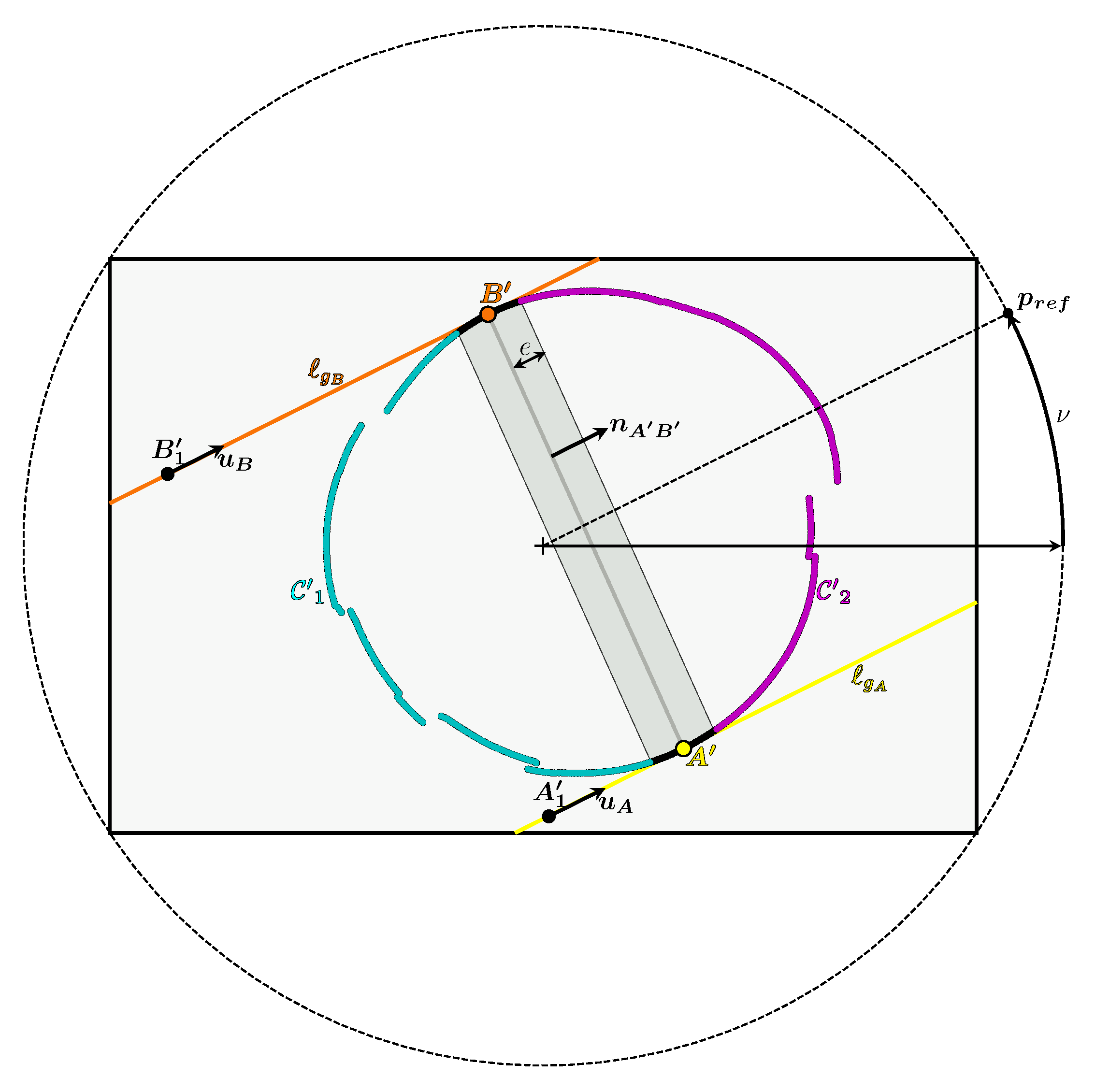
Figure 19.
The reconstructed 3D points added to the 3D scene of Figure 19 with the first intersections in cyan and the second intersections in magenta.
Figure 19.
The reconstructed 3D points added to the 3D scene of Figure 19 with the first intersections in cyan and the second intersections in magenta.
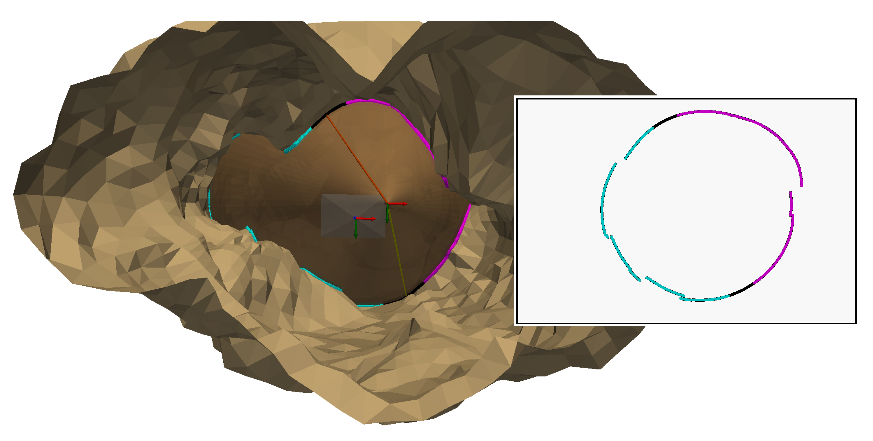
Figure 20.
The diving lamp and its angle of aperture.
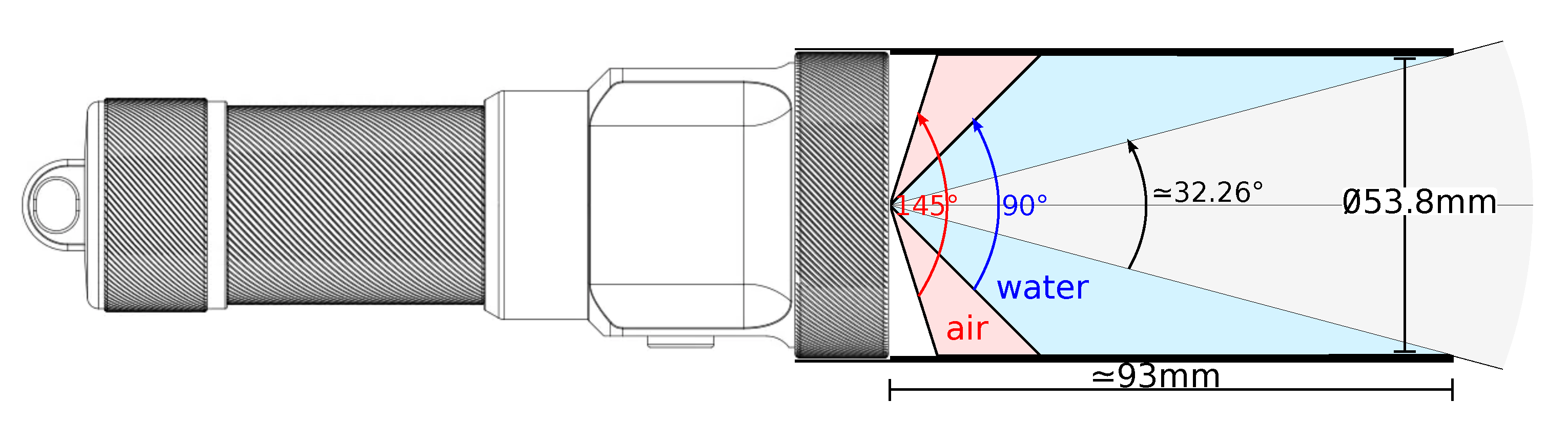
Figure 21.
The system used, consisting of a camera and a conical-shaped projector to which a black cylinder has been added.
Figure 21.
The system used, consisting of a camera and a conical-shaped projector to which a black cylinder has been added.
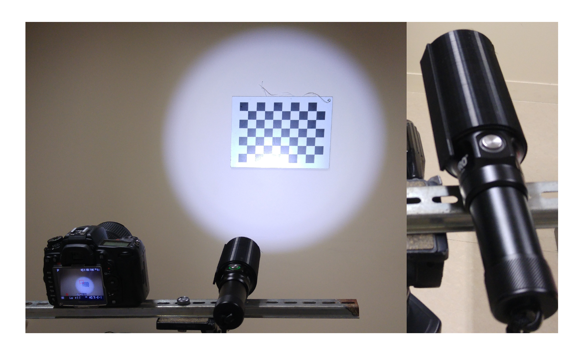
Figure 22.
Image of one of the eight chessboard patterns taken at different poses for camera calibration using Zhang’s method.
Figure 22.
Image of one of the eight chessboard patterns taken at different poses for camera calibration using Zhang’s method.
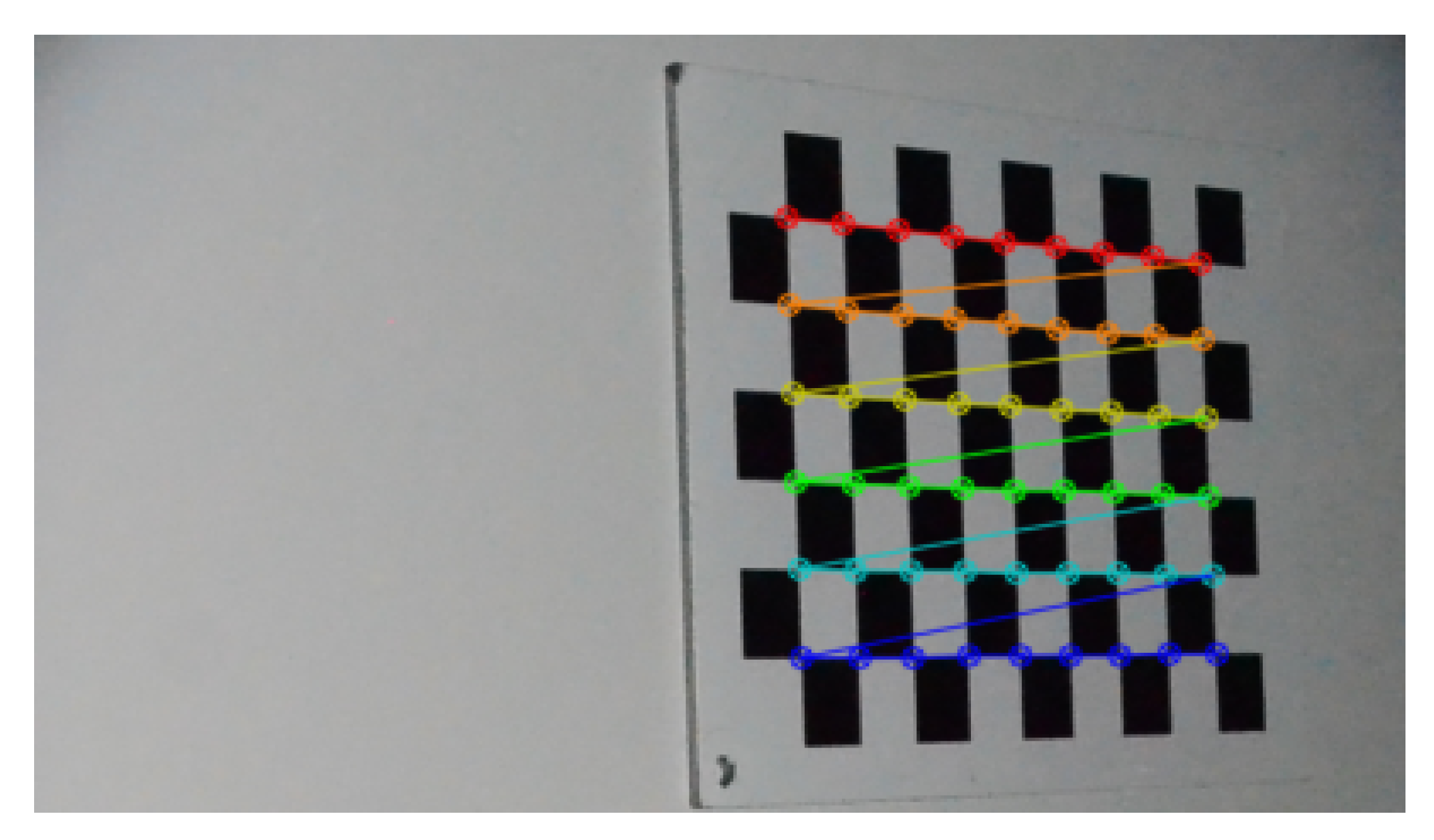
Figure 23.
3D view of the chessboard in its eight poses in relation to the camera.
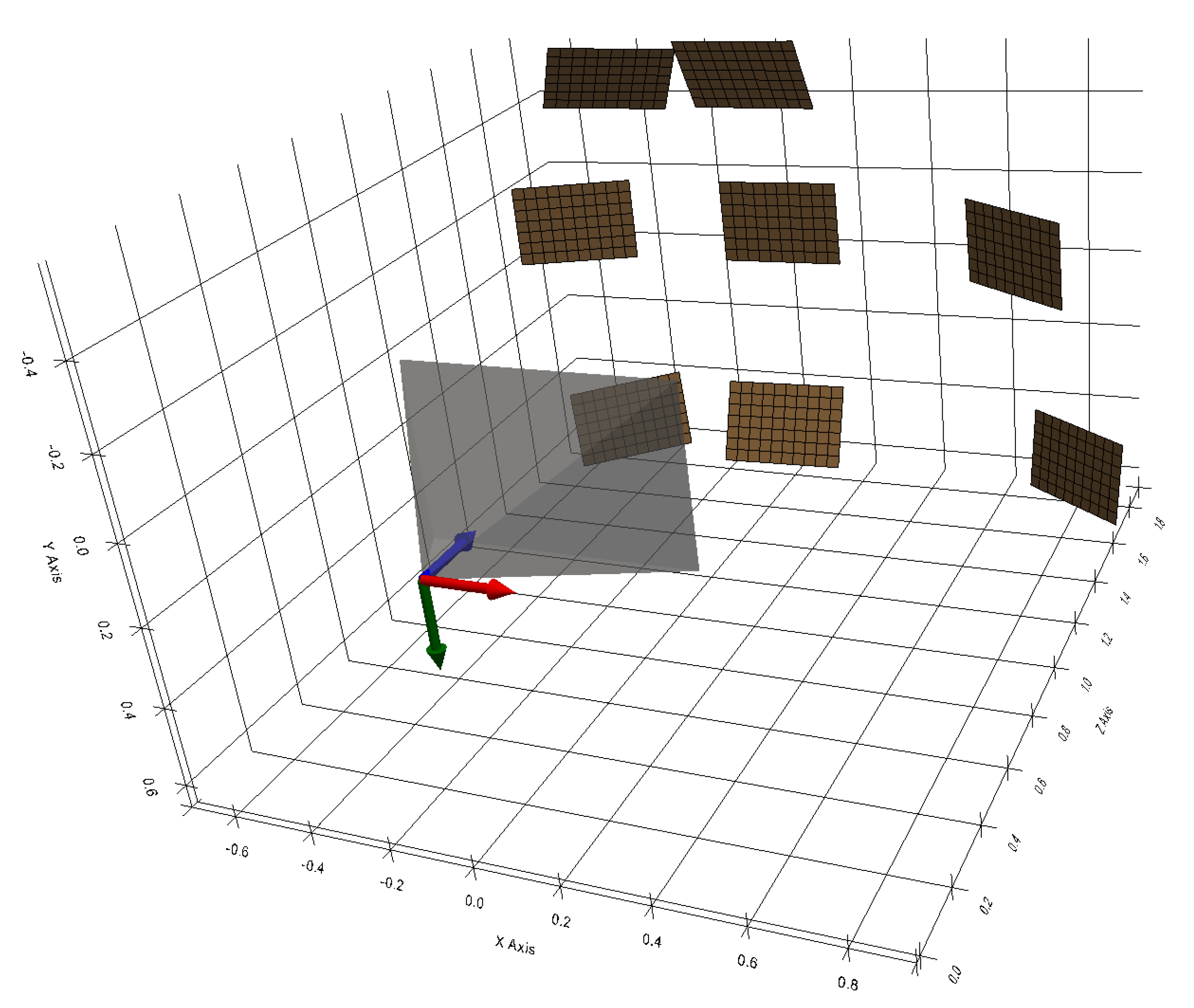
Figure 24.
2 images of light projected onto the wall from the five where the axis of the projector is almost orthogonal to the wall (images 1 and 5).
Figure 24.
2 images of light projected onto the wall from the five where the axis of the projector is almost orthogonal to the wall (images 1 and 5).
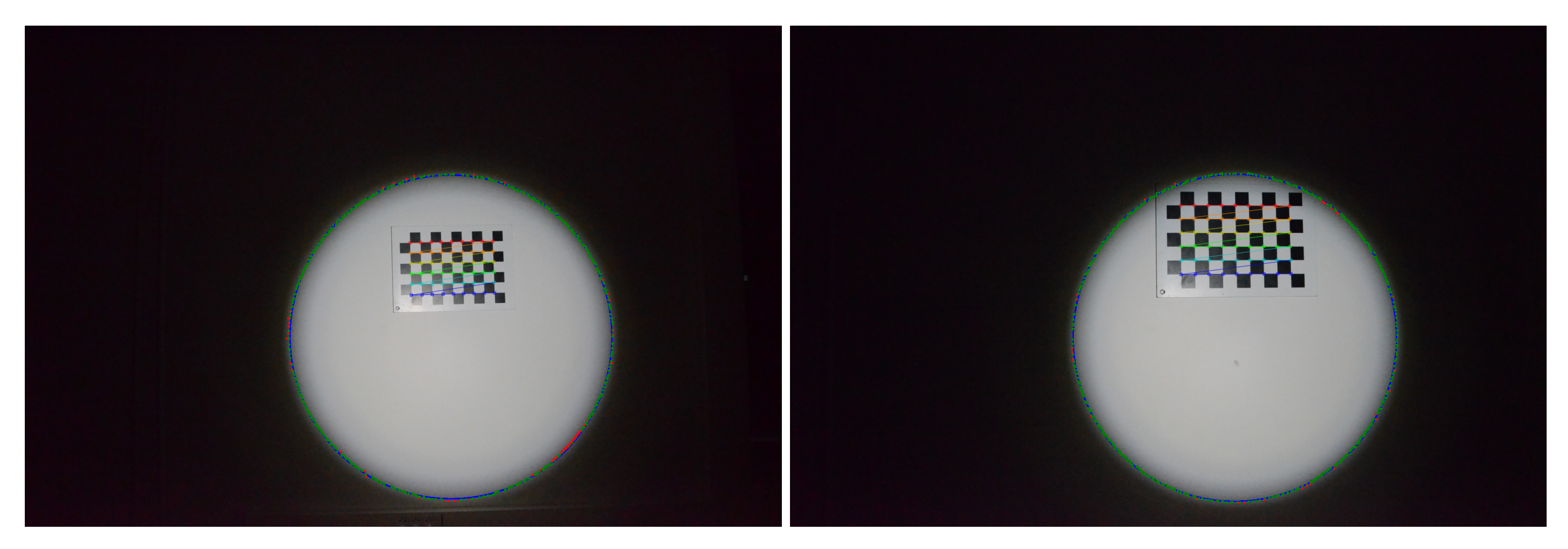
Figure 25.
3D view of the elliptical sections, the camera and the chessboard pattern. In the image on the left, the elements are expressed in the pattern frame. In the image on the right, the elements are expressed in the camera frame.
Figure 25.
3D view of the elliptical sections, the camera and the chessboard pattern. In the image on the left, the elements are expressed in the pattern frame. In the image on the right, the elements are expressed in the camera frame.
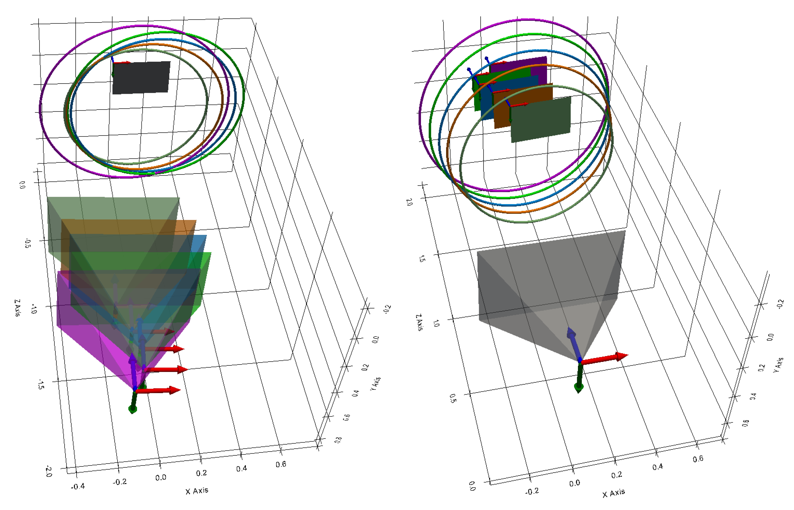
Figure 26.
Representation of the estimated cone in relation to elliptical sections where the colour of the points depends on the distance orthogonal to the cone.
Figure 26.
Representation of the estimated cone in relation to elliptical sections where the colour of the points depends on the distance orthogonal to the cone.
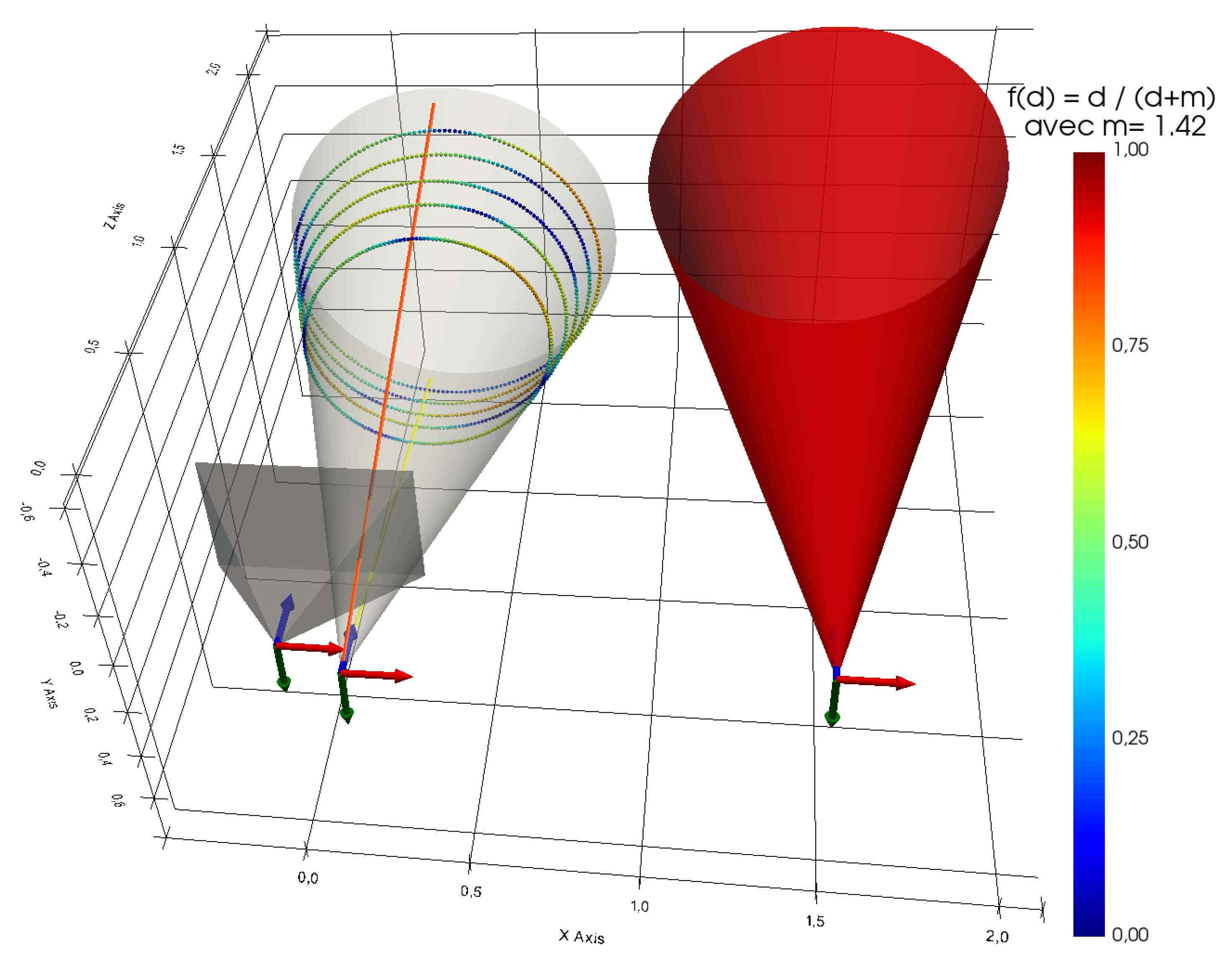
Figure 27.
2 images in the aqueduct with light contours.
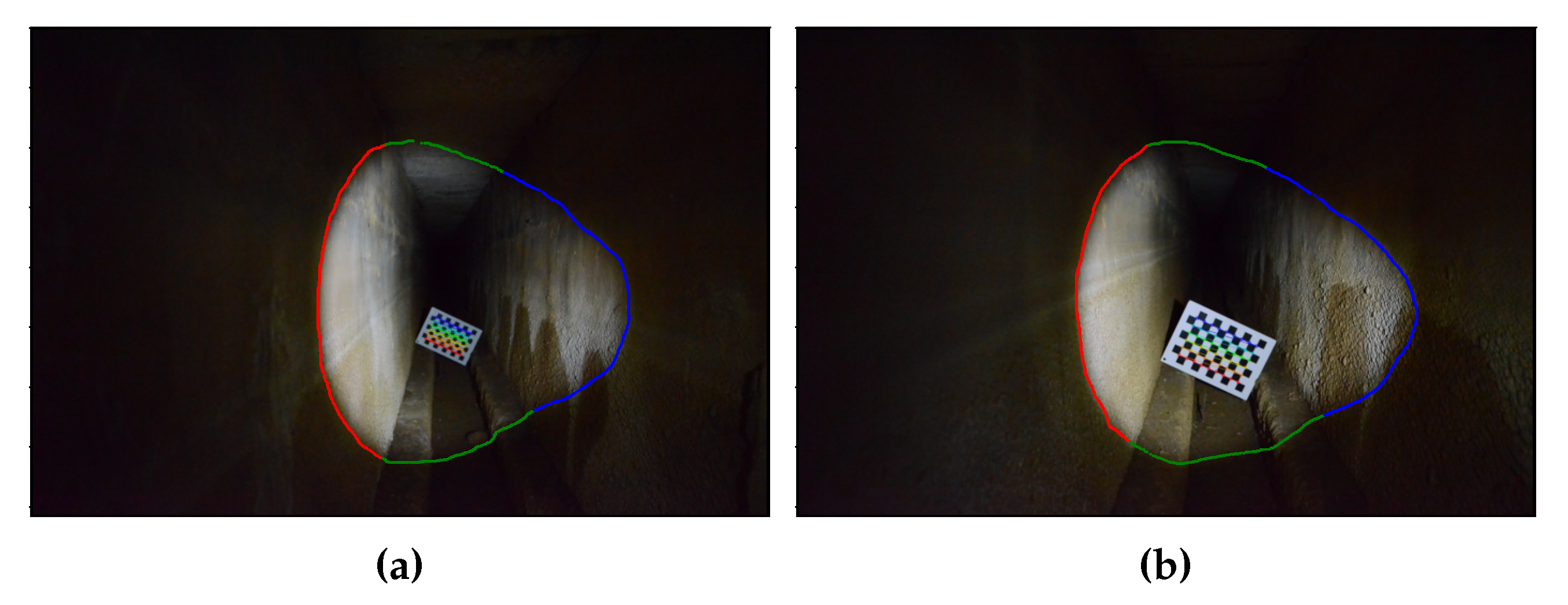
Figure 28.
Intersection selection.
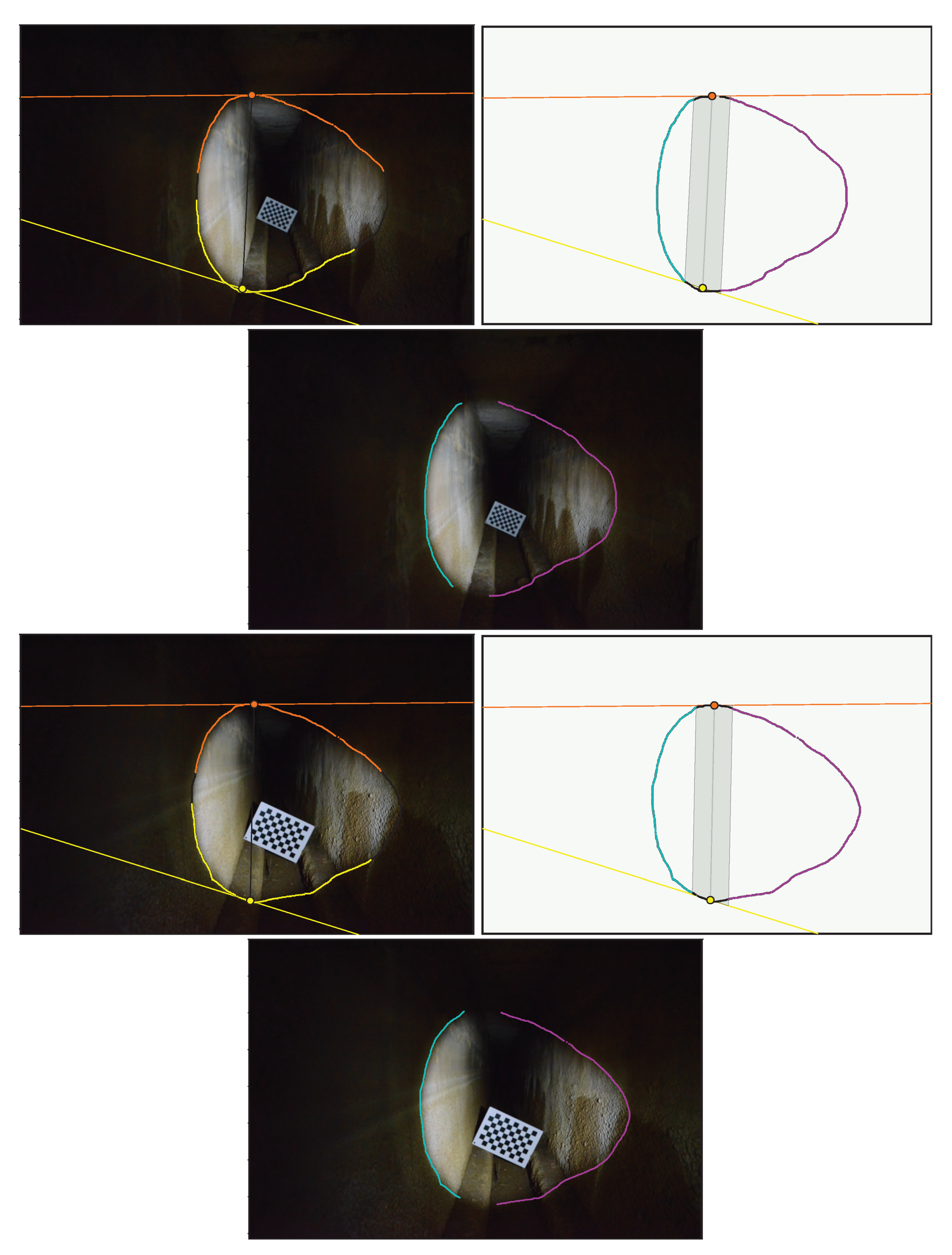
Figure 29.
3D reconstruction of the contours extracted from the six images.
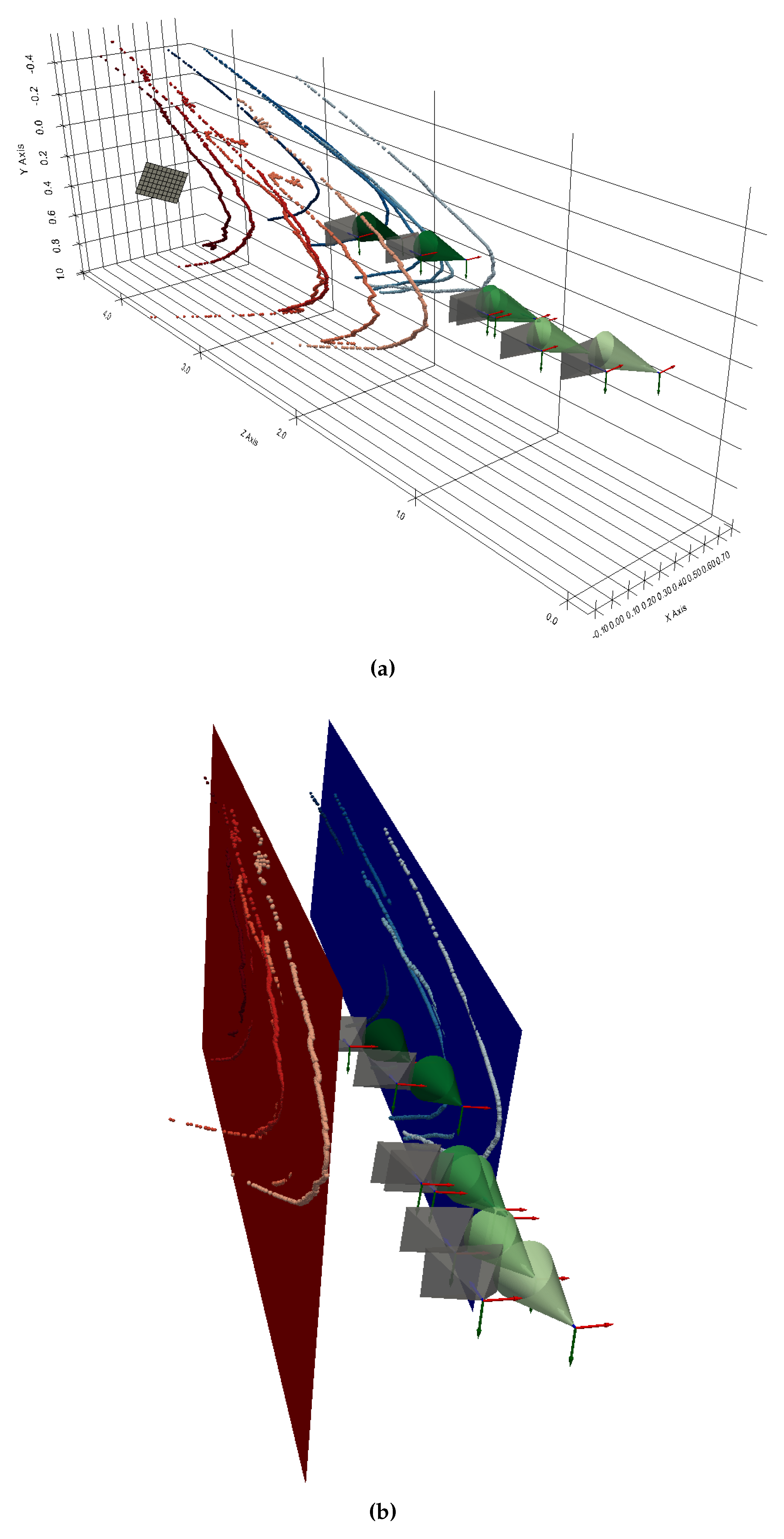
Figure 30.
Configuration with 4 cameras.
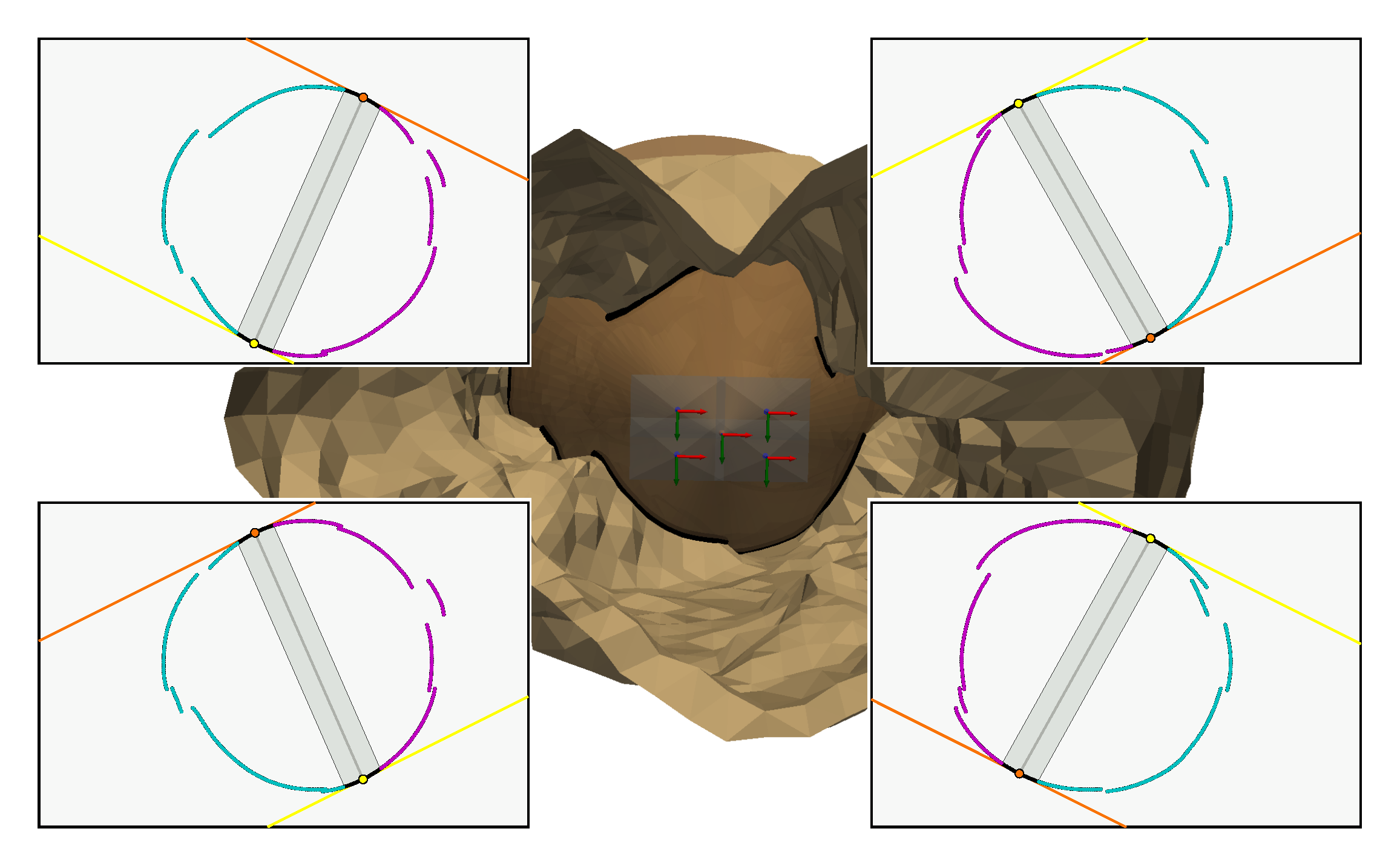

Table 1.
Comparison of estimated and measured cone parameters.
| Estimated values | Measured values | Relative deviation | |
|---|---|---|---|
| from measurement | |||
| 14,79° | 16,13° | 1,34° (-8%) | |
| 0,210m | 0,212m | -0,002m (-0.9%) |
Table 2.
Statistics of the orthogonal distances in mm between the 3D points of each elliptical section and the estimated cone.
Table 2.
Statistics of the orthogonal distances in mm between the 3D points of each elliptical section and the estimated cone.
| Dist. (mm) | Max. | Min. | Med. | Moy. | RMS |
|---|---|---|---|---|---|
| Section 0 | 4,2 | 0,0 | 1,4 | 1,5 | 2,0 |
| Section 1 | 3,3 | 0,0 | 1,5 | 1,5 | 1,8 |
| Section 2 | 4,1 | 0,0 | 1,4 | 1,6 | 2,0 |
| Section 3 | 3,4 | 0,0 | 1,6 | 1,6 | 1,8 |
| Section 4 | 3,6 | 0,0 | 1,3 | 1,5 | 1,8 |
| All | 4,2 | 0,0 | 1,4 | 1,5 | 1,9 |
Table 3.
Distance statistics in mm between the 3D points of each elliptical section and the reconstructed 3D points.
Table 3.
Distance statistics in mm between the 3D points of each elliptical section and the reconstructed 3D points.
| Dist. (mm) | Max. | Min. | Med. | Moy. | RMS |
|---|---|---|---|---|---|
| Section 0 | 94,0 | 0,4 | 28,5 | 27,7 | 32,6 |
| Section 1 | 149,6 | 0,0 | 23,6 | 30,9 | 42,8 |
| Section 2 | 226,1 | 0,1 | 18,6 | 33,6 | 51,3 |
| Section 3 | 179,3 | 0,1 | 18,6 | 30,0 | 44,7 |
| Section 4 | 114,3 | 0,1 | 19,8 | 23,0 | 29,1 |
| All | 226,1 | 0,0 | 20,6 | 29,0 | 40,9 |
Table 4.
Orthogonal distances between 3D points and estimated planes.
| Dist. (mm) | Max. | Min. | Med. | Moy. | RMS |
|---|---|---|---|---|---|
| Left 3D points | 220.5 | 0.0 | 11.0 | 13.9 | 19.9 |
| to left plane | |||||
| Right 3D points | 113.9 | 0.0 | 20.4 | 24.1 | 30.5 |
| to right plane | |||||
| Left 3D points | 778.4 | 492.1 | 581.9 | 584.9 | 585.2 |
| to right plane | |||||
| Right 3D points | 691.1 | 476.9 | 585.2 | 583.6 | 584.4 |
| to left plane |
Disclaimer/Publisher’s Note: The statements, opinions and data contained in all publications are solely those of the individual author(s) and contributor(s) and not of MDPI and/or the editor(s). MDPI and/or the editor(s) disclaim responsibility for any injury to people or property resulting from any ideas, methods, instructions or products referred to in the content. |
© 2024 by the authors. Licensee MDPI, Basel, Switzerland. This article is an open access article distributed under the terms and conditions of the Creative Commons Attribution (CC BY) license (http://creativecommons.org/licenses/by/4.0/).
Copyright: This open access article is published under a Creative Commons CC BY 4.0 license, which permit the free download, distribution, and reuse, provided that the author and preprint are cited in any reuse.


