Submitted:
28 April 2024
Posted:
29 April 2024
You are already at the latest version
Abstract
This paper proposes a novel concept within Quantum Natural Language Processing (QNLP) to encode the interpersonal metafunction of Systemic Functional Linguistics (SFL), particularly tenor, into quantum circuits by treating Japanese honorifics seriously. Because of English language bias in the literature, the incorporation of nuanced aspects of interpersonal communication evident in languages, such as the aforesaid Japanese, remains under-developed and overlooked. Utilizing lambeq, monoidal categories, and string diagrams, this study extends lambeq’s quantum computing framework to capture not only grammar but also social context—specifically the roles and relationships that define interpersonal interactions in quantum circuits. This approach represents a significant step toward that end simply by defining the honorific type h in lambeq. This innovative strategy exposes the capability of quantum circuits to model the complex structures of language, moving beyond grammar and even semantics—the horizontal, textual dimension of language—to embrace the vertical, hierarchical dimension of human communication and social interaction. Through this lens, the paper underscores the potential of QNLP to transcend traditional linguistic analysis, advocating for a broader and more nuanced understanding of language that includes not only what is said but also the social persona of the interlocutors. An algorithm for parsing Japanese grammar into pregroup diagrams containing the h type is introduced along with a codebase for other researchers to use and to which to contribute. Lastly, a toy experiment is performed to demonstrate that the circuits generated from these pregroup diagrams are suitable for Quantum Machine Learning (QML) applications.
Keywords:
Quantum Natural Language Processing
; QNLP
; Systemic Functional Linguistics
; SFL
; Japanese
; honorifics
; interpersonal metafunction
; lambeq
; category theory
; Quantum Machine Learning
; QML
1. Introduction: Hiding in Plain Sight
Language is the manifestation of human cognition and social interaction, encoding not only the exchange of information but also a complex web of ideas, experiences, social relationships, emotions, and cultural norms. It is indeed the framework of reality itself (Coecke, 2016; Walton, 2024a). Systemic Functional Linguistics (SFL) is a theory positing that language operates on multiple levels, including the experiential, the logical, and the interpersonal (Matthiessen & Halliday, 1997). The interpersonal metafunction underscores how language acts as a tool for speakers to negotiate social roles and relationships—a dimension of language that is richly encoded in the honorific systems of languages like Japanese (Sekizawa & Yanaka, 2023).
The core of this paper is an endeavor to see the encoding of the interpersonal metafunction of SFL into quantum circuits, using the nuanced system of Japanese honorifics as the object of the study. This initiative is motivated by a recognition of the significant English language bias in current Natural Language Processing (NLP) and Quantum Natural Language Processing (QNLP) literature, a bias that inadvertently obfuscates the rich interpersonal nuances that are hiding in plain sight from the perspective of high-context languages like Japanese (Hall, 1976). This study leverages the formidable capabilities of lambeq to create monoidal categories and string diagrams to demonstrate the encoding of the interpersonal metafunction into a quantum circuit (Kartsaklis et al., 2021; Quantinuum, 2024b). Though using lambeq presents challenges when working with Japanese, it is an excellent toolkit with great potential for growth and utilization in academic research. Indeed, the adaptation of lambeq to accommodate the complexities of Japanese honorifics is no small task. The transition from the depCCG parser to the English-centric, though more efficient, BobcatParser underscores the pressing need to confront and mitigate the prevailing English language bias (Yoshikawa, 2023a; Quantinuum, 2024a). While it is technically possible to deploy the depCCG parser with lambeq’s 0.4.0 release, there is no formal support for doing so, and the depCCG parser itself has a bug that makes installation and use a roadblock for most (Quantinuum 2024c; Yoshikawa, 2023b). The lack of formal support for depCCG, then, will potentially make the effort required for its use in the future prohibitive. This is, ultimately, an opportunity for the BobcatParser to incorporate support for various foreign languages and afford the broader community of researchers with the opportunity to share insights from their native tongues with the world.
Nevertheless, this paper proposes a novel interpretation, a first step toward a richer implementation of the interpersonal metafunction in a quantum circuit, without needing to extend lambeq with Japanese language support, though that is needed and an avenue for further research. The tool in its present state allows the definition of arbitrary grammar types. This, then, affords the opportunity to define an honorific type h, which encapsulates a core element, known by the same name, of interpersonal relationships and social roles as manifested in the Japanese language.
This endeavor, then, is not merely a technical exercise that offers a new starting point for working with Japanese in lambeq in the form of executable software. It is also a philosophical exploration that seeks to bridge the horizontal dimension of language—its grammar and semantics—with the vertical, hierarchical dimension of interpersonal relationships, social interactions, and meaning itself. In doing so, this paper positions itself at the intersection of quantum computing, linguistics, social theory, ethics, and philosophy proposing that QNLP can and should encompass the full spectrum of language's multifunctionality.
1.1. Purpose
In essence, this paper is an invitation to reimagine the possibilities of QNLP, urging the field to embrace the complexity and richness of language in its entirety. Through an introductory-level and technical examination of Japanese honorifics within a quantum computational framework, this study endeavors to illuminate the path toward a more inclusive, nuanced, and profound understanding of language, one that acknowledges and celebrates the interpersonal as much as the textual and informational.
1.2. Contributions and Their Avenues for Further Research
QNLP, a nascent yet potentially potent domain, aims to leverage the peculiarities of quantum mechanics to unravel the intricate tapestry of human language. In other words, it encodes grammatical and semantic relationships between words or sentences depending on the level of granularity (Coecke, 2020; Wang-Máscianica, Liu, & Coecke, 2023). This is made possible by the shared mathematical structure of language and quantum mechanics (Coecke et al., 2020; Coecke et al., 2021). This paper, then, provides several novel contributions to further the field and opens the path to further research focused on each contribution as well:
- It proposes using lambeq’s type functionality to encode honorifics as a type separate from nouns or noun-phrases. This invites further research into other potential types, as proposed previously, and research into the more intricate features of Japanese honorifics and particles as theorized in Walton, 2023. Additionally, a toy experiment using the h type is performed to encourage more robust and meaningful experiments in the future.
- It provides an alternative starting point for other researchers to build their own Japanese experiments without relying on the depCCG parser. The source code is available on GitHub, and others are invited to contribute by extending the grammar model, improving the algorithm, and the like (Walton, 2024b). This starting point could easily be expanded and perhaps built into a lambeq package or incorporated into a robust parser in further research.
- It invites researchers and developers to consider what is being overlooked due to language bias and to attempt to mitigate said bias. Opening the mind to consider other information that may be encoded in quantum circuits is a significant area for further research.
- Lastly, it introduces a simple model based on Japanese honorifics for considering language content across two dimensions: the horizontal and the vertical. Applying more mathematical rigor to this model to present it as a conceptual space and potentially extending it to account for additional metafunctions of SFL are avenues for research here.
2. Background
2.1. A Very Brief Literature Review
This paper situates its contributions within the broader context of ongoing research in QNLP, drawing connections to previous work that has explored the encoding of linguistic structures and meanings within quantum circuits to various ends. There has been a great deal of work on diagrammatic reasoning using DisCoCat, DisCoCirc (or “text circuits”), internal wirings, ZX-calculus, and more (Coecke, 2010; Coecke, 2020; Coecke & Kissinger, 2017; Coecke & Gogioso, 2022; Coecke, Lewis, & Marsden, 2018; Wang-Máscianica et al., 2023; Liu et al., 2023; Rizzo, 2019; Waseem et al., 2022; van de Wetering, 2020). This work leverages algebraic grammar, category theory, and Frobenius algebras as the mathematical basis of the diagrams as well as the underpinning of the larger compositional nature of discourse and of reality itself (Lambek, 1997; Cardinal, 2002; Cardinal, 2007; de Felice, 2022: Coecke & Paquette, 2009; Yeung & Kartsaklis, 2021; Toumi, 2022; Kartsaklis, 2015; Coecke, 2021; Coecke et al., 2018; Coecke, Sadrzadeh, & Clark, 2010). This mathematical basis demonstrates a connection between simulating nature and understanding grammar (Feynman, 1982). Additionally, work has been done to create algorithms, software packages, such as the aforesaid lambeq, that support research and experimentation using these ideas (Zeng & Coecke, 2016; de Felice, Toumi, & Coecke, 2021; Kartsaklis et al, 2021). Several different linguistic phenomena have been studied in detail, such as hyponymy, entailment, logical and conversational negation, worldly context, representing relative pronouns, parsing conjunctions, with more work underway (Rodatz, Shaikh, & Yeh, 2021; Shaikh et al., 2022; Lewis, 2019; Lewis, 2020; de las Cuevas et al., 2020; Coecke & Wang, 2021; Duneau, 2021). Machine learning classification, machine translation, and other intelligence models have also been the subject of on-going research (Meichanetzidis et al., 2023; Abbaszade et al., 2021; Abbaszade et al., 2023; Nieto, 2021; Lorenz et al., 2021; Coecke et al., 2021; García, Cruz-Benito, & García-Peñalvo, 2023). Lastly, there have even been applications of these ideas in the artistic realm of music as well as the realm of computer vision (Putz & Svozil, 2015; Xue et al., 2024). The ideas presented here are indebted to the research cited above. This is by no means a full literature review, but it is enough to initiate the interested and to provide needed context for what follows.
2.2. Two Special Acknowledgements
Of all the wonderful work cited here, two papers deserve thanks for inspiring the insights of this study. First, in “Talking Space: inference from spatial linguistic meanings”, Wang-Maścianica and Coecke demonstrated that DisCoCat diagrams can encode spatial meaning as well as arbitrarily defined conceptual spaces (2021). That idea is the primary inspiration for the proposition that these diagrams can encode more than textual grammar and semantics. Second, Liu et al. develop DisCoCirc—text circuits—beyond what had been previously introduced, setting the stage for implementation of these circuits in software once the software goes open source (2023; Liu, 2023). For the present study, the key insight here is that text circuit simplification in the English language strips away “is”. In a language where the copula carries honorific information, it cannot be stripped away without truncating meaning. These two ideas taken together are hermeneutical keys to the contributions offered here.
2.3. Systemic Functional Linguistics
With the brief literature view accomplished, it is time to discuss linguistics. SFL presents language is a multi-faceted linguistic model that emphasizes languages as semiotic systems—it is a functional tool couched within social context and relationships that inform the choice network available to interlocuters. SFL relies on the concept of metafunctions, which are the foundational functions of language. Figure 1 provides a graphical representation of SFL, its metafunctions, and their components (Liu & Kobayashi, 2022).
The three metafunctions are the ideational, textual, and interpersonal. The ideational metafunction is concerned with the representation of reality in language. It includes experiential and logical functions that inform the ideas interlocuters express about the world around them as well as their inner worlds. The textual metafunction, on the other hand, is concerned with how words, sentences, and paragraphs are made into meaningful texts as opposed to being long strings of incomprehensible jabber. While these metafunctions are crucial to a complete understanding of SFL, it is the interpersonal metafunction that is key here (Thompson et al., 2019).
The Interpersonal Metafunction: Tenor
The interpersonal metafunction of SFL is broad and covers ideas such as mood and motivation (Cerban, 2009). The register variable, the variables used to analyze the contextual level of communication and discourse, associated with the interpersonal metafunction is tenor. Tenor is strictly concerned with the identity of the interlocuters, their roles, their relationship or intimacy with one another, and their positions within their societal context (Leung, 2016). The Japanese honorific system, which includes different grammatical forms of language to express varying levels of respect and social hierarchy, falls precisely within the realm of tenor, serving as a clear example of how tenor manifests itself in language (Liu & Kobayashi, 2022). Therefore, a more detailed introduction to Japanese honorifics is of great importance to this study.
2.4. Japanese Honorifics
In Japanese, honorifics are expressions, titles, grammatical forms, or phrases that embed the wider social context, formality, and hierarchy directly into the language. This embedding is so deep that it is arguable that a mastery of honorifics proves a mastery of the language itself and, even, the highest levels of social acumen. While it is possible to categorize honorifics into different groups by function, a full taxonomy and elucidation of honorifics to such a degree is beyond the scope of what is necessary here. The function of import here is that of the argument-oriented honorifics, which indicate the social realities that SFL attributes to the interpersonal metafunction and tenor register variable (Potts & Kawahara, 2004).
2.4.1. Honorifics and Universal Experience
At least at the beginning of a conversation, there is a rigidity to the application of argument-oriented honorifics to speech, though as the conversation continues and if the intimacy of the speakers increases, the speakers may attune—converge on the same honorific level of speech (Takekuro, 2005). Now, the point of interest here is precisely that this reality—mirroring the speaking patterns of conversation partners—is encoded in grammar in Japanese but also universal across human experience (Pizziconi, 2011). By ignoring honorifics where they are grammatically encoded in NLP or QNLP research, the effects of the honorifics are also ignored. If ignoring those effects in Japanese, then certainly those effects are ignored in other languages where they are simply felt emotionally or intuited. Ultimately, models that neglect honorifics neglect an entire dimension—the vertical dimension—of language, which has unfortunately been the norm as is indicated by the fact that there was no corpus dealing with honorifics from the perspective of tenor until 2022 (Liu & Kobayashi, 2022).
2.4.2. Verticality in Language: Hiding in Plain Sight
The vertical dimension of language is hidden in plain sight. Twice already in this study the colloquial expression “levels of…” has been used to express this verticality in language and likely gone unnoticed. Verticality encodes the idea of the hierarchy, which is so fundamental and so ancient as to have permeated across the disjoint cultures that gave rise to the English and Japanese languages. Indeed, the idea expressed by Figure 2 is recognizable to a native speaker of either language.
The stick figure here is the man in the high tower, the one to be looked up to, and the one placed on a pedestal. He looks down on his interlocuters not necessarily because of the vice of self-importance but because of the virtue of his elected position. The larger society has given him his place, and, therefore, convention enforces and honors it. In the best case, he is an icon to inspire, though he might well be an idol to destroy. This is what is meant by verticality. Language moves beyond simply conveying spatial, logical, factual, and sequential information, carrying the intimacy of “this”, the reservation of “that”, and the downright foreignness of “over there” as well. It also raises and lowers. It lifts people up and pushes them down. It fixes the order of the world in place before allowing any flow across the thresholds and levels. All this vertical information is immediately accessible in the honorifics and cannot be ignored in the quest for meaning within texts, for to ignore it is to truncate context—to project the multi-dimensionality of language onto a simple line of text (Wang-Máscianica et al., 2023).
2.5. Honorifics in Quantum Circuits
It is time to create some quantum circuits against the backdrop of tenor and honorifics. To achieve this end, limitations of lambeq and Noisy Intermediate-Scale Quantum (NISQ) devices will be discussed before delving into software implementation specifics. Finally, the structure of honorific-aware quantum circuits will be discussed in some detail.
2.6. Honorifics in Software: Lambeq
2.6.1. Some Limitations
First, the limitation of NISQ devices is relevant to the present study. Though NISQ devices are capable of handling small-scale QNLP experiments, the depths of circuits and complex models of languages that feature many disparate types are currently out of the reach of experimental verification until fault tolerance, error correction, or other hardware advances occur (Walton, 2023). That is a key reason why QNLP experiments have traditionally limited themselves to only the noun type, called n, or noun phrases, NP, and the sentence type, known as s (Lorenz et al., 2021; Meichanetzidis et al., 2021; Yeung & Kartsaklis, 2021). This work pushes beyond that standard to include the honorific type h. However, pushing beyond three types is beyond the scope of this experiment. This constraint also limits the present study to considering only two levels of honorifics though the Japanese honorific system is much more complicated than that. A fuller investigation of honorifics is saved for future work. Additionally, the availability of quantum hardware—long queueing, limited, vendors, etc.—limits the design of experiments.
Second, lambeq itself suffers some limitations. First, it does not offer multi-sentence support. Though researchers are working on this capability, it is not available to the open-source community at the time of this writing (Liu et al., 2023). The present study will limit itself to individual sentences rather than try to work around this limitation (Chang, 2023). Further, lambeq has developed its own parser, the BobcatParser, which only supports the English language. The depCCG parser, which does support Japanese, is not included in the lambeq installation, is not actively supported, and is plagued by a bug in the depCCG installation process that is a known issue which is not easily resolved in some cases (Quantinuum 2024c; Yoshikawa, 2023b). This necessitates writing custom code based on lambeq’s application programming interface (API) for creating string diagrams (de Felice et al., 2021). This code is offered to the community of researchers and is located on the author’s GitHub page (Walton, 2024b).
2.6.2. Code: Define Types and Grammar
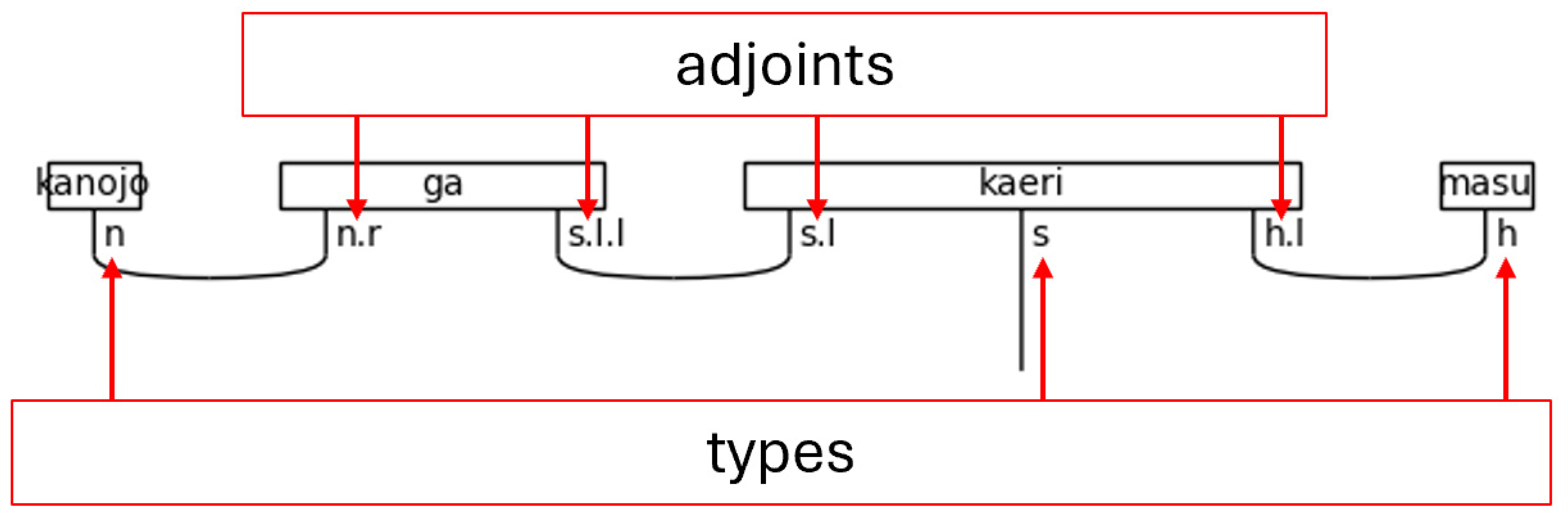
The process of creating a quantum circuit without using the BobcatParser in lambeq begins with defining types, also known as simple types. Combinations of types—called complex types—are assigned to words. After the definition of simple types, the connectivity of the grammar is specified by pairing the simple types with their left or right-adjoints. For example, the type s has a left-adjoint called s.l and a right-adjoint called s.r. The left and right nomenclature can be remembered by the adjoints relative position to the noun. The right-adjoint, for example, will always be written to the right of the non-adjoint, simple type (the base type)—i.e., n.r will always be found to the right of n. Adjoints can be chained, like s.l.l (the left-adjoint of the left-adjoint), which simply means that the s.l.l is to the left of an s.l type that completes the pair. Lastly, the grammar connections of the words are joined together using cups, resulting in a type of string diagram known as a pregroup diagram.
Figure 3.
Words and Cups in a Pregroup Diagram.
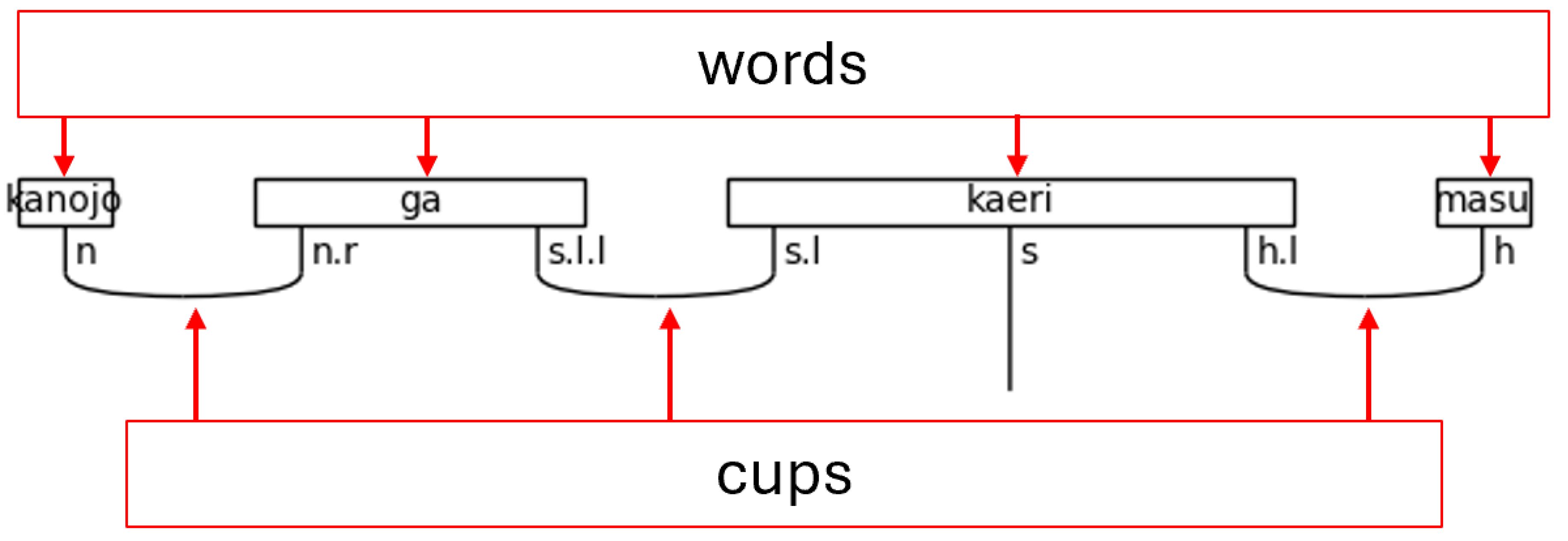
Figure 4.
Types and Adjoints in a Pregroup Diagram.
For this project, the type definitions have been separated into their own file named jp_grammar_model.py to honor the software engineering principle of separation of concerns. Because the sentence type s and the noun type n are standard types, lambeq provides them as enumerations. The honorific type h is a custom implementation. The instantiation of these types is found in Figure 5.
Now that these basic types are defined, they are combined into complex types to grammatically type words in a sentence. The remainder of the contents of jp_grammar_model.py contain the complex types necessary to model very basic Japanese grammar along with honorifics. The most critical of these complex types are those found in the predicate, particles, and honorific titles, which are attached to names or otherwise used to transform a noun into a name.
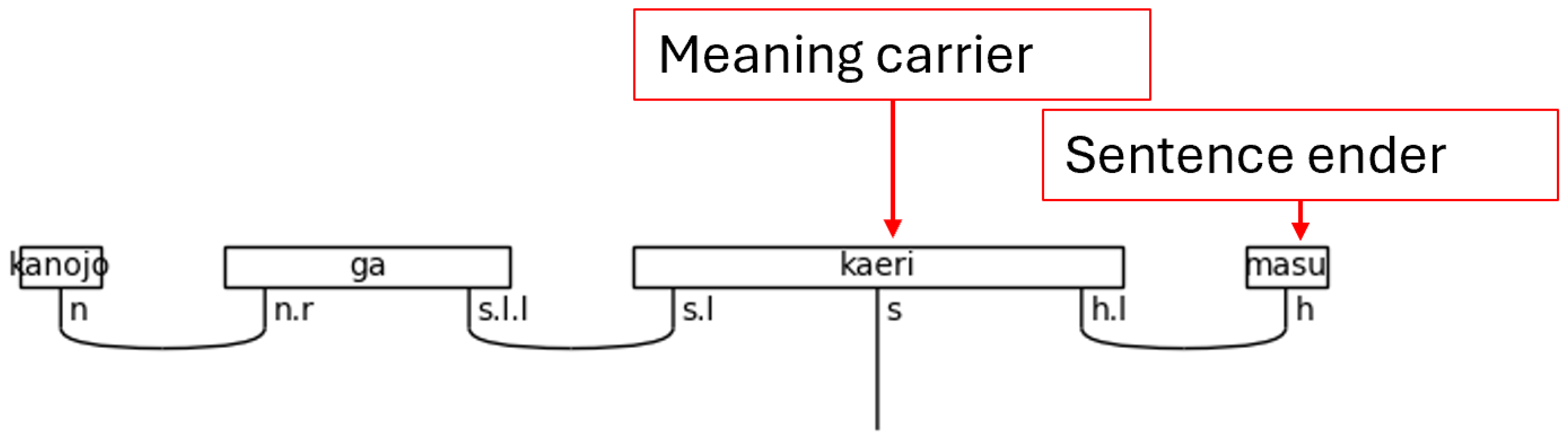
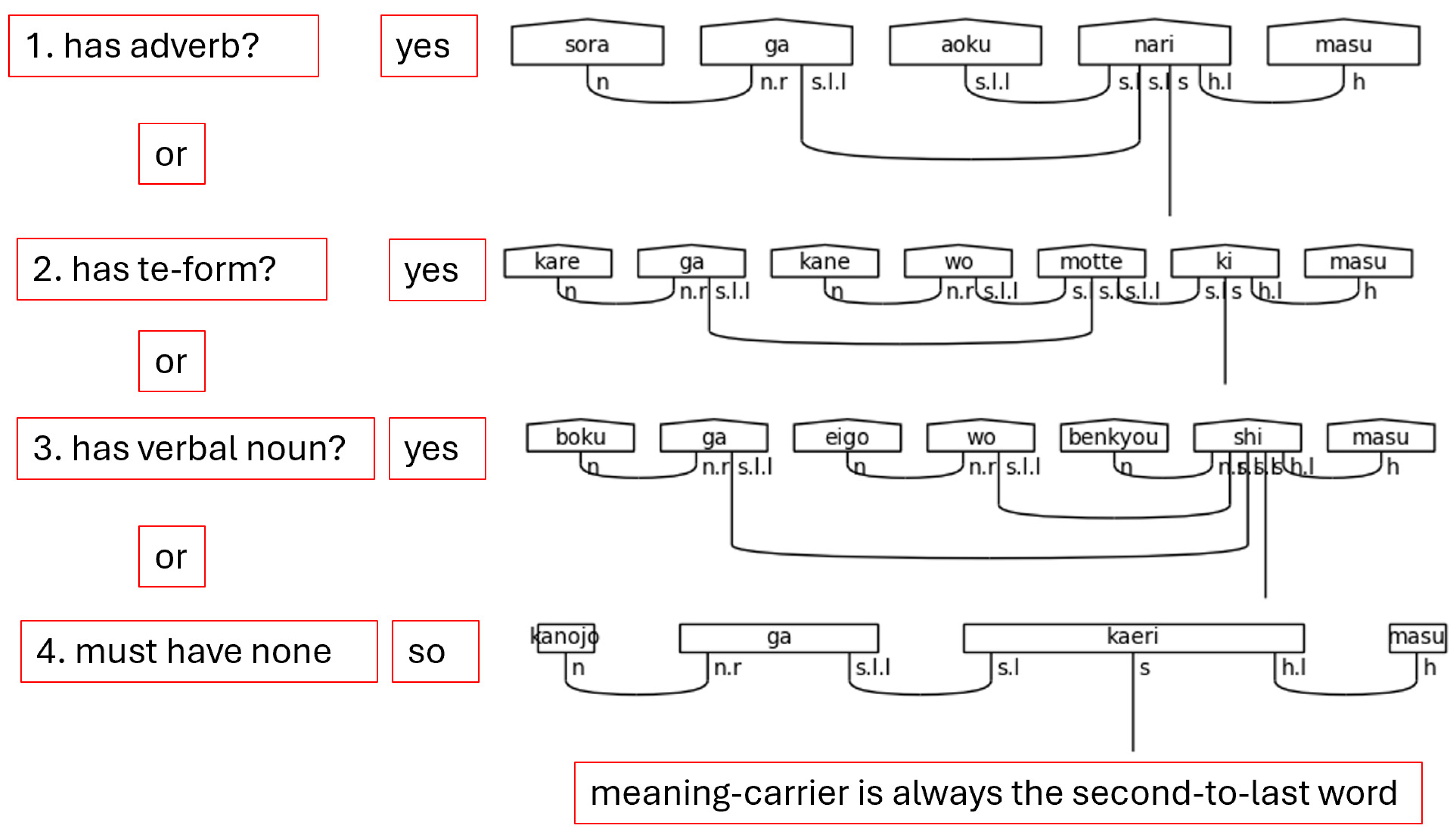
Japanese is often said to obey a subject-object-verb, or SOV, word order. This is not strictly true as the particles determine the logical, grammatical relationships between the words in the sentence. Regardless, the SOV order is often used in textbooks, and there is no flexibility in the placement of the verb or the copula in a simple sentence; therefore, SOV or OSV is possible, but a sentence will always end in with V. Specifically, in a casual sentence that is taken in isolation—topic-comment level discourse, marked with the particle は[ha], is left for future research—the final word in the sentence always carries the sentence type—carries the meaning (Dvorak & Walton, 2014). When the polite form is used, the final word instead, or additionally depending on the situation, adds in the vertical dimension of meeting—the politeness level. This means that the final word does not always carry the textual meaning of the sentence. Therefore, the grammar model must account for this when considering the predicate at large. In the discussion that follows, any grammatical type that can end a sentence is simply referred to as a sentence-ender. This is shorthand for verbs, the copula, and politeness markers. Whenever the sentence-ender does not carry the textual meaning of the sentence, the word that does will be referred to as the meaning-carrier. Again, this is a shorthand to identify the word that will include the s simple type as a part of its complex type definition.
There is one more crucial note to make regarding the meaning-carrier before continuing. The meaning-carrier is the changeling in the sentence. While it will always have an s core, the number of particles, the presence of adverbs, other verbs, or even the presence of nouns in some cases will persuade the meaning-carrier to adopt a different typing. In other words, the meaning-carrier is very much influenced by the company it keeps.
Figure 6.
Sentence-ender and Meaning-carrier in a Polite Sentence.
Consider first the casual predicate types found in Figure 7. These complex types, and those that follow, are used in the string diagram building algorithm, named diagramizerin jp_grammar_utilities.py. There will be more on that algorithm starting with the Beginning with Diagrams section that follows.
Now, the casual level of language has no honorifics, so its type definitions are the simplest. The fundamental type here is that of the casual verb, named verb_casual, because its core is none other than the s type itself. It is also worthy of note that the い[i]-adjective type is nothing more than a casual verb when it is the sentence-ender. That is shown in Figure 4 by the variable adj_i_s, where “s” means the sentence type s. Adjectives that are not found in the predicate, adj_i, modify nouns, as would be expected. They are included in Figure 4 for completeness. The presence of particles will cause the s type core of the sentence-ender to expand with one s.l type for each particle present. This is because the particle specifies the relationship between the noun to which it is joined and the sentence-ender in the casual case.
Figure 8.
Casual Verb Sentence-ender in a Pregroup Diagram.
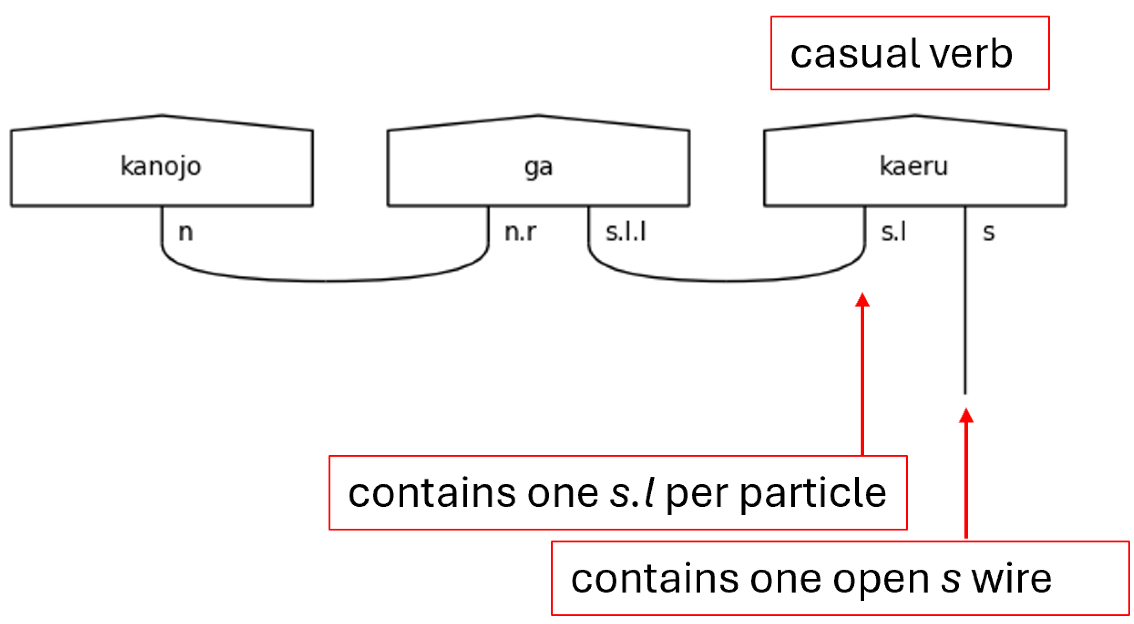
Figure 9.
Predicate Adjectives are Casual Verbs.
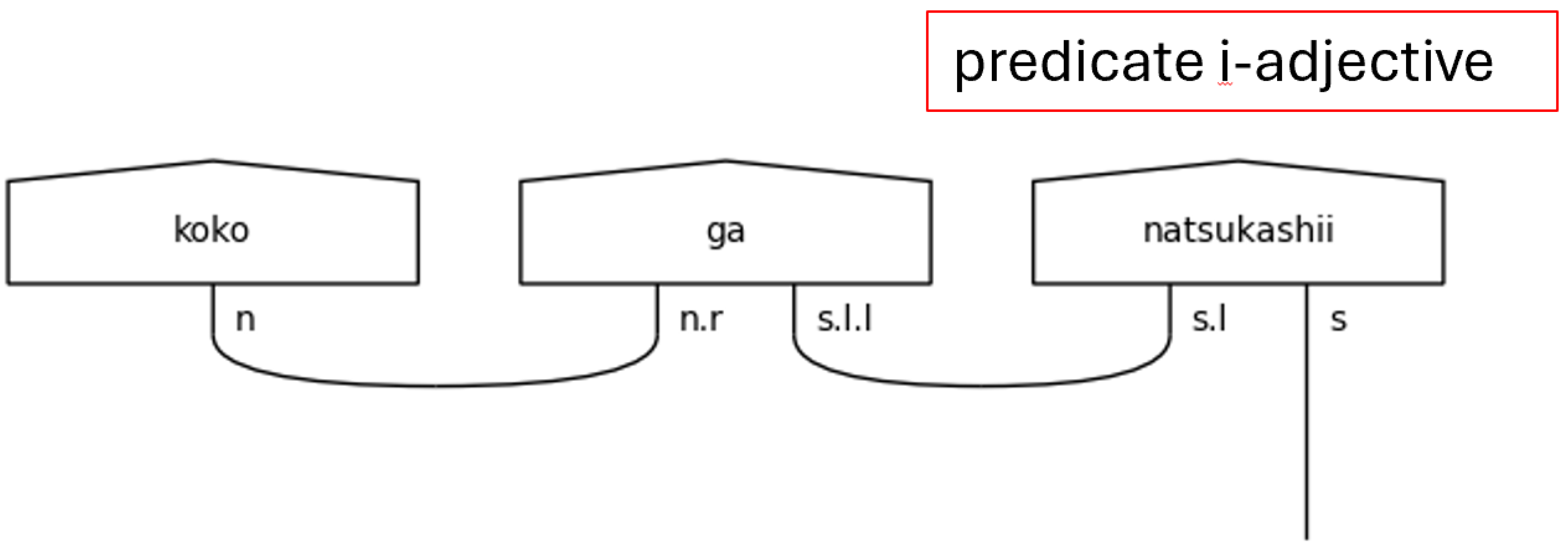
Figure 10.
Particles in Pregroup Diagrams of with Casual Japanese Verbs.
The て[te]-form is a special form of a Japanese verb that allows its meaning to directly modify the verb that succeeds it. It, in effect, allows an entire verbal clause to modify another verb. Therefore, it allows a verb to function adverbially—as a standalone s.l.l type in this grammar model. When it does this, the particle links, the s.l types, of the sentence are paired to the て[te]-form, and the て[te]-form verb itself expects another verb to succeed it and bear the sentence type.
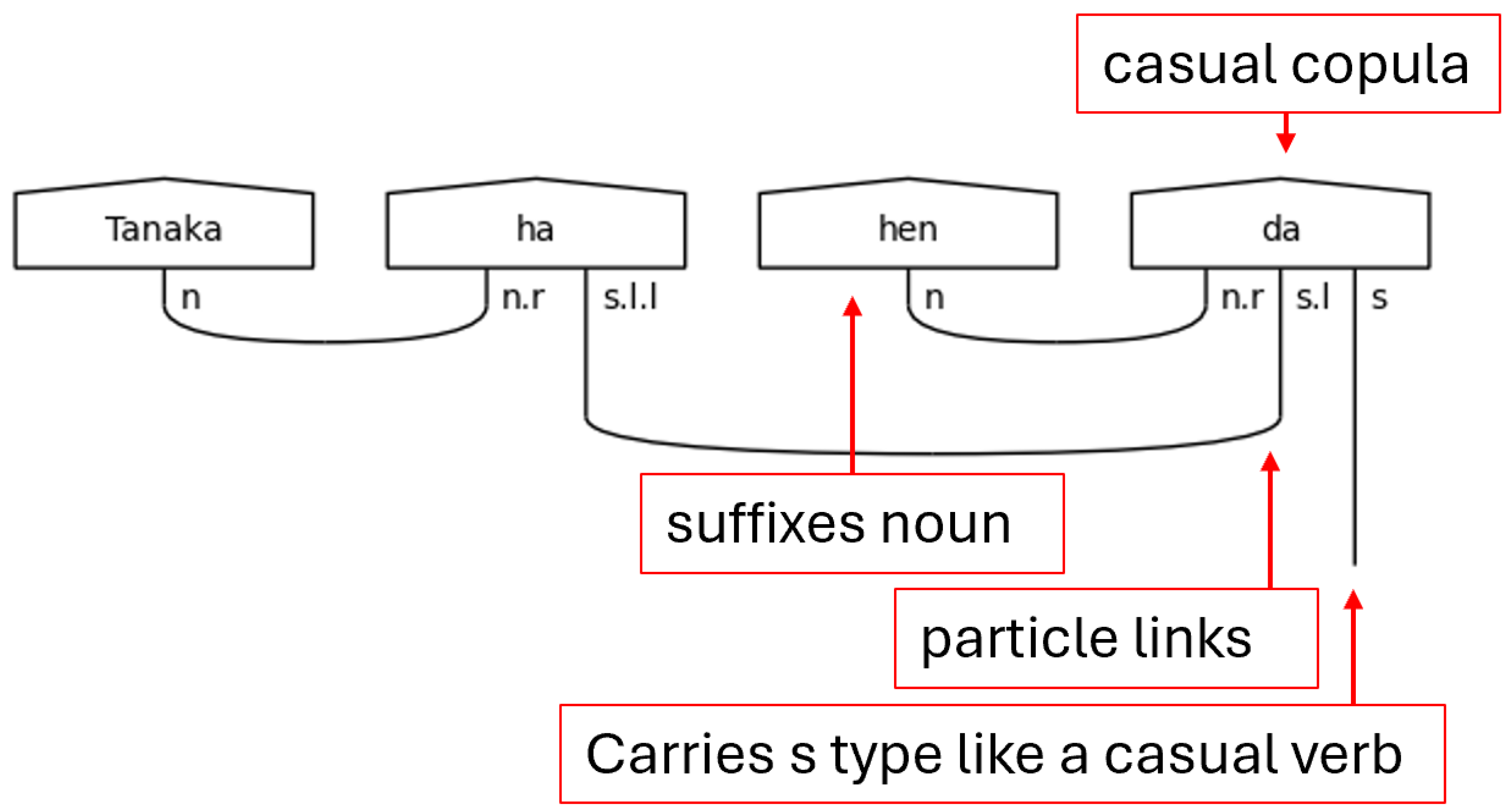
Lastly for the casual predicate section is the copula だ[da]. The copula functions strangely, at least to the native English-speaker, in that it is a statement of the equivalence of two things but is not a statement of their being. In other words, it bears the fundamental meaning of “is” without any implication of existence. The copula, then, can be thought of as an equal sign (=). Practically speaking, this means that the copula must suffix a noun like a particle, hence the n.r type on the left-side of the copula’s complex type. Otherwise, it functions like a verb. The s.l here is a stand-in for any number of particle links needed to carry the meaning.
Figure 11.
て[te]-form in a Pregroup Diagram.
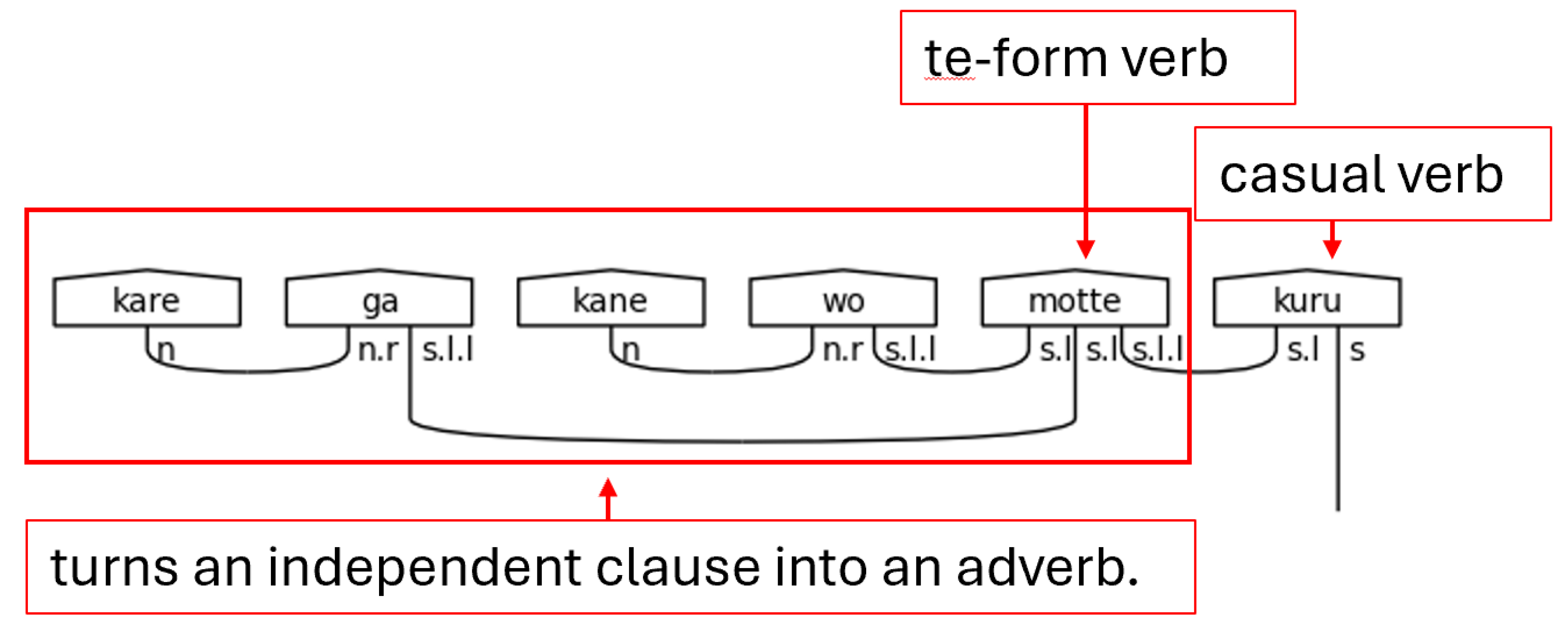
Figure 12.
The Casual Copula in a Pregroup Diagram.
With casual sentences, there is a simple pattern. The connections flow from the left to the right. In the casual sentence-ender, any noun terms, as in the case of だ[da], are defined on the leftmost side of the assignment. The particle links follow next, and the final term will always be the s term. This order always holds and will become crucial for the implementation of the diagramizer algorithm.
Consider next the polite predicate types found in Figure 13.
Everything that was true about casual verbs is also true here with two notable exceptions, both of which are caused by the inclusion of the h type. The first exception is the inclusion of the honorific type’s left-adjoint, h.l, on the left-side of s types in the connective—polite form stemmed—verb, verb_connective. The second is the inclusion of the h type on the left-side of the n.r type in the case of the polite copula です[desu], desu_n.
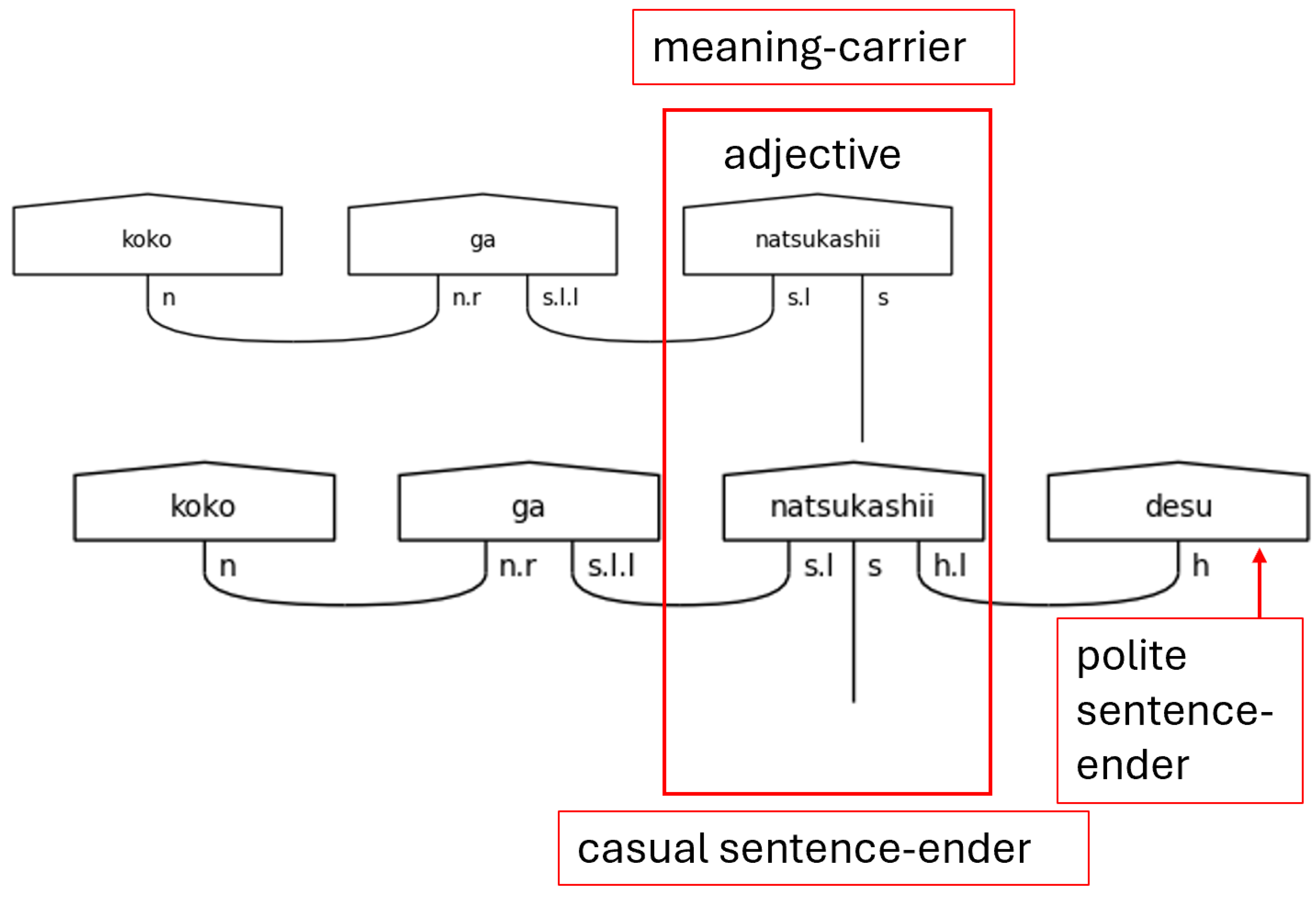
First, regarding the use of h.l, verbs in the polite form anticipate the helper verb ます[masu] to succeed them. ます[Masu] always has the type h. This, then, is the first and archetypal example of a sentence ending word that does not carry the meaning. When ます[masu]is present, the meaning is always carried by the connective form verb that precedes it. The same is also true of the predicate use of the adjective. There is no difference in the assigned types between polite verbs and predicate adjectives paired with です[desu].
Figure 14.
Polite and Casual Juxtaposition of the Same Sentence.
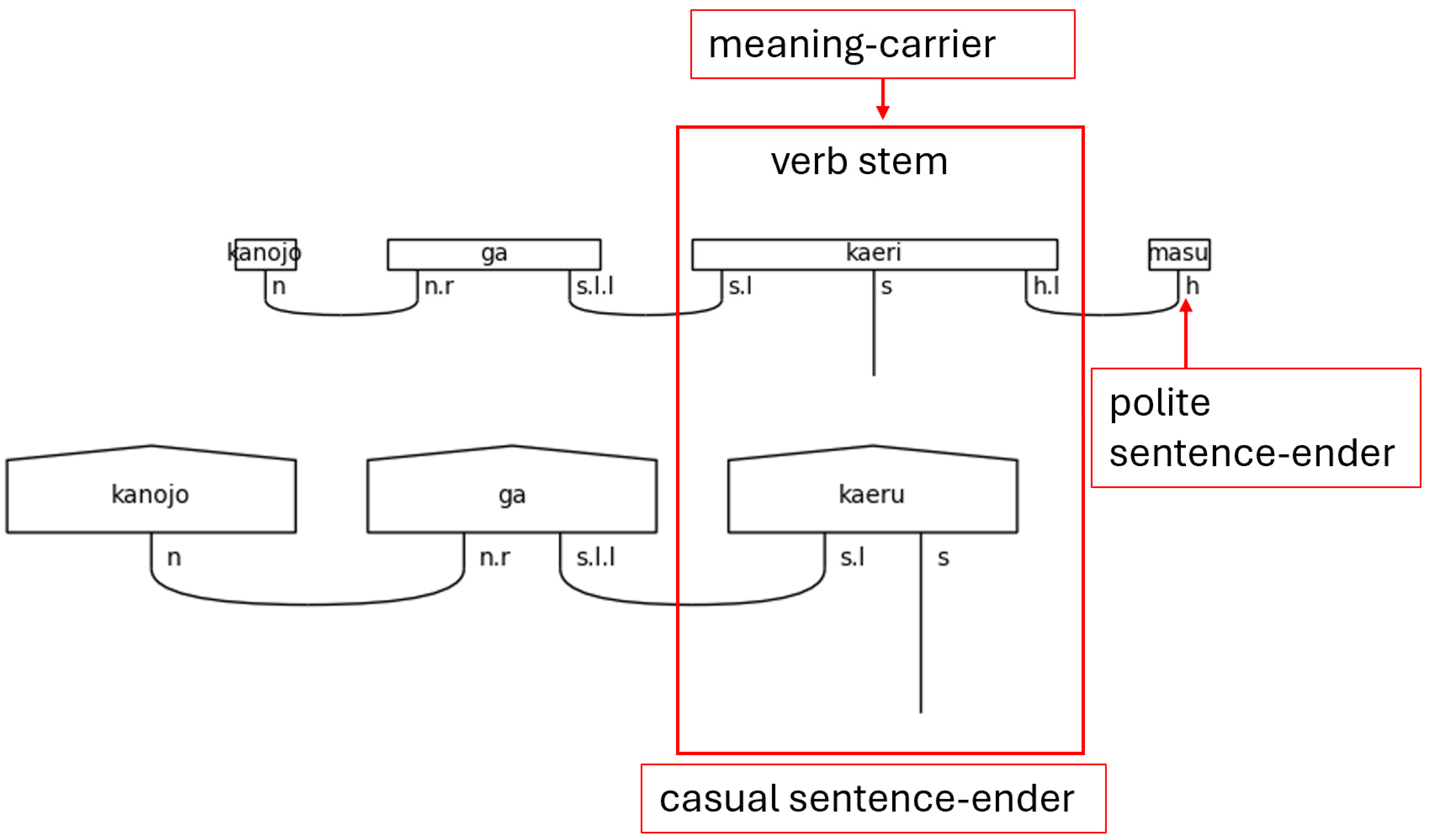
Figure 15.
Polite Sentence with a Predicate い[i]-Adjective.
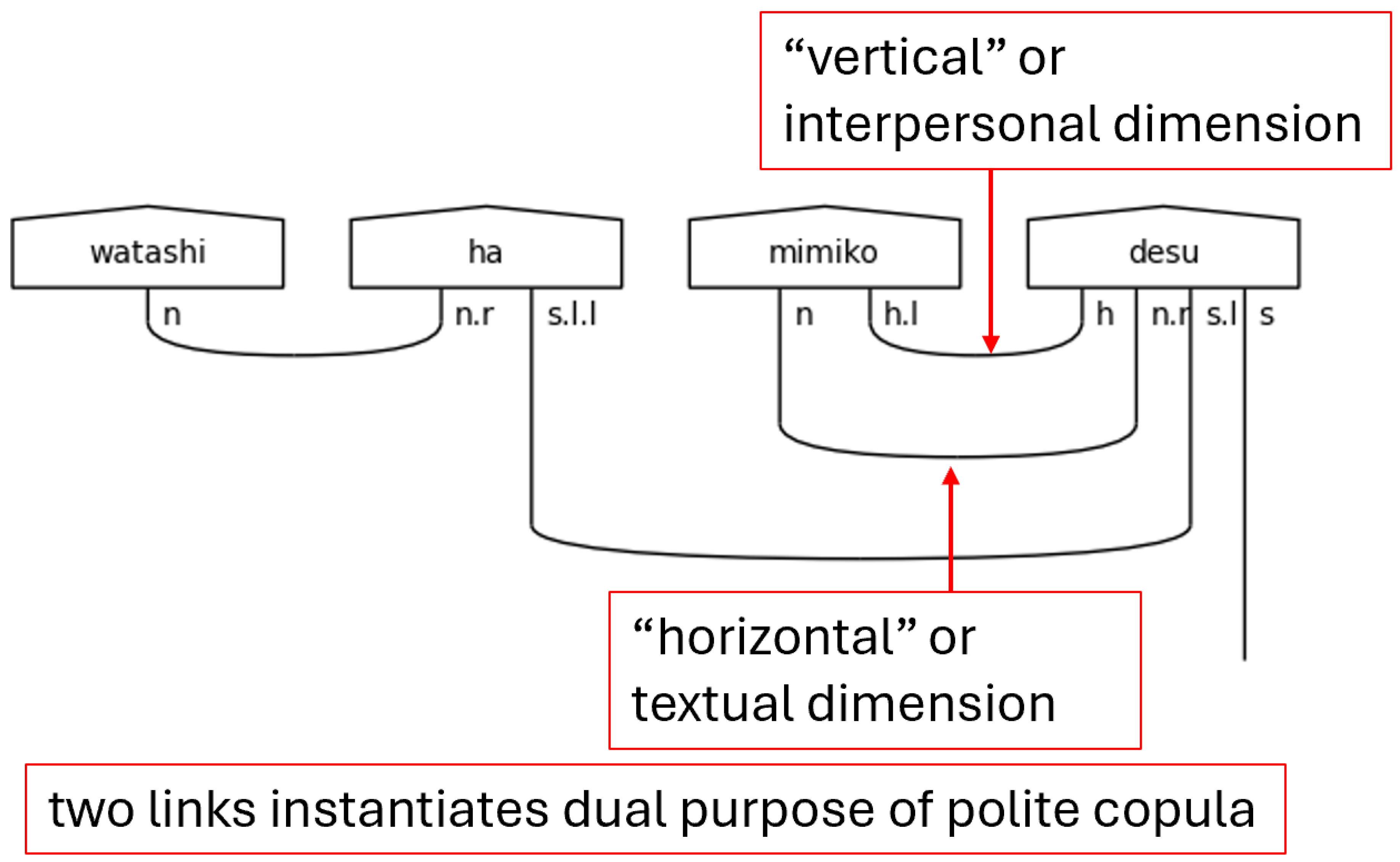
Second, the h on the left-side of n.r is a special case that occurs only with the aforesaid です[desu] in this grammar model. The result of this h is that the predicate noun that precedes です[desu]is expecting two links, resulting in the special type assigned to pred_polite_n. The use of this type means that two cups will be drawn between the predicate noun and です[desu]. The reason for this is that です[desu]is serving two purposes in the sentence. The first of these is that of the copula—the textual case of equivalence. The second of these is to mark the sentence as polite—the interpersonal case of honorifics. This dual purpose of a single word is a great example of the two-dimensional nature encoded into Japanese utterances.
Figure 16.
A Special Case: Predicate-Noun Usage of です[desu].
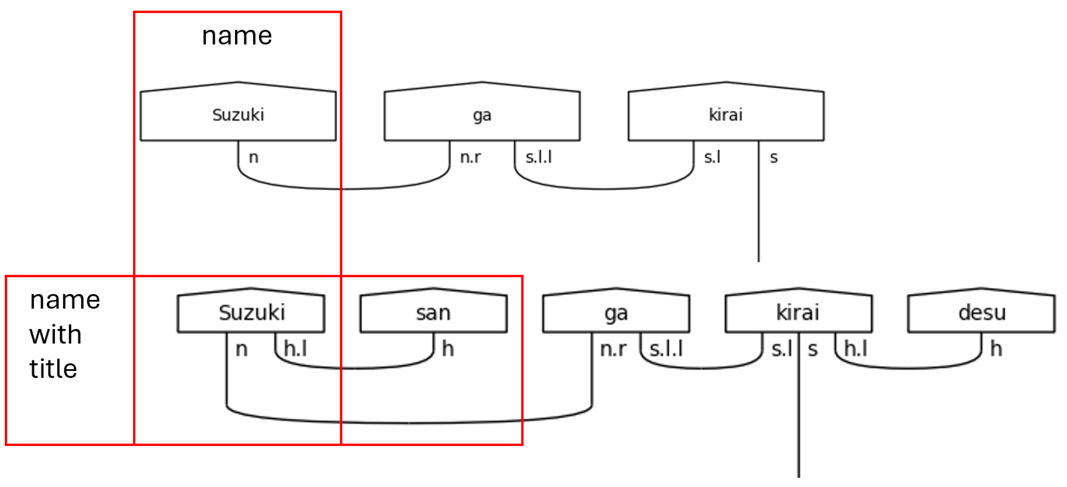
There are two more portions of the grammar model that deserve attention here. The first of these is titles, and the second is particles. In the simplest sense, titles in Japanese approximate the English titles that have fallen out of fashion in contemporary parlance. The use of the most universally recognized title, さん[san], as a suffix can be translated as “Mr.”, “Mrs.”, “Ms.”, “Miss”, or any other related term. It specifies no sex or marital status. Instead, it simply elevates the use of a name in politeness. Since this is its function, it modifies the type of the name or noun to which it is fixed. Figure 17 shows the variable assignments for titles and names.
Modification, of course, makes no sense unless there is some baseline from which to modify. In this case, that baseline is the casual name—cas_name. A name is nothing more than a highly exclusive and specific noun. It’s counterpart, the pronoun, is itself a noun that is, on the other hand, inclusive of a larger category of people and completely general. Nevertheless, these are all nouns in this grammar model because they link to other parts of speech in the same way. It is the polite name—name—that stands out as something more. While it remains a noun, it also bears an h.l, so it anticipates the title suffix that follows, and because it anticipates, it is changed. This change that the presence of the title brings on makes it a special word—a word that determines types of other words—to which the diagramizer algorithm pays special attention.
Figure 18.
Comparison of a Casual Name and a Polite Name with a Title.
Speaking of special words, now is a good time to introduce the others. Figure 19 shows them. This list is by no means comprehensive for Japanese, but it is sufficient for a first iteration of the grammar model to handle a functional variety of simple sentences.
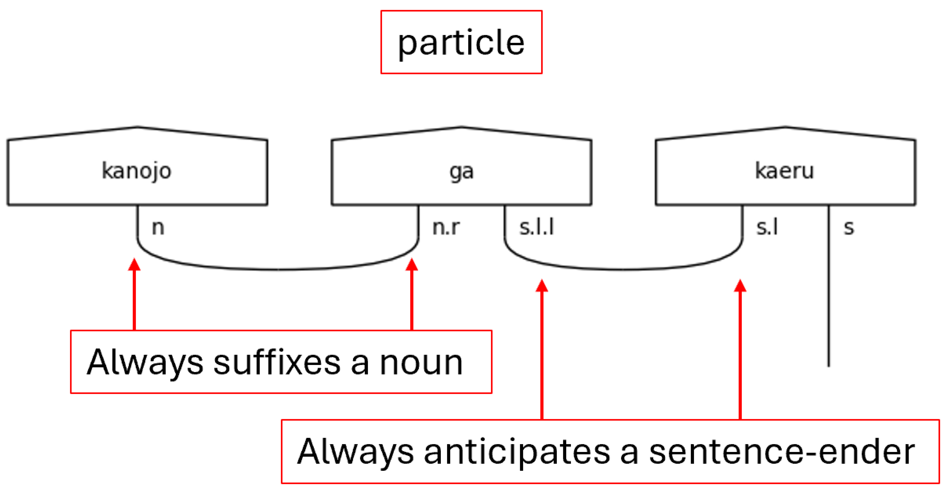
The honorific words, titles, and copula make their appearances again here in python lists, which will be used for list comprehension tasks later. For now, the new part of speech to consider is the particles, which are found in the particles list and the possessives list. In Japanese, particles can be thought of as utterances that suffix nouns and specify the relationship of the noun to the action of the verb. To use terminology familiar with English speakers, particles are words that explicitly define the subject, object, indirect object, and so on of a sentence. They also, therefore, give Japanese its flexibility regarding word order. Since their essential function is to suffix nouns and link to verbs, their position in the sentence—their indices in the ordered list of words—will be of great importance later. Figure 20 shows their type assignments.
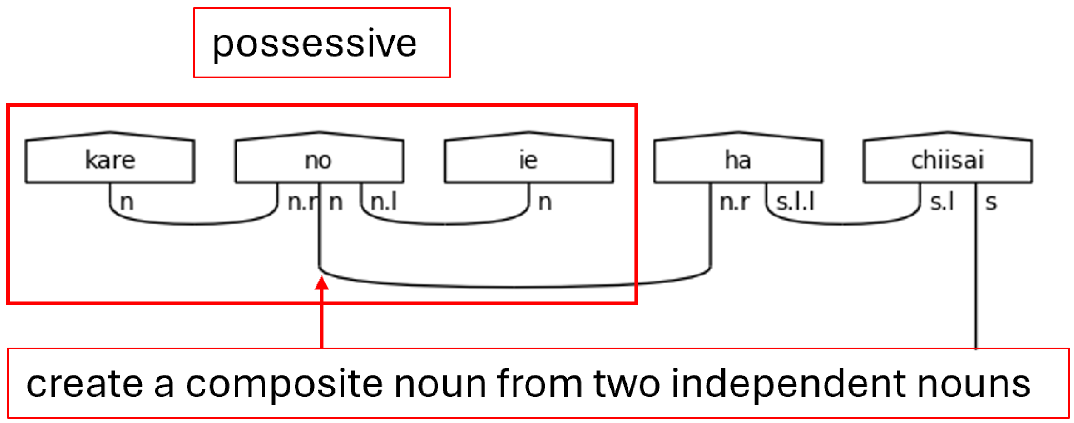
The possessive, or genitive, particle の[no] will always link two nouns together, so it is expecting a noun on its left and on its right. The simple noun type in the middle, then, remains to connect to suffixed particles. There are other uses of the particle の[no] that are not considered here as it is one of the more overloaded particles in the Japanese language. Handling the different types of の[no] in this model is an avenue of future research. The rest of the particles will always link the noun to the verb, so they carry the s.l.l type. Again, each particle in the sentence will persuade the verb to include another s.l to pair with it as in Figure 10.
Figure 21.
The Genitive Use of の[no].
2.6.3. Beginning with Diagrams
Having defined the grammar model in jp_grammar_model.py, it is time to discuss the diagramizer algorithm found in jp_grammar_utilities.py. The purpose of this algorithm is to parse a simple, proper Japanese sentence that has been tokenized into the format presented in Figure 22 and create a string diagram. That string diagram can subsequently be converted into a quantum circuit.
A note on tokenization. Tokenization is, of course, an art as well as a science. This tokenization follows the convention of using whole words separated by white space to tokenize input data for QNLP tasks, which results in diagrams with cups drawn between whole words. It also relies on romaji, which is the anglicized spelling of Japanese words. This is due to the tkinter library, on which lambeq relies in part for drawing diagrams, lacking support for properly displaying kanji and kana—hiragana and katakana—characters even when a file is encoded with UTF-8. Instead of developing a potentially time-consuming work around, the decision was made to work with romaji to avoid the issue as the display format of the text does not impact the core of the diagramizer algorithm. While the decision to use romaji makes certain tokenization decisions a little simpler, it does make it more difficult to handle certain adjectives that phonetically end with an “i” sound (pronounced like “ea” in “eagle”) with total accuracy. This will be discussed in greater detail when discussing い[i]-adjectives in Step 1.
The pseudocode. The diagramizer algorithm consists of eight essential steps.
- 5.
- Receive and validate the input.
- 6.
- Locate the indices of special words in the sentence.
- 7.
- Count the number of particles to aid in determining the sentence-ender’s type.
- 8.
- Type the predicate by identifying the sentence-ender and, if necessary, other special words found in the predicate.
- 9.
- Type all the indexed special words and then the rest of the sentence via pregroup grammar rules.
- 10.
- Create a list of sub-types to allow referencing the simple types directly.
- 11.
- Copy this list and mark paired sub-types so the algorithm will not attempt to pair previously paired sub-types again. Paired sub-types share a cup at this stage.
- 12.
- Draw the diagram.
Figure 23 shows the code. Steps of interest will be discussed in more detail as the functions performing them are introduced.
Step 1. In Step 1, input validation focuses on ensuring grammatical expectations are met rather than attempting to address every possible edge case. The grammatical expectations for a Japanese sentence rest primarily on the sentence-ender, so attention is focused there. Figure 24 shows the function.
The endings variable is assigned a tuple of valid sentence-enders in the Japanese grammar model. These only catch whole words at the end of the sentence strings, so if です[desu], ます[masu], or だ[da] is present, the sentence is assumed to be valid. This is generally true as the copula implies the subject based on the context and ます[masu] is only used in conjunction with a polite verb preceding it. That preceding verb will also imply a subject, so it will produce a valid utterance. The other validation checks are looking for the non-past verb ending “u” or the い[i]-adjective ending “i”. In the former case, the “u” could be preceded by any of the consonantal sound in Japanese and still yield a valid verb (i.e., う[u], く[ku], す[su], る[ru], etc.). In this case, romaji makes the validation check easier since checking for the “u” sound catches all the casual non-past verbal endings. The latter case requires a little more processing to ensure that the ending “i” character is not a common な[na]-adjective like 綺麗[kirei] and 有名[yuumei] by checking for “ei”. While this is not a perfect solution, as this also does not address common names, it is sufficient to handle most sentences. In this case, kanji and kana characters would be more useful as the い[i]-adjective must end with the hiragana い, which is transliterated as “i”. There is no way to detect this with complete accuracy without using the kanji or splitting the “i” off い[i]-adjectives and treating it as a separate token. Investigating these approaches is left to future work.

Table 1.
Sentence-ender Candidates and Their Validity.
| Japanese | Transliteration | Part of Speech | Translation | Valid? |
|---|---|---|---|---|
| 嫌い | kirai | い[i]-adjective | “dislike”, “hate” | yes |
| 綺麗 | kirei | noun or な[na]-adjective | “beautiful”, “clean” | no |
| ます | masu | verb | None polite verb ender |
yes |
| 持つ | motsu | verb | “hold” | yes |
| 源治 | Genji | noun | Nonename | no |
| だ | da | copula | “is”, “am”, “are” casual |
yes |
| です | desu | copula | “is”, “am”, “are” polite |
yes |
Note. A な[na]-adjective is a noun that modifies another noun using the word な[na]. It generally behaves as a noun and is, thus, considered as such here. An い[i]-adjective is a true adjective in Japanese. The い[i]-adjective and な[na]-adjective monikers are included here because they are ubiquitous in educational literature.
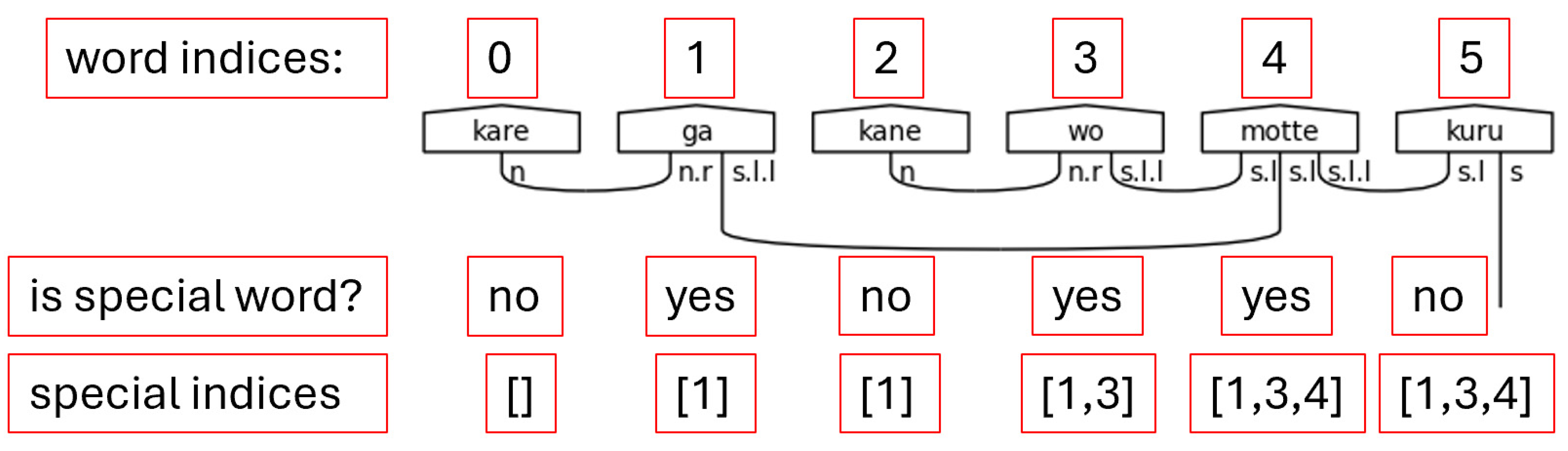
Step 2. Locating the indices of special words in the sentence is the second crucial step. While it is true that to truly understand the grammatical structure of a Japanese sentence that one must begin at the ending, it is also equally true that the ending is dependent on the presence of certain special words, namely particles, honorific words, and the copula. Figure 25 shows the function that accomplishes Step 2.
The indices are appended to lists which are themselves stored in a dictionary using the special words as keys. Each word is then enumerated, which creates a tuple of with the first element being an index and the second element being the word. If the word is found to be one of the keys—one of the special words—in the special word dictionary, the index is appended to the list associated with said key. This approach is concise and flexible enough to handle multiple occurrences of the same word in different places of the initial word list. This flexibility is required for adequately handling natural language.
Figure 26.
Finding Special Word Indices Note. The special indices are a list of lists in the code. They are shown here as a flat list for visual simplicity.
Figure 26.
Finding Special Word Indices Note. The special indices are a list of lists in the code. They are shown here as a flat list for visual simplicity.
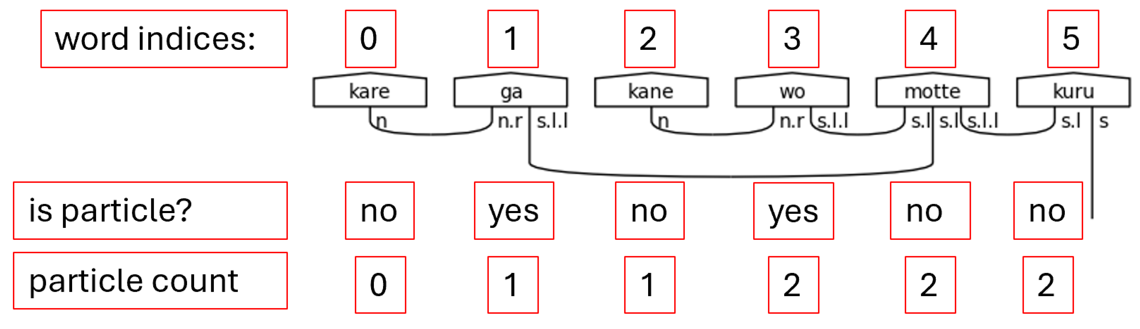
Step 3. Because the number of particles can vary significantly, it is impossible to adequately type the predicate without first counting the number of particles in the sentence. Python’s list comprehension capability, as demonstrated in Figure 27 is well suited for this task.
Given the dictionary of special words and their associated lists of indices, list comprehension allows for an easy way to calculate the sum of all the lengths of the special words that were identified as particles in the grammar model. If the special word is a particle, then length of its list is added to the accumulating sum. The final sum, then, returns the count of all particles found in the sentence.
Figure 28.
Counting Particles.
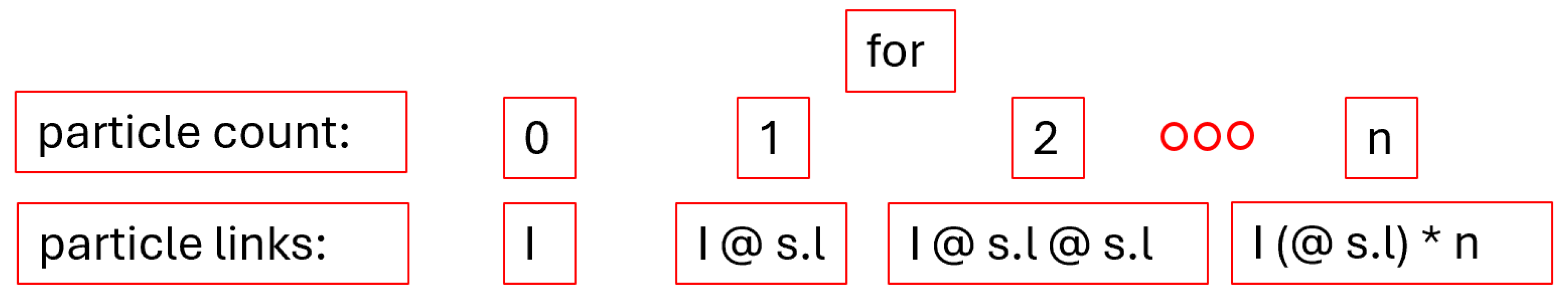
The particle count is used to build the portion of the meaning-carrier’s type called the particle links. Figure 29 shows how.
Clearly, the particle count will be the loop controller variable as each particle must connect to the meaning-carrier. A dangling particle would not provide any textual meaning to the sentence. The less obvious logic here is how to build the links programmatically. The answer is to rely on the fact that the definition of an empty Ty—the same lambeq class that was used to define the custom h type—is the identity value for types. So, by defining particle_links with an empty Ty, the calculation can be created by performing matrix multiplications—as represented by the python “@” operator—iteratively. This allows for a programmatic construction of particle links of a variable length, which in turn provides the missing information required to type the predicate of the sentence.
Figure 30.
Building Particle Links Block Visualization. Note. The “* n” operator represents repetition of the “@ s.l” string in the figure n times.
Figure 30.
Building Particle Links Block Visualization. Note. The “* n” operator represents repetition of the “@ s.l” string in the figure n times.
Step 4. Typing the predicate is a moderately complicated NLP task that relies on different helper functions depending on which sentence-ender was found in the sentence. The presence of the sentence-ender is determined by identifying which special word key returns a non-empty list as is shown in Figure 31.
The structure of the predict will differ depending on the found sentence-ender. Because of this, more complicated predicate types have been separated into an additional level of helper functions. The helper functions require the list of words and the particle links as inputs. They also leverage python’s capability to return multiple variables for readability. If there is no index for a return variable, its value will remain None.
In the case that です[desu] is found, the predicate may include a sentence-ender and a meaning-carrier. A ます[masu] can result in a much more complicated structure that includes a sentence-ender, a meaning-carrier, adverbs, て[te]-form verbs, and even verbal nouns. The casual copula だ[da] is a simple case, so no helper function is needed. It simply uses matrix multiplication to add in the particle links between the n.r and the s type. The casual い[i]-adjective case is also simple. It behaves as a casual verb but ignores the possibility of adverbs and て[te]-form verbs in this model. Both the だ[da] case and the い[i]-adjective case do not require a meaning-carrier as the sentence-ender itself will carry the s type. Lastly, the case of non-past casual verbs requires its own helper method. It returns the same values as the ます[masu] predicate except it does not require a meaning-carrier. This is a common pattern. The polite versions of sentences typically have a meaning-carrier that is distinct from the sentence-ender—with the notable exception of です[desu] used with a predicate noun. Casual sentences do not distinguish between the two. Again, this is evidence of the vertical dimension of language because of the dual functionality of です[desu].
Beginning with です[desu], the helper functions are listed in the following figures and discussed in the following paragraphs. Figure 32, then, is first.
It is first worth noting that this helper method shares the same limitations as the input validation code found in Figure 24, and it also ignores names. One possible way of adding in support for names is to create a list of common names and use it as a filter. Since that is beyond the scope of this initial version of the model, properly handling names is left to future work. The if-statement here is designed to determine whether the です[desu] is preceded by an い[i]-adjective or a predicate noun by using two-dimensional list syntax on the list of words. The left set of brackets is selecting the second to last word in the list. The right set of brackets is selecting either the last character or a slice of the word containing its last two characters. The logic here is an excellent example of how です[desu] functions in both the honorific sense and in the logical sense. In the case of an い[i]-adjective, です[desu] functions purely honorifically. It carries only h type just as ます[masu] does. The direct consequence of this is that the meaning-carrier is the い[i]-adjective that precedes です[desu] in the sentence. Now, in the case where the preceding word is not an い[i]-adjective, it will be a predicate noun. In this case, です[desu] will carry the meaning—carry the s type. This is the one case in this model where it does not hold that the cup count will be word count minus one. In this singular case, the cup count will equal the word count.
Figure 33.
Typing です[desu] Visualization.
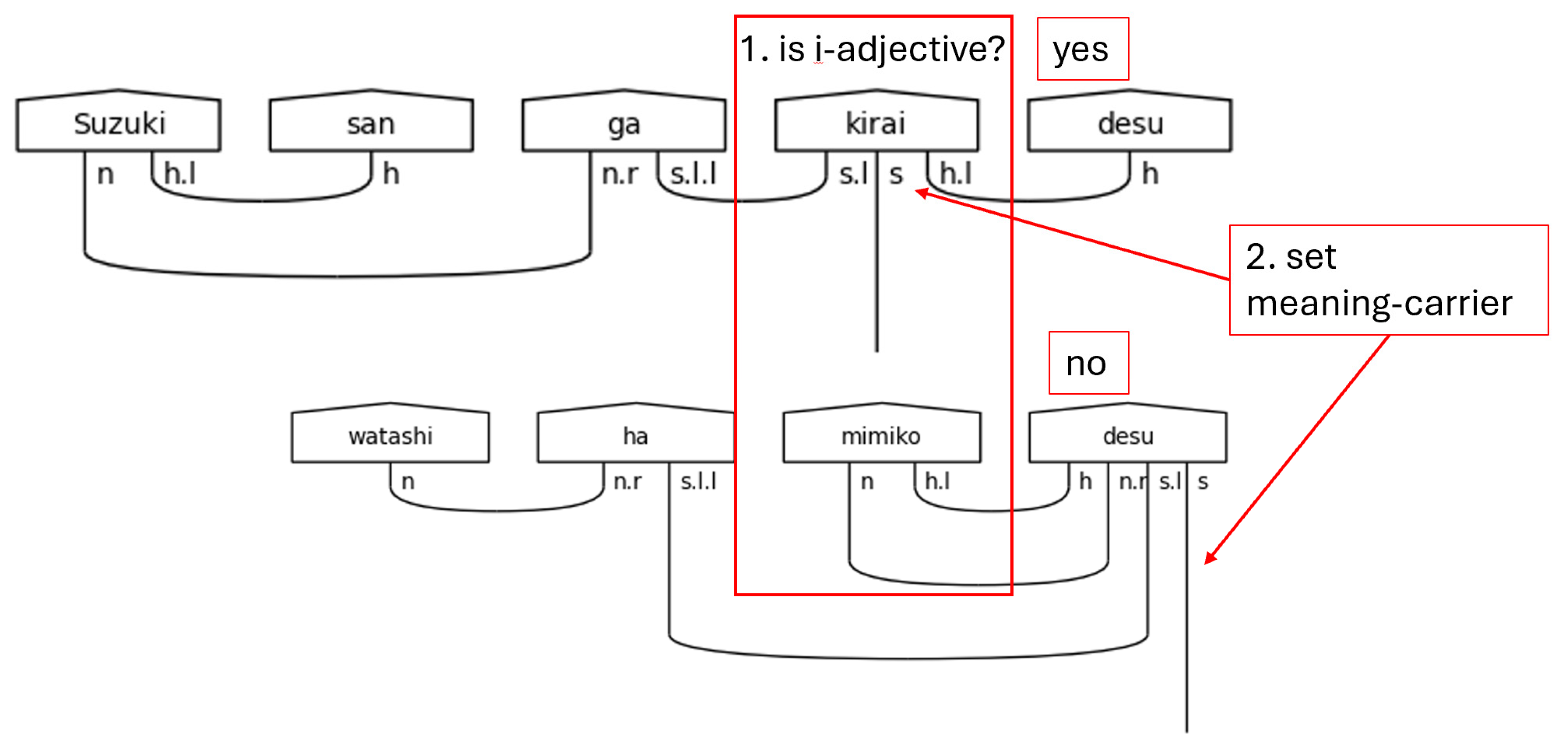
Figure 34 shows the code used for typing a ます[masu] predicate.
The function accepts the list of words and the particle links and begins its work with calculating the word count. The word count is then assigned to a variable and used to find indices for discovered adverbs and て[te]-form verbs in the predicate. The next step is to assign the sentence-ender as ます[masu]. The primary work of the method then is to determine what type the meaning-carrier word should have based on the textual clues of its preceding neighbor.
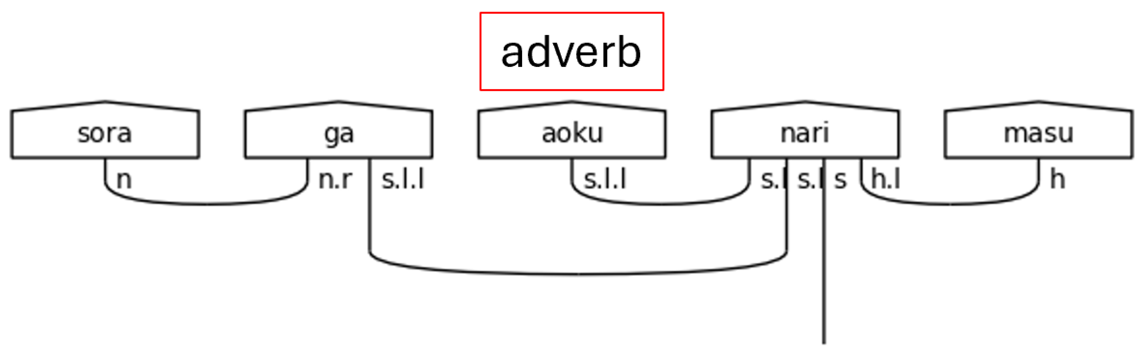
Japanese adverbs come primarily in two forms. The first is akin to the な[na]-adjective in that it is a noun suffixed with another word, in this case the に[ni] particle. Fortunately, this case is already handled in this model by the generic particle typing. Since に[ni] is a particle, the noun will be linked to the verb and no extra processing is required. The second is derived from い[i]-adjectives by changing the い[i] ending to く[ku]. This is a very regular part of the language, so finding a “ku” in the third to last position of a sentence in standard SOV order means finding an adverb. The algorithm assigns the meaning-carrier’s type with an additional s.l to resolve the adverb, and then it marks the adverb’s index so that it may be typed later.
Figure 35.
Japanese Adverb in a Polite Predicate.
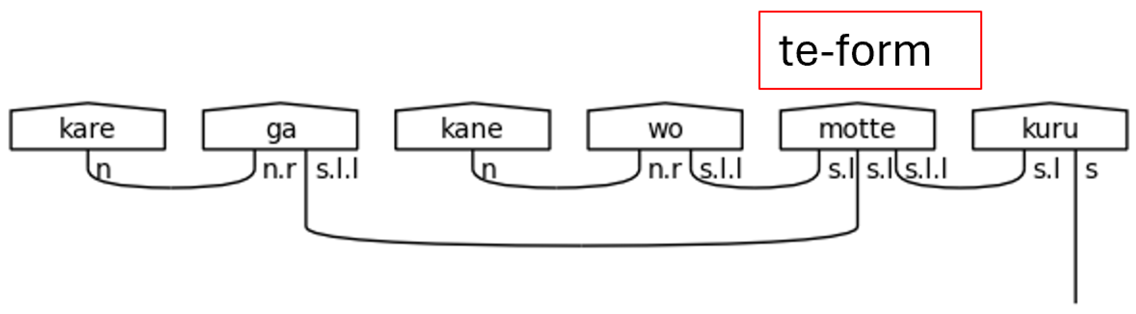
The て[te]-form is a specialized verb form that is used for a variety of reasons in Japanese. The grammar model presented here handles when the て[te]-form functions adverbially, meaning the entire clause that links to the て[te]-form verb is subsequently linked to the meaning-carrier verb. This has the notable effect of removing the particle links from the meaning-carrier onto the て[te]-form verb, which gives the effect of modifying the meaning of a verb by an entire clause.
Figure 36.
て[te]-form in a Polite Predicate.
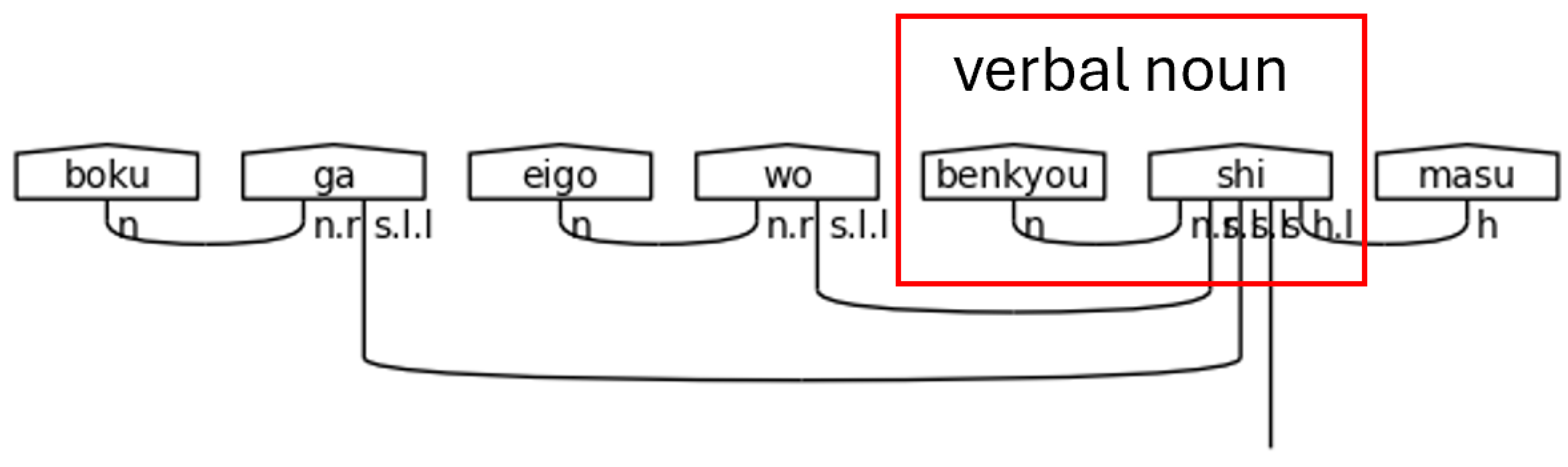
Verbal nouns, or noun-verbs, refer to nouns that receive a verb directly suffixed onto them without having a particle as a buffer. In polite Japanese, the most common of these verbs is します[shi-masu], meaning “do” or “will do” in the non-past form. By suffixing します[shi-masu] to a noun, it simply means doing the action of the noun. Verbal nouns require an n.r type in the meaning-carrier since there is no other particle present to link the noun to the meaning-carrier し[shi].
Figure 37.
Verbal Noun Condition in a Polite Predicate.
The final path in the code for the ます[masu] ending is the simple case. There are no additional words that modify the meaning-carrier or any special endings. The particle links, sentence type, and h.l type are assigned to the meaning-carrier and the algorithm proceeds on to the next step.
Figure 38.
Logic Visualization for Typing a ます[masu] Predicate.
Next, Figure 39 contains the logic for typing a casual sentence, which mirrors that of a polite sentence.
Figure 39.
Typing a Predicate with a Casual Verb. Note that it follows the same flow as the ます[masu] predicate without the added dimension of the honorific type. Additionally, since the word ます[masu] is not present in casual sentences, the sentence-ender and meaning-carrier are always the same word—the final word in the sentence. This causes the word list indices to be incremented by one in the casual case shown in Figure 39. Adverbs, て[te]-forms, and the casual verbal noun する[suru] are all accounted for. Extending this implementation to account for more complex predicates and generic verbal nouns is left to future work.
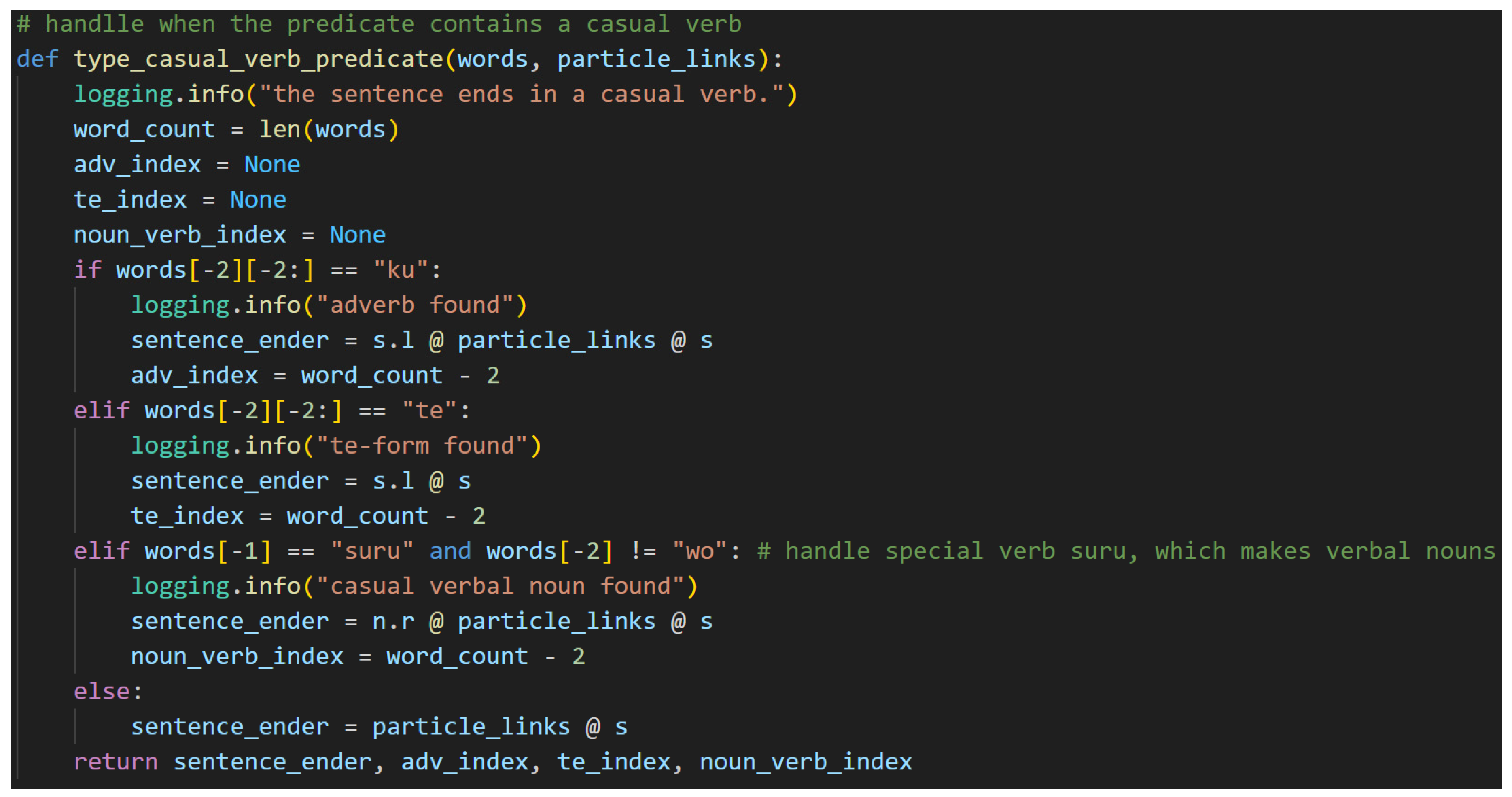
Figure 40.
Verbal Noun Condition in a Casual Sentence.

Step 5. The fifth step consists of typing the indexed special words, including any adverbs, て[te]-form verbs, and verbal nouns, along with the rest of the sentence. The first four steps have been preparing for this one. After this step, the entire sentence will be typed. The code for this step is larger, so the typing of particles and other indexed words are separated. Figure 41 covers the former case, and Figure 42 covers the latter.
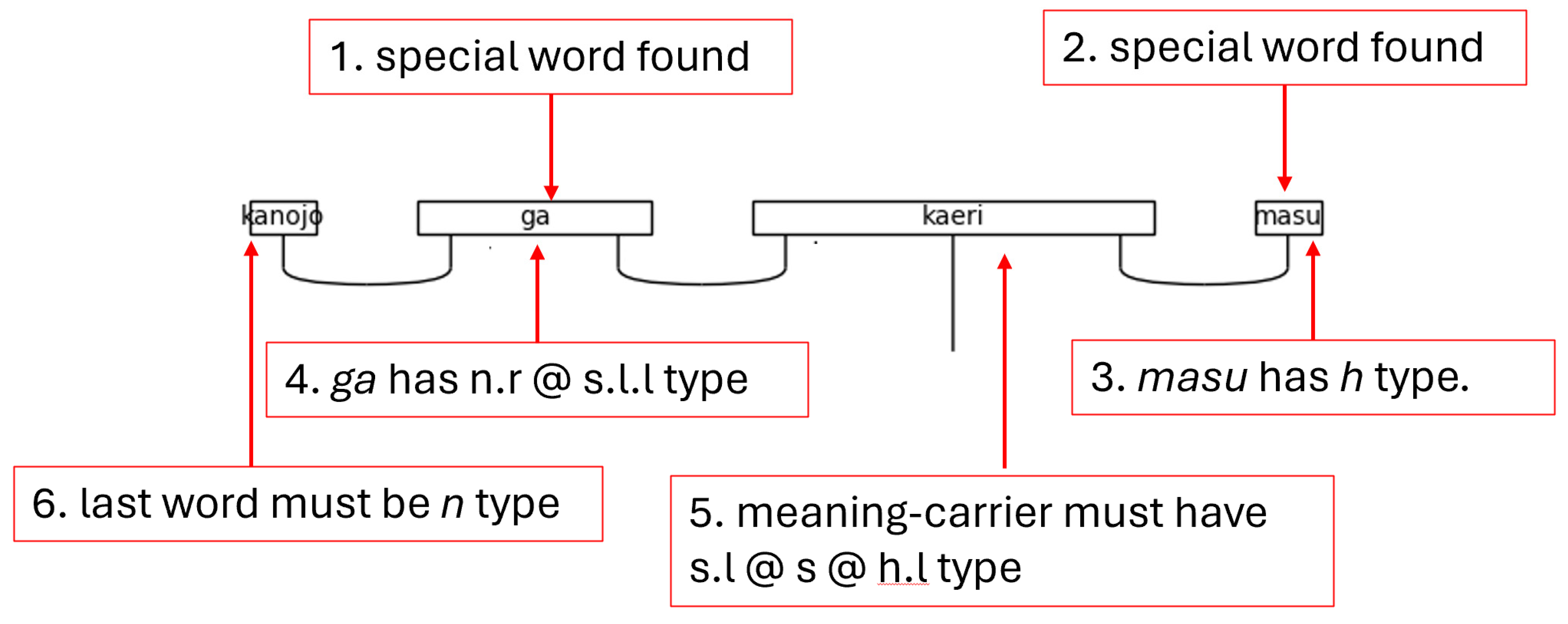
Note that the order of assignment of types in the algorithm is intentional. Like all things in Japanese, the assignment of types begins at the end. The words that are directly linked to the sentence-ender—the meaning-carrier, if present, or predicate nouns—are typed next. The rest of the predicate follows. Titles and names are handled next, followed by the possessive particle の[no]. The final portion handles the particles. This order allows for the appropriate assignment of types without overwriting. More details follow as the specific if-statements in the algorithm are addressed.
The function begins by calculating the word count and then defining a new list filled with Nones that is the same length as the word count. This new list is called types, and it will hold all of the types of the words in the original input sentence such that the word and type are matched by common index, i.e., words[1]’s typing is stored in types[1]. As types are assigned, therefore, they will be added into the types list.
The first two checks in the logic look at the sentence-ender and the meaning-carrier. If either is assigned, or not None, then the type generated during the typing of the predicate is assigned to the appropriate index in the types list. Otherwise, the assignment is skipped. These checks rely on None being “falsy” in python, meaning that None evaluates to False in a Boolean context.
The predicate noun usage of です[desu] follows. The if-statement specifically checks not only that there is a です[desu] present but also that the predicate noun version of です[desu]’s type is in the sentence_ender variable. Now, this check is the first instance of an indexed special word being used to type a word that is grammatically linked to it, meaning the index of the sentence-ender is decremented by one to point at the predicate noun. Its type, then, is assigned as an offset from the special word です[desu]’s index. The inner if-statement here is confirming that the word has not been previously typed. It, therefore, prevents later type assignments from inadvertently overwriting previous ones. This is critical for assigning the types of the non-indexed words and is a recurring pattern. The index of the casual copula, だ[da], is used to type the noun to which it is suffixed in the same—though simpler since no h.l type is required—way.
て[Te]-form verbs, adverbs, and verbal nouns are special words, so their types are assigned directly in this function. They are critical for typing the predicate, but they are not useful for discerning the types of any words in the subject. It is worthy of note here that the て[te]-form verb is assigned the particle links during this step, if present.
If titles are present, they are handled next. These can appear in the predicate but are more often found in the subject. Regardless, the algorithm here handles both cases. First, it assigns the title type to each indexed title. It then performs a list boundary check to ensure that the title is not the first word in the sentence. This should not occur since it is not proper Japanese, but safety checks are always preferred. While checking for the list boundary, the code also confirms that the title’s preceding word type is currently None to prevent overwriting. If both of those checks pass, then the preceding word type is assigned as a name, which is an n @ h.l. It is a noun that expects to be suffixed with an honorific.
The possessive particle の[no] is next. This is a unique case in that it turns a noun into an adjective while remaining a separate word. This means that the の[no] is expecting a noun on the left and a noun on the right. It, therefore, assumes the type n.r @ n.l. This, then, will link to nouns together so that the first noun modifies the second. This assignment is done by using the special word index of の[no] and offsetting to type the other two nouns. Because this is a unique case, the if-statement must check for bounds and None on both the preceding and succeeding word. When one of these cases pass, then it is assigned the type n.
Lastly, the particles are handled in Figure 42.
Figure 42.
Typing Indexed Words and Their Grammatically Related Words, Part Two.
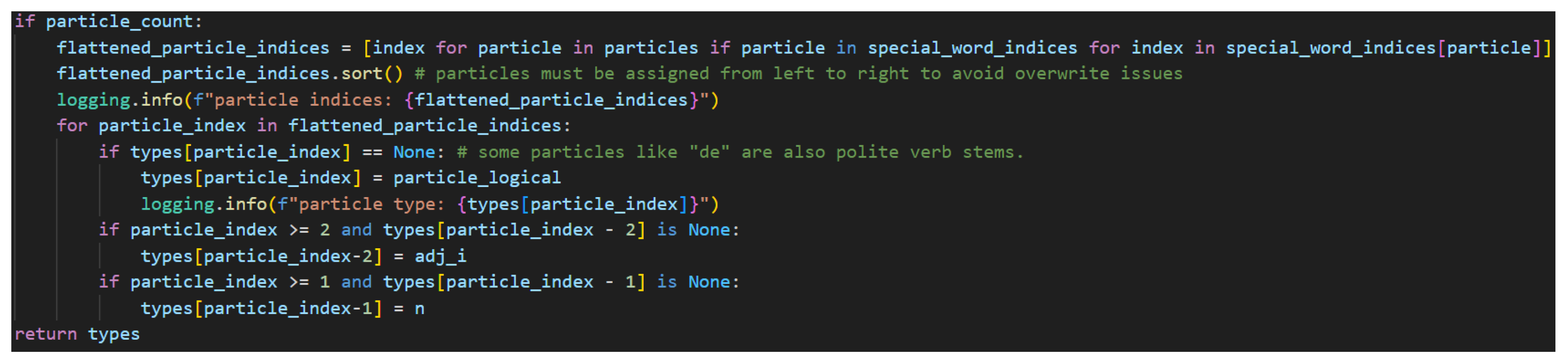
If particles are present, there will be a particle count, so that check is used to control this code. Particles require unique processing since the code has been written to track each particle in the model independently. While this is not strictly required, it is more extensible for those desiring to explore more complex typing that differentiates between the particles since they accomplish different things and serve different purposes in Japanese grammar. This code then, must flatten the particles into a one-dimensional list from the list of lists. List comprehension allows for a concise way to flatten the lists by checking for all the non-empty lists and returning their index values into a new list.
The diagramizer algorithm relies heavily on the fact that assignments must be made from left to right. This is a hard and fast rule. If assignments are done out of order, there are many instances where typing will fail to produce the correct result. Therefore, this flattened list must be sorted so that particles are typed in ascending order by index. After sorting the list, the algorithm checks to confirm that the particle index is a None type to confirm that the particle has not already be assigned another value. This is because some particles, like で[de] are also polite verb stems—meaning-carriers. This guarantees that a polite verb stem will not be overwritten with the particle type of n.r @ s.l.l.
Next comes the assignment of offset words. The particle check is reserved to the last place because it also determines which words are adjectives. It is clear from the typing of the particle that the preceding word is a noun, so it will assign that type. The, perhaps, less obvious trick here is that if there are still unassigned types at this point in the processing, they must be adjectives. Therefore, by decrementing the particle index by two, adjective types may also be assigned. The model, then, can account for adjectivally modified nouns that are suffixed with a logical particle. At this point, the function returns with a filled and ordered list of sentence types.
Figure 43.
Example of Typing Sentences Based on Special Word Indices.
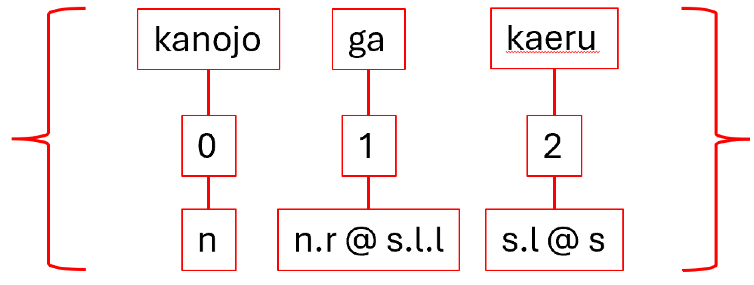
All that remains of Step 5, then, is to type the completed sentence. Recall that the list of types and the list of words are aligned so that words in the word list and types in the type list share a common index value. This fact is leveraged in the sentence typing function shown in Figure 44.
To this point, the word and type values have been assigned to lists. Now, this function takes those lists assignments and instantiates them as lambeq Words as follows. Python’s zip function takes two lists that share a common index logically and concretizes them into a dictionary—a map. This makes that logically shared index a real and actionable hook in the code. The function then iterates through each word and type, instantiates the lambeq Word, and then appends those values into a new list of lambeq Words. Once the Words have been instantiated, they can be associated with one another using morphisms, which will enable the building of string diagrams. More on that process follows beginning in Step 6.
Figure 45.
Using a Dictionary to Map Words to Types Via Common Indices.Note. The casual version of this sentence is shown for simplicity. Also, to clarify, the indices are shown in the middle row between the words (top) and types (bottom).
Figure 45.
Using a Dictionary to Map Words to Types Via Common Indices.Note. The casual version of this sentence is shown for simplicity. Also, to clarify, the indices are shown in the middle row between the words (top) and types (bottom).
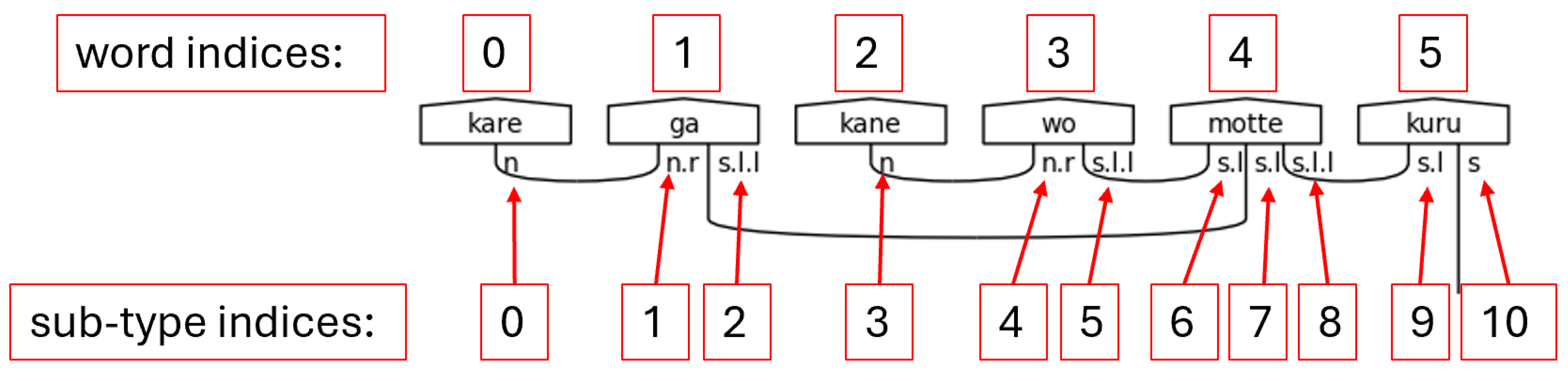
Step 6. After the lengthy, complicated indexing and list building activities of Step 5, Step 6 is a walk in the park. Be that as it may, it is critical to the success of the algorithm and easy to overlook. Based on the types appended into the types list, a new list of sub-types, sub_types, must be created. Figure 46 shows this line of code.
This single line of code is concisely combining three separate operations before assigning the sub-types into the new list. The first of these operations is casting the type as a string. This allows for the second step, which is joining the strings together into one long string using the python matrix multiplication operator—@—surrounded by spaces via the join method. This join symbol is used because it is the same symbol that is joining all the sub-types in the complex type held in each list item. By joining with this same symbol, then, the larger string will have a uniform separator between all sub-types. The third and final step, then, is to split the newly built string of all types separated by the matrix multiplication operator into a new list made up entirely of simple types. This list enables the construction of morphisms, or cups, in Step 7, which is the second major processing step of the diagramizer algorithm.
Figure 47.
Sub-type Indices Visualization.
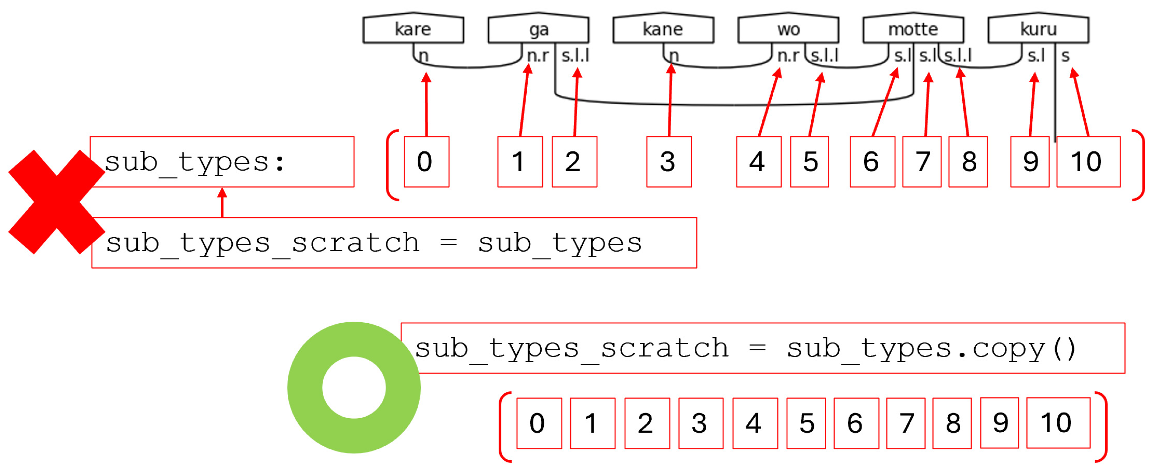
Step 7. The seventh step begins with copying the newly created sub-type list. It then proceeds to connect sub-types with cups and to mark completed pairs as matched. This work is split into two main functions. The first of which is shown in Figure 48.
This list copying function leverages python’s list and dynamic typing capabilities. First, the method copies the sub-type list. This is important because a simple assignment of the sub-type list to another variable will create a reference to the original sub-type list. Any operation, therefore, taken on the new variable is modifying the same values referenced by the original variable, which would result in an error during later processing.
Figure 49.
Passing By Reference Yields an Error. Pass By Value Instead.
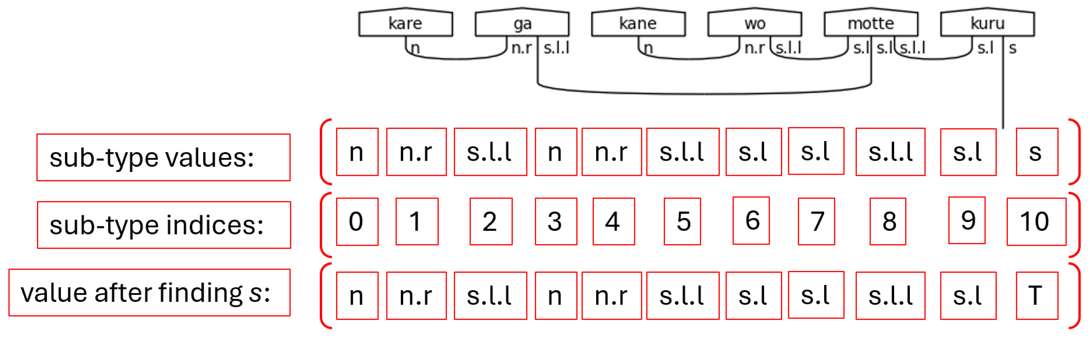
The dynamic typing capability is leveraged after attempting to find the s type in the sub-type scratch list. Once this type is found, it's value is updated to True, meaning it is considered already paired. This excludes it from the processing of the build_morphisms function. For clarity’s sake, the s type represents the only wire in a pregroup diagram that is not connected to another type with a Cup. This is the requirement for a sentence to be considered grammatically correct; therefore, it is marked True to preserve said requirement. Fortunately, the ability to reassign the value from a string to a Boolean in python allows the algorithm to mark connected pairs of sub-types logically.
Figure 50.
Sub-type Scratch Values after Marking S as True Note. Here, “T” is shorthand for python’s True Boolean value.
Figure 50.
Sub-type Scratch Values after Marking S as True Note. Here, “T” is shorthand for python’s True Boolean value.
Now that the sub-type list has been copied and the s has been marked, it is time to begin the second major logical section of the algorithm, which is responsible for connecting the sub-types with Cups—defining morphisms. The function is found in Figure 51.
Constructing morphisms, also known as drawing cups, is the process of connecting pregroup types with their adjoints, which effectively simplifies them out of the larger calculation. In the end, again, only the s base type should remain unpaired.
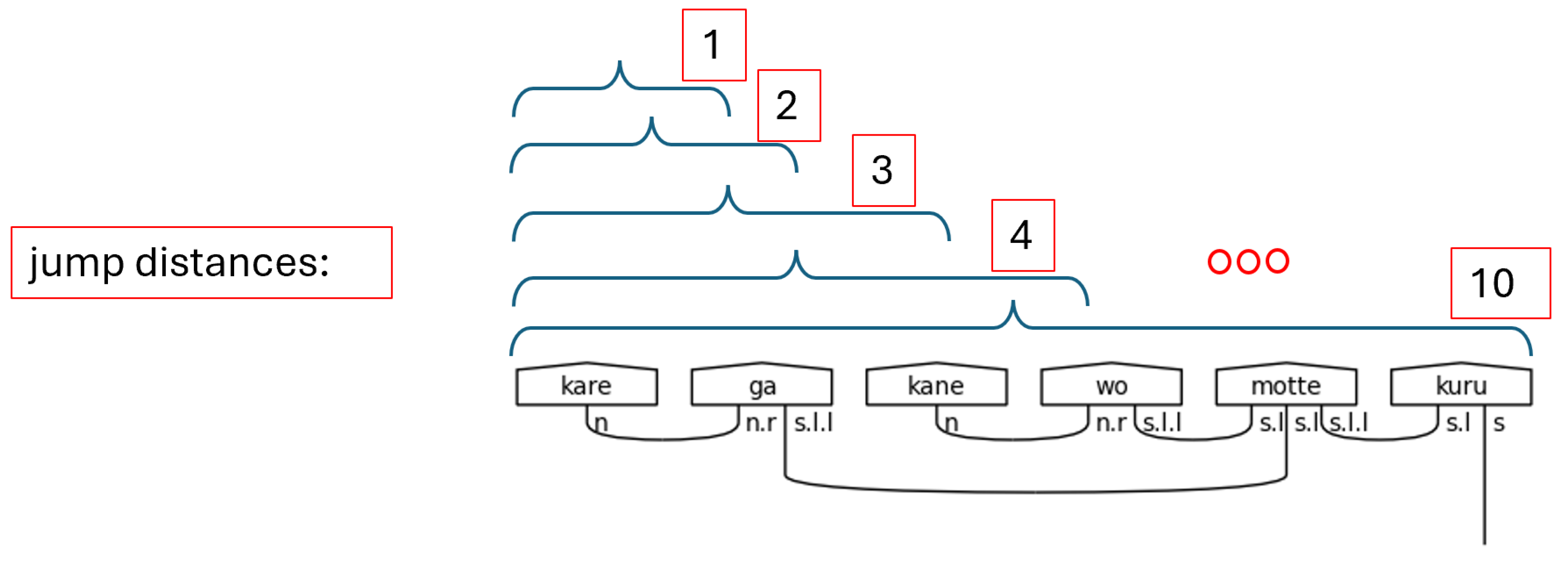
The algorithm begins by collecting the length of the sub-types scratch list. It then defines a new empty list that will hold the morphisms—the Cups in this case. The main logic of the algorithm requires nested loops, a for-loop inside of a while-loop. The outer while-loop is controlled by a counter that increments after the completion of an entire pass of the inner for-loop and by the contents of the sub-types scratch list. In the former case, the jump distance is passed to a helper function along with the sub-types count to confirm that the jump distance will not index beyond the maximum boundary of the list, as detailed in Figure 52.
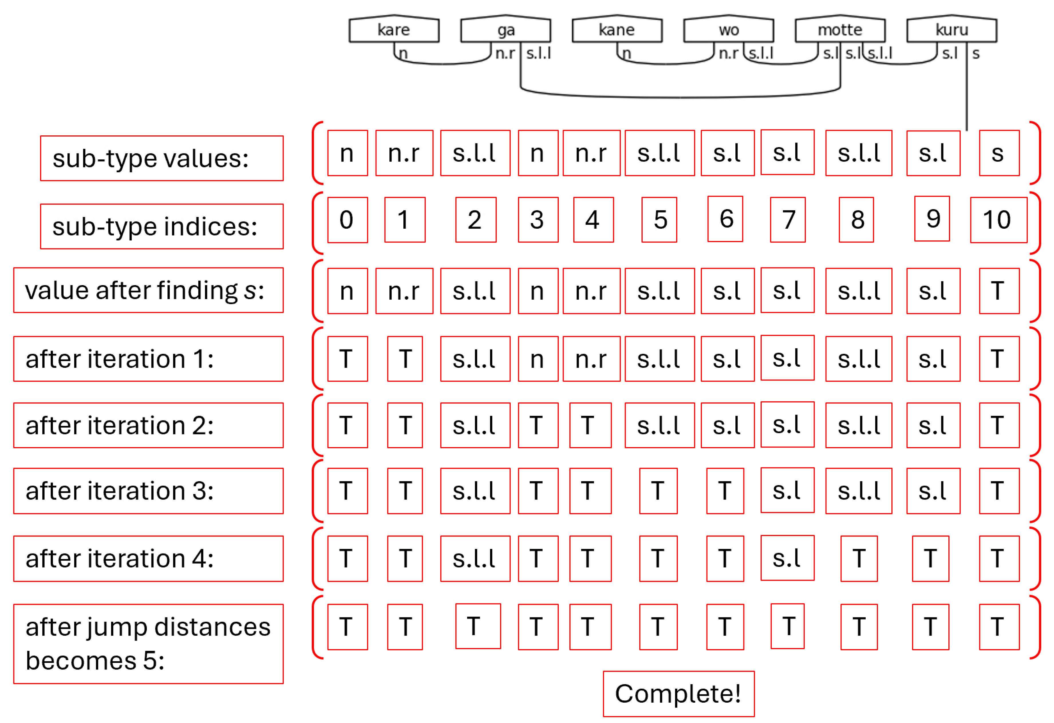
In the latter case, the contents of the sub-types scratch list case, the scratch list is passed into python’s set function, which returns the unique items of the list as a new list. In other words, it removes duplicate entries. This new list is then passed into the len function, which counts how many items are in the set. When that count is one, this means that all the sub-types have been marked True—all sub-types are either s or paired with the appropriate adjoint. This means the processing is complete.
The actual creation of the morphisms is done in the inner for-loop. For each item in the sub-types scratch list, there are several potential values the sub-type could take. Each of these is checked in an if-elif construct. Each case is controlled by the current indexed item in the scratch list, which has a value that pairs with another sub-type from the left. These, then, are either left-adjoints that pair with the base type (i.e., h.l to h), base types that pair with right-adjoints (i.e., n to n.r), or double left-adjoints that pair with single left-adjoints (s.l.l to s.l). If one of these valid pairing situations is found between the index and the index summed with the current jump distance, then a match has been found and it is time to construct a morphism. This is done with another helper method as shown in Figure 53.
Figure 53.
Linking Sub-types with a Cup.
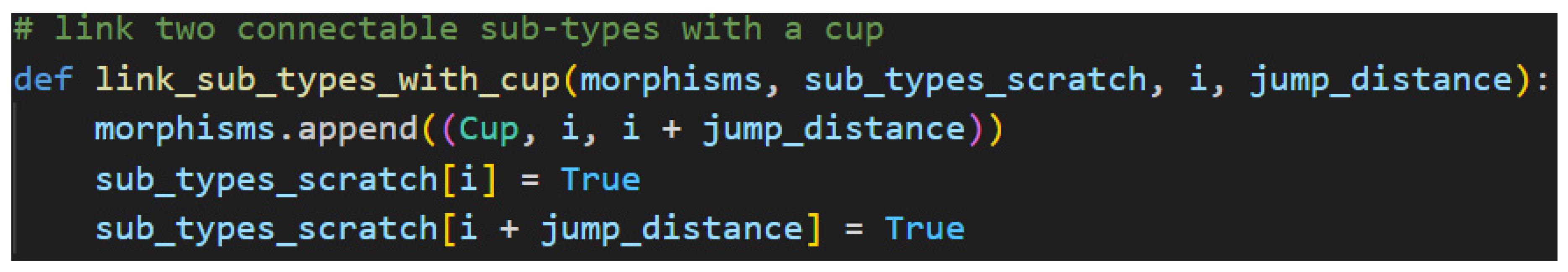
Figure 54.
Jump Distances Illustrated.
In Figure 53, a morphism is first created using lambeq’s Cups, the current index, and the sum of the index with the jump distance. This represents the sub-type found on the left-side of the sentence being linked to the compatible sub-type on the right-side. The newfound morphism is then appended to the morphism list, and the two linked sub-types are marked True because they are now paired. Further iterations of the loop will ignore them. The process continues until the sub-types are all linked, which means all the necessary morphisms have been created, in worst case O(n2) time.
Figure 55.
Sub-type Scratch Values While Passing Through the Loops of Step 7.
Step 8. Now that the Word list—the typed sentence—and the morphism list have been created and populated, all that remains is to draw the diagram. This is accomplished with a single line of code thanks to lambeq’s capabilities. That line is found in Figure 56.
The typed sentence—a list of lambeq Words—and the morphisms—a list of lambeq Cups—are provided to create pregroup diagram static method of the Diagram class. At this point, the algorithm has fully prepared Japanese text aligned with the grammar model to be passed to lambeq, which performs all the drawing logic from here.
2.7. Functors to Circuits
Now that pregroup diagrams can be constructed using the diagramizer algorithm, the next step is to functorially transform the pregroup diagrams into quantum circuits. This requires very little code at this point since lambeq provides all the core functionality. All that is needed is the pregroup diagram and an ansatz. Figure 57 contains the quantizer function.
While this function is short, there are a few important processes performed in Figure 57. First, there is the ansatz parameter. The argument passed in here could have many variations, but the specific definition of the ansatz is part of an experiment and should be handled in the main script instead of being rigidly defined in this function. An ansatz is a parameterized quantum circuit used as the starting point for solving a calculation (Wu et al., 2021). Like the initial parameters fed into a neural network, the starting point is updated, or tuned, as the circuit, or model, is trained.
Figure 58.
Defining an Ansatz in lambeq.

Next, the function’s body is discussed. The diagram argument is first normalized, meaning its morphisms—wires—are simplified into the most convenient and standardized diagrammatic representation via the snake equations (Quantinuum, 2024d; Coecke & Kissinger, 2017). After this form is achieved, the Cups are removed using lambeq’s RemoveCupsRewriter, which simplifies the diagram further. Removing the Cups reduces the post-selections in the quantum circuit, which yields significant performance improvements during Quantum Machine Learning (QML) experiment circuit evaluation (Quantinuum, 2024d; Aaronson, 2004). The simplified diagrams are then passed to the ansatz, which creates the quantum circuit from the diagram and returns it to the caller.
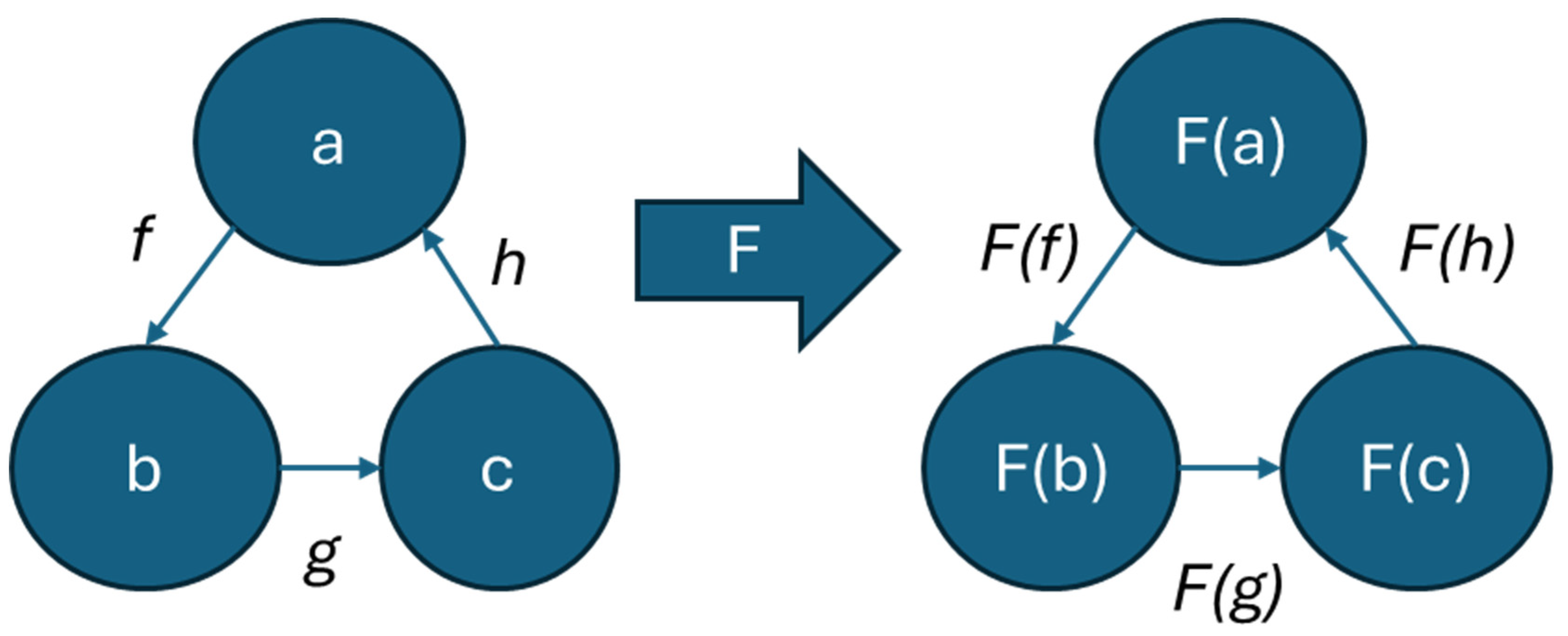
Transformation from diagram to circuit is made possible by the underlying mathematical structure that the two representations share. This transformation leverages a functor, a structure-preserving map in category theory that sends objects and morphisms of one category to another. In the case of the quantizer function shown in Figure 57, the functor is the ansatz, and it sends the structure of the string diagram to the structure of the quantum circuit. To put it simply, functors allow one to translate common structures between different mathematical contexts. They also, therefore, reveal common mathematical patterns in diverse disciplines.
Figure 59.
An Example Functor.
2.8. Reading the Circuits
Having gone through so much preprocessing to produce a quantum circuit containing the interpersonal metafunction of SFL, it is now time to examine and discuss the structure of an example circuit with some rigor. Figure 60 contains an instructive example as an exhaustive examination of the variety of possible circuits is far beyond the scope of the present investigation.
The precise structure of the quantum circuit is determined by the ansatz. Figure 60 was constructed using the ansatz defined in Figure 58, which accepts the three types—n, s, and h—used in the pregroup grammar, sets the number of processing layers, and the number of parameters—rotations—per single qubit as arguments. The types have been discussed at length, so nothing more will be said of them now. The ansatz in Figure 58 is the Instantaneous Quantum Polynomial (IQP) ansatz, which creates layers of Hadamard gates and Controlled Rotation about the z-axis (CRz) gates to implement diagonal unitary matrices. For each word represented with a single qubit, then, there are three phase rotations performed based on the n_single_qubit_params parameter. The angular value of a qubit, then, is set by Euler decomposition—three rotations about the coordinate axes.
Figure 60 is read from top-to-bottom as indicated by the open end of the 帰り[kaeri] wire; however, if one were to follow the sentences word order, then the diagram has a spiral structure, as indicated by the outermost arrows in Figure 61. Assuming one is reading left to right, the first word of the sentence appears in the second position. The flow then follows the CRz gates that join the first and second positions together. The first position then controls the third which, in turn, controls the fourth. The control qubit is marked by the solid black circle. If this qubit’s value is |1⟩, then the Rz operation is performed on the target qubit by some angle θ. That angle is represented in the diagram by the operations on the type of the word. The angle value, therefore, is parameterized as the value is not set when the circuit is defined. Ultimately, this allows for optimization and training of circuits.
The fourth position in the diagram represents ます[masu], which is represented by a single qubit. This is the h type of the sentence. This exercise, then, successfully encoded a Japanese grammar model with explicit honorifics into a quantum circuit. In this implementation, the h is controlled by a CRz gate and undergoes three phase rotations like the noun types do. It is left to further work whether h—the interpersonal metafunction—should be encoded the same way a noun is. For now, it is enough to have demonstrated that this encoding is possible but overlooked to the detriment of the field.
3. A Toy Experiment
To put these honorific circuits to the test, a toy experiment was devised. The goal of the experiment is to train a machine learning model to perform a binary classification task on a small, labeled dataset. The dataset consists of 260 Japanese sentences that are compatible with the grammar model defined and discussed above, which have been split into a training subset, validation subset, and test subset. Each sentence is labeled with a zero if it contains no honorifics or a one if at least one honorific type, h, is present. The model, then, will be learning to identify whether a sentence is polite or casual in Japanese. The experiment relies on the PennyLane model, which affords a hybridization of classical and quantum approaches (O’Riordan et al., 2020). PennyLane allows for training quantum circuits and neural networks simultaneously and the use of classical machine learning libraries, optimizers, and tools, providing the capability, for instance, to leverage transfer learning, or fine-tuning pre-trained classical models, with quantum circuits (Xanadu, 2024).
3.1. Materials & Methods
To begin, the experiment setup is briefly introduced. The variables under consideration here include choice of hyperparameters, ansatz, optimizer, loss and accuracy functions, trainer, and quantum backend. Figure 62 shows most of the variable assignments except for the trainer and backend, which are reserved for later.
The Figure 62 variables are discussed briefly in turn. The BATCH_SIZE refers to the number of diagrams to be simultaneously processed by the trainer. The EPOCHS are the number of complete passes to take over the training dataset. The learning_rate refers to the magnitude of adjustments to make to the model’s parameters. The trainer will use this value along with the optimizer to calculate the gradient and perform gradient descent based on the result, which should improve the model’s performance on subsequent epochs. Next, the SEED is used to set all the random number generators: one for PyTorch, one for the python random number generator, and one for numpy. The selected optimizer is AdamW, which is a standard in academia (Loshchilov & Hutter, 2019). The UnifyCodomainRewriter provides padding, so the underlying tensor shapes for all diagrams are the same. This is required for training with quantum circuits. The ansatz is the same as that in Figure 58 except it uses two layers of Hadamard gates and unitary matrices. Lastly, as a note, this experiment was not run on real hardware due to limited availability and time, though individual circuits were sent to IBM hardware and evaluated to demonstrate that these circuits are capable of running on real hardware. Training models on real hardware takes many hours or days due to queueing, so PennyLane’s default.qubit backend configuration was deemed suitable for the full experiment.
The selected evaluation function is accuracy, and the loss function is element-wise mean squared error (MSE). The evaluation function is used to provide a human-readable metric. The accuracy, then, refers to the number of correct predictions that the model made. The loss function is used, instead, during the training progress to adjust the magnitude and sign of parameter adjustments. It is useful for machine learning practitioners to see, but it means little to untrained eyes. These are defined in Figure 63.
The accuracy function calculates the ratio of correct predictions against total number of predictions. The y_hat variable is a tensor of predictions from the model. The y variable is the labels, or the known correct value. Whenever the y_hat variable is equivalent to the y variable, the model has predicted correctly. Behind this implementation, the values can be thought of as residing in a table. The rows in the table correspond between y_hat and y as the predictions or labels for a specific sentence. The max value in the row is the predicated binary classification—honorific or casual. The latter portion of the method takes the sum of the True predictions, converts this sum to a python number and devices that sum by the length of the y list. After this, the accuracy calculation is complete and is returned. The loss function calculation also takes y_hat—the predicted values—and y—the labels—as arguments. The function calls PyTorch’s neural network library’s native implementation of MSE. This loss function is a common standard, and because it is included with PyTorch, it is not discussed here in detail. Now, Figure 64 shows the trainer. All the variables and decisions made to this point in the experiment were made to support the instantiation of the PytorchTrainer and the training of the model.
3.2. Results
The results of the fifteen epochs are captured in Table 2 below. Figure 65, which follows, contains a graphical representation of the same data.
Table 2 contains results of the fifteen epochs of training based on the training subset and the validation subset of the data. The training set results, shown in columns two and four, exhibit strong positive trends. The loss maintains a trend of decreasing to under 2%, while the accuracy steadily increases to over 96%. This is the ideal behavior of training and is expected on the training set. This can yield, however, deceptive results, so models must always be checked against a validation set for a truer measure of performance. Columns three and five contain the results of the fifteen epochs against the validation set. The trend here is not so strong. In fifteen epochs, the validation set’s loss does not improve. It continues to hover between 20% and 30%. The accuracy, too, vacillates, eventually exceeding 61%. This reveals that the model is learning its training data very well; however, it may be learning it too well and overfitting.
The test subset is reserved for after the training completes and is used to gauge the performance of the model’s first prediction. Since the model has never seen the data in the test set before, it is considered a good test of the model’s would be performance in the wild. This is certainly a best practice and should confirm or refute the suspicion that the model needs fine-tuning. Upon performing its first prediction on the test set, the model’s accuracy was 70%, which confirms that the model is not ready for production, and it is back to the drawing board. That said, scores of 96%, 61% and 70% are better than guessing and an encouraging result. Since this experiment was only a toy to prove that interpersonal data from the Japanese language can be captured and encoded into quantum circuits using lambeq, it is deemed a success. A real-world experiment is left for future work.
Table 3.
Collected Results on Training, Validation, and Test Subsets as Percentages.
| Training Result | Validation Result | Test Result |
|---|---|---|
| 96.25% | 61.25% | 70.00% |
4. Conclusion: What it All Means
The present study has shown that encoding the interpersonal meaning of language into a quantum circuit is possible and could yield potentially fruitful results in QML experiments and quantum applications at large. Ultimately, this endeavor is an encouragement to the research community to open its eyes to new avenues of research, new realms of language beyond the strictly textual, and to consider the larger philosophical implications of what might be found in said realms. Language encompasses the full spectrum of human experience, so experiments should as well. Furthermore, it is up to researchers to examine beneath the unturned stones of non-English languages, hunting the pearls which may be found there hiding in plain sight. The fullness of human experience, thought, and expression cannot be contained within the single dimensional of textual meaning. Multi-dimensional considerations of language yield much fuller results and may, in fact, capture an image of the greater pattern beneath language and the universe itself (Wang-Máscianica et al., 2023; Waseem et al., 2022). The complexities of language are too great to view from only one angle. A fuller picture may reveal a pathway to the larger truth for which humankind has always searched.
4.1. Summary of Contributions
This work provides the following contributions to the wider QNLP community:
- 13.
- Extending lambeq’s type functionality to handle interpersonal types by defining the custom type h and testing this type with a toy experiment
- 14.
- Providing a Japanese grammar model, utilities, and a novel algorithm for parsing Japanese sentences using lambeq and making the source code available on GitHub for other researchers to use (Walton, 2024b)
- 15.
- Encourages the exploration of different language models, like SFL and considering non-textual information in further experiments
- 16.
- Introduces the concept of multi-dimensionality in the Japanese language where vertical meaning refers to interpersonal information—SFL’s interpersonal metafunction—encoded in grammar and horizontal meaning refers to textual information—SFL’s textual metafunction
4.2. Summary of Avenues for Further Research
This work recommends the following avenues of future research based on its contributions:
- 17.
- Extending lambeq itself with a standardized h type and the ability to parse Japanese sentences natively
- 18.
- Exploring complex Japanese types that account for the subtle, yet crucial, differences between particles—nominative, accusative, and genitive cases, etc. (Walton, 2023)
- 19.
- Modify source code to improve input validation, い[i]-adjective identification and parsing, and the diagramizer algorithm, and, further, to make the grammar model more robust, covering conjunctions, additional uses of の[no], and the like
- 20.
- Consider other languages and other linguistic realities that are being missed by the research community’s focus on the English language
- 21.
- Applying more mathematical rigor to the concept of multi-dimensional meaning, extending it to account for all metafunctions of SFL, and, perhaps, presenting it as a conceptual space
- 22.
- Currently, the h type is represented in quantum circuits using the same Euler decomposition as a noun, so it is left to future work to investigate whether h should be encoded in a unique way
- 23.
- Create a version of the diagramizer algorithm that processes kanji and kana
Author Contributions
All contributions to this work were made by the author, Ryder Dale Walton.
Funding
This research received no external funding.
Acknowledgments
Special thanks are offered to my wife, Lindsay, our beautiful children, our extended family, and all our friends and co-workers for all their support and prayers. Also, thanks to Dimitri Kartsaklis for providing a working code sample of the UnifyCodomainRewriter. Without his help, the experiment would have taken considerably more troubleshooting time. Lastly, thanks to Matthieu Pageau for the inspiration to integrate computer science with theology, philosophy, and metaphysics.
Conflicts of Interest
The authors declare no conflicts of interest.
References
- Aaronson, S. (2004). Quantum computing, postselection, and probabilistic polynomial-time.
- Abbaszade, M., Salari, V., Mousavi, S. S., Zomorodi, M., & Zhou, X. (2021). Application of quantum natural language processing for language translation. IEEE Access, 9, 130434–130448. [CrossRef]
- Abbaszade, M., Zomorodi, M., Salari, V., Kurian, P. (2023). Toward quantum machine translation of syntactically distinct languages. [CrossRef]
- Cardinal, K. (2002). An algebraic study of Japanese grammar [Master’s thesis, McGill University]. eScholarship@McGill. https://escholarship.mcgill.ca/concern/theses/m326m3733.
- Cardinal, K. (2007). A pregroup analysis of Japanese causatives. Pacific Asia Conference on Language, Information and Computation (pp. 96–104). https://aclanthology.org/Y07-1009.
- Cerban, M. (2009). The interpersonal metafunction of clauses: Polarity and modality. Proceedings of the International Conference Challenges in Languages, Literature and Arts at the Beginning of the 21st Century, Germanic Languages, 1. https://ssrn.com/abstract=2768579.
- Chang, D. T. (2023). Variational quantum classifiers for natural-language text. [CrossRef]
- Coecke, B. (2010). Quantum pictoralism. Contemporary Physics, 51, 59-83. [CrossRef]
- Coecke, B. (2016). From quantum foundations via natural language meaning to a theory of everything. [CrossRef]
- Coecke, B. (2020). The mathematics of text structure. [CrossRef]
- Coecke, B. (2021). Compositionality as we see it, everywhere around us. [CrossRef]
- Coecke, B., de Felice, G., Marsden, D., & Toumi, A. (2018). Towards compositional distribution discourse analysis. Electronic Proceedings in Theoretical Computer Science, 283, 1–12. [CrossRef]
- Coecke, B., de Felice, G., Meichanetzidis, K., & Toumi, A. (2020). Foundations for near-term quantum natural language processing. [CrossRef]
- Coecke, B., de Felice, G., Meichanetzidis, K., & Toumi, A. (2021). How to make qubits speak. [CrossRef]
- Coecke, B. & Gogioso, S. (2022). Quantum in Pictures. Your Print Solution.
- Coecke, B., & Kissinger, A. (2017). Picturing Quantum Processes: A First Course in Quantum Theory and Diagrammatic Reasoning. Cambridge: Cambridge University Press.
- Coecke, B., Lewis, M., & Marsden, D. (2018). Internal wiring of Cartesian verbs and prepositions. Electronic Proceedings in Theoretical Computer Science, 283, 75-88. [CrossRef]
- Coecke, B. & Paquette, E. O. (2009, October 12). Categories for the practising physicist. [CrossRef]
- Coecke, B., Sadrzadeh, M., & Clark, S. (2010). Mathematical foundations for a compositional distributional model of meaning. [CrossRef]
- Coecke, B. & Wang, V. (2021). Grammar equations. [CrossRef]
- de las Cuevas, G., Klingler, A., Lewis, M., & Netzer, T. (2020). Cats climb entails mammals move: Preserving hyponymy in compositional distributional semantics. [CrossRef]
- Duneau, T. (2021). Parsing conjunctions in DisCoCirc. In Proceedings of the 2021 Workshop on Semantic Spaces at the Intersection of NLP, Physics, and Cognitive Science (SemSpace) (pp. 66–75). Association for Computational Linguistics. https://aclanthology.org/2021.semspace-1.7.
- Dvorak, J. D., & Walton, R. D. (2014). Clause as Message: Theme, Topic, and Information Flow in Mark 2:2-12 and Jude. Biblical and Ancient Greek Linguistics, 3, 31–85. https://www.academia.edu/8695843/Clause_as_Message_Theme_Topic_and_Information_Flow_in_Mark_2_1_12_and_Jude?sm=b.
- de Felice, G. (2022, December 13). Categorical tools for natural language processing. [CrossRef]
- de Felice, G., Toumi, A., & Coecke, B. (2021). DisCoPy: Monoidal categories in Python. Electronic Proceedings in Theoretical Compute Science, 333, 183-197. [CrossRef]
- https://doi.org/10.4204/EPTCS.333.13. [CrossRef]
- Feynman, R. (1982). Simulating physics with computers. International Journal of Theoretical Physics, 21, 467-488. https://web.archive.org/web/20190824203534/https://people.eecs.berkeley.edu/~christos/classics/Feynman.pdf.
- García, D. P., Cruz-Benito, J., & García- Peñalvo, F. J. (2023). Systematic literature review: Quantum machine learning and its applications. [CrossRef]
- Hall, E. T. (1976). Beyond culture. Anchor Press.
- Kartsaklis, D., (2015). Compositional distributional semantics with compact closed categories and Frobenius algebras. [Doctoral dissertation, Oxford University]. [CrossRef]
- Kartsaklis, D., Fan, I., Yeung, R., Pearson, A., Lorenz, R., Toumi, A., de Felice, G., Meichanetzidis, K., Clark, S., & Coecke, B. (2021). lambeq: An efficient high-level python library for quantum NLP. https://arxiv.org/abs/2110.04236.
- Lambek, J (1997). Type grammar revisited. LACL ’97: Selected Papers from the Second International Conference on Logical Aspects of Computational Linguistics. (pp. 1–27). Springer-Verlag. [CrossRef]
- Leung, A. (2016, June 17). Field, tenor and mode – a literacy framework for all subjects. Retrieved 2024, April 24, from https://aliceleung.net/2016/06/17/field-tenor-and-mode-a-literacy-framework-for-all-subjects/.
- Lewis, M. (2019). Modeling hyponymy for DisCoCat. https://www.semanticscholar.org/paper/Modelling-hyponymy-for-DisCoCat-Lewis/56bfecd4061c069eaa3da4ec577da61155d512ce.
- Lewis, M. (2020). Towards logical negation in compositional distributional semantics. [CrossRef]
- Liu, J. (2023, September 19). Jonathan Liu – DisCoCirc. YouTube. Applied Category Theory. https://youtu.be/KoX8M4q-vdo?si=BXyVzdLqCnJR8I41.
- Liu, J. (2021). Language as Circuits. [Master’s thesis, Oxford University] https://www.cs.ox.ac.uk/people/bob.coecke/JonoThesis.
- Liu, J. Shaikh, R. A., Rodatz, B., Yeung, R. Coecke, B. (2023, November 29). A pipeline for discourse circuits from CCG. [CrossRef]
- Liu, M. & Kobayashi, I. (2022). Construction and validation of a Japanese honorific corpus based on Systemic Functional Linguistics. Proceedings of the 1st Workshop on Dataset Creation for Lower-Resourced Languages, 19-26. https://aclanthology.org/2022.dclrl-1.3/.
- Lorenz, R., Pearson, A., Meichanetzidis, K., Kartsaklis, D., & Coecke, B. (2021). QNLP in practice: Running compositional models of meaning on a quantum computer. [CrossRef]
- Loshchilov, I. & Hutter, F. (2019). Decoupled weight decay regularization. [CrossRef]
- Matthiessen, C. & Halliday, M. A. K. (1997). Systemic Functional Grammar: A first step into the theory. Retrieved 2024, April 24, from https://www.alvinleong.info/sfg/sfgintro.html.
- Meichanetzidis, K., Gogioso, S., de Felice, G., Chiappori, N., Toumi, A., & Coecke, B. (2021). Quantum natural language processing on near-term quantum computers. Electronic Proceedings in Theoretical Computer Science, 340, 213–229. [CrossRef]
- Meichanetzidis, K., Toumi, A., de Felice, G., Coecke, B. (2023). Grammar-aware sentence classification on quantum computers. Quantum Machine Intelligence, 5, 10. [CrossRef]
- Nieto, I. V. (2021). Towards Machine Translations with Quantum Computers. [Master’s Thesis, Stockholm University] diva. http://urn.kb.se/resolve?urn=urn:nbn:se:su:diva-196602.
- O’Riordan, L., Doyle, M., Baruffa, F., & Kannan, V. (2020). A hybrid classical-quantum workflow for natural language processing. Machine Learning: Science and Technology, 2(1). [CrossRef]
- Pizziconi, B. (2011). Honorifics: The cultural specificity of a universal mechanism in Japanese. In S. Mills & D. Z. Kádár (Eds.), Politeness in East Asia (pp. 45-70). Cambridge University Press. https://eprints.soas.ac.uk/7279/1/honorifics_the_cultural_specificity_of_a_universal_mechanism_in_japanese.pdf.
- Potts, C., & Kawahara, S. (2004). Japanese Honorifics as Emotive Definite Descriptions. Semantics and Linguistic Theory, 14, 253-270. https://www.semanticscholar.org/paper/Japanese-Honorifics-as-Emotive-Definite-Potts-Kawahara/6a863bfccdd563fc565d0f50773fd6976da3a8f6?utm_source=direct_link.
- Putz, V. & Svozil K. (2015). Quantum music. Soft Computing, NN, 1-5. [CrossRef]
- Quantinuum. (2024a). BobcatParser. lambeq. https://cqcl.github.io/lambeq/root-api.html#lambeq.BobcatParser.
- Quantinuum. (2024b). lambeq: An efficient high-level Python library for quantum NLP [Software]. GitHub. https://github.com/CQCL/lambeq.
- Quantinuum. (2024c). depccg support. In lambeq installation. Retrieved 2024, April 23, from https://cqcl.github.io/lambeq/installation.html#depccg-support.
- Quantinuum. (2024d). Rewriting. In lambeq documentation. Retrieved 2024, April 24, from https://cqcl.github.io/lambeq/examples/rewrite.html.
- Rizzo, I. (2019). A tale of deals, no deals, and baked beans. https://www.cs.ox.ac.uk/people/bob.coecke/DMM_Rizzo.pdf.
- Rodatz, B., Shaikh, R., & Yeh, L. (2021). Conversational negation using worldly context in compositional distributional semantics. [CrossRef]
- Sekizawa, R. & Yanaka, H. (2023). Analyzing syntactic generalization capacity of pre-trained language models on Japanese honorific conversion. [CrossRef]
- Shaikh, R., Yeh, Y., Rodatz, B., & Coecke, B. (2022). Composing conversational negation. Electronic Proceedings in Theoretical Computer Science 372, 352-367. [CrossRef]
- Takekuro, M. (2005). Attunement in interaction: Sequential use of Japanese honorifics. [Doctoral dissertation, University of California, Berkeley] eScholarship. https://escholarship.org/uc/item/1tr3s67n.
- Thompson, G., Bowcher, W. L., Fontaine, L., & Schönthal, D. (Eds.). (2019). The Cambridge Handbook of Systemic Functional Linguistics. Cambridge: Cambridge University Press.
- Toumi, A. (2022). “Category theory for quantum natural language processing.” https://arxiv.org/abs/2212.06615.
- van de Wetering, J. (2020). “ZX-calculus for the working quantum computer scientist.” . [CrossRef]
- Walton, R. D. (2023, May). Self-move and Other-move: Quantum Categorical Foundations of Japanese. Journal of Interdisciplinary Sciences, 7(1). https://journalofinterdisciplinarysciences.com/publication-archive/#1682826000846-990ae720-5e56.
- Walton, R. D. (2024a). “… God Said”: Toward a Quantum Theology of Creation. Open Theology, 10(1), 20220244. [CrossRef]
- Walton, R. D. (2024b). verticle_meaning [Software]. GitHub. https://github.com/Slidejiveman/verticle_meaning.
- Wang-Máscianica, V. & Coecke, B. (2021, September 16). Talking space: Inference from spatial linguistic meanings. [CrossRef]
- Wang-Máscianica, V., Liu, J., & Coecke, B. (2023, January 26). Distilling text into circuits. [CrossRef]
- Waseem, M. H., Liu, J., Wang-Máscianica, V., Coecke, B. (2022). Language-independence of DisCoCirc’s text circuits: English and Urdu. Electronic Proceedings in Theoretical Computer Science, 366, 50-60. [CrossRef]
- Wu, A., Gushu, Li., Wang, Y., Feng, B., Ding, Y., & Xie, Y. (2021). Towards efficient ansatz architecture for variational quantum algorithms. [CrossRef]
- Xanadu. (2024). PennyLane. Retrieved 2024, April 23, from https://pennylane.ai/.
- Xue, C., Chen, Z., Zhuang, X., Wang, Y., Sun., T., Wang, J., Liu, H., Wu, Y., Wang, Z., Guo, G. (2024). End-to-end quantum vision transformer: Towards practical quantum speedup in large-scale models. [CrossRef]
- Yeung, R. & Karsaklis, D. (2021). A CCG-based version of the DisCoCat framework. [CrossRef]
- Yoshikawa, M. (2023a). depccg: A Combinatory Categorial Grammar Parser [Software]. GitHub. https://github.com/masashi-y/depccg.
- Yoshikawa, M. (2023b). Issue #37: error while installing. depccg [Issue]. GitHub. https://github.com/masashi-y/depccg/issues/37.
- Zeng, W. & Coecke, B. (2016). Quantum algorithms for compositional natural language processing. Electronic Proceedings in Theoretical Computer Science, 221, 67–75. [CrossRef]
Figure 1.
SFL Diagram with Annotations to Emphasize the Interpersonal Metafunction. Note. The annotations are original to this paper. Current work in QNLP is focused on grammatical structures and textual meaning. The proposal here is to consider information between the red bars, especially tenor.
Figure 1.
SFL Diagram with Annotations to Emphasize the Interpersonal Metafunction. Note. The annotations are original to this paper. Current work in QNLP is focused on grammatical structures and textual meaning. The proposal here is to consider information between the red bars, especially tenor.
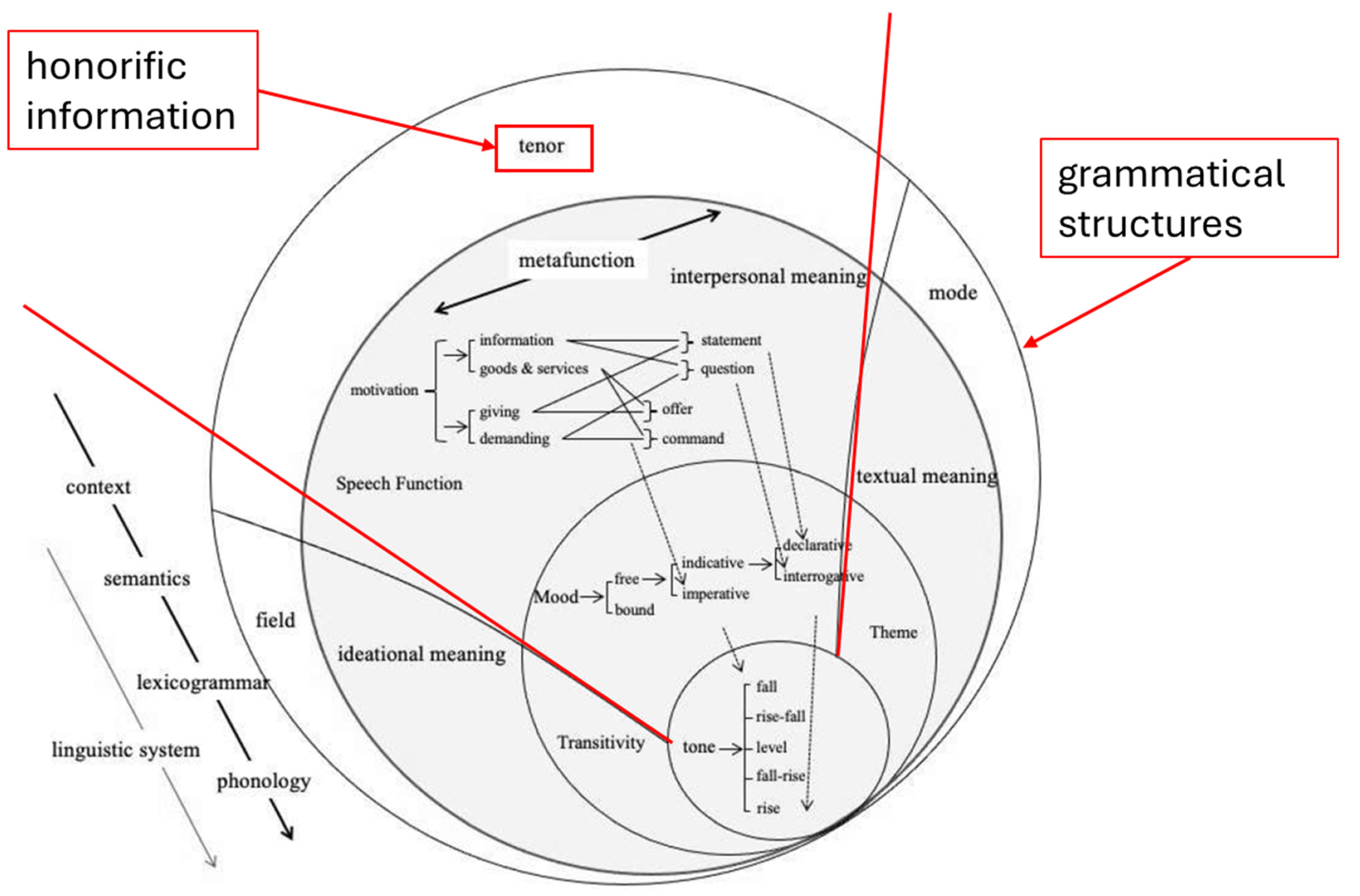
Figure 2.
The Vertical Dimension of Language.
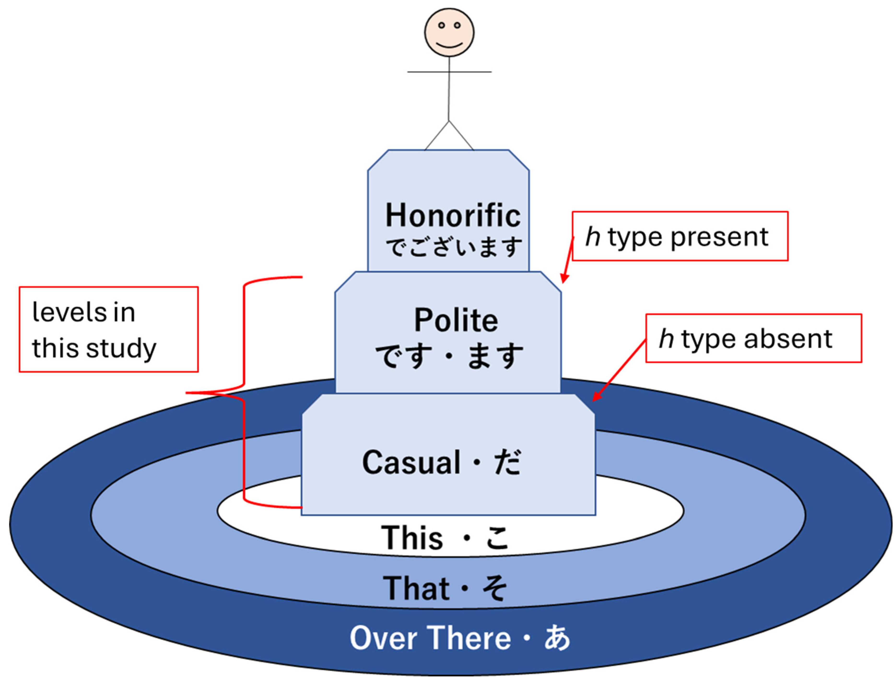
Figure 5.
Definition of Custom Honorific Types Alongside Standard Types in lambeq.
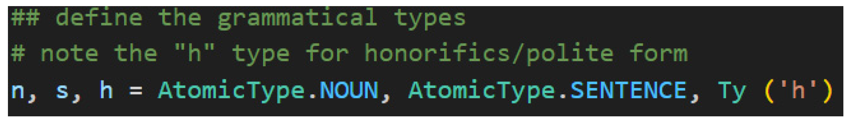
Figure 7.
Casual Predicate Complex Types.

Figure 13.
Polite Predicate Complex Types.

Figure 17.
Types for Names, Titles, and Pronouns.
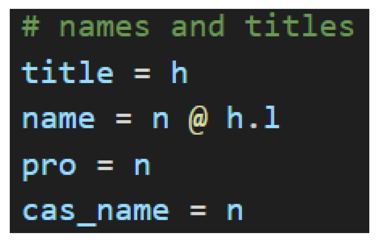
Figure 19.
Particles, Titles, and Sentence-enders as Special Words.
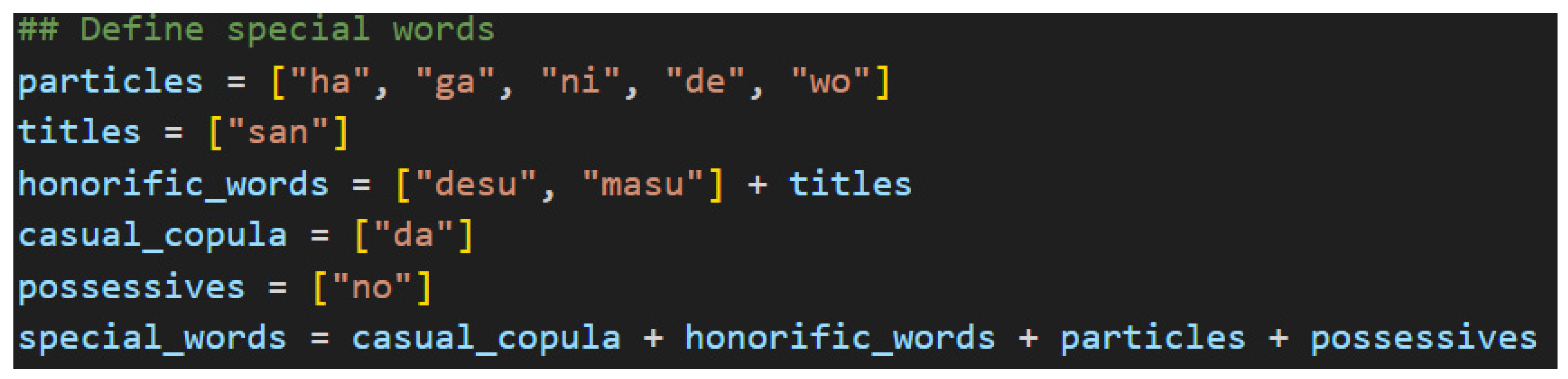
Figure 20.
Particle Type Assignments.
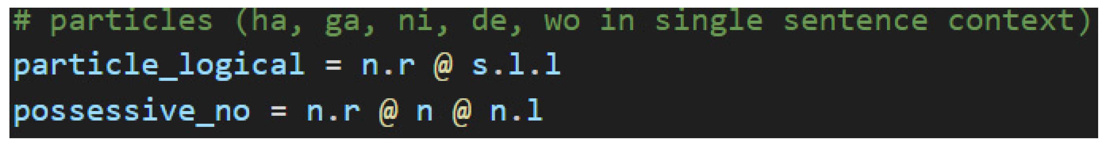
Figure 22.
Diagramizer’s Expected Token Format.
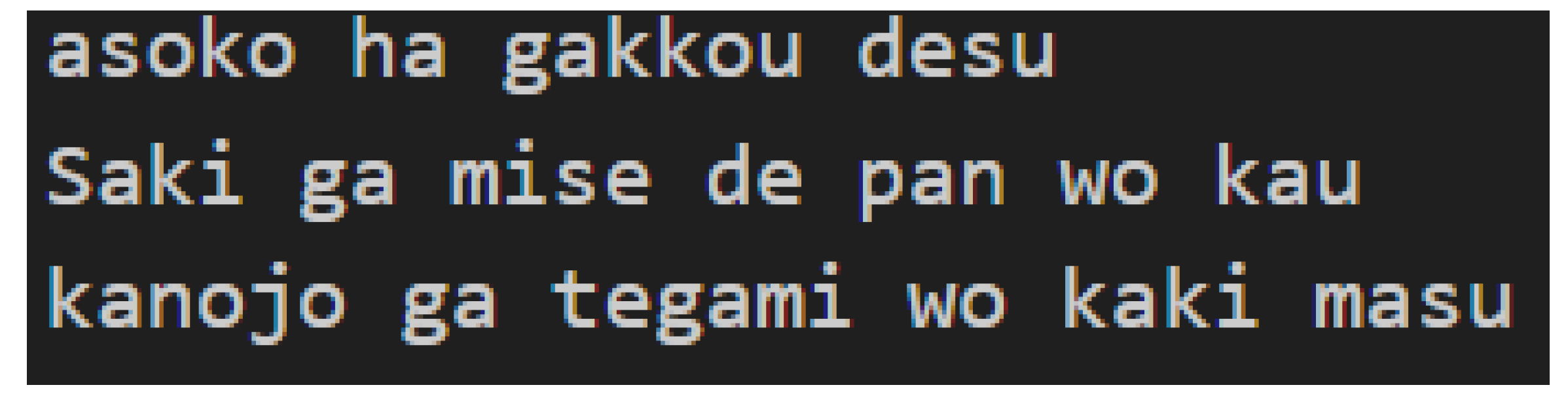
Figure 23.
The Diagramizer Algorithm.
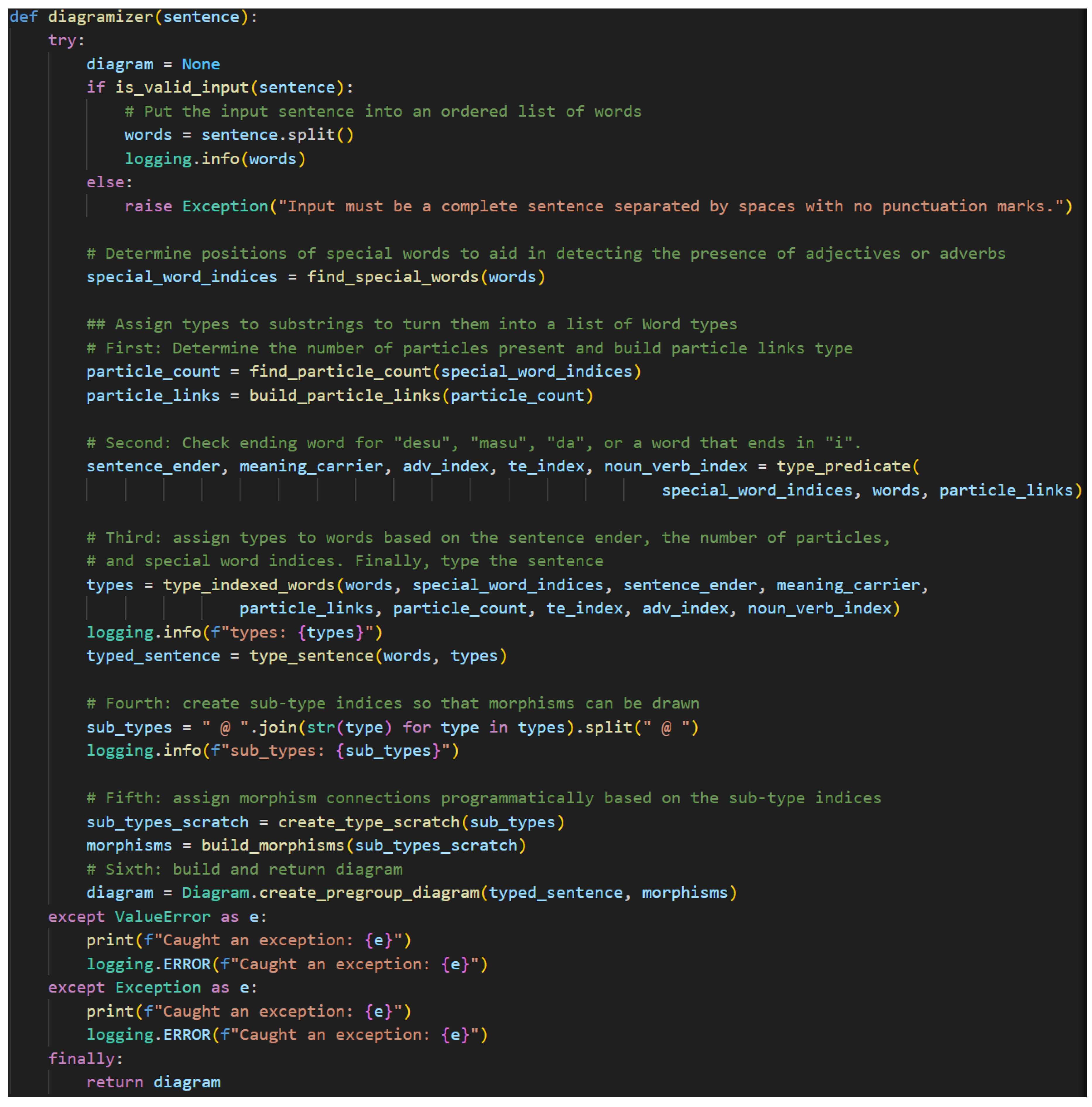
Figure 24.
Input Validation as Grammatical Validation.
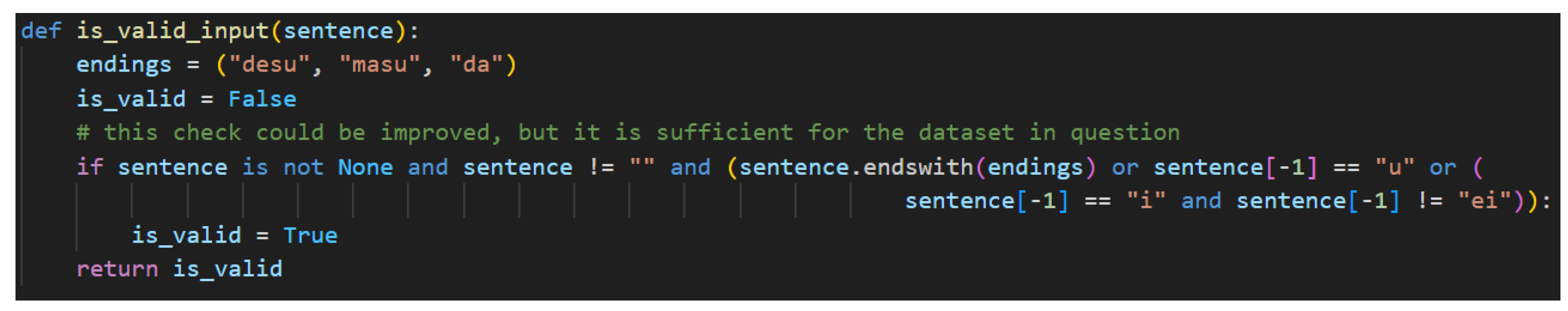
Figure 25.
Finding Special Word Indices.
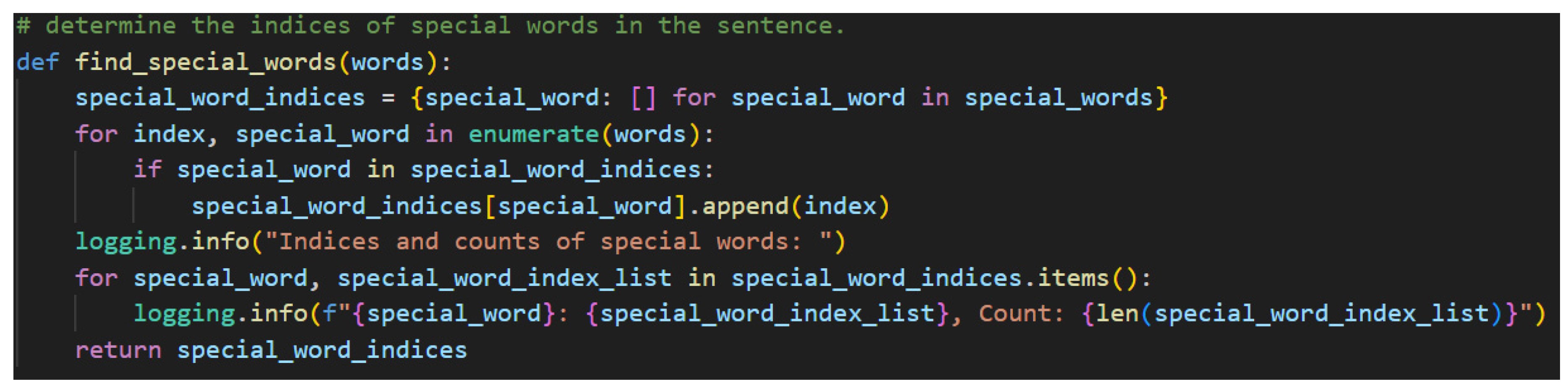
Figure 27.
Counting Particles.
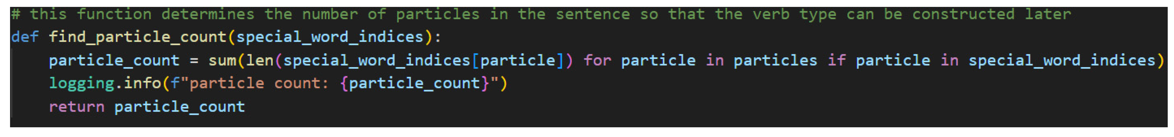
Figure 29.
Building the Particle Links.
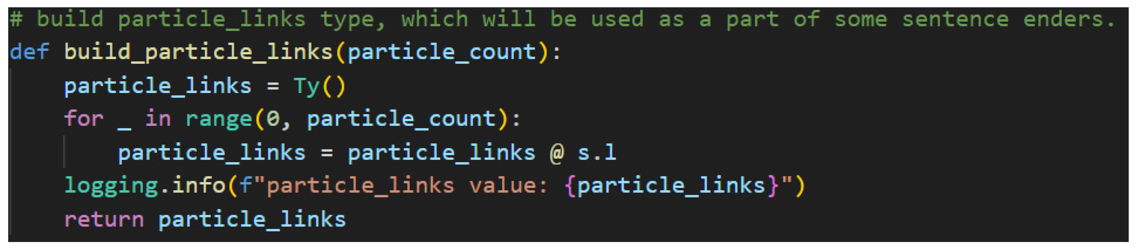
Figure 31.
Determining Which Sentence-ender is in the Predicate.
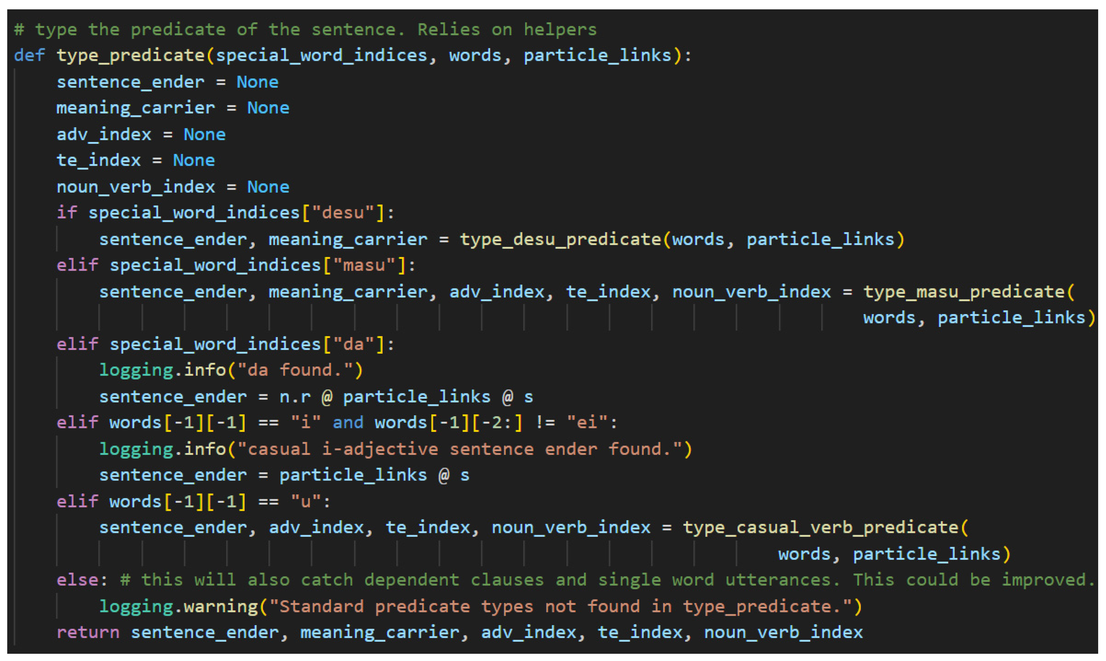
Figure 32.
Typing a です[desu] Predicate.
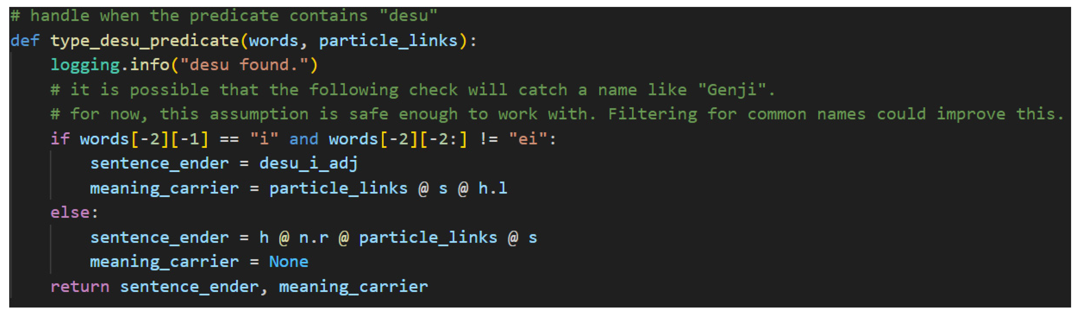
Figure 34.
Typing a ます[masu] Predicate.
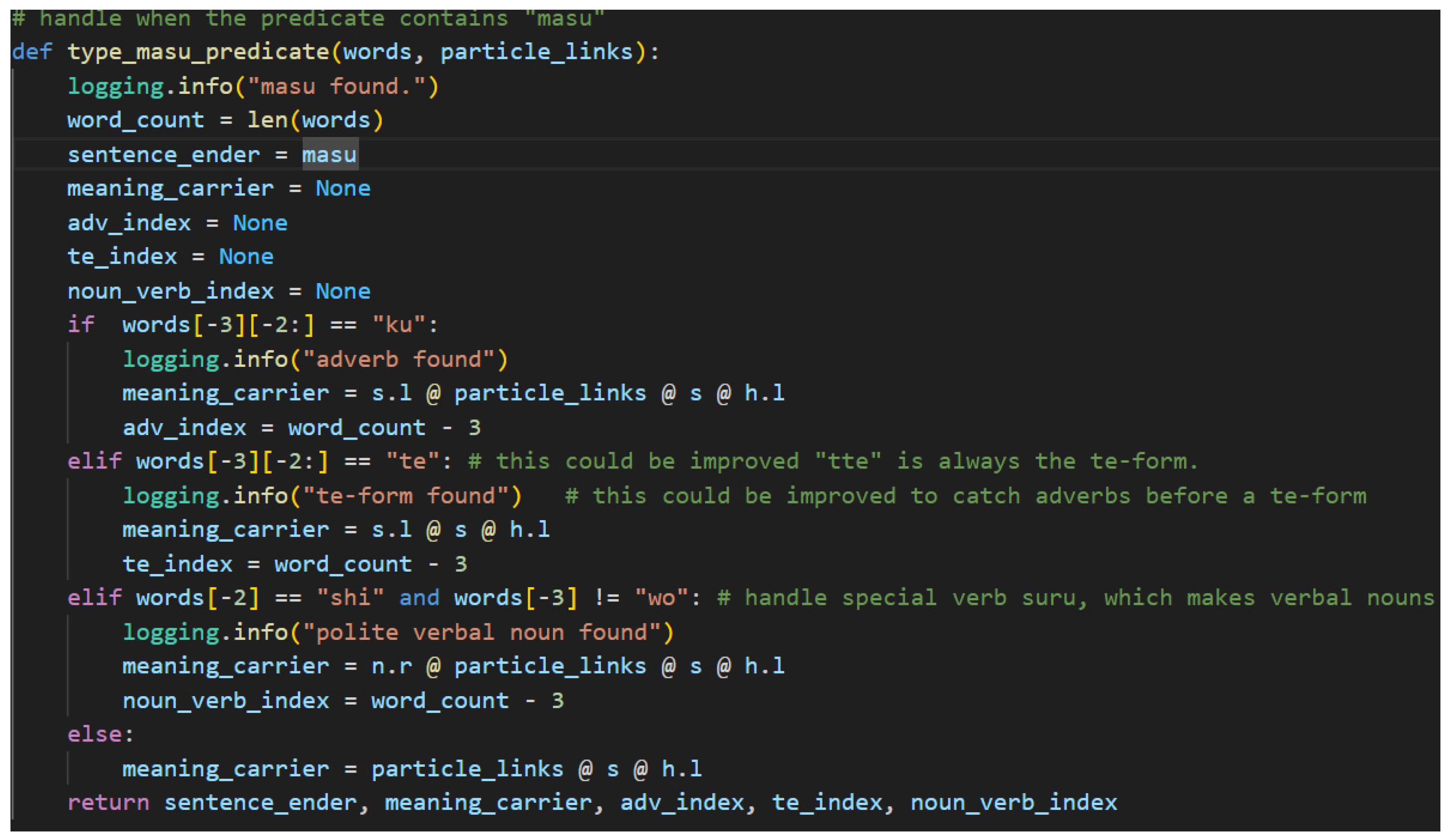
Figure 41.
Typing Indexed Words and Their Grammatically Related Words, Part One.
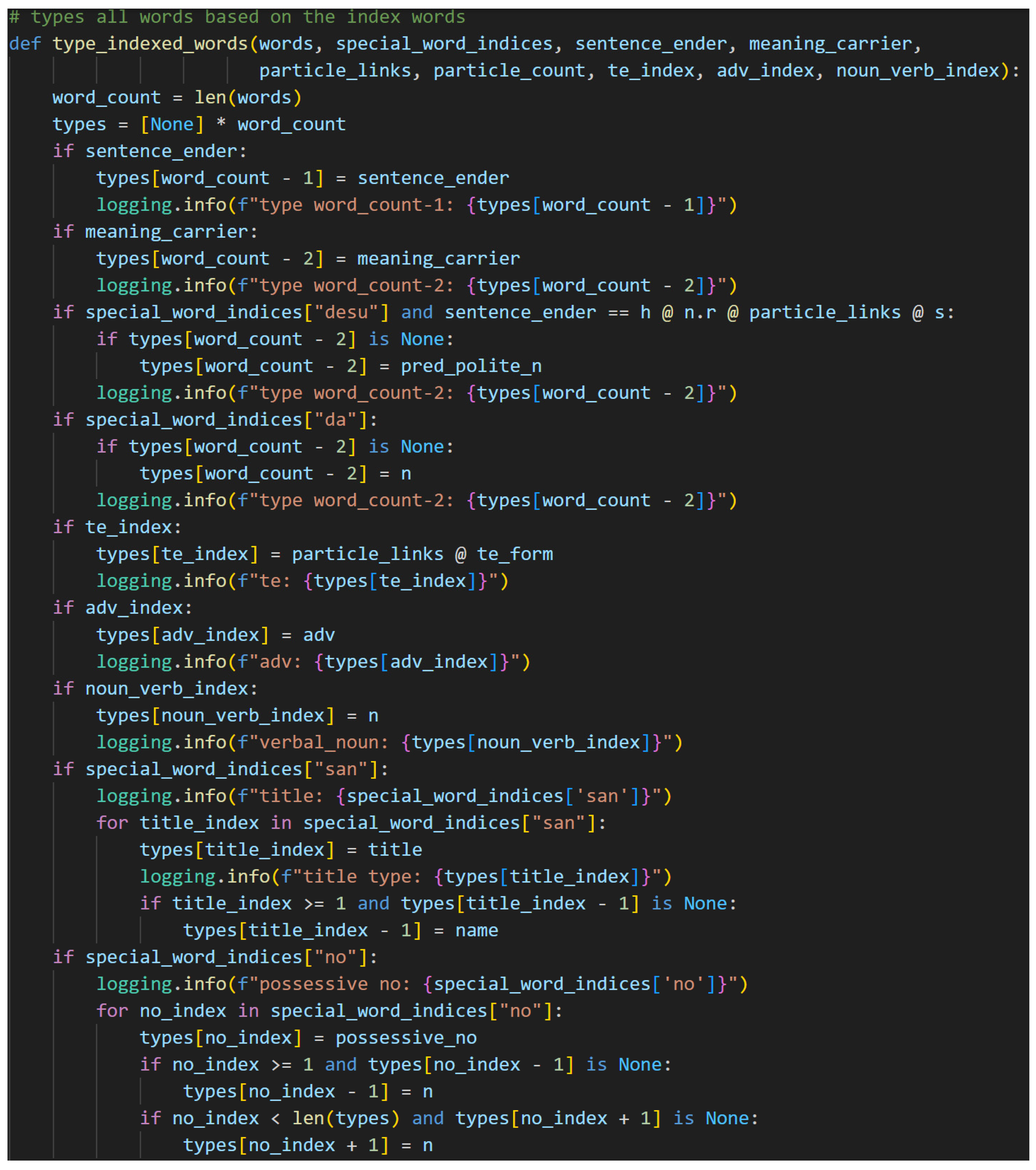
Figure 44.
Typing the Whole Sentence.
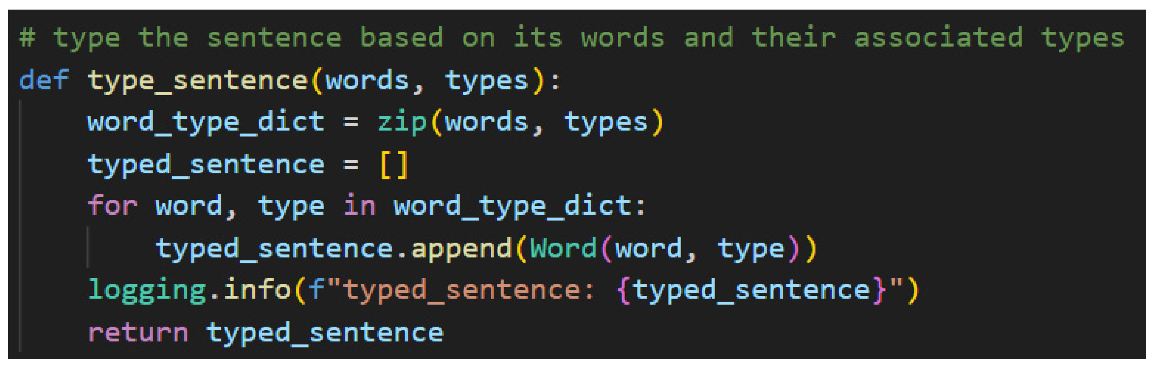
Figure 46.
Creating a List of Sub-types.

Figure 48.
Sub-type List Copying Function.
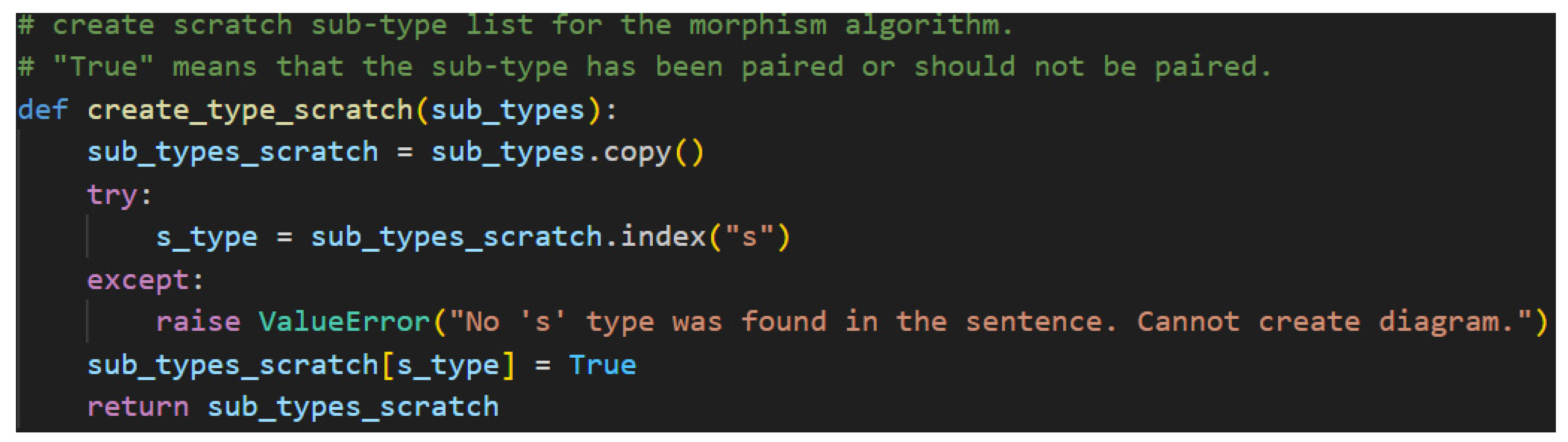
Figure 51.
Building Morphisms or Drawing Cups.
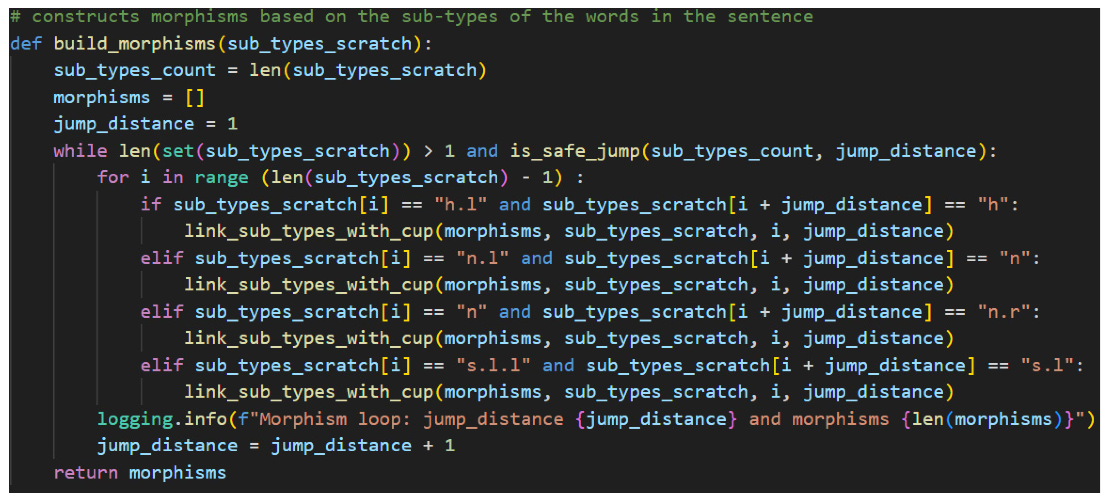
Figure 52.
Jump Distance Safety Function.
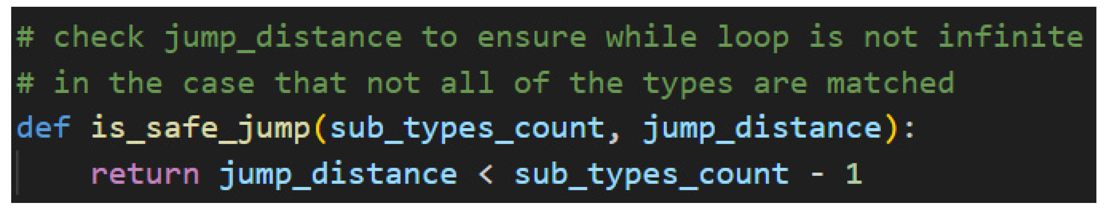
Figure 56.
Drawing a Diagram Using lambeq.

Figure 57.
Creating a Quantum Circuit from a Diagram.
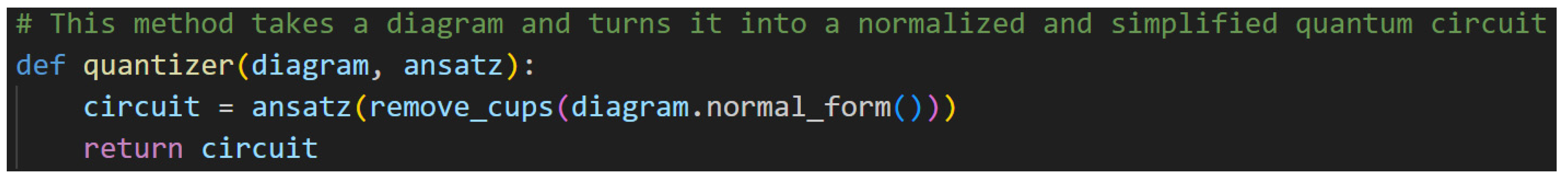
Figure 60.
A Quantum Circuit Encoded with Interpersonal Information.
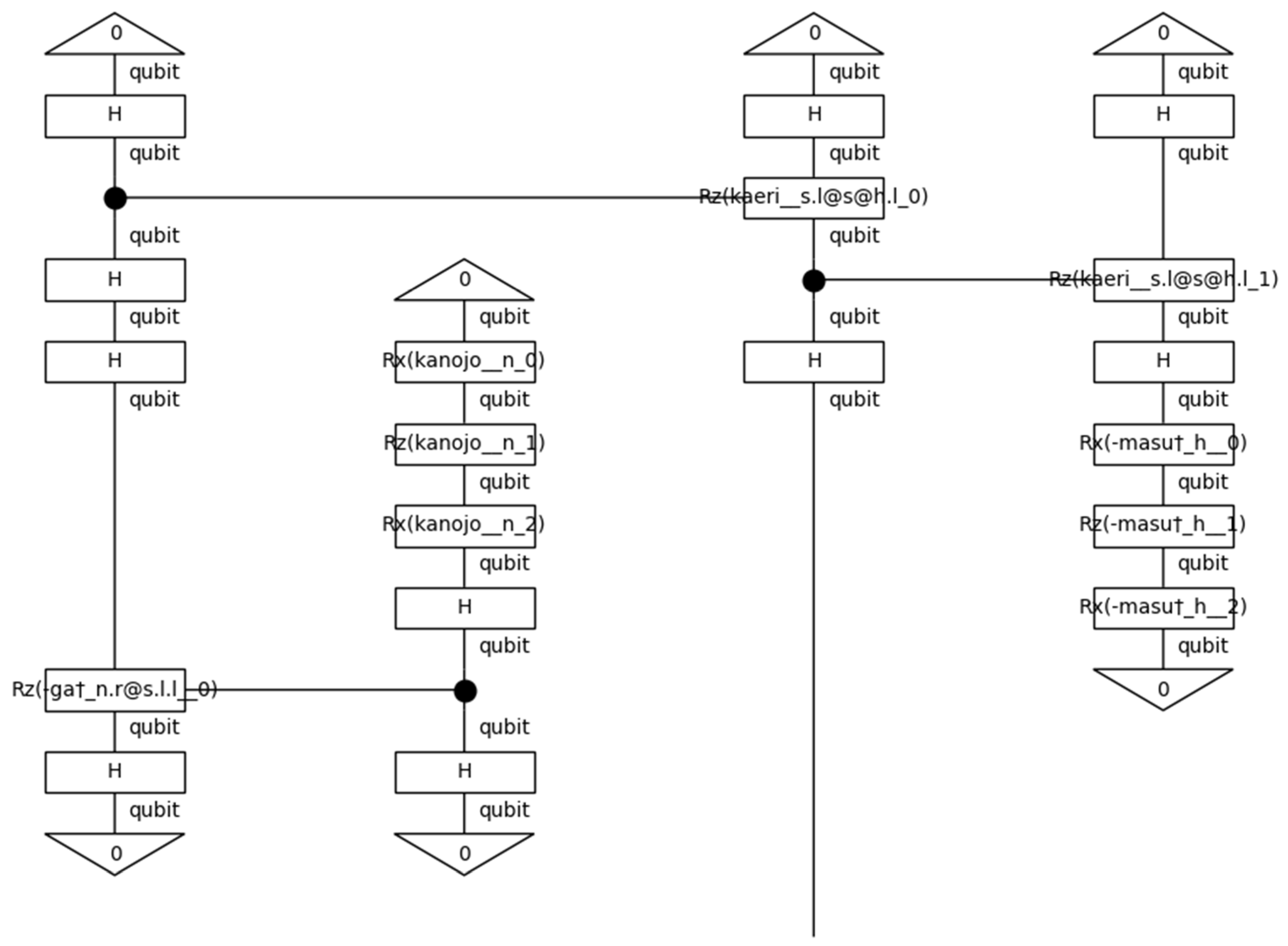
Figure 61.
Quantum Circuit Revisited and Labeled.
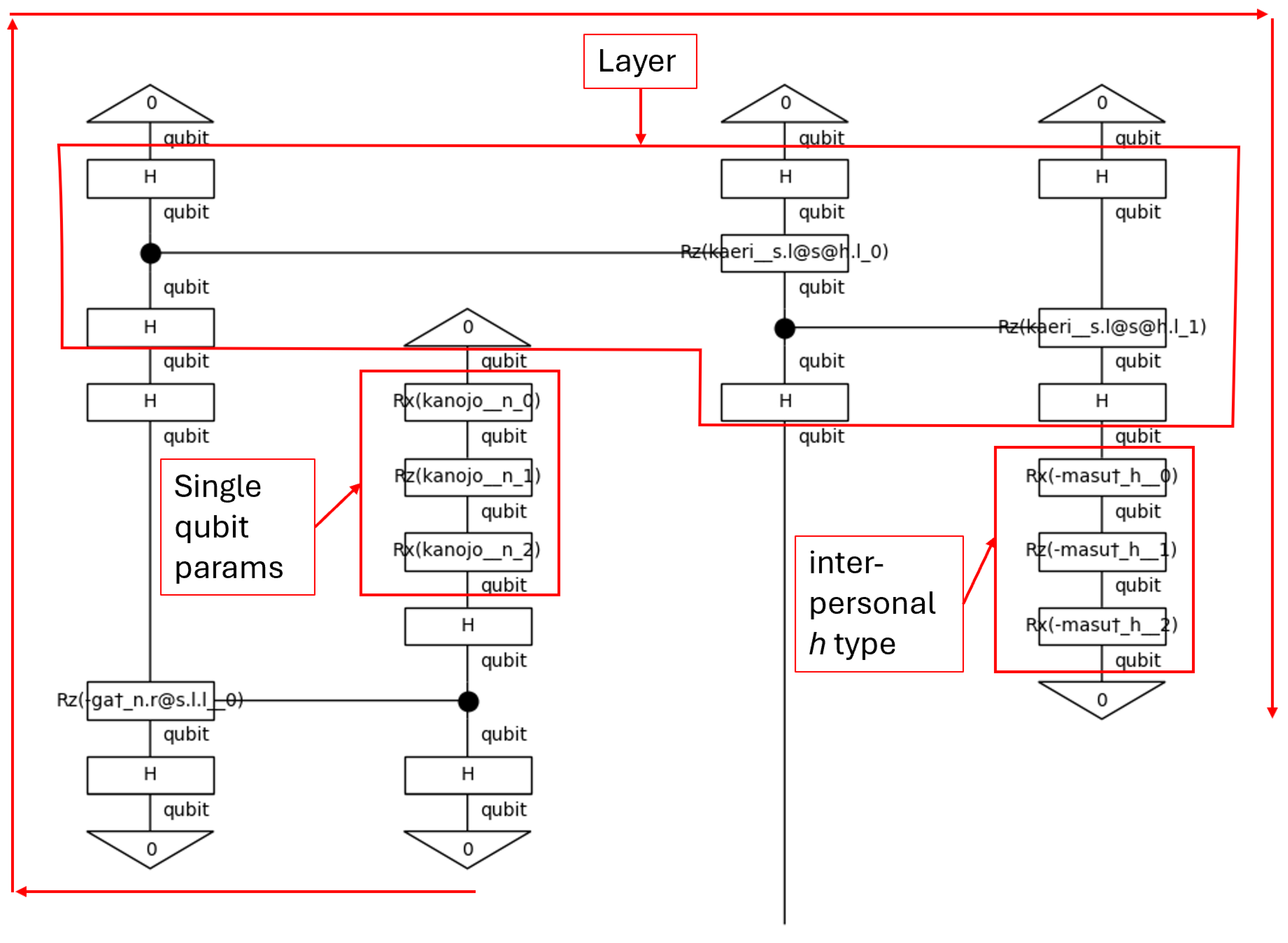
Figure 62.
Hyperparameters and Other Variables.
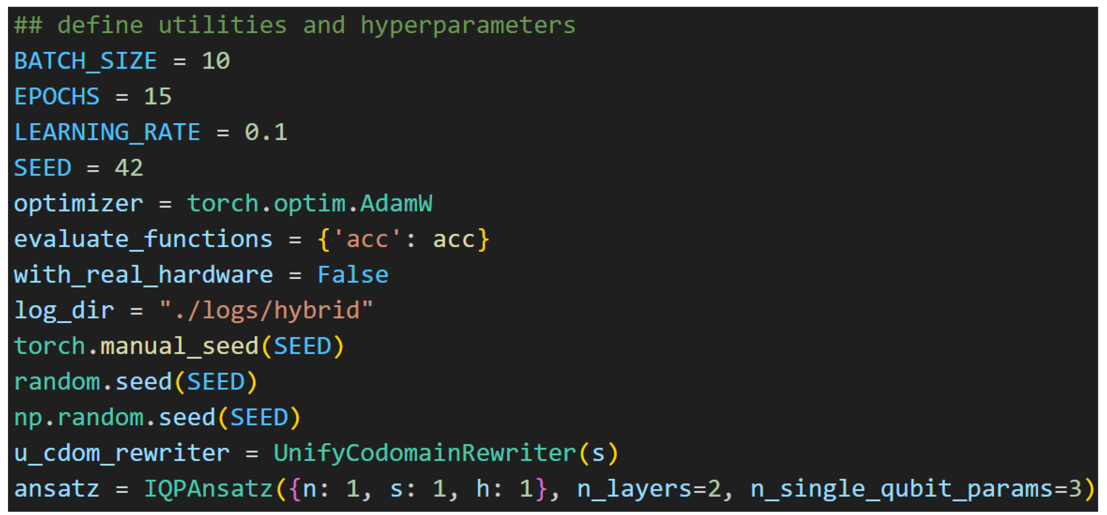
Figure 63.
Evaluation and Loss Functions.
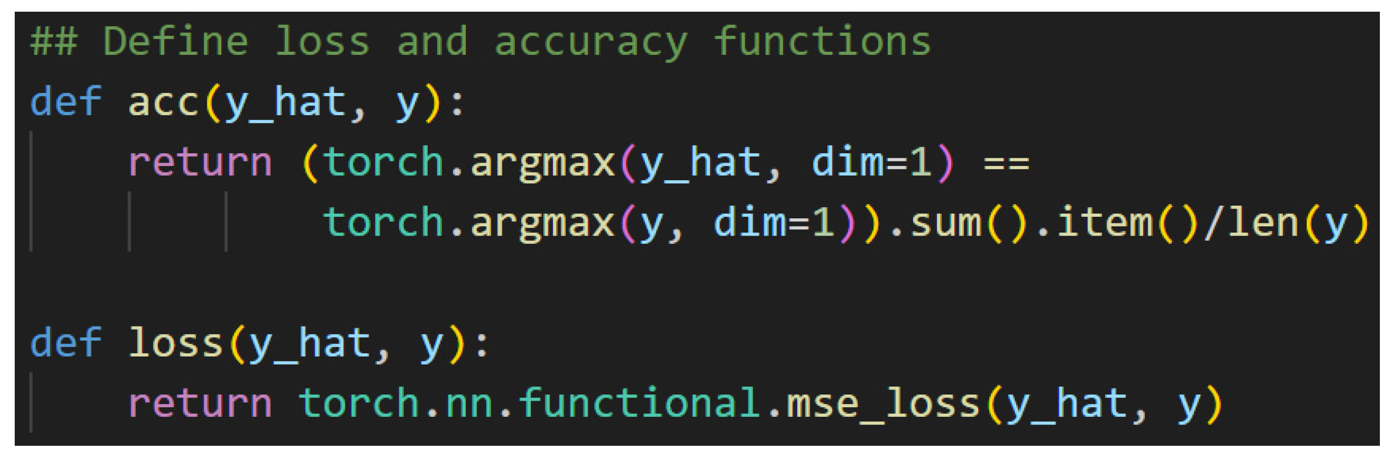
Figure 64.
Training an ML Model Using Pytorch and Quantum Circtuits.

Figure 65.
Graphical Representation of Table 2Note. For this experiment, early stopping, a feature that ends a model’s training early when it detects the loss is not improving after a chosen number of epochs, was not enabled. The diagram here shows where early stopping would have triggered had it been activated.
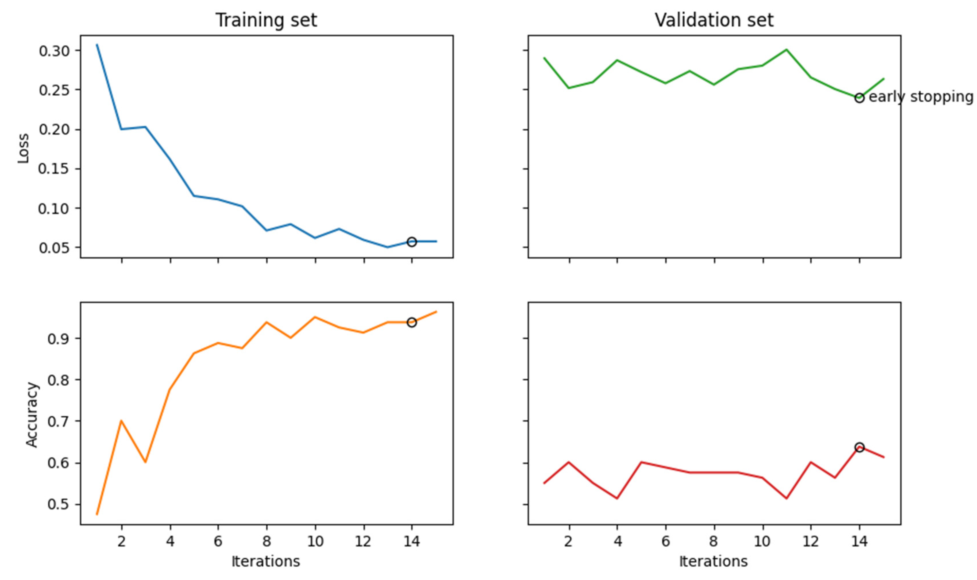
Table 2.
Results of Model Fitting to Training Set and Validation Set.
| Epoch | Training Set Loss | Validation Set Loss | Training Set Acc | Validation Set Acc |
|---|---|---|---|---|
| 1 | 0.3646 | 0.2893 | 0.4750 | 0.5500 |
| 2 | 0.2622 | 0.2516 | 0.7000 | 0.6000 |
| 3 | 0.2510 | 0.2591 | 0.6000 | 0.5500 |
| 4 | 0.1559 | 0.2869 | 0.7750 | 0.5125 |
| 5 | 0.1539 | 0.2719 | 0.8625 | 0.6000 |
| 6 | 0.0726 | 0.2577 | 0.8875 | 0.5875 |
| 7 | 0.0616 | 0.2731 | 0.8750 | 0.5750 |
| 8 | 0.0520 | 0.2560 | 0.9375 | 0.5750 |
| 9 | 0.0965 | 0.2755 | 0.9000 | 0.5750 |
| 10 | 0.0615 | 0.2800 | 0.9500 | 0.5625 |
| 11 | 0.0500 | 0.3003 | 0.9250 | 0.5125 |
| 12 | 0.0581 | 0.2650 | 0.9125 | 0.6000 |
| 13 | 0.0323 | 0.2503 | 0.9375 | 0.5625 |
| 14 | 0.0565 | 0.2390 | 0.9375 | 0.6375 |
| 15 | 0.0153 | 0.2631 | 0.9625 | 0.6125 |
Note. The accuracy values of columns four and five are reported as decimal values. Multiplying them by 100 will yield percentages.
Disclaimer/Publisher’s Note: The statements, opinions and data contained in all publications are solely those of the individual author(s) and contributor(s) and not of MDPI and/or the editor(s). MDPI and/or the editor(s) disclaim responsibility for any injury to people or property resulting from any ideas, methods, instructions or products referred to in the content. |
© 2024 by the authors. Licensee MDPI, Basel, Switzerland. This article is an open access article distributed under the terms and conditions of the Creative Commons Attribution (CC BY) license (http://creativecommons.org/licenses/by/4.0/).
Copyright: This open access article is published under a Creative Commons CC BY 4.0 license, which permit the free download, distribution, and reuse, provided that the author and preprint are cited in any reuse.


