Submitted:
27 April 2024
Posted:
29 April 2024
You are already at the latest version
Abstract
In this paper, we present a method for estimating GPS signals from visual information captured by a monocular camera mounted on a fixed-wing Unmanned Aerial Vehicle. The main challenge in visual odometry from aerial images is the computation of scale due to irregularities in the elevation of the terrain. That is, it is not possible to accurately convert from pixels in the image to meters in space, and the error accumulates. The contribution of this work is to reduce the accumulated error by comparing the images from the camera with satellite images. The algorithm has been tested in real-time experiments, and the results show that it is possible to eliminate the accumulated error using satellite images.
Keywords:
Unmanned Aerial Vehicle
; Geopositioning
; visual odometry
; Aerial Imagery
; feature extraction
1. Introduction
Unmanned Aerial Vehicles (UAV) were initially developed for military purposes [1]. The goal was to create realistic aircraft capable of reconnaissance missions for the U.S. Air Force. Now, drones have evolved into safe and cost-effective systems equipped with multiple sensors, finding extensive use in civilian, commercial, and scientific domains. They are utilized for applications such as aerial photography, infrastructure inspection, and search and rescue.
There are two types of motorized UAVs:
- Multirotor drones. These UAV are characterized by their design with multiple rotor blades. These drones are similar in concept to traditional helicopters but are typically smaller. The main distinguishing ability of rotary-wing drones is their ability to hover and take off and land vertically (VTOL).
- Fixed-wing. Similar to traditional airplanes. Unlike rotary-wing drones, they achieve lift through the aerodynamic forces generated by their wings as they move through the air.
Multirotor drones have some advantages over fixed-wing drones, such as the ability to hover, take off and land vertically, and change direction quickly. However, they also have some disadvantages, such as lower speed, shorter range, and higher energy consumption. This work focuses on fixed wing UAVs for which there are multiple classification tables based on size, weight, range, endurance, etc. The Table 1 shows a classification from [2]; The UAV used for image capture is categorized as small. Because of its range and operating altitude, this kind of UAV is suitable for reconnaissance, and monitoring.
To ensure safe takeoff, flight, and landing, these vehicles are equipped with multiple onboard sensors, such as GPS (Global Positioning System), environmental sensors (barometers and humidity sensors), and Inertial Navigation Systems (INS), which combine GPS data with INS data for accurate and reliable position information. In addition, depending on the task, imaging sensors (RGB or hyperspectral cameras), Light Detection and Ranging (LIDAR), air quality sensors, etc., may also be included.
The UAVs are piloted by a human on a Ground Control Station (GCS). The UAV is equipped with various actuators to control the surfaces of the aircraft (such as ailerons, elevators, and rudder), and an autopilot system which is responsible for stabilizing the aircraft, following pre-programmed flight paths, and responding to commands from the GCS.
The UAV communicates with the GCS. This communication is crucial for transmitting commands, receiving flight data, and sending back telemetry. The UAV continuously sends telemetry data to the GCS and it includes:
- Altitude, speed, and heading information.
- Battery status and remaining flight time.
- Sensor data such as temperature, humidity, or camera feed.
- GPS coordinates for position tracking.
From the GCS, it is possible to choose between different flight modes, such as:
- Manual
- Altitude hold
- Loiter mode
- Autonomous (pre-programmed missions)
2. Problem Statement
GPS signal is vital in order to achieve autonomy. Unfortunately, GPS signals can be intentionally blocked or disrupted in certain zones, including secure facilities, prisons, or sensitive government installations. There are multiple ways in which the GPS signal is intentionally restricted. For example, GPS jamming involves broadcasting radio signals on the same frequencies used by GPS satellites, overpowering the weaker GPS signals.
GPS spoofing is another way to restrict GPS. Here, a fake GPS signal that mimics legitimate signals is broadcast. GPS receivers are tricked into calculating incorrect position or velocity. Detecting GPS spoofing can be challenging, but several methods and technologies can help identify if a GPS signal is being spoofed [3,4,5,6,7,8,9,10].
Regardless of how the GPS signal is compromised, the mission may fail, since no other onboard sensor, like the Inertial Measurement Unit (IMU), is able to provide reliable position, velocity and altitude of the UAV since the state estimation drifts in time and becomes unusable after few seconds [11,12]. As a result, the UAV will take action depending on the flight mode or if the human pilot has visual contact with the vehicle, for instance, if there are no visual contact, most of the UAV have an automated routine to return to home, preventing it from completing its task. It is needed a solution where the UAV is able to keep flying or complete a mission even if the GPS signal is corrupted.
3. Related Work
There are multiple solutions for the GPS-denied problem, divided mainly into two approaches. The first approach is based on information from other agents, such as another vehicle [13,14,15], Unattended Ground Sensors (UGS) [16], or other types of packet transmission devices that serve as reference points for the UAV [17,18,19,20]. However, these techniques require the prior installation of these agents along the flight path, which can be unfeasible, especially if the agents are antennas that are difficult to transport or if passage to certain areas of the trajectory is restricted.
Not relying on other agents adds another level of autonomy to the system. Other approaches to addressing the GPS-denied problem are based on Visual Information. Some approaches use Simultaneous Localization And Mapping (SLAM), which is a technique used to locate the UAV in unknown environments [21,22,23]. However, depending on the altitude and the range, achieving visual SLAM techniques may not be feasible. Most of these works, however, are only reliable when the problem of localization is at low altitude and low range [11].
The main problem of using the previous approach for high-altitude UAVs (> 1000 m) is the estimation of the scale. That is, the transformation between pixel displacements and meters. Moreover, the nonlinear transformation between meters and latitude/longitude coordinates necessitates the prior setting of the Universal Transverse Mercator (UTM) zone. This scale could be computed based on IMU information and any other altitude sensor, such as LIDAR or barometer. However, the limitation of the LIDAR lies in its range, while the limitation of the barometer lies in its resolution.
When the UAV operates at high altitudes, LIDAR ceases to function, and we must rely on the barometer to calculate sea-level altitude. Then, with the help of an elevation map, we can calculate the difference between altitude above sea level and terrain elevation, thus determining a scale. However, limitations in barometer resolution result in errors when converting pixel displacement to meters, leading subsequent readings to start from an incorrect latitude/longitude coordinate, thereby resulting in a misreading of the elevation map. Without assistance or prior knowledge (landmarks) of the area we are flying in, errors will accumulate over time.
This paper is based on visual information and landmarks. In [11], the authors start from a previously created map. The helicopter flies over the area of interest to collect image data and construct a feature map for localization. The area is divided into a set of discrete regions (nodes), which are related to each other. The problem with this approach is that the UAV needs to previously fly over the area, and it would not be possible if the GPS signal is corrupted since the beginning of the flight.
Our work is more similar to [12]. Here, the authors start with geo-referenced satellite or aerial images, and then they search for landmarks. However, one disadvantage is that the range is limited, ensuring that the scale between pixels and meters remains constant. Even if we know the scale, it is impossible to guarantee that the elevation of the terrain remains constant in real reconnaissance or surveillance applications.
The contribution of this work is an algorithm that reduces the accumulated error in the estimation of the GPS signal based on aerial and satellite images for a UAV flying at over 1000 meters altitude above the terrain and a range of over 15 kilometers.
4. Methodology
The algorithm consists of two phases:
- Visual Odometry: At the moment of GPS loss, the algorithm estimates a latitude/longitude coordinate based only on monocular vision. The accumulated error in this phase will depend on the precision with which the scale is calculated.
- Reduction of accumulated error: We search for Correspondences between the UAV image and the georeferenced map to correct the estimation errors from the previous phase.
Assumption A1.
The aircraft is equipped with GPS signal from takeoff until some time after reaching the operating altitude.
Assumption A2.
We know the terrain elevation map
4.1. Visual Odometry
The experiments where performed on a small fixed-wing UAV flying with an altitude greater than 1000 meters. 700 Photos were taken on a path of approximately 18 km. Figure 1 shows the real path obtained from the GPS.
It is assumed the UAV enters into a GPS denied zone at the start of the path in Figure 1. When GPS is lost, the plane takes the first photo at (latitude, longitude) = (20.64226,-103.8181417). The path ends at (20.641845,-103.774705) and Figure 2 shows both images.
Figure 3 describes this stage of the algorithm. It starts when the UAV loses GPS signal, it begins to calculate the location estimation based on two consecutive images. First, features are extracted from both images using Oriented Fast and Rotated Brief (ORB).
Although ORB is one of the worst descriptors in terms of scale invariance, we can assume that the scale does not change substantially between both images, as the UAV will not change its altitude drastically during its operation. On the contrary, it is one of the algorithms that finds the largest number of keypoints and also one of the fastest. An analysis among different descriptor algorithms (ORB, BRISK, KAZE, AKAZE, SURF, and SIFT) can be found in [24]. The issue with detecting so many keypoints is the time it will take to establish correspondences between the images. To avoid processing all of them, we will only use matches with the shortest distance. This distance is a measure of the feature point similarity and we will denote with .
The first step is to consider the first two consecutive images and extract ORB features. We filter these matches to keep only the best ones. The best matches will be those whose similarity distance between features is less than a threshold. This threshold will depend on the images and the descriptor algorithm used. The heuristic used for this process is as follows: A test is conducted by plotting the best 200 matches, and the result is shown in the Figure 4.
Those matches were sorted based on similarity . This means that after 200 matches we have no matching error. The distance of similarity between features in the last match (the worst) in this experiment is 691. based on this information, we set a threshold of 300, trying to ensure that we only have good matches.
Once we know the correspondence between both point clouds, we compute the centroid of them
where is the centroid of the 2D points in the image i, x and y are the pixel coordinates of the feature j in image i and n is the number of good matches.
The idea is to estimate the UAV displacement from the displacement of one centroid to the next one. It is important to note that we have access to the angle of rotation since this is information obtained from the IMU and it is available even the GPS has been corrupted. Then, it reduces to calculating the UAV displacement in meters from the displacement of the centroids in pixel units.
There is an issue of ambiguity when trying to convert from pixels to meters. It may occur that a large displacement between the centroids is due to either moving very fast or having the keypoints very close to the UAV. Since altitude (estimated from the barometer) is another piece of information we have access to even without GPS, we use the barometer to heuristically scale s the altitude and use this value to convert from pixel units to meters. The scale s is calculated with
where s is the scale to transform from pixel to meters. is a constant heuristically selected and h represents the distance from the UAV to the ground, this is
where a is the UAV altitude and e the terrain elevation, taken from the digital elevation model (DEM) which is displayed in Figure 6.
Now it is needed to convert the last GPS signal from latitude/longitude to UTM coordinates. This is done using the open-source Geospatial Data Abstraction Library (GDAL). We start from the last coordinates obtained from GPS (before it has been denied) and convert them to UTM coordinates (Figure 7). In UTM system, the Earth is divided into 60 longitudinal zones, each spanning 6 degrees of longitude. These zones are numbered consecutively from west to east, starting at 180°W. Each zone is designated by a number from 1 to 60. Within each zone, a Transverse Mercator projection is used. This means that the surface of the earth is projected onto a cylinder that is tangent along a meridian within the zone.
UTM coordinates are typically referenced to a specific geodetic datum, such as WGS84 (World Geodetic System 1984), which provides a consistent reference surface for mapping. In the UTM system, locations on the Earth’s surface are specified using easting and northing coordinates, measured in meters. UTM provides relatively high accuracy for mapping and navigation within a specific zone. However, accuracy may decrease near the edges of zones due to distortion introduced by the projection. For a more detailed explanation about UTM coordinate system refer to [25,26,27].
The displacement of the UAV in meters is given by
where and represent the displacement in meters, is the displacement between the centroids in pixel units. is the yaw angle from the IMU and s the scale.
Once we have the last real latitude/longitude coordinates in UTM (meters), we can add the displacement of the centroids (in x and y direction), which has been already transformed into meters. Afterwards, the new UTM coordinate is converted back into latitude/longitude coordinates.
Up to this point, there are several issues involved. The first one is that the scale is calculated based on the altitude of the UAV relative to the terrain. Depending on the resolution of the elevation map and the resolution of the barometer, this scale may be computed incorrectly. If the scale is incorrect, then the conversion between pixels and meters will have an error, and the new coordinate will be calculated based on this incorrect scale.
The second problem is that this sequential algorithm relies on the previous location. If there was an error in the previous calculation, then we will be reading an incorrect elevation from the elevation map. If this reading is incorrect, then the scale for the next iteration will also have an error. In addition, if there are few keypoints, it is possible that we are computing the displacement based on some incorrect matches. In case the number of keypoints does not exceed a threshold, we will read the new yaw from the IMU, the distance between centroids that we had in the previous iteration (Figure 3).
As expected, there is no single optimal value for the constant that is suitable for all flight segments.
4.2. Reduction of Accumulated Error
So far, the presented algorithm is able to estimate the UAV location, but the prediction error accumulates over time. To address this issue, we introduce a novel algorithm based on satellite images (geo-referenced) and the flight plan.
Using satellite imaging for localization is not a new idea [29,30,31]. In [29], the authors presented a method to index ortho-map databases based on image features. This method allow high speed search of geo-referenced images. On the other hand, in [30] an extension of the Cross-View Matching Network (CVM-Net) for aerial imaging was presented. This paper offers a Markov localization framework that enforces temporal consistency. Finally, in [31] a localization method for a multi-rotor is discussed, where an Autoencoder is used to compress images to an embedding space, enabling the inner product kernel to compare images.
The above-mentioned projects can achieve high accuracy for their intended tasks, but they are not suitable for a tactical fixed-wing UAV which can navigate around 200 Km. In the presented case we have the following limitations:
- Power consumption of the Hardware: We are allow to supply small embedded hardwares like a Raspberry Pi 4 [32] or an Orange Pi 5 [33], to not compromise the entire system. This prevents us from using many of the techniques based on deep learning architectures.
- Onboard processing: Working in GPS-Denied zones commonly imply noisy or denied communication, requiring the UAV to compute GPS estimation onboard.
- Altitude estimation: low altitude Multi-rotors can achieved high precision due to laser or ultrasonic sensors, but for a tactical fixed-wing UAV we have to estimate altitude with a barometer sensor, that can have up to hundred meter of error.
- High range missions: Tactical UAV can reach up to 200 Km range of operation. Then the algorithm has to work with long paths.
To reduce the cumulative error in an efficient way we present the following pre-processing scheme (Figure 9), we detail this scheme in the following subsections:
4.2.1. Calculate Flight Plan
We provide the user two options: they can either upload a previous flight plan (a list of latitude-longitude coordinates), or we can calculate a Flight plan based on the elevation map, a starting point, an end point, and a working altitude. Firstly, we load the elevation map as an image and operate this image to calculate the safe zone based on the working altitude of the plane.
After, we use the Rapidly-exploring random trees (RRT*) [34] to calculate the safe coordinates in the map. RRT* is a random algorithm that generates random extensions from the start point. RRT* can be used in the non structure environments It can be applied in non-structured environments if we can calculate intersections between a known point and a newly generated point.
4.2.2. Filter Key-Points with the Flight Plan
Using a satellite image for reducing the accumulative error can be time-expensive, to avoid this, we apply a filter of key-points based on the flight plan. First we calculate the keypoints of a high-resolution image (this is very time-expensive but all this process is applied offline before the plane departs.
In contrast with the previous stage, where we used ORB, we are now implementing AKAZE [35] for feature extraction, which is an accelerated version of KAZE [36]. The reason for this choice is that AKAZE exhibits one of the best rotation invariance in contrast with other descriptors [24]. This is important because the UAV is not always heading north. The result of implementing AKAZE is shown in Figure 12.
The cardinality of key-points in Figure 12 (b) is 68061, this will imply a huge consumption of resources. To mitigate this, we filter these key-points by using the flight plan that we show in Figure 13 (a). In this case, the user provides a path instead of calculating it. Consider in Figure 14 (a), the histogram of the angular distance (in the latitude-longitude space) from each key-point to a point in the path (we use a linear interpolation of the path).
If we use a threshold of 0.005 over the distance to the path, we can obtain the filter key-points (Figure 13 (b)). In this case we count 25256 key-points, which is still a huge dataset to operate in real time. To have a better filter over the key-points we fit an exponential probability model, shown in (5), to the histogram of angular distance by using the maximum likelihood estimation (MLE) algorithm. In Figure 14 (b), we show the fitted exponential function.
We use the fitted exponential function to randomly sample key-points (without replacement), where key-points closer to the flight plan are more probable to be sample. This process has the virtue that can choose the cardinality of the filtered key-points and then bound the time needed for correction.
In Figure 15 (a), we illustrate a simulation of the probability distribution over the map. Notice that the probability of using a particular site depends on this probability function and the quantity of key-points. In Figure 15 (b), we present the final filtered key-points, limited to 5000. We find that this number of key-points allow us to achieve a real time application.
4.2.3. Spacial Indexing
Once we get the filtered points, we want to calculate efficiently the closest point to the current position of the plane. Comparing the current position of the UAV with each possible satellite key-point is an algorithm. This can be inefficient for real time applications.
the problem of rapidly find 2D or 3D points near a target point is known as spatial indexing [37]. This is a highly studied problem and there are some efficient solutions like K-dimensional tree (KD-tree) [38], Geohash [39], and Quad-tree [40]. In this paper, we implemented Quad-tree to get efficiently the K-nearest neighbors to search for a good match to reset position.
In Figure 16, we offer a general scheme for the Quad-tree algorithm. As its name suggest, Quad-tree is a tree data structure which each node has exactly four children. This allows to search points and query closest point in . The tree separates a two dimensional space in four parts, each par can subsequently be separated in other four parts.
We have validated that Quad-tree is enough to archive real time for our particular case, but we reserve a comparison with other spatial indexing techniques for a future research.
Finally, if we find a satellite keypoint in the current image, we use (6) to apply the coordinates correction with the offset between the keypoint in pixel coordinates and the center of the image (Figure 17). Then we transform this offset to a Latitude/Longitude offset with GDAL.
where and are the keypoint coordinates in the satellite image. x and y are the keypoint coordinates in the image. and are the image center. is the yaw orientation and is the rotation matrix, s the scale and is the transformation from UTM to Latitude/Longitude.
Figure 18 is utilized to provide a concise overview of this algorithm. There is a preprocessing step where we obtain keypoints from the satellite image. If, during the flight, we find one of these keypoints, we correct our geolocalization, otherwise, we estimate the coordinates with the visual odometry phase.
5. Results
Figure 19 shows the results of the correction algorithm. As can be seen, the error is not incremental in contrast with previous approach where only visual odometry was used.
Since the output is very noisy, it is decided to filter it with a Kalman Filter and the output is shown in Figure 20.
6. Conclusions
In this work, an algorithm that estimates the geolocation of a UAV in the absence of GPS signal was presented. Several factors impact this problem, such as the altitude of the UAV relative to the terrain, the geolocation where the experiment takes place, and the distance of the route. It was demonstrated that there is no way to optimize the scale for pixel-to-meter transformation, so the error will accumulate as the aircraft moves forward. The results show that it is feasible to use satellite image features to extract landmarks that help the UAV estimate its location, even though the images are not updated, have different intensity levels, and varying resolutions.
The algorithm filters the keypoints detected in the satellite image to ensure computational lightness and onboard execution capability to ensure autonomy.
It is demonstrated that this scheme prevents the error to increment over time even in long range missions.
Author Contributions
Conceptualization, J.G.-A. and C.V.; methodology, C.V.; software, J.G.-A., C.V. and P. I.-M.; validation, N. A.-D.; formal analysis, C.V. and N. A. -D; investigation, P. I.-M.; data curation, J. G.-A.; writing—original draft preparation, J. G.-A. and C.V.; writing—review and editing, N. A.-D.; visualization, P. I.-M.; supervision, J. G.-A.; project administration, J. G.-A. and C.V.; funding acquisition, N. A.-D. All authors have read and agreed to the published version of the manuscript.
Funding
This research was funded by University of Guadalajara through "Programa de Fortalecimiento de Institutos, Centros y Laboratorios de Investigación 2024".
Data Availability Statement
The data used to support the findings of this study are available from the corresponding author upon request. The data are not publicly available due to privacy.
Conflicts of Interest
The authors declare no conflicts of interest. The funders had no role in the design of the study; in the collection, analyses, or interpretation of data; in the writing of the manuscript; or in the decision to publish the results.
Abbreviations
The following abbreviations are used in this manuscript:
| DEM | Digital Elevation Model |
| GCS | Ground Control Station |
| GDAL | Geospatial Data Abstraction Library |
| GPS | Global Positioning System |
| HALE | High Altitude Long Endurance |
| IMU | Inertial Measurement Unit |
| INS | Inertial Navigation System |
| LIDAR | Light Detection And Ranging |
| MALE | Medium Altitude Long Endurance |
| ORB | Oriented Fast and Rotated Brief |
| UAV | Unmanned Aerial Vehicle |
| UGS | Unattended Ground Sensors |
| UTM | Universal Transverse Mercator |
| SLAM | Simultaneous Localization And Mapping |
| VTOL | Vertical Take Off and Landing |
References
- Gutiérrez, G.; Searcy, M.T. Introduction to the UAV special edition. The SAA Archaeological Record, Special Issue Drones in 356 Archaeology 2016, 16, 6–9. [Google Scholar]
- of Excellence, U.A.U.A.S.C. U.S. Army Unmanned Aircraft Systems Roadmap 2010-2035: Eyes of the Army; U.S. Army Unmanned Aircraft Systems Center of Excellence, 2010.
- Psiaki, M.L.; O’Hanlon, B.W.; Bhatti, J.A.; Shepard, D.P.; Humphreys, T.E. GPS spoofing detection via dual-receiver correlation of military signals. IEEE Transactions on Aerospace and Electronic Systems 2013, 49, 2250–2267. [Google Scholar] [CrossRef]
- Manfredini, E.G.; Akos, D.M.; Chen, Y.H.; Lo, S.; Walter, T.; Enge, P. Effective GPS spoofing detection utilizing metrics from commercial receivers. In Proceedings of the Proceedings of the 2018 International Technical Meeting of The Institute of Navigation, 2018.; pp. 672–689.
- O’Hanlon, B.W.; Psiaki, M.L.; Bhatti, J.A.; Shepard, D.P.; Humphreys, T.E. Real-time GPS spoofing detection via correlation of encrypted signals. Navigation 2013, 60, 267–278. [Google Scholar] [CrossRef]
- Khanafseh, S.; Roshan, N.; Langel, S.; Chan, F.C.; Joerger, M.; Pervan, B. GPS spoofing detection using RAIM with INS coupling. In Proceedings of the 2014 IEEE/ION Position, Location and Navigation Symposium-PLANS, 2014, 2014. IEEE; pp. 1232–1239. [Google Scholar]
- Jung, J.H.; Hong, M.Y.; Choi, H.; Yoon, J.W. An analysis of GPS spoofing attack and efficient approach to spoofing detection in PX4. IEEE Access 2024. [Google Scholar] [CrossRef]
- Fan, Z.; Tian, X.; Wei, S.; Shen, D.; Chen, G.; Pham, K.; Blasch, E. GASx: Explainable Artificial Intelligence For Detecting GPS Spoofing Attacks. In Proceedings of the Proceedings of the 2024 International Technical Meeting of The Institute of Navigation, 2024.; pp. 441–453.
- Chen, J.; Wang, X.; Fang, Z.; Jiang, C.; Gao, M.; Xu, Y. A Real-Time Spoofing Detection Method Using Three Low-Cost Antennas in Satellite Navigation. Electronics 2024, 13, 1134. [Google Scholar] [CrossRef]
- Bai, L.; Sun, C.; Dempster, A.G.; Zhao, H.; Feng, W. GNSS Spoofing Detection and Mitigation With a Single 5G Base Station Aiding. IEEE Transactions on Aerospace and Electronic Systems 2024. [Google Scholar] [CrossRef]
- Rady, S.; Kandil, A.; Badreddin, E. A hybrid localization approach for UAV in GPS denied areas. In Proceedings of the 2011 IEEE/SICE International Symposium on System Integration (SII). IEEE; 2011; pp. 1269–1274. [Google Scholar]
- Conte, G.; Doherty, P. An integrated UAV navigation system based on aerial image matching. In Proceedings of the 2008 IEEE Aerospace Conference. IEEE; 2008; pp. 1–10. [Google Scholar]
- Russell, J.S.; Ye, M.; Anderson, B.D.; Hmam, H.; Sarunic, P. Cooperative localization of a GPS-denied UAV using direction-of-arrival measurements. IEEE Transactions on Aerospace and Electronic Systems 2019, 56, 1966–1978. [Google Scholar] [CrossRef]
- Sharma, R.; Taylor, C. Cooperative navigation of MAVs in GPS denied areas. In Proceedings of the 2008 IEEE International Conference on Multisensor Fusion and Integration for Intelligent Systems. IEEE; 2008; pp. 481–486. [Google Scholar]
- Misra, S.; Chakraborty, A.; Sharma, R.; Brink, K. Cooperative simultaneous arrival of unmanned vehicles onto a moving target in gps-denied environment. In Proceedings of the 2018 IEEE Conference on Decision and Control (CDC). IEEE; 2018; pp. 5409–5414. [Google Scholar]
- Manyam, S.G.; Rathinam, S.; Darbha, S.; Casbeer, D.; Cao, Y.; Chandler, P. Gps denied uav routing with communication constraints. Journal of Intelligent & Robotic Systems 2016, 84, 691–703. [Google Scholar]
- Srisomboon, I.; Lee, S. Positioning and Navigation Approaches using Packet Loss-based Multilateration for UAVs in GPS-Denied Environments. IEEE Access 2024. [Google Scholar] [CrossRef]
- Griffin, B.; Fierro, R.; Palunko, I. An autonomous communications relay in GPS-denied environments via antenna diversity. The Journal of Defense Modeling and Simulation 2012, 9, 33–44. [Google Scholar] [CrossRef]
- Zahran, S.; Mostafa, M.; Masiero, A.; Moussa, A.; Vettore, A.; El-Sheimy, N. Micro-radar and UWB aided UAV navigation in GNSS denied environment. The International Archives of the Photogrammetry, Remote Sensing and Spatial Information Sciences 2018, 42, 469–476. [Google Scholar] [CrossRef]
- Asher, M.S.; Stafford, S.J.; Bamberger, R.J.; Rogers, A.Q.; Scheidt, D.; Chalmers, R. Radionavigation alternatives for US Army Ground Forces in GPS denied environments. In Proceedings of the Proc. of the 2011 International Technical Meeting of The Institute of Navigation. Citeseer, Vol. 508; 2011; p. 532. [Google Scholar]
- Trujillo, J.C.; Munguia, R.; Guerra, E.; Grau, A. Cooperative monocular-based SLAM for multi-UAV systems in GPS-denied environments. Sensors 2018, 18, 1351. [Google Scholar] [CrossRef] [PubMed]
- Radwan, A.; Tourani, A.; Bavle, H.; Voos, H.; Sanchez-Lopez, J.L. UAV-assisted Visual SLAM Generating Reconstructed 3D Scene Graphs in GPS-denied Environments. arXiv preprint arXiv:2402.07537, arXiv:2402.07537 2024.
- Kim, J.; Sukkarieh, S.; et al. 6DoF SLAM aided GNSS/INS navigation in GNSS denied and unknown environments. Positioning 2005, 1. [Google Scholar] [CrossRef]
- Tareen, S.A.K.; Saleem, Z. A comparative analysis of sift, surf, kaze, akaze, orb, and brisk. In Proceedings of the 2018 International conference on computing, mathematics and engineering technologies (iCoMET). IEEE; 2018; pp. 1–10. [Google Scholar]
- Fernández-Coppel, I.A. La Proyección UTM. Área de Ingeniería Cartográfica, Geodesia y Fotogrametría, Departamento de Ingeniería Agrícola y Forestal, Escuela Técnica Superior de Ingenierías Agrarias, Palencia, UNIVERSIDAD DE VALLADOLID 2001.
- Franco, A.R. Características de las coordenadas UTM y descripción de este tipo de coordenadas. Obtenido de http://www. elgps. com/documentos/utm/coordenadas_utm. h tml 1999.
- Langley, R.B. The UTM grid system. GPS world 1998, 9, 46–50. [Google Scholar]
- Dana, P.H. Coordinate systems overview. The Geographer’s Craft Project 1995.
- Wu, C.; Fraundorfer, F.; Frahm, J.M.; Snoeyink, J.; Pollefeys, M. Image localization in satellite imagery with feature-based indexing. In Proceedings of the XXIst ISPRS Congress: Technical Commission III. ISPRS, Vol. 37; 2008; pp. 197–202. [Google Scholar]
- Hu, S.; Lee, G.H. Image-based geo-localization using satellite imagery. International Journal of Computer Vision 2020, 128, 1205–1219. [Google Scholar] [CrossRef]
- Bianchi, M.; Barfoot, T.D. UAV localization using autoencoded satellite images. IEEE Robotics and Automation Letters 2021, 6, 1761–1768. [Google Scholar] [CrossRef]
- Gay, W. Raspberry Pi hardware reference; Apress, 2014.
- Noreen, I.; Khan, A.; Habib, Z. A comparison of RRT, RRT* and RRT*-smart path planning algorithms. International Journal of Computer Science and Network Security (IJCSNS) 2016, 16, 20. [Google Scholar]
- Alcantarilla, P.F.; Solutions, T. Fast explicit diffusion for accelerated features in nonlinear scale spaces. IEEE Trans. Patt. Anal. Mach. Intell 2011, 34, 1281–1298. [Google Scholar]
- Alcantarilla, P.F.; Bartoli, A.; Davison, A.J. KAZE features. In Proceedings of the Computer Vision–ECCV 2012: 12th European Conference on Computer Vision, Florence, Italy October7-13, 2012, Proceedings, Part VI 12. Springer, 2012; pp. 214–227.
- Begum, S.A.N.; Supreethi, K. A survey on spatial indexing. Journal of Web Development and Web Designing 2018, 3. [Google Scholar]
- Ram, P.; Sinha, K. Revisiting kd-tree for nearest neighbor search. In Proceedings of the Proceedings of the 25th acm sigkdd international conference on knowledge discovery & data mining, 2019, pp. 1378–1388.
- Huang, K.; Li, G.; Wang, J. Rapid retrieval strategy for massive remote sensing metadata based on GeoHash coding. Remote sensing letters 2018, 9, 1070–1078. [Google Scholar] [CrossRef]
- Tobler, W.; Chen, Z.t. A quadtree for global information storage. Geographical Analysis 1986, 18, 360–371. [Google Scholar] [CrossRef]
Figure 1.
Ground Truth. The path starts at the green marker and it ends at the red marker and measures approximately 18 km.
Figure 1.
Ground Truth. The path starts at the green marker and it ends at the red marker and measures approximately 18 km.
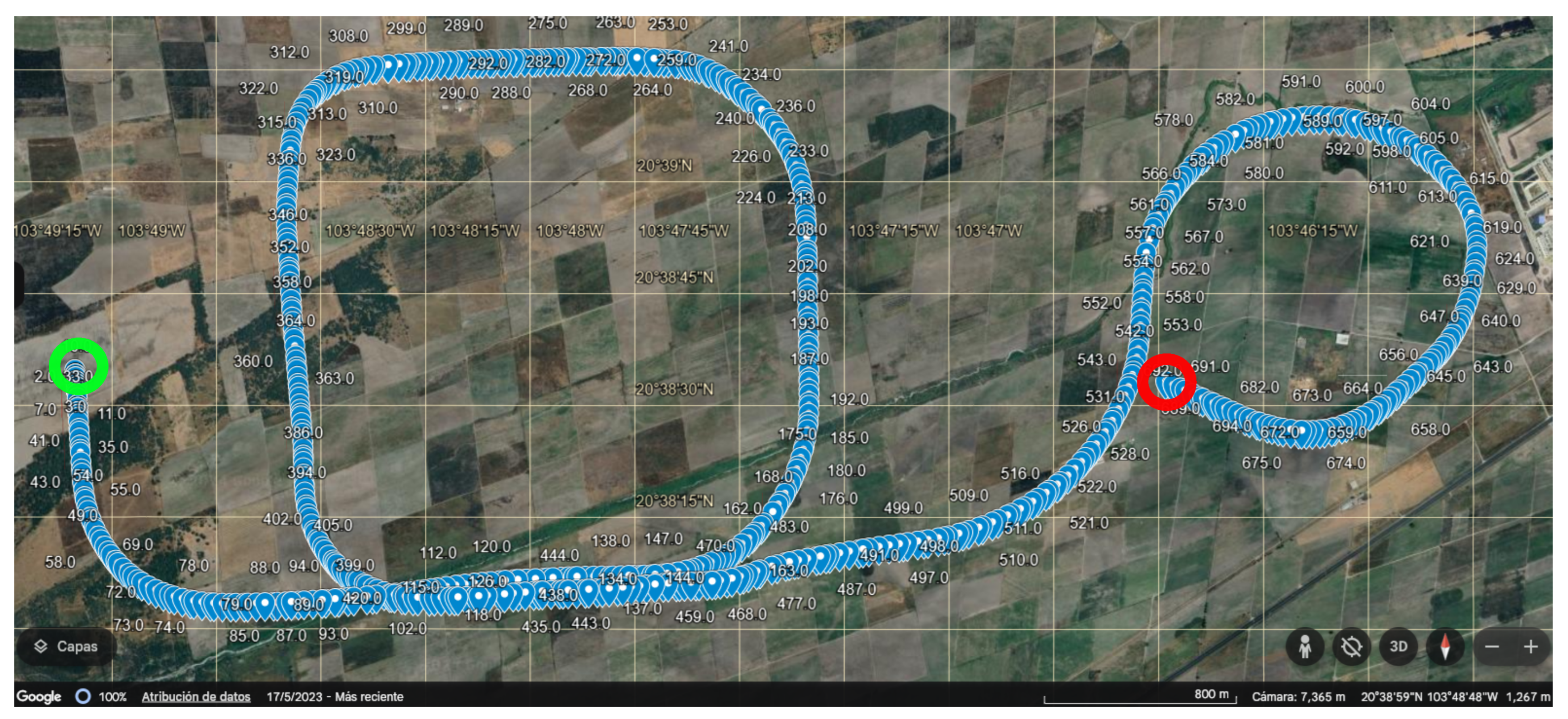
Figure 2.
First and final photo. It is assumed that GPS is lost at the first photo and it is not restored along the entire trajectory.
Figure 2.
First and final photo. It is assumed that GPS is lost at the first photo and it is not restored along the entire trajectory.
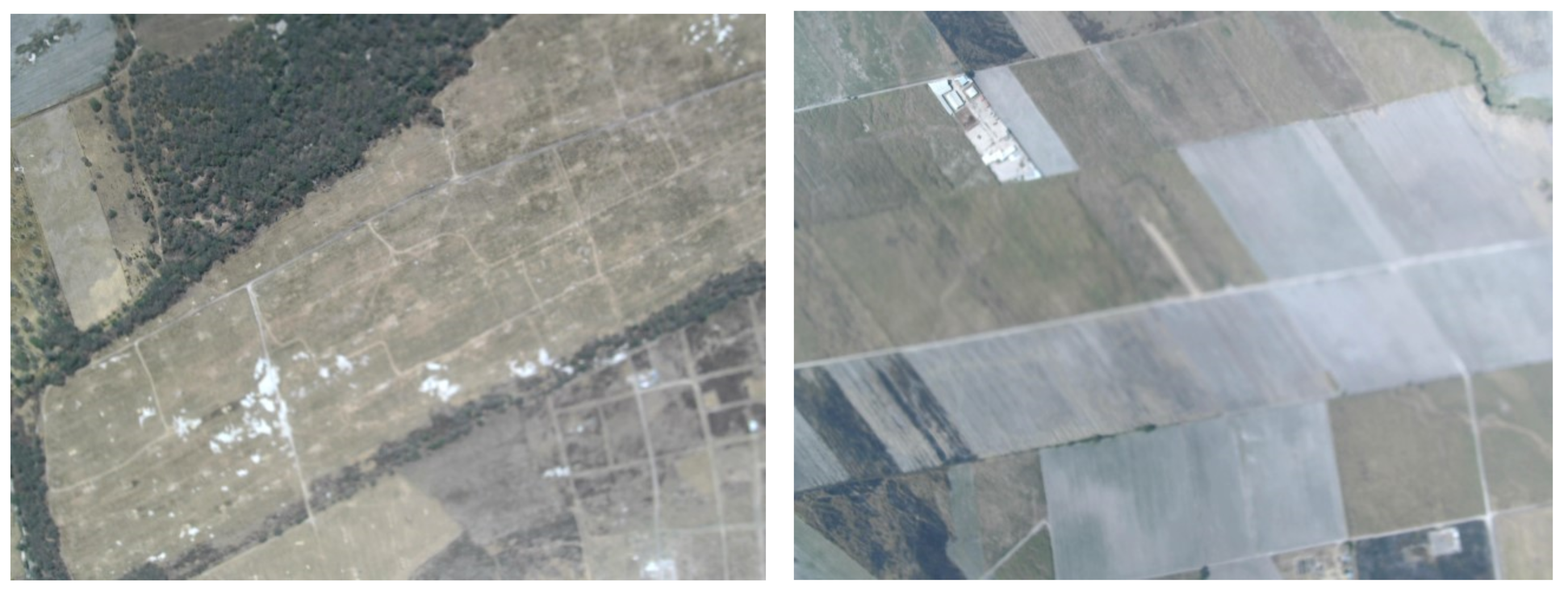
Figure 3.
Flowchart of the algorithm. Two consecutive images are taken, and the displacement between centroids of the keypoints in pixel units corresponding to the good matches is calculated. This displacement is converted to meters and added to the previous coordinate (in UTM). Finally, the result is transformed into latitude/longitude coordinates, and the process is repeated with the next image.
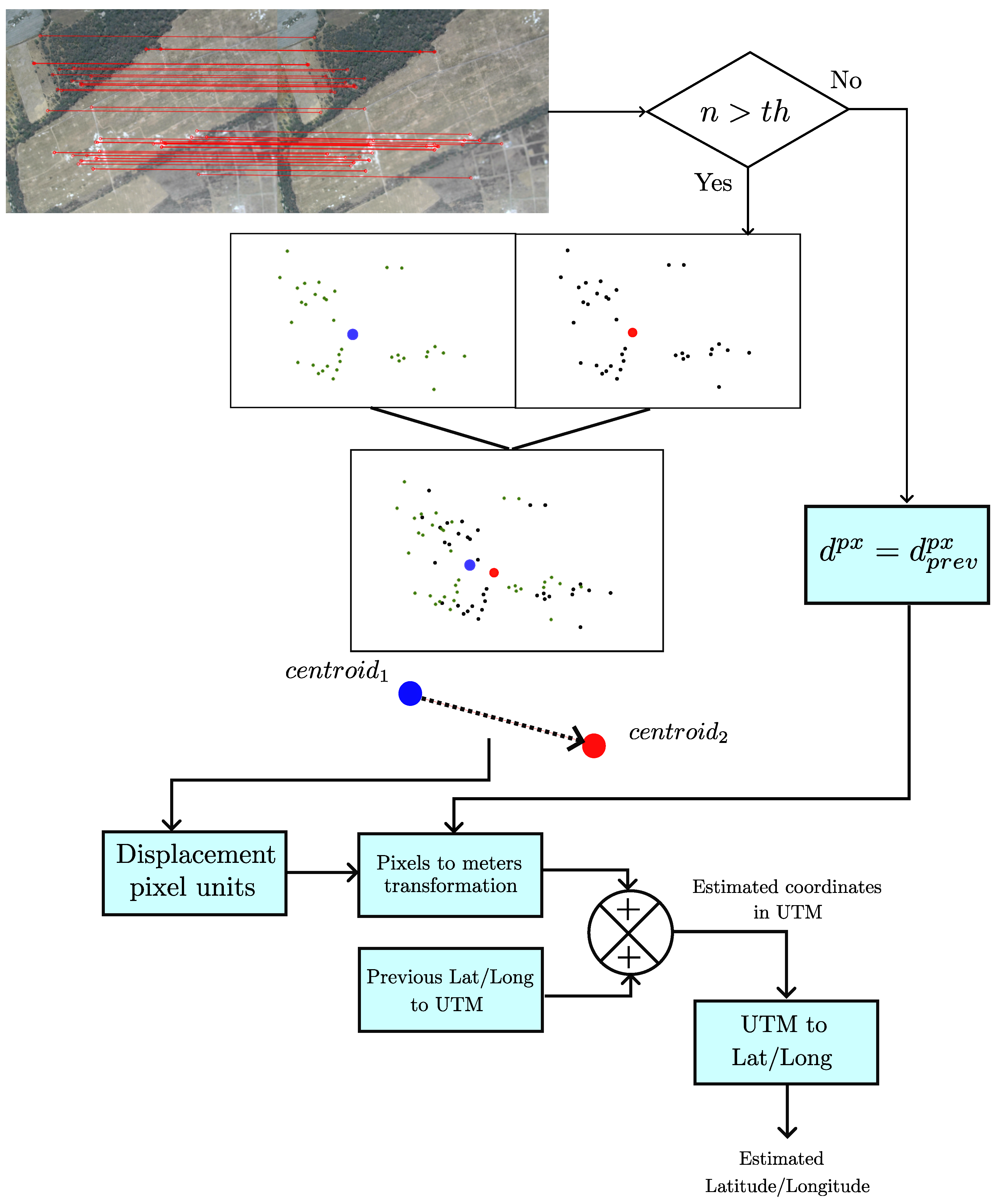
Figure 4.
Matches between consecutive images. The Figure shows the Best 200 matches.
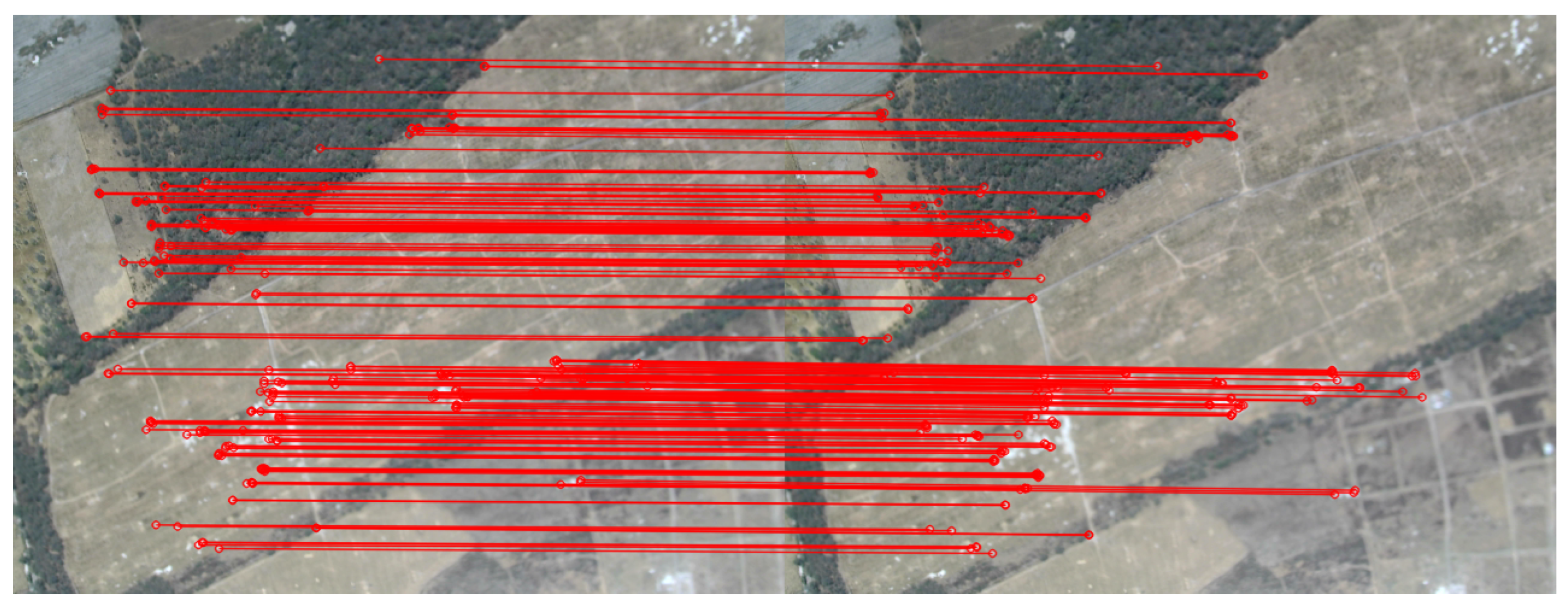
Figure 5.
Matches between consecutive images. The Figure shows matches with
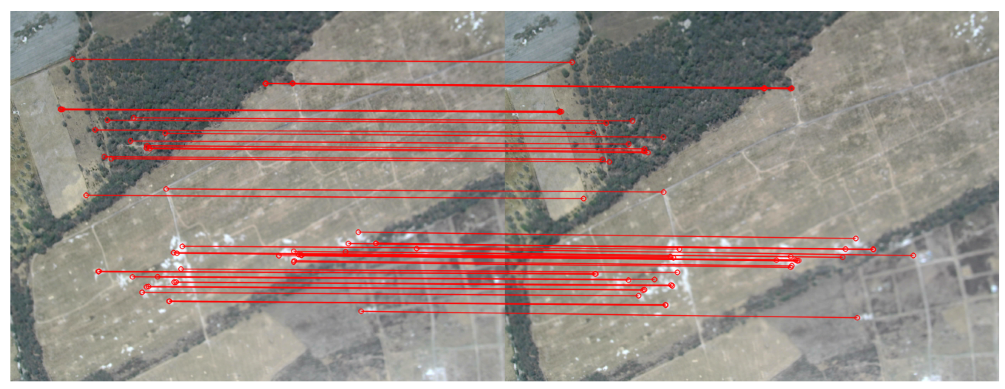
Figure 6.
Elevation map used for these experiments
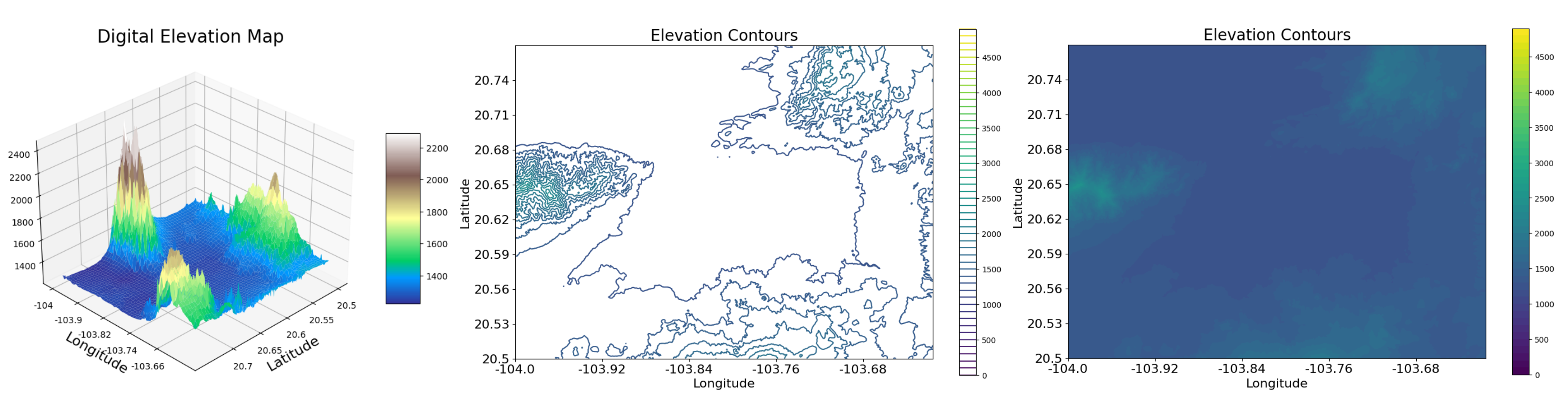
Figure 7.
UTM coordinates system [28].
Figure 7.
UTM coordinates system [28].
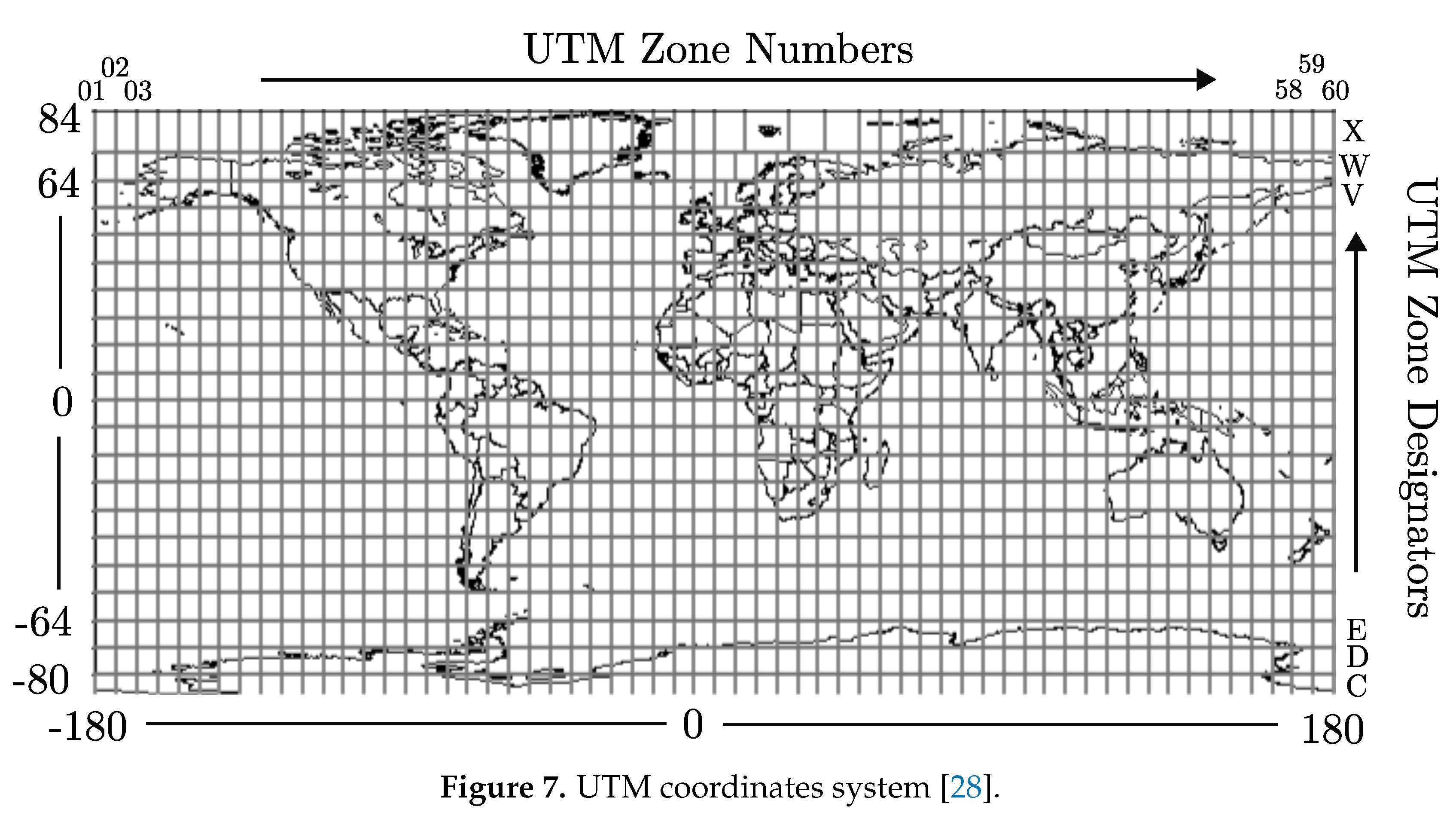
Figure 8.
Output with , ,
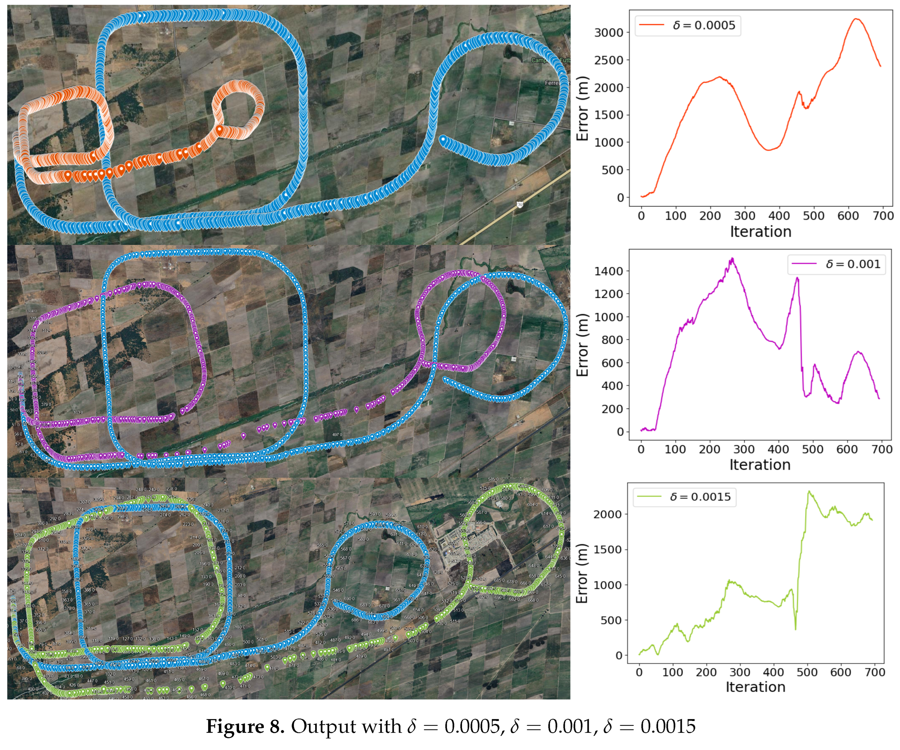
Figure 9.
Pre-processing flowchart. This process ensure to keep the best key-points to compare the real time application.
Figure 9.
Pre-processing flowchart. This process ensure to keep the best key-points to compare the real time application.
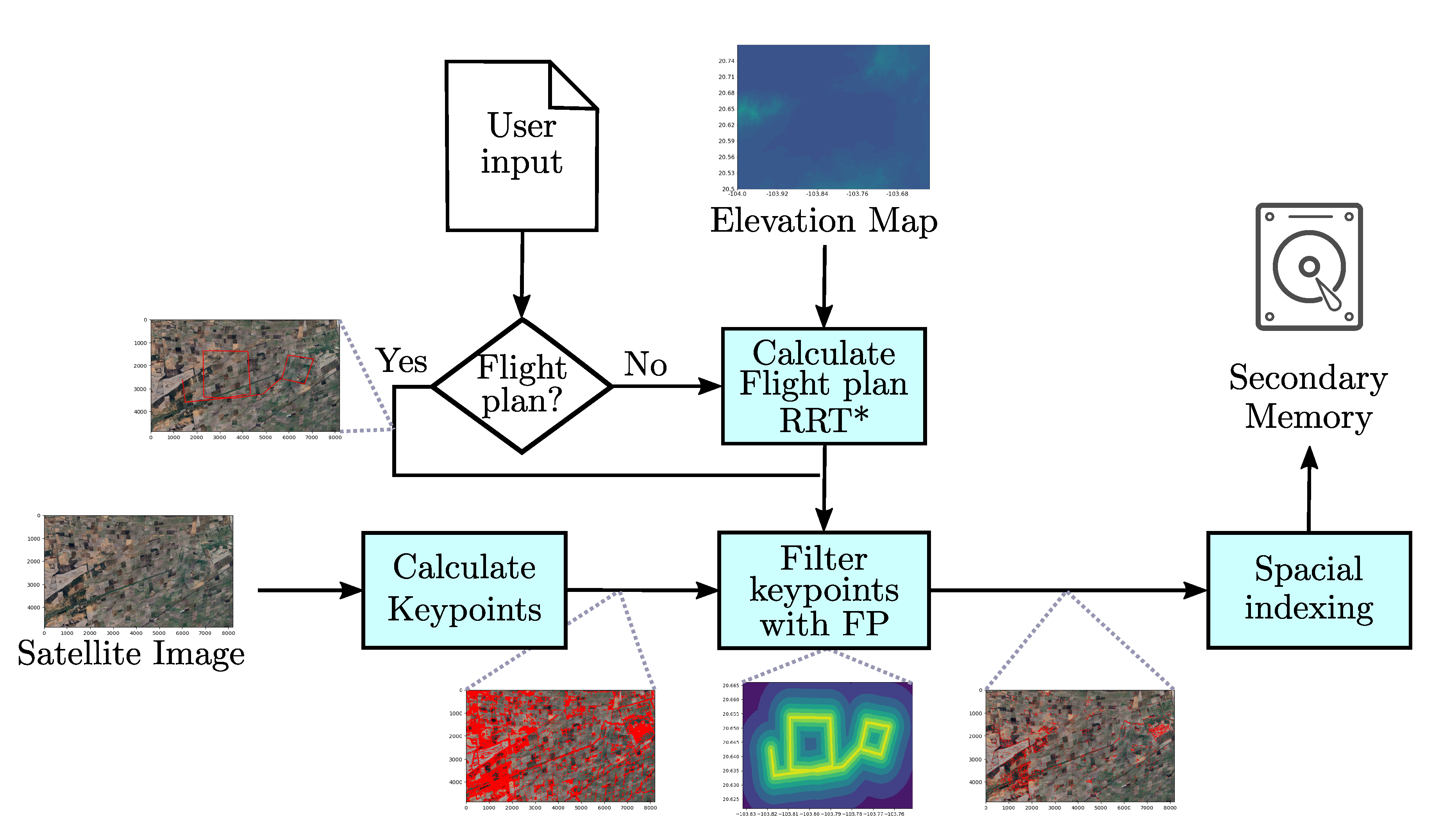
Figure 10.
First example (2D) of RRT* path planning over a section of Hidalgo State in Mexico, we shown the explored paths.
Figure 10.
First example (2D) of RRT* path planning over a section of Hidalgo State in Mexico, we shown the explored paths.
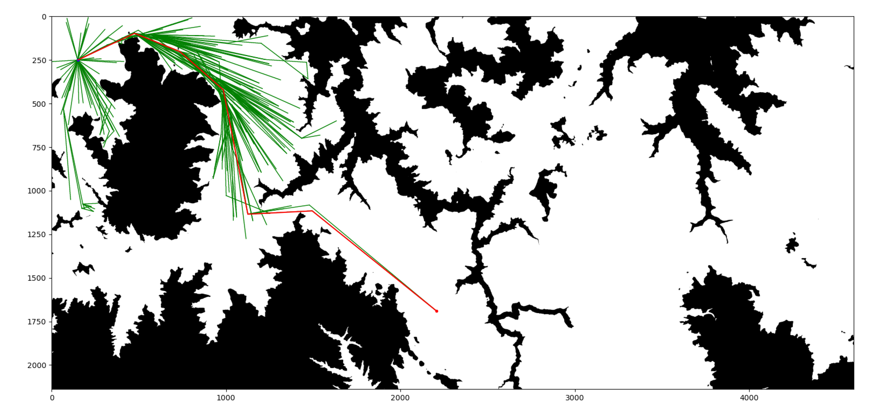
Figure 11.
Second example (3D) of RRT* path planning over a section of Hidalgo State in Mexico, we show the final path.
Figure 11.
Second example (3D) of RRT* path planning over a section of Hidalgo State in Mexico, we show the final path.
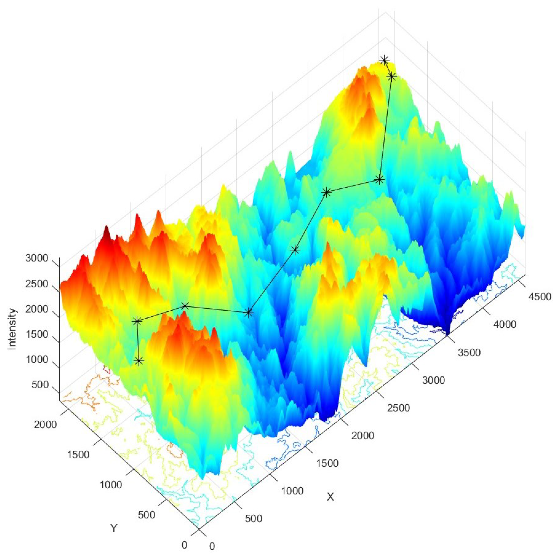
Figure 12.
Key-points of the satellite image
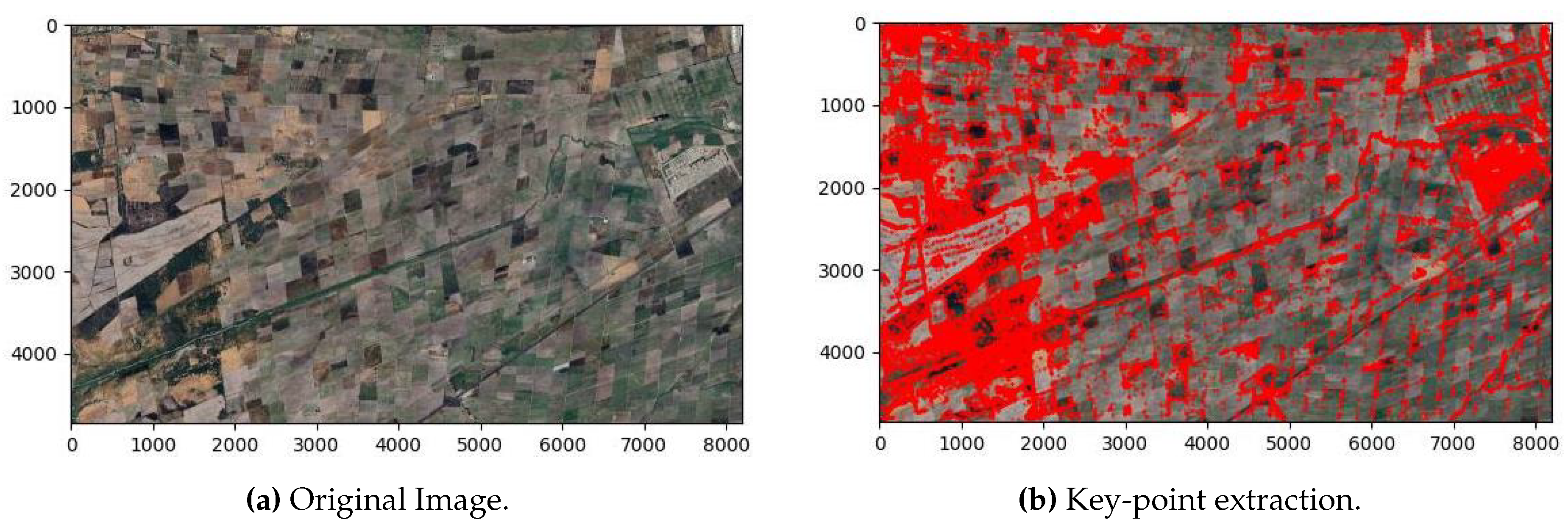
Figure 13.
Key-points of the satellite image
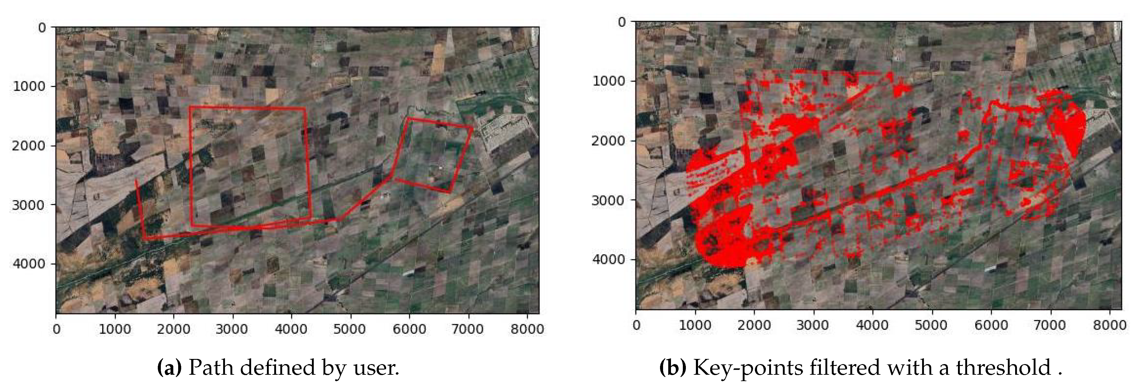
Figure 14.
Distance histogram and its fitted exponential decay probability distribution
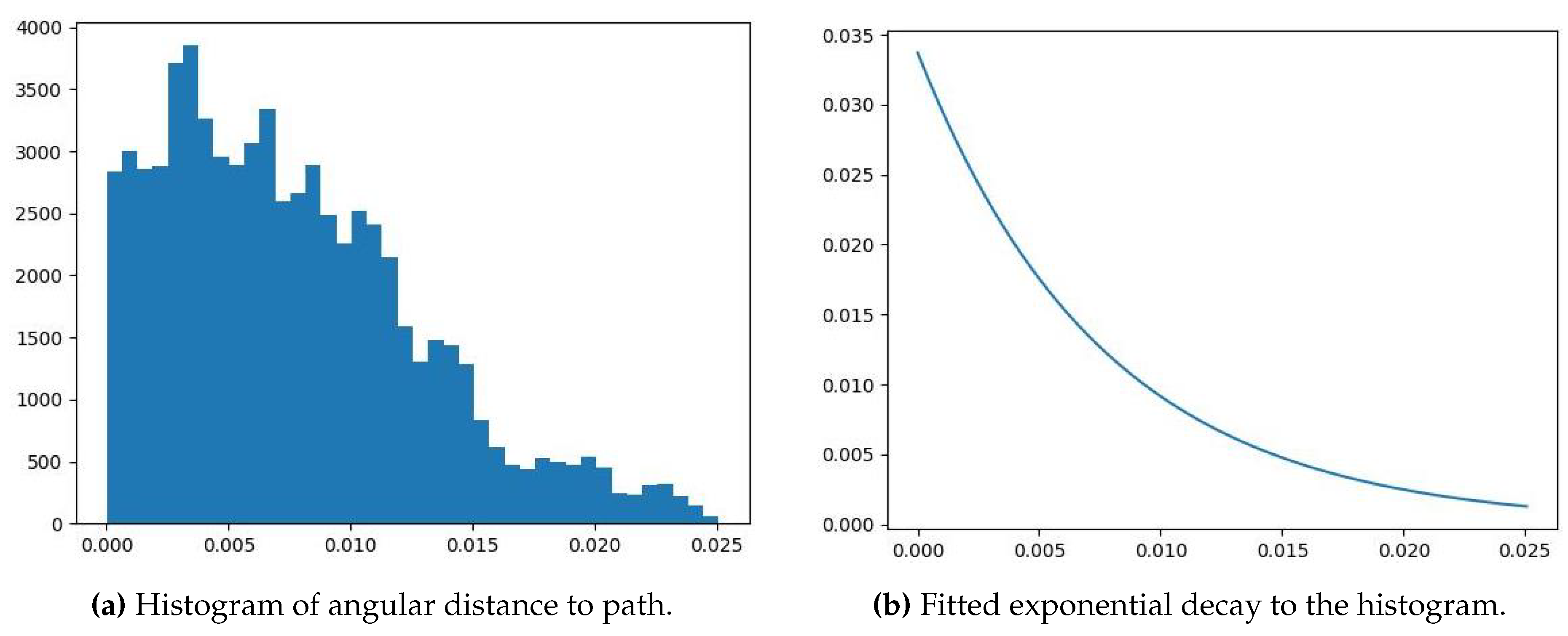
Figure 15.
Map of filtered key-points based on the flight plan
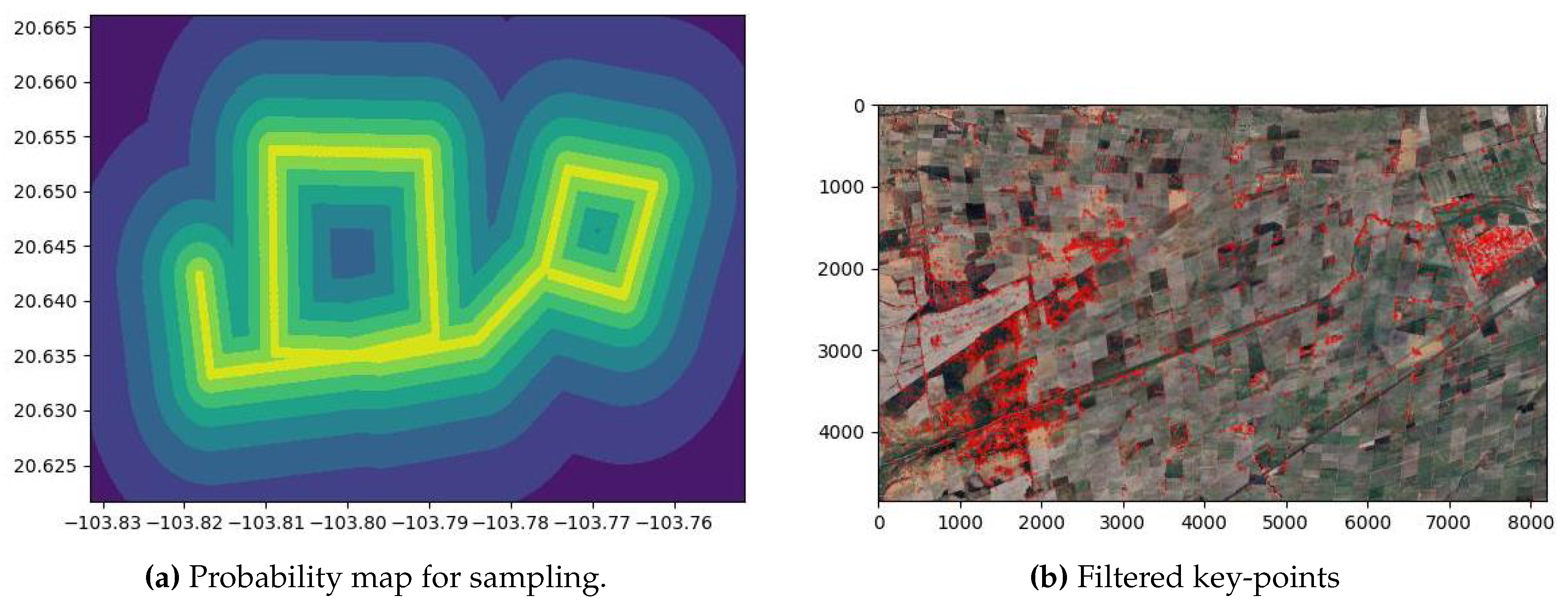
Figure 16.
Quad-tree scheme.
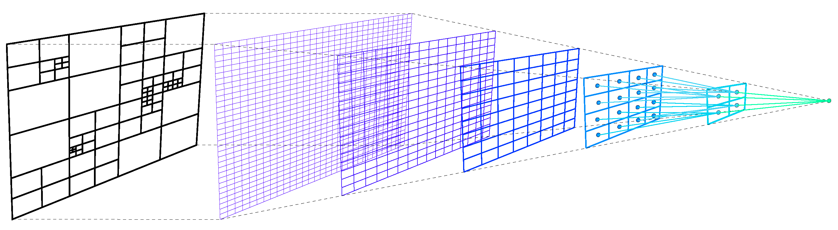
Figure 17.
Offset from the keypoint to the image center.
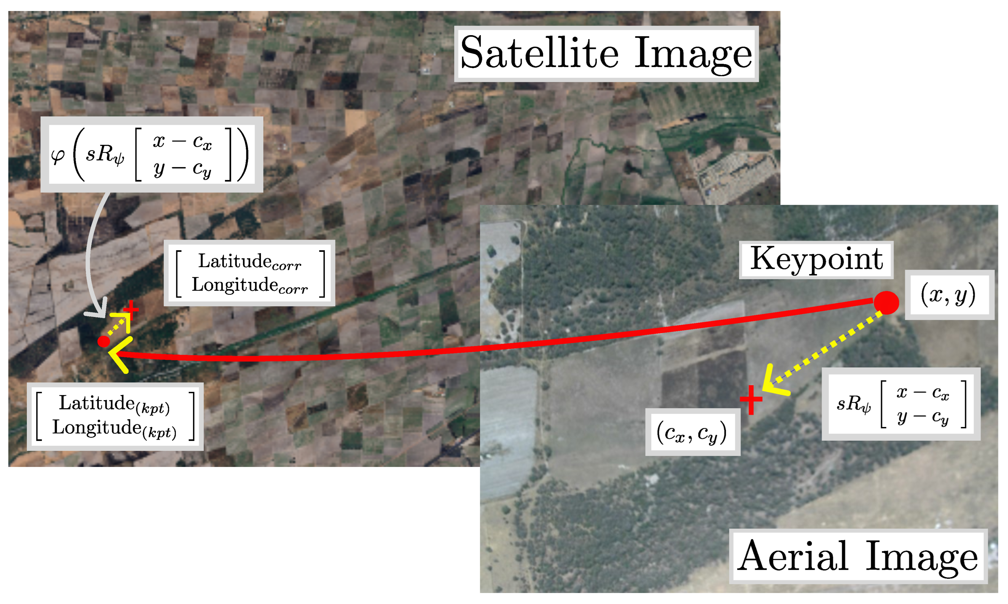
Figure 18.
Our scheme.
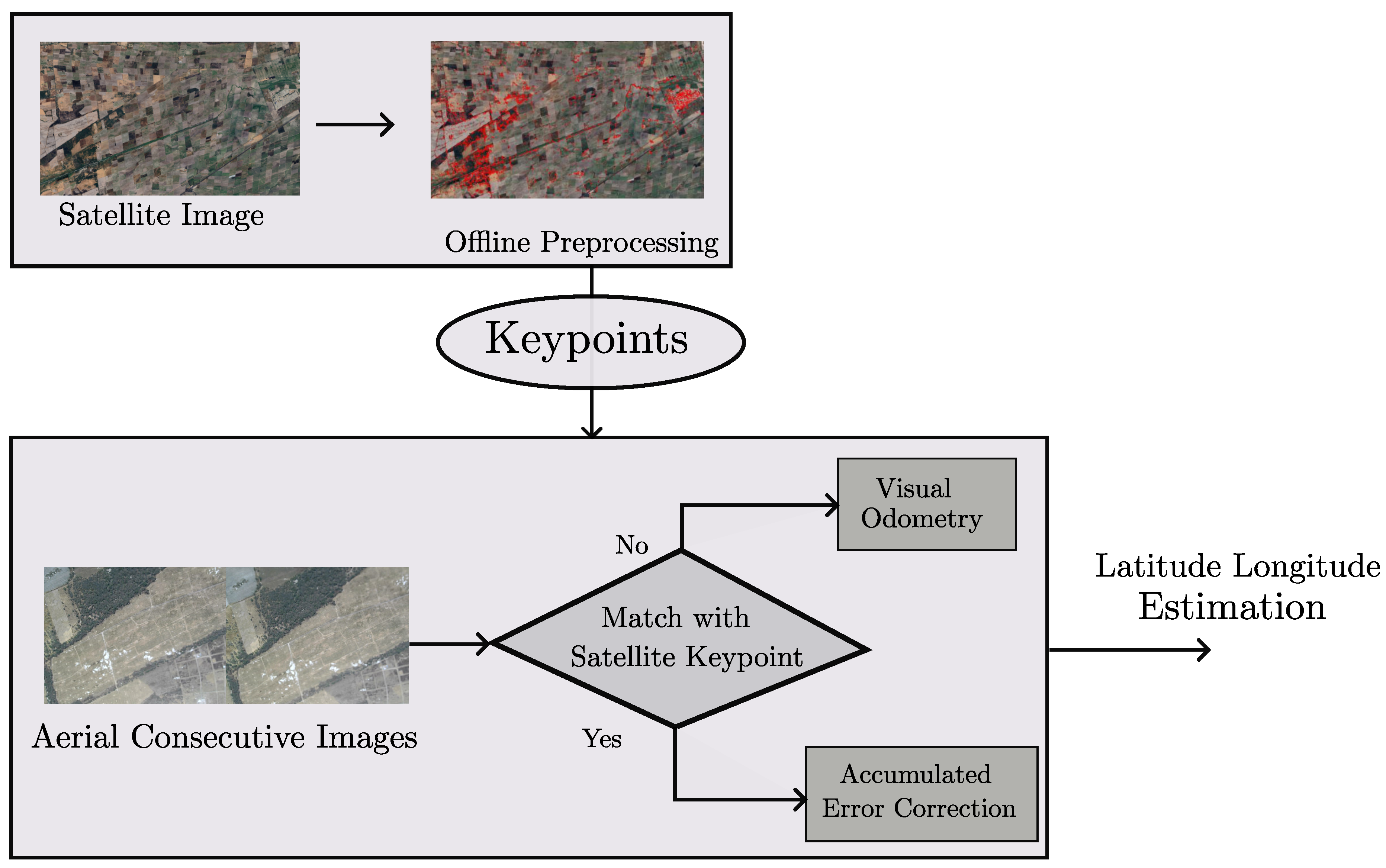
Figure 19.
Output of the correction algorithm.
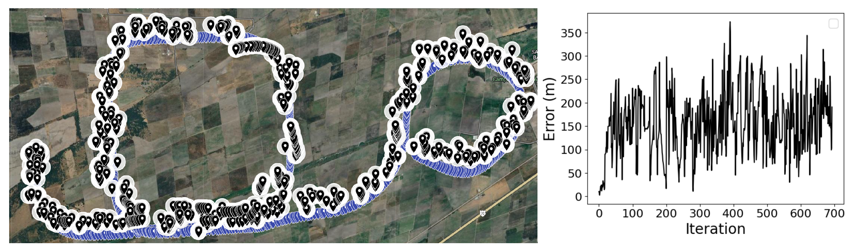
Figure 20.
Filtered output of the correction algorithm.
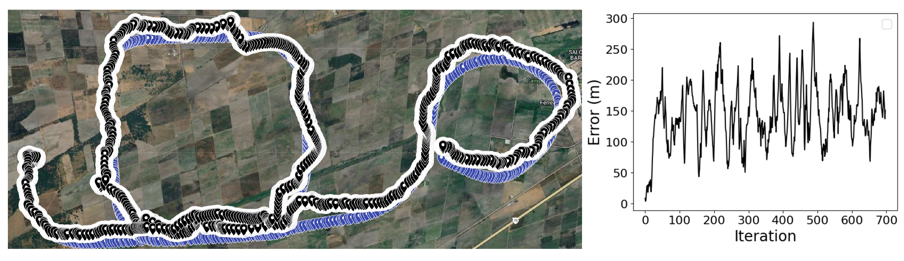
Figure 21.
Filtered output of the correction algorithm.
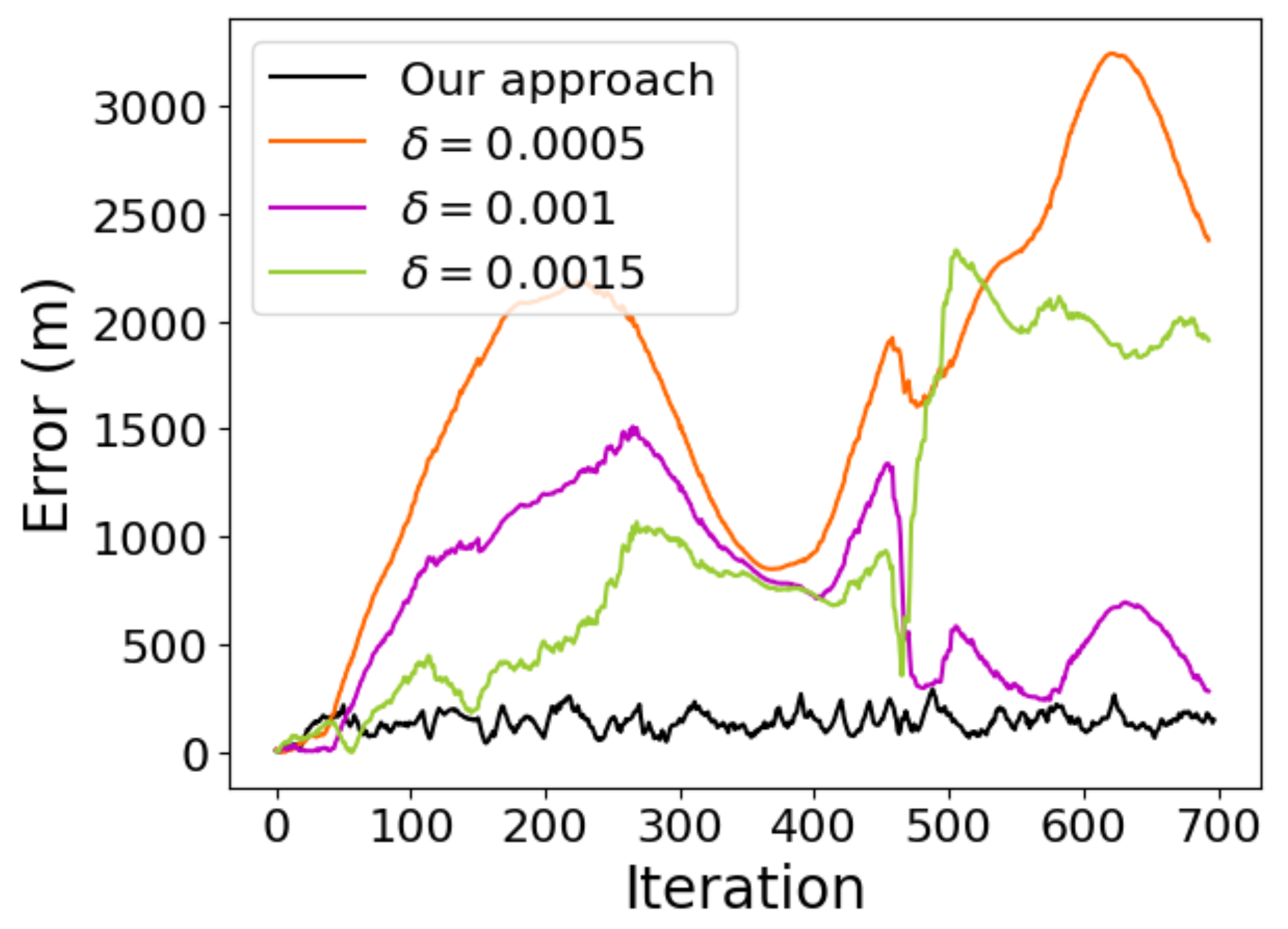

Table 1.
UAV Classification [2].
Table 1.
UAV Classification [2].
| Class | Category | Operating altitude (ft) |
Range (km) |
Payload (kg) |
|---|---|---|---|---|
| I | Micro (<2 kg) | <3000 | 5 | 0.2-0.5 |
| I | Mini (2-20 kg) | <3000 | 25 | 0.5-10 |
| II | Small (<150 kg) | <5000 | 50-150 | 5-50 |
| III | Tactical | <10000 | <200 | 25-200 |
| IV | Medium Altitude Long Endurance (MALE) |
<18000 | >1000 | >200 |
| V | High Altitude Long Endurance (HALE) |
>18000 | >1000 | >200 |
Table 2.
Error comparison in meters (m).
| Class | Accumulated Error |
Root Mean Square Error (RMSE) |
Mean | Std |
|---|---|---|---|---|
| 0.0005 | 1184118.53 | 1893.99 | 1706.22 | 822.20 |
| 0.001 | 516631.52 | 845.68 | 744.42 | 401.27 |
| 0.0015 | 696712.03 | 1230.59 | 1003.90 | 711.71 |
| Our Approach | 99732.63 | 150.79 | 142.88 | 48.19 |
Disclaimer/Publisher’s Note: The statements, opinions and data contained in all publications are solely those of the individual author(s) and contributor(s) and not of MDPI and/or the editor(s). MDPI and/or the editor(s) disclaim responsibility for any injury to people or property resulting from any ideas, methods, instructions or products referred to in the content. |
© 2024 by the authors. Licensee MDPI, Basel, Switzerland. This article is an open access article distributed under the terms and conditions of the Creative Commons Attribution (CC BY) license (http://creativecommons.org/licenses/by/4.0/).
Copyright: This open access article is published under a Creative Commons CC BY 4.0 license, which permit the free download, distribution, and reuse, provided that the author and preprint are cited in any reuse.


