Submitted:
26 April 2024
Posted:
26 April 2024
You are already at the latest version
Abstract
When separation to the parameters of interest appears below resolution limit of the estimator, the ambiguity arises whether two parameter estimates relate to one source emitted twice or two close sources emitted once. In the paper, novel Bayes technique aimed to identify one/two sources below resolution limit by the pair of Gaussian estimates of a source(s) planar location as parameter is developed. Prior probabilities of the hypotheses on one/two sources are available from the analysis of physical characteristics of the emissions, assuming that they can be equally probable. The identifier recalculates a posteriori these probabilities subject to a distance between sources. It is applied to distinguish two location estimates obtained in the planar time difference of arrival mobile communication network. The work of the identifier is studied in the domain of closely spaced network users where covariance matrices of estimates are sufficiently approximated by the constant. The application gives an example of how the identifier revises the prior probabilities and can change thereby the initial preference of a hypothesis with a distance between users in some cases.
Keywords:
separation to the sources location
; probability of estimates resolving
; Statistical Resolution Limit
; Bayesian inference
; identification probability of one/two sources
1. Introduction
Having two parameter estimates the problem to identify whether single source emits twice or two sources at some distance between parameters below resolution limit emit once takes place in application of the resolution methods. The resolution limit of the estimator is described by the Statistical Resolution Limit () defined as the minimal separation at which estimates are resolved correctly [1]. If the separation is less than , then there will exist ambiguity about one or two sources. The concepts of are primarily formulated in the detection theory [2,3,4,5] and the estimation accuracy approach [1], [6,7,8]. Herein, we rely on the estimation accuracy utilizing the Cramer-Rao Bound () matrix-function of parameter, which under mild conditions represents a narrow lower bound on covariance matrix of any unbiased estimator [9]. The equality to is achieved in the class of asymptotically efficient estimators to which we will address in the paper. While true parameter(s) is unknown, can be well approximated by the same matrix-function but taken at parameter estimate to gain its covariance matrix and thereby sufficient approximation of the in the domain of small estimation errors.
We propose novel Byes formalism which can identify one or two sources below by two planar location estimates and their covariance matrices. A handling with positional estimates on the plane is relevant in mobile communication, astrometry, microscopy and many other fields.
The sources have different spectrum, power, others features of the signal but they may be identical. The existing approaches in identifying closely spaced sources typically invoke the probability of number of sources – either from subjective expert experience or as posterior one obtained from Bayes inference, which operates with physical characteristics of the emissions. We come across the closest example of Bayes signal classification in radar [10], seismology [11] and so on, where, having the probabilities of each class for each emission, it is not difficult to deduce probabilities of all possible number of sources for a given number of emissions using probability theorems. In infrared optics, Bayesian calculation is applied to obtain probability of number of neighboring screen images to overcome the smearing effect [12]. A similar problem arises in localization of blinking objects in microscopy where Bayesian Information Criteria are to achieve probability of number of objects for the analysis below the diffraction limit [13]. We will refer to a solution that is able to support the required probabilities of one and two sources as the prior solution (PS). Prior probabilities in the Bayesian formalism will be the ones extracted from PS.
When resolving, the separation to the parameters and is not to be less than some quantitative measure of random distance scattering between their estimates: . For the design of identifier, resolution criteria are reformulated by the means of the notation of the resolving inequality: (RI) in order to catch the probability that distance between parameter estimates is not bigger than . Following this reformulation we propose new concept for planar decoupled estimates when confidence circles of high (near to unity) probability around each of the two parameters are tangent. The concept provides approximately the same probability of the RI () as in scalar resolution criteria in the widest range of covariance matrix spectrum of difference between estimates.
Two mutually exclusive events constitute the Bayesian sample space: confidence circles around each of the sample estimates are either disjoint or intersectional if the distance between estimates is over or below . Bayesian technique recalculates a posteriori given prior probabilities with regard to presumed distance between true locations. Doing that, it can change the probabilistic decision induced by PS. To the best of our knowledge, no solution aimed to discriminate single source emitted twice and two close sources emitted once for a given pair of location estimates, which would be parameterized by the distance between hypothesized sources is mentioned previously.
We illustrate the job of the Bayesian formalism by the example of distinguishing two positional estimates between one and two close each other users, obtained in the basic stations (BSs) network by the means of time difference of arrival (TDOA) technique. The signals are there classified in such a way that probabilities of one and two users can be derived. The solution must answer the following question: does one user emit twice or do two users at varying distance between them, carry out emissions consecutively. The identifier implementation is based on the radius of high confidence circle obtained in the paper for the confidence probability of 0.99. This radius will subsequently be denoted as .
The paper is organized as follows. In Section 2 the resolution criteria are surveyed. The problem is described in Section 3. New concept of is founded in Section 4. Section 5 contains the design of Bayesian identifier. The algorithm for estimation of is presented in Section 6. The application of the identifier in the BSs network is quantitatively studied in Section 7. Section 8 briefly draws the summary of the paper.
2. The Works Related to Resolution Criteria
One of the earliest was Lee resolution criterion [6] for scalar decoupled estimates, in our reformulation , , , , where , are standard deviations of estimates , , which provide the resolving with “high probability” due to big factor : it is evident that the bigger is chosen, the higher the probability is that a separation between estimates is not bigger than (authors referencing to Lee consider ). Delmas and Abeida [7] expressed via standard deviation of the estimates difference: , hence the probability of the inequality is smaller than with Lee, because inequality being satisfied even at . Regarding coupled estimates, Smith [1] offered , , where has been interpreted in [8] as an element of extended matrix by using the change of variable formula. Both and are articulated in standard deviation of a difference between estimates. This fact offers an opportunity to achieve in a scalar case for a known distribution of estimates.
In the work of Korso, Boyer, Renaux and Marcos [8] the general problem for multiple estimates was considered. Therein, , where separation between sets of parameters is the -norm distance (Minkowsky distance). Let us represent two scalar parameters , in a vector form, and denote estimates of vector obtained from the decoupled emissions 1 and 2 as , respectively. Then, the RI is written for coupled estimates in metric of 1-norm () of a difference vector as ,
, where variances and covariance of estimates are defined by the means of underlying functions at true parameters and , which are obtained by applying change of variable formula to the extended measurement model of the estimator. The result distinctively extends scalar on vector case, however , i.e. the probability of , could hardly be determined here in comparison with scalar resolution criteria.
Clark [14], analyzing the resolution of estimator that produces vector decoupled Gaussian estimates, presented the metric of a distance between ellipsoidal confidence regions of probability 0.9 around each of the two parameters. The estimates are resolvable when ellipsoids are disjoint. of the estimator is the metric from which they are tangent.
In the study, we transform Clark’s idea about the ellipsoidal confidence region to develop the concept of based on circular one of high confidence probability which is probabilistically consistent with conventional resolution criteria [1,7]. As with Clark, the estimates will be resolvable when the circles are disjoint, but their tangency will correspond to the equal to the sum of their radii.
3. Statement of the Problem
During the two consecutive time intervals and , , signals from emission I and signals from emission II are received. The th signal depends upon vector parameter , , which gathers physical characteristics of the emissions, and dimensional measurement parameter which is known smooth function of two-dimensional unknown vector of the source location, :
where is a waveform vector-function of time and parameters , ; is unbiased noise with for the all , denotes mathematical expectation operator.
Unbiased estimator establishes the inverse connection between signals (1) and related to emissions I and II measurement vectors and , , :
where and are the measurement errors corresponding to emissions I and II with , i.e. and are decoupled.
Unbiased estimator uses measurements (2) to produce estimates and over emissions I and II: , , , , where and are the corresponding errors, which are also decoupled.
We consider (a) “regular enough” algorithms and such that and are both normally distributed [15]: N(,), N(,) with a given covariance matrix of estimates and an unknown one of estimates . The estimators and are assumed (b) to be efficient, hence is calculated as by use of Fisher Information Matrix : . For Gaussian noise, .
Hypotheses and serve to specify the sources of emissions: hypothesis means that one source at with emits twice, hypothesis – that each of the two sources at and with and emit once. The probabilities and of the hypotheses come from a preceding step of data processing where parameter can be involved.
We define the circles and , denotes Euclidian norm, with radii and where estimates and fall with high probability : for and , for . Due to negligible probability of outliers beyond circles we will treat estimates and so that as if , or , . Assumption (c) on small estimation errors is quantified inside the confidence circles as at and at .
The identification is performed in the area where positions and will be placed at the distance of not more than , where , . We take the assumption (d) that is sufficiently approximated by a constant for the all locations from the annulus . Thus, it is permissible to use in that area sample estimates and of and for the calculation of sample approximations , of unknown true covariance matrix or matrices. As shown in the application, the stronger condition will be there fulfilled in the specific domain of closely spaced sources with a good accuracy.
Our purpose is to find the probabilities of that estimates and refer to one source in position and two sources in positions and for a given separation on conditions (a), (b), (c) and (d).
4. Concept Based on High Confidence Circle
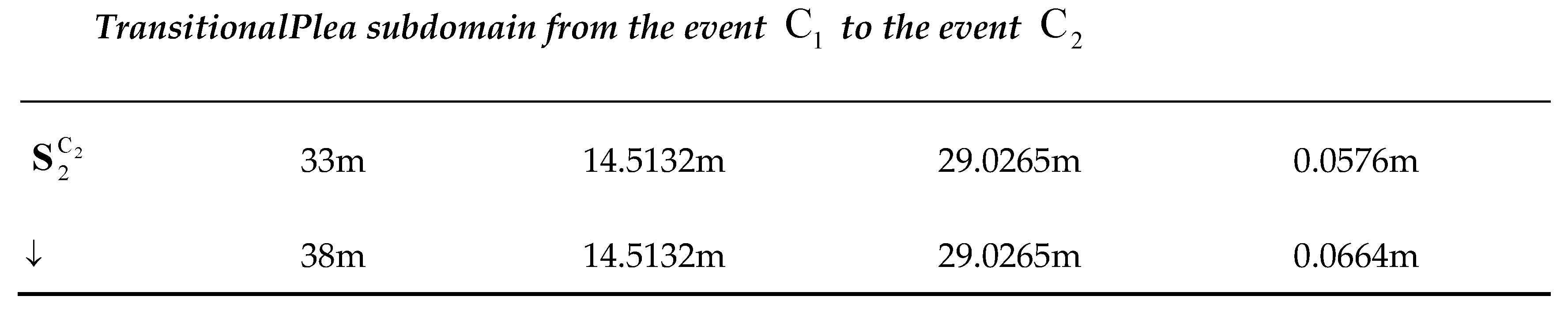
In the frame of this Section, random variables and are considered as just the Gaussian two-dimensional estimates, not necessarily of location coordinate, with and . The difference between estimates , , , is Gaussian with a mean and covariance matrix with eigenvalues . We propose the concept of based on a tangency of two confidence circles and of probability when , which comes from the following Theorem.
Theorem.
Proof of Theorem.
1. The region encompassing where falls with probability in polar coordinates , originated correspondently in and is , , and , . The squared distance from to any point of is maximum of which is achieved at , for and is equal to . Consequently, is a circle centered at with radius and bounded by the circumference including origin of coordinates.
2. The region where variable falls with desired probability is formed by the intersection of the circles and , so long as , see Figure 1a. Straight line connecting the intersection points of corresponding circumferences and is collinear in virtue of symmetry to the tangent to at the point . It divides the line from origin to on two identical segments, hence the angle is equal to , see Figure 1a again. We successively translate in origin and rotate coordinates to obtain probability integral for in terms of spectrum of . Changing to polar coordinates (,) we get
where . The ordinate divides on two semicircles and , but two identical regions and associated with complement to semicircle , Figure 1b. From the symmetry of probability density in integral (3) with respect to angle one has and .
3. We represent probability (3) as
where , see Figure 1b again.
Performing the integral in (4) over variable leads to
We maximize it over to evaluate from below:
It can be easily verified that the derivative of the exponential function from (5) is non-positive, thus required maximum is achieved at and is equal to . We substitute with in exponent and perform integration in (5) [16] to achieve the inequality
where . The expression in parentheses with exponent is the probability that realizations of will be in the concentration ellipsoid centered at origin with principal semi-minor axis and semi-major axis . Region which contains with probability is the circle inscribed in the ellipsoid, so its confidence probability will be closer to unity than . And if so, we substitute it with unity and end the Proof □.
Proceeding from the Theorem, we establish in RI ensuring , low bound of which depends on spectral characteristic . Function is monotone decreasing by : it approaches at , hence when . In other hand, it approaches zero at , hence . Since, say we get and can declare that occurs here in a proximity of . When concentration ellipsoid is degenerating into the circle with radius yet therefore the contribution of in probability is in fact . On the contrary, at it elongates along the semi-axis , , and hereby approaches zero.
5. Bayesian Identification Formalism
Sample analogues and of one or two true covariance matrices are employed to achieve the approximation of as where estimates , approximate twice or , once. Bayes sample space is defined to consist of two events, when the confidence circles encompassing sample estimates and intersect: at or do not intersect: at . Probabilities of the events and are: and , and . Probability is very near to unity thus is very near to zero. Probability decreases asymptotically with the rise of while asymptotically increases. We define all possible on the circumference in order to pass from unknown to its minimum and maximum on . To develop Bayesian scheme we need the following Lemma.
Lemma. , at , and , at .
Proof of Lemma. For the pair of some vectors and , where , one has and , and , . Variances of and are increased by factor and correspondently as compared to the variance of , hence due to the properties of Gaussian distribution and . Thus, and that completes the Proof □.
As comes from Lemma, is smaller than and approaches it from below at ; both and decrease monotonically with the rise of while and monotonically increase.
We apply binary Bayesian theorem to construct maximum and minimum of the posterior probability of two sources,
and minimum and maximum of the posterior probability of one source,
The preference of a hypothesis at small depends on which probability, or is bigger: if a) then , otherwise b) . Both (6) and (7) decrease as goes up while probabilities (8) and (9) grow. Hence, hypothesis becomes more and more probable with from zero up to , while hypothesis is less and less probable. Starting with a certain , we get for the case a) that but still , at which preference is ambiguous, however with a further increase in hypothesis begins to prevail, . For the case b) hypothesis prevails at all . As , probability is much bigger than even though for sensible prior probabilities.
We define for identification probabilities (IPs) of one and of two sources if , and , if . IPs are not defined if when a hypothesis could not be preferred. As for , and . To achieve preference the function of relative difference between IPs is compiled:
which is compared with a threshold . At preference is ambiguous. If or then hypotheses or respectively prevail. When we select .
Probability distribution of squared distance between two Gaussian vectors (in our case it will be ) is referred to the distribution of a quadratic form , where is non-central Gaussian vector with a mean and covariance matrix (for us ), is symmetric and nonnegative definite matrix. We obtain the desired distribution by equating to the identity matrix. Although its mathematical structure is complicated, modern computer resources allow implement supporting functions precisely [17].
The separation is to be chosen everywhere in the range of for the event or of for the event in the use of identifier (10). Nevertheless, when it approaches probability of both events may grow nearer to , where they tend to be equally probable. To improve identification reliability we invent the probability threshold if necessary for determining such distances or that would afford a more valid event: for or for . Beginning from we decrease the distance up to or increase it up to . Probability is assigned to be the probabilistic measure of event validity, which prescribes that events at or at , are both valid with probability no smaller than . The region of is defined to be of invalid event.
To summarize the results of Section 5 we present the core pseudo-code of the identification procedure:
if then
Step 1. Identify one/two sources at
if
then No preference of a hypothesis else
if thenPrefer
else ifthenPrefer
else No preference of a hypothesis
end if end if end if
else //
Step 2. Identify one/two sources at
if thenNo preference of a hypothesis
else Prefer
end if end if
6. Estimation of
The topic of a confidence circle has been addressed in a number of publications regarding circular error probability () integral [18,19,20,21,22], occurring in navigation and surveillance systems. is the radius of a confidence circle which contains a random variable with probability .
The probability density for zero mean bivariate Gaussian variable with covariance matrix is defined as
where , and are standard deviations and covariance of and . Hence, function (11) is
where is a correlation coefficient.
Among others, Krempasky estimator [22] is the most attractive both owing to its numerical simplicity (it is closed-form) and high accuracy (the deviation of estimate from the exact value is less than 2 percent). Krempasky first rotates the and coordinates by the angle : such that in transformed coordinates and . Correlation coefficient is in the new coordinates. With polar coordinates the originating in (12) integral for , expressed through variables and , is written with angular coordinate after the integral over radial coordinate is performed:
The integral (13) is then expanded to the fourth order in the correlation coefficient , and after much manipulation the final estimate is found to be
We substitute with in (13) to rework Krempasky estimator to estimate . Repeating the same manipulation as in [22], one can make sure that estimate is deduced from (14) by substitution with . Finally, the expression for is derived:
To assess the performance of we propose the alternate estimate based on the two specific behaviors of the integrand (11) in Gaussian probability integral in the vicinity of zero and beyond. Initially, it is reformulated as an integral along one variable [23]:
where are eigenvalues of , ; is a modified Bessel function of the first kind and zero order. It is approximated with the use of the asymptotic expansions [24]:
Equation (15) is now rewritten as , at (i) or as , , at (ii). The integral for the case (i) is the probability which is bigger than or equal to , hence , otherwise for the case (ii) – . We use representation from (16) at instead of in integral to get its approximation and afterwards. If then case (i) is recognized, or otherwise – case (ii) for which representation from (16) at is used instead of in integral to achieve approximation . By doing so, we come to the approximation of the right part of (15) and obtain:
where is the same approximation as with instead of . The integration techniques detailed in Appendixes lead to the following analytical expressions:
see Appendix A, and
see Appendix B, where ; and are the orders of approximation. As the member in is small as compared to and further ignored.
We assign in after that case (i) is reduced to the following equation for :
As it is observable, the derivative along of the function from the left side of this equation is negative, supplying the solution uniqueness.
For the case (ii) we set in and obtain the closed-form solution:
The performance of estimate versus is studied by simulation in the full range of from -0.0098 to 0.9888, which correspond to varying of the correlation coefficient and sigma ratio (ratio of smaller to larger standard deviation) in the intervals (-1,1) and (0,1) respectively. The performance index for comparison is the probability integral (15) performed numerically with estimates and . Table 1 contains the extraction from the simulation results.
As we can see from the Table 1, at radii and are both of excellent accuracy and close to each other. As approaches zero from below, estimate keeps excellent accuracy while estimate degrades. The bigger after zero is, the better becomes, while degrades gradually. It is safe to conclude, that estimate begins to outperform visibly from the onwards. As a result, radius is estimated as follows:
7. Distinguishing Two Estimates between One or Two close users in the TDOA BSs Network
Bayesian formalism is applied to distinguish two positional estimates of the user(s) which are obtained in the TDOA planar positioning network. The received signals are classified by parameter with the probabilities and over emissions I and II, where is the number of different users. Proceeding from these probabilities, one can easily get and .
In TDOA technique, output signal at -th BS is with parameter () of time difference of emission arrival on that BS and reference one, placed in (0, 0), from a user located at : , , , where is the speed of light. The model (1) is here reduced to the following one:
with scalar signals, waveforms and noises instead of vector ones as in (1) at . Scalar processes , and function with are given at reference BS.
If signal at each of BSs is uncorrelated with the signal at reference BS: , as maximum likelihood estimator is efficient asymptotically [25]. As far as is concerned, the constrained weighted least square estimator [26], which combine core pillars of the quadratic and linear correction techniques [27,28], is to be efficient for uncorrelated measurement errors of parameters , . Despite the fact that they nevertheless correlate through signal at reference BS, it is presumed that matrix is to be near to a diagonal one. Reasoning from the aforementioned, the covariance matrix in TDOA BSs network is calculated as
There are five BSs, including the reference BS. Four BSs in conjunction with the reference one, produce the range differences of arrival , corrupted by the noise with standard deviations ====0.04m (m hereinafter refers to meters). They are situated at (1000, -700)m, (-1000, 2000)m, (4000, 3000)m and (-4000, 1000)m. The identifier is investigated in the close users domain (CUD) to be associated with the position at (14000, 12600)m.
Since the exact solution for the distribution of [17] is very expansive, the simpler closed-form Lui-Tang-Zhang approximation [29] is utilized in the study.
7.1. Characterization of the CUD
We intend to construct the CUD around in such a manner to characterize it by the constant characteristics and which would be sufficient approximations of , where and are the radii of the confidence circles and centered at and in charge of probability 0.99, and for the all from CUD. The estimates cover subdomain when locations fill . Event would predictably be observed in . To get event we have to withdraw from the subdomain into the subdomain where is bigger than .
In the simulation, is computed at points evenly spaced along circumference of radius centered at : , . Thereafter, mean values , and the square root from the mean of squared deviations of from , are determined.
We start with , as a result of which , are obtained. The next distance is to find with and compare it to : if is nearly identical to then the circumference of radius will be the boundary of subdomain characterized by the with the accuracy . With regard to the subdomain , , are computed at some and at . If and are nearly equal to , then we acquire at the subdomain and at entire CUD characterized by the , wherein is the worst approximation accuracy of in CUD by the constant.
The simulation results for =1000 with equal to 14.5133m are given in the Table 2.

Table 2.
CUD characterization on.
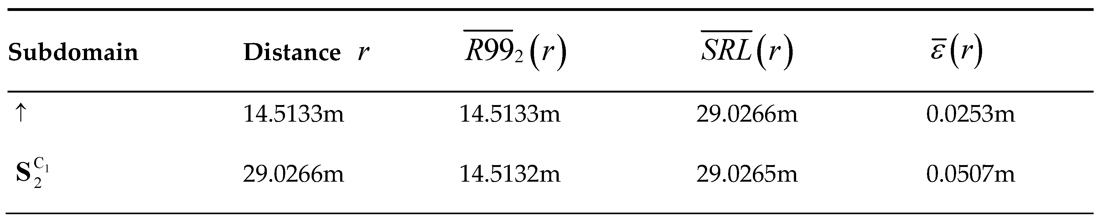
Taking into consideration the column from the Table 2, we can infer that [28.9601, 29.0929]m. Having interval centered at where true is varied, we accept it to be constant, namely 29.02m with the accuracy 0.07m. Thus, is approximated in CUD by the constant with a good accuracy. Therefore, we have reason to approximate the true covariance matrices by the constant everywhere in CUD as well. To this end, the mean of over 1000 points evenly spaced along the circumference of radius , , and the mean are computed. To reveal the scattering of towards in CUD we additionally determine the matrices , , where , correspond to the minimum and maximum of on the same circumference: , . Simulation data in square meters are: , , hence ; and . Following the same logic as in characterization on , we approximate in CUD by the with the accuracy . Spectral characteristic of the is equal to 29.3636, hence .
7.2. Identification in CUD: Simulation and Discussion of Results
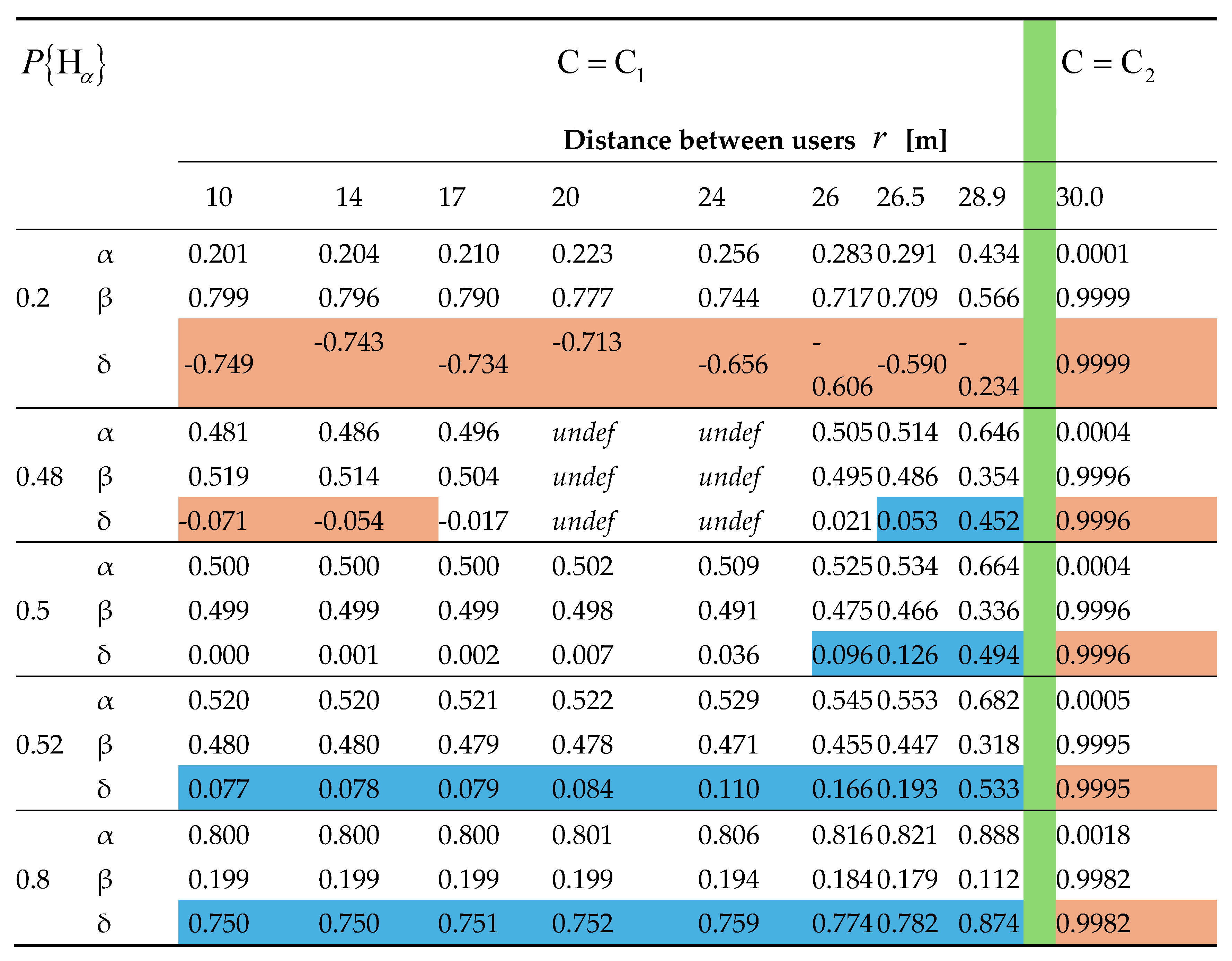
There is no need to employ the estimator [26] in the simulation because the CUD is already structured into the subdomains and where all the estimates fall. We use and established previously in Subsection 7.1 of this Section to find IPs and build the identifier function under prior probabilities =0.2, 0.48, 0.5, 0.52, 0.8 related to the probabilities =0.8, 0.52, 0.5, 0.48, 0.2 and compare it with the threshold =0.05. The threshold for valid events is =0.55 under which region of invalid event (28.90, 29.76)m is determined. The results of simulation are shown in Table 3, where α, β and δ denote the rows for IPs , and identifier function respectively; abbreviation “undef” denotes undefined IPs and .
In the Table above the fragments of rows δ that are colored blue conform to the one user identification, those colored brown conform to the two users identification, and the uncolored ones do not conform to any identification. Green column is to highlight the region of invalid event. Figure 2 visualizes identification probability from Table 3.
To facilitate the analysis of the simulation results from Table 3 we consider two different users, = 2.
When =0.2 one has high probability =0.8 that two users emit due to high probabilities and , as in the example =0.125, =0.875, =0.9, =0.1. Although decreases with separation from 0.8 to 0.566, it still remains big enough in the subdomain till 28.9m to identify two users. On the contrary, for the probabilities =0.875, =0.125, =0.9 and =0.1 one user emits twice with probability =0.8, most probable user 1 ( = 0.775). rises with separation of two hypothesized users in from 0.8 to 0.888. Probability = 0.48, which may be provided by the collection =0.4, =0.6, =0.6 and =0.4, is slightly less than probability 0.52. However,
decreases with separation from 0.52 to 0.514 at 14m where two users are identified. As , the preference at 17m becomes ambiguous. grows up to 0.505 at 26m, but as and in the region of [20, 24]m IPs are undefined, the identifier is not there able to select a hypothesis. Since 26.5m up to the 28.9m one user 1 or user 2 (=0) is identified with probability from 0.514 to 0.646. The identifier changes here the prior preference on two users in favor of one user with growth of separation. Probability =0.52, say for =0.6, =0.4, =0.6, =0.4, is slightly bigger than =0.48 but grows with providing the identification of one user everywhere in with probability from 0.52 to 0.682, little bit more probable of user 1 (=0.2). The case of equally probable hypotheses, =0.5 at =0.5, takes place rather when it is hard to classify the emissions. For the separation up to 24m the growth of is negligible. However, for bigger separation from 26m up to the bound of one user is identified with probability from 0.525 to 0.664, user 1 or user 2 (=0). Even though prior preference is uncertain, the identifier comes to hypothesis with the rise of .
In the subdomain
where the separation is not less than 29.76m, two users are identified with near to unity probability regardless of the prior probabilities. We could interpret this as follows: at =0.8, 0.52 – two different users, at =0.52, 0.8 – user 1, at =0.5 – one and the same or different users for our examples of the classification probabilities. Transitional subdomain between Bayes events is the one of the invalid event where the identifier is incapable to work.
8. Concluding Remarks
Novel Bayesian formalism aimed to identify under double emission one or two closely spaced sources parameterized by their separation, through the use the two location estimates and their covariance matrices, is designed. Prior probabilities of the hypotheses on one and two sources are extracted from the prior solution (abbreviated as PS in the paper), assuming that they can be equally probable. The job of the formalism below and over resolution limit of the estimator is supported by the new resolution criterion emphasizing the probability of the resolving of planar parameter decoupled estimates.
As illustrated in the application, identification technique revises the probabilities induced by PS in dependence upon the distance between sources: if prior probability of a hypothesis is large enough, the identifier only recalculates the initial probability below resolution limit leaving PS-decision unchanged; if prior probability of one source is equal to or slightly less than one of two sources the identifier can change with distance the PS-decision in favor of one source; two sources are identified over resolution limit irrespective of PS-decision with near to unity probability where the identifier works as a routine resolver.
In the future we plan to extend proposed technique on a more general problem of identifying the number of sources, each of which can emit one or several times by a given set of location estimates.
Funding
This research received no external funding.
Institutional Review Board Statement
Not applicable.
Informed Consent Statement
Not applicable.
Data Availability Statement
Not applicable.
Conflicts of Interest
The authors declare no conflict of interest.
Appendix A. On Integration of
Integral is equal to
Applying to integral the rule of by parts integration we conclude that
Appendix B. On Integration of
Change of variable in integral leads to
The integral is performed by parts:
References
- Smith, S.T. Statistical resolution limits and the complexified Cramer-Rao bound. IEEE Trans. Signal Process. 2005, 53, 1597–1609. [Google Scholar] [CrossRef]
- Abramovich, Y.I.; Johnson, B.A.; Spencer, N.K. Statistical nonidentifiability of close emitters: Maximum-likelihood estimation breakdown. In Proceedings of the 17th European Signal Processing Conference, EUSIPCO 2009, Glasgow, Scotland, UK, 24–28 August 2009. [Google Scholar]
- Amar, A.; Weiss, A.J. Fundamental resolution limits of closely spaced random signals. IET Radar, Sonar Nav. 2008, 2, 170–179. [Google Scholar] [CrossRef]
- Abramovich, Y.I.; Johnson, B.A. Detection-estimation of very close emitters: performance breakdown, ambiguity, and general statistical analysis of maximum-likelihood estimation. IEEE Trans. Signal Process. 2010, 58, 3647–3660. [Google Scholar] [CrossRef]
- Sun, M.; Jiang, D.; Song, H.; Liu, Y. Statistical resolution limit analysis of two closely spaced signal sources using Rao test. IEEE Access 2017, 5, 22013–22022. [Google Scholar] [CrossRef]
- Lee, H.B. The Cramer-Rao bound on frequency of signals closely spaced in frequency. IEEE Trans. Signal Process. 1992, 40, 1508–1517. [Google Scholar] [CrossRef]
- Delmas, J.P.; Abeida, H. Statistical resolution limits of DOA for discrete sources. In Proceedings of the IEEE International Conference on Acoustics, Speech, and Signal Processing, Toulouse, France, 14–19 May 2006. [Google Scholar]
- Korso, M.N.El.; Boyer, R.; Renaux, A.; Marcos, S. Statistical resolution limit for multiple parameters of interest for multiple signals. In Proceedings of the IEEE International Conference on Acoustics, Speech, and Signal Processing, Dallas, TX, USA, 14–19 May 2010. [Google Scholar]
- Cramer, H. Mathematical methods of statistics; Princeton University Press: New York, NY, USA, 1946. [Google Scholar]
- Xiao, Z.; Yan, Z. Radar emitter identification based on naive Bayesian algorithm. In Proceedings of the 2020 IEEE 5th Information Technology and Mechatronics Engineering Conference (ITOEC), Chongqing, China, 12–14 June 2020. [Google Scholar]
- Tempola, F.; Muhamad, M.; Khairan, A. Naive Bayes classifier for prediction of volcanic status in Indonesia. In Proceedings of the 2018 5th International Conference on Information Technology, Computer, and Electrical Engineering (ICITACEE), Semarang, Indonesia, 27–28 September 2018. [Google Scholar]
- Bretthorst, G.L.; Smith, C.R. Bayesian analysis of signals from closely-spaced objects. Infrared Systems and Components III: 16-17 Jan 1989, Los Angeles, California – Proceedings of SPIE Series 1989, 1050, 93–104. [Google Scholar]
- Fazel, M.; Wester, M.J. Analysis of super-resolution single molecule localization microscopy data: A tutorial. AIP Advances 2022, 12, 1. [Google Scholar] [CrossRef]
- Clark, M.P. On the resolvability of normally distributed vector parameter estimates. IEEE Trans. Signal Process. 1995, 43, 2975–2981. [Google Scholar] [CrossRef]
- Delmas, J.P. Asymptotic performance of second-order algorithms. IEEE Trans. Signal Process. 2002, 50, 49–57. [Google Scholar] [CrossRef]
- Dwight, H.B. Tables of integrals and other mathematical data, 3rd ed.; The Macmillan Company: New York, NY, USA, 1957; p. 93. [Google Scholar]
- Duchesne, P.; De Micheaux, P.L. Computing the distribution of quadratic forms: further comparisons between the Lui-Tang-Zhang approximation and exact methods. Comput. Stat. Data Anal. 2010, 54, 858–862. [Google Scholar] [CrossRef]
- Gillis, J.T. Computation of circular error probability integral. IEEE Trans. Aero. Electron. Syst. 1991, 27, 906–910. [Google Scholar] [CrossRef]
- Pyati, V.P. Computation of the circular error probability (CEP) integral. IEEE Trans. Aero. Electron. Syst. 1993, 29, 1023–1024. [Google Scholar] [CrossRef]
- Shnildman, D.A. Efficient computation of the circular error probability (CEP) integral. IEEE Trans. Autom. Control 1995, 40, 1472–1474. [Google Scholar] [CrossRef]
- Ignagni, M. Determination of circular and spherical position-error bounds in system performance analysis. J. Guid., Control Dynam. 2010, 33, 1301–1305. [Google Scholar] [CrossRef]
- Krempasky, J.J. CEP equation exact to the fourth order. Navigation-US 2003, 50, 143–149. [Google Scholar] [CrossRef]
- Torrieri, D.J. Statistical theory of passive location systems. IEEE Trans. Aero. Electron. Syst. 1984, AES-20, 183–198. [Google Scholar] [CrossRef]
- Abramowitz, M.; Stegun, I.A. Handbook of mathematical function: with formulas, graphs, and mathematical tables; Nat. Bur. Standards Appl. Math. Series; U.S. Gov’t Printing Office: Washington, D.C., USA, 1972; p. 375. [Google Scholar]
- Huang, Y.; Benesty, J.; Chen, J. Time delay estimation and acoustic source localization. In Acoustic MIMO Signal Processing (Signals and Communication Technology); Springer: Berlin, Heidelberg, FRG, 2006; pp. 215–259. [Google Scholar]
- Cheung, K.W.; So, H.C.; Ma, W.K.; Chan, Y.T. A constrained least squares approach to mobile positioning: Algorithms and optimality. EURASIP J. Appl. Signal Process. 2006, 2006, 1–23. [Google Scholar] [CrossRef]
- Chan, Y.T.; Ho, K.C. A simple and efficient estimator for hyperbolic location. IEEE Trans. Signal Process. 1994, 42, 1905–1915. [Google Scholar] [CrossRef]
- Huang, Y.; Benesty, J.; Elko, G.W.; Mersereati, R.M. Real-time passive source localization: a practical linear-correction least-square approach. IEEE Trans. Speech, Audio Process. 2001, 9, 943–956. [Google Scholar] [CrossRef]
- Lui, H.; Tang, Y.; Zhang, H. H. A new chi-square approximation to the distribution of non-negative definite quadratic forms in non-central normal variables. Compute. Stat. Data Anal. 2009, 53, 853–856. [Google Scholar]
Figure 1.
The region of desired probability: (a) in initial coordinates, (b) in transformed coordinates.
Figure 1.
The region of desired probability: (a) in initial coordinates, (b) in transformed coordinates.
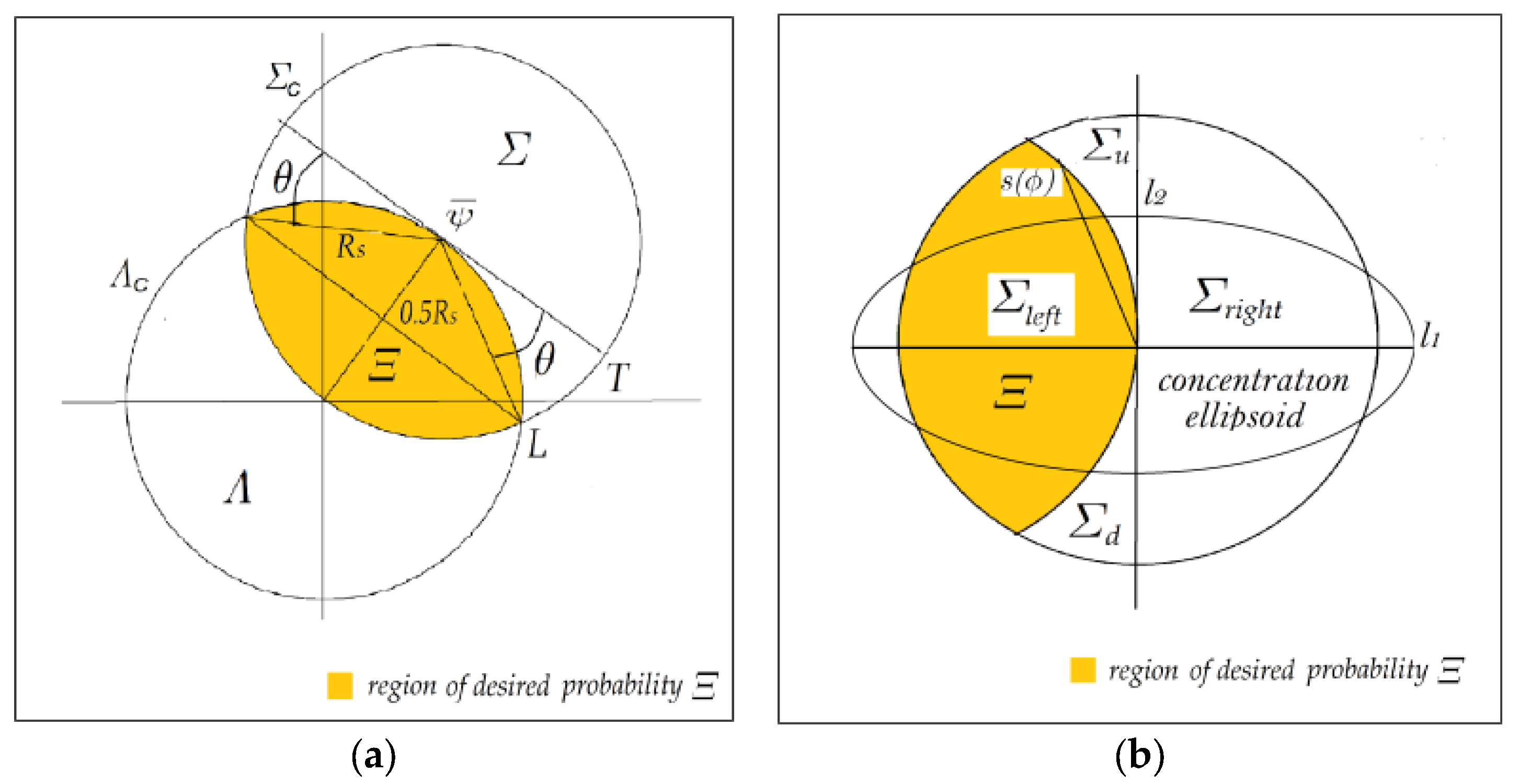
Figure 2.
Identification probability in the CUD.
Table 1.
Simulation results on performance of versus .
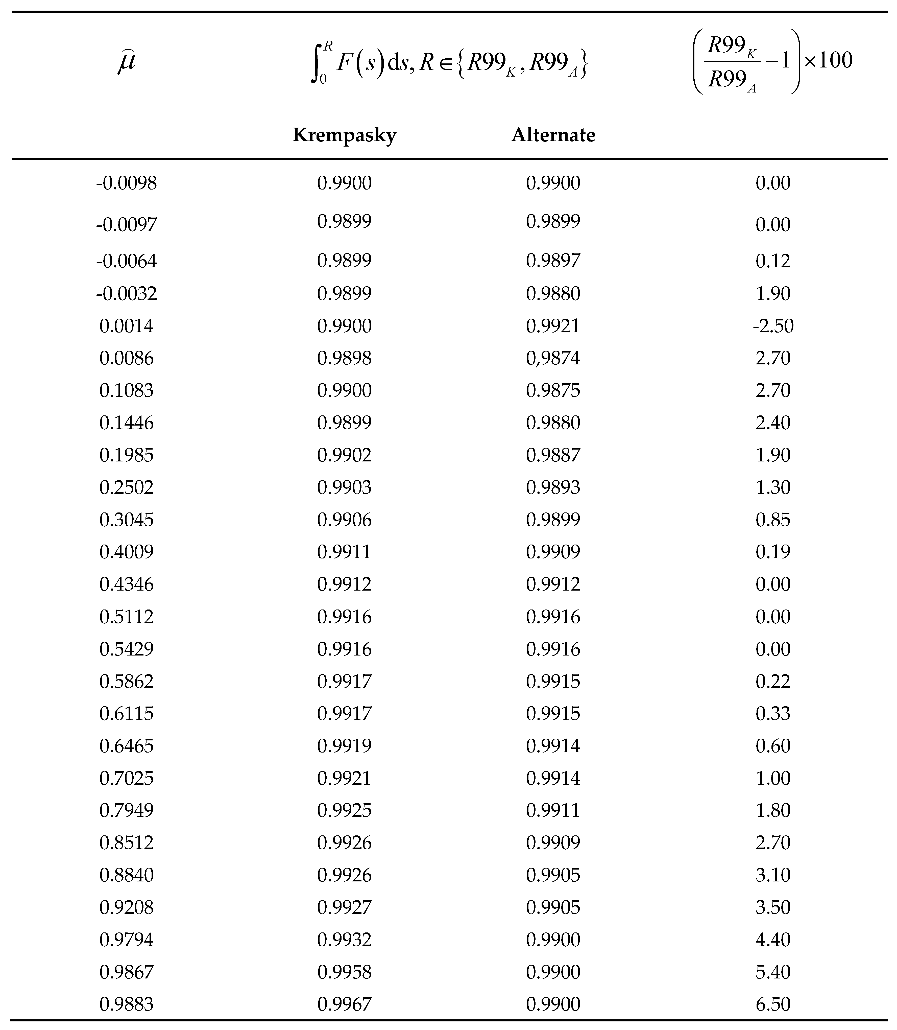
Table 3.
Identification in the CUD.
Disclaimer/Publisher’s Note: The statements, opinions and data contained in all publications are solely those of the individual author(s) and contributor(s) and not of MDPI and/or the editor(s). MDPI and/or the editor(s) disclaim responsibility for any injury to people or property resulting from any ideas, methods, instructions or products referred to in the content. |
© 2024 by the authors. Licensee MDPI, Basel, Switzerland. This article is an open access article distributed under the terms and conditions of the Creative Commons Attribution (CC BY) license (http://creativecommons.org/licenses/by/4.0/).
Copyright: This open access article is published under a Creative Commons CC BY 4.0 license, which permit the free download, distribution, and reuse, provided that the author and preprint are cited in any reuse.


