

Submitted:
18 April 2024
Posted:
19 April 2024
You are already at the latest version
Abstract
Electricity load forecasting is a crucial undertaking within all the deregulated markets globally. In contemporary times, the transition from conventional electricity grids to Smart Grids constitutes an area where extensive research is conducted on a global scale. Among the research challenges, the investigation of Deep Transfer Learning (DTL) in the field of electricity load forecasting represents a fundamental effort that imparts generality to Artificial Intelligence applications, due to new capabilities, such as knowledge transfer and computational power reduction. In this paper a comprehensive study is conducted for day-ahead electricity load forecasting. For this purpose, three Sequence-to-Sequence (Seq2seq) Deep Learning (DL) models are used, namely the Multilayer Perceptron (MLP), the Convolutional Neural Network (CNN) and the Ensemble Learning Model (ELM), which is consisted of the weighted combination of the outputs of MLP and CNN models. Also, the study focuses on the development of different forecasting strategies based on DTL and emphasizing the way the datasets are trained and fine-tuning for higher forecasting accuracy. In order to implement the forecasting strategies using Deep Learning models, load datasets from three Greek islands, Rhodes, Lesvos, and Chios, are used. The main purpose is to apply DTL for day-ahead predictions (1-24 hours) for each month of the year for Chios dataset after training and fine-tuning the models using the datasets of the three islands in various combinations. After several trials, four DTL strategies are illustrated. In the first strategy (DTL Case 1), each of the three DL models is trained using only Lesvos dataset, while fine-tuning is performed on the dataset of Chios island, in order to create day-ahead predictions for Chios load. In the second strategy (DTL Case 2), data from both Lesvos and Rhodes concurrently are used for the DL model training period, and fine-tuning is performed on the data from Chios. The third DTL strategy (DTL Case 3) contains the training of the DL models using Lesvos dataset, and the testing period performed directly on the Chios dataset without fine-tuning. The fourth strategy is a Multi-task Deep Learning (MTDL) approach, which has been extensively studied in recent years. In MTDL, the three DL models are trained simultaneously on all three datasets and the final predictions are made on the unknown part of the dataset of Chios. In this paper, we explore the performance of DTL and compare the results with those produced with MTDL. The results demonstrated that DTL can be applied with high efficiency for day-ahead load forecasting. Specifically, the two cases with fine-tuning (DTL Case 1 and 2) outperformed MTDL in terms of load prediction accuracy. Regarding the DL models, all three exhibit very high prediction accuracy, especially in the two cases with fine-tuning. The ELM excels compared to the single models. More specifically, for conducting day-ahead predictions, it has been concluded that the MLP model presents best monthly forecasts with a MAPE of 6.24% and 6.01% for the first two cases, the CNN model presents best monthly forecasts with a MAPE of 5.57% and 5.60% respectively and the ELM model achieves best monthly forecasts with a MAPE of 5.29% and 5.31%, respectively, indicating the very high accuracy it can achieve.
Keywords:
Deep Transfer Learning
; Electricity Load Forecasting
; Multilayer Perceptron
; Convolutional Neural Network
; Ensemble Deep Learning
; Multi-task Deep Learning
; Exploratory Data Analysis
1. Introduction
Research interest in the electricity sector has been growing because of a few key reasons. First, there’s a global shift toward using sustainable and renewable energy sources like solar and wind. This shift has led researchers to find ways to better incorporate these technologies into existing power grids. Second, the increasing need for electricity due to population growth and industrialization requires new and efficient solutions for transmission, distribution, and consumption of electricity. Third, the development of smart grids and improvements in energy storage technologies has opened up opportunities to enhance the resilience, reliability, and responsiveness of power grids. Additionally, concerns about the environment and climate change have motivated researchers to explore cleaner and more eco-friendly energy options. The digitization of the electricity sector, thanks to advancements in data analytics, machine learning, and Internet of Things (IoT) technologies, has also spurred research into creating smarter and more efficient energy systems. Overall, these factors have created a dynamic landscape, prompting researchers to explore new approaches and technologies to tackle the changing challenges and opportunities in the electricity sector.
Deep Transfer Learning (DTL) refers to the use of Deep Neural Networks (DNNs) in the domain of Transfer Learning. DTL utilizes the knowledge learned from one task to improve the performance of another related task. Usually, in DTL a pre-trained DNN model is fine-tuned for a different task. This domain enhances data efficiency, reduces training time, and enables models to generalize well, capturing underlying patterns in electricity consumption. The ability to adapt to dynamic conditions and the improved accuracy stemming from pre-trained models make transfer learning a valuable tool for addressing the challenges of forecasting in the energy sector. With limited and heterogeneous datasets, transfer learning enables models trained in one domain to be adapted to another, addressing the challenges of varying temporal scales and spatial characteristics. This approach proves essential in optimizing electricity forecasting models, particularly in the face of emerging technologies, changing infrastructures, and the need for resource-efficient solutions. By reusing pre-trained models and enhancing adaptability, transfer learning contributes significantly to robust and accurate predictions, ultimately supporting more effective energy management in the dynamically evolving landscape of the electricity sector.
More generally, in recent years, Transfer Learning is gathering increasing scientific interest. For this purpose, an extensive literature review follows, aiming to present the most comprehensive papers that investigate the specific field. Meng et al. in [1] propose a transfer learning based method for abnormal electricity consumption detection, where a pre-trained model is fine-tuned using a small amount of data from the target domain. Antoniadis et al in [2] discuss the use of transfer learning techniques for electricity load forecasting, specifically in the context of leveraging information from finer scales to improve forecasts at wider scales. Yang et al. in [3] discuss the implementation of a transfer learning strategy to address the multi-parameter coupling problem in the design of water flow enabled generators. Dong et. al. in [4] propose a transfer learning model based on Xception neural network for electrical load prediction, which is trained using pre-trained models and fine-tuned in the training process. Li et al. in [5] explore a transfer learning scheme for non-intrusive load monitoring (NILM) in smart buildings, which involves transferring a well-trained model to estimate power consumption in another data set for all appliances. Peirelinck et al. in [6] discuss the use of transfer learning techniques in the context of demand response in the electricity sector. It shows that transfer learning can improve performance by over 30% in various tasks. Laitsos et al. in [7] use Transfer Learning Technique with several Deep Learning models to predict energy consumption of Greek Islands and the pre-trained model demonstrates outstanding flexibility when adapting to a new and unknown dataset. Wu et al. in [8] propose an attentive transfer framework for efficient residential electric load forecasting using transfer learning and graph neural networks. Syed et al. in [9] propose a reliable inductive transfer learning (ITL) method for load forecasting in electrical networks, which uses knowledge from existing deep learning models to develop accurate ITL models at other distribution nodes. Laitsos et al. in [10] propose an automated Deep Learning application for electricity load forecasting. Santos et al. in [11] propose a novel methodology that combines transfer learning and deep learning techniques to enhance short-term load forecasting for buildings with limited electricity data. Arvanitidis et al. in [12] propose clustering MLP models for short-term load forecasting. Luo et al. in [13] discuss the use of transfer learning techniques for load, solar, and wind power predictions, but it does not specifically mention the application of transfer learning to load prediction. Li et al. in [14] discuss a short-term load forecasting framework that adopts Transfer Learning. Transfer learning is used to train learnable parameters based on trend components and then transfer them to the load forecasting model. Chan et al. in [15] introduce a hybridized modelling approach, using a Convolutional Neural Network (CNN) and a Support Vector Machine (SVM), for short-term load forecasting. Kontogiannis et al. in [16] propose a structural ensemble regression algorithm for cluster-based aggregate electricity demand forecasting.
Jung et al. in [17] propose an electricity load forecasting framework on a monthly basis for smart cities, using transfer learning techniques. It collects data from multiple districts, selects similar data based on correlation coefficients, and fine-tunes the model using target data. Al-Hajj et al. in [18] is a survey of transfer learning in renewable energy systems, specifically in solar and wind power forecasting, load prediction, and fault diagnosis. Nivarthi et al. in [19] discuss the use of transfer learning in renewable energy systems, specifically in power forecasting and anomaly detection. It proposes a transfer learning framework and a feature embedding approach to handle missing sensor data. Miraftabzadeh et al. in [20] present a framework based on transfer learning and deep neural networks for day-ahead photovoltaic power prediction. Vontzos et al. in [21] propose a data-driven short-term forecasting for electricity consumption in airport. Yang et al. in [22] propose an innovative monthly DNN approach, for load forecasting in urban and regional areas. In order to draw more secure conclusions, an extended comparison with other Machine Learning models is conducted. Li et al. in [23] propose a building electricity load forecasting method based on Maximum Mean Discrepancy (MMD) and an improved TrAdaBoost algorithm (iTrAdaBoost).
The relentless growth of electricity demand, coupled with the dynamic and often unpredictable nature of energy consumption patterns, necessitates advanced forecasting methods for effective grid management. In this context, transfer learning emerges as a promising paradigm to address the challenges associated with limited and disparate data sources. This research paper delves into the application of deep transfer learning techniques in the domain of electricity forecasting, aiming to exploit knowledge gained from one source domain to improve predictive accuracy in a target domain. By leveraging pre-existing models trained on related datasets or domains, transfer learning seeks to enhance the adaptability and robustness of forecasting models, ultimately contributing to more accurate and reliable predictions in the complex and ever-evolving landscape of electricity demand. This paper explores the theoretical foundations, methodologies, and practical implications of transfer learning in the specific context of electricity forecasting, shedding light on its potential to revolutionize the field and pave the way for more resilient and efficient energy management systems.
With respect to the contribution of this paper, the following points are emphasized:
- For the first time, a high accuracy results implementation of Sequence to Sequence (Seq2seq) Ensemble Deep Transfer Learning for day-ahead (1-24 hours) forecasting is conducted on three distinct datasets from islands of the Greek power system. Although the training dataset of Rhodes exhibits somehow different behavior, compared to the other two datasets, the proposed algorithms perform very satisfactory results. This fact further enhances the performance of the proposed strategies and models. The characteristics of the Rhodes dataset lead to a more robust and comprehensive evaluation of the models, as it introduces variability and challenges that may not be present in the other datasets. This diversity in behavior across datasets provides a more realistic and thorough assessment of the models’ capabilities.
- The results obtained indicate that Deep Transfer Learning (DTL) could provide particular value to both Transmission System Operators (TSO) and Distribution System Operators (DSO), within various regions of the Greek system.
- The application of the models is performed on actual load data with minimal data preprocessing, a fact that creates optimistic conclusions regarding their applicability under real-time conditions.
This paper is organized as follows: First, at Section 2, the Exploratory Dataset Analysis and the Feature Creation is employed. After, at Section 3 the forecasting strategies are analyzed. At Section 4, the emerged results for every algorithm along with the discussion about their performance are presented. Finally, at Section 5, the main conclusions and future study proposals are analyzed.
2. Materials and Methods
2.1. Dataset Analysis
In this section, all features, behaviors, and correlations of the three datasets used are investigated and analyzed. Initially, the three timeseries under study are presented, and then emphasis is given to their monthly and daily average fluctuations.
Figure 1 illustrates the three power timeseries fluctuations for each of the three datasets in hourly resolution. What is noteworthy is that Rhodes, especially during the summer months, experiences a substantial increase in demand. The other two islands exhibit several similarities between them, with both the average and extreme values behaving relatively similarly. This consistency in behavior across the two datasets suggests common characteristics or patterns in the energy-related dynamics of these islands. The shared trends in both average and extreme values contribute to a more coherent and comparable analysis between the two datasets, aiding in the development and assessment of models for these specific island environments.
Figure 2 presents the monthly boxplots for each of the three datasets.
Also, Figure 3 visualizes the average daily electricity consumption (1-24 hours) for each island.
This Figure clearly illustrates that the average hourly values for Rhodes are significantly higher than those of the other two islands. However, it is noteworthy that the three patterns exhibit high similarities among them, a fact demonstrated by common peak and off-peak demand hours among the three islands.
2.2. Data Preprocessing
In order to shape the raw data into a suitable format, capable of being used as inputs in Deep Learning models, the preprocess involves the following four stages:
- Anomaly Detection: Anomaly detection in timeseries involves establishing a baseline of normal behavior through statistical methods or machine learning algorithms, extracting relevant features, and training a model on labeled data to distinguish normal patterns from anomalies. Due to instances of zero consumption during specific hours, likely caused by network faults, these particular values were set equal to the corresponding values from one week prior. This adjustment was made to address the challenge of unexpected situations in the data, as algorithms may struggle to account for such anomalies. The goal is to ensure the optimal training of each model by handling these irregularities in the dataset.
- Filling missing values: Filling missing values in timeseries data is a crucial preprocessing step for anomaly detection. Since anomalies are often identified based on patterns and trends in the data, it’s essential to address gaps caused by missing values.
- Min-Max Scaling: This preprocessing method applied to all datasets in this paper involves Min-Max Scaling, which normalizes data points to a range between 0 and 1. To achieve this, two distinct scalers were employed—one for input and another for output datasets. The primary rationale behind utilizing Min-Max Scaling is its ability to enhance the efficiency of training deep learning models during the training phase, facilitating faster convergence to the optimal solution of the loss function.
- One-Hot Encoding: With this process, numerical data are transformed to cyclical, through trigonometric equations. In this study, day of the week, hour of the day and month of the year were converted to sin and cosine formulation. Figure 4 represents the day of the week transformed in sin and cosine format.
2.3. Feature Creation
In this subsection, the parameters used as inputs for the models are being generated. For this reason, several input features were studied and evaluated in order to understand the most significant for predicting electricity demand. Eight input features were investigated for forecasting day-ahead electricity demand. The input variables used for all Deep Learning Models remain consistent and are presented in detail below.
- Power in hourly resolution: The sequence of 168 hours of load values for 7 days/one week.
- Cos of Day of Week: The sequence of 168 values of Day of the Week (0-6) converted by One Hot Encoding to cosine type.
- Sin of Day of Week: The sequence of 168 values of Day of the Week (0-6) converted by One Hot Encoding to sin type.
- Cos of Hour of Day: The sequence of 168 values of Hour of Day (0-23), converted by One Hot Encoding to cosine type.
- Sin of Hour of Day: The sequence of 168 values of Hour of Day (0-23), converted by One Hot Encoding to sin type.
- Cos of Month of Year: The sequence of 168 values of Month of the Year (1-12) converted by One- Hot Encoding to cosine type.
- Sin of Month of Year: The sequence of 168 values of Month of the Year (1-12) converted by One- Hot Encoding to sin type.
- IsWeekend: The sequence of 168 values of a dummy variable named “Is Weekend”, with value equal to 0 for working days and 1 for weekends and holidays.
Our target is to utilize a historical sequence of 168 hours from the aforementioned 8 features, and create day-ahead predictions for the load, i.e., a sequence of 24 values of the Power. Figure 5 visualizes the Seq2seq prediction technique.
Finally, the correlation heatmap is presented in Figure 6, in order to highlight the relationships between the power timeseries for each of the three islands.
What is noteworthy is that the target timeseries of Chios shows a correlation of 0.37 with that of Rhodes and 0.94 with that of Lesvos. This particular characteristic further enhances the reliability of the implemented applications, demonstrating generality and robustness through the results that will be presented below. The correlation between the target timeseries of different islands suggests some level of interdependence or shared patterns, which can contribute to the generalization and effectiveness of the models developed for these islands.
3. Methodology
In this section, the fundamental methodology followed in the paper is presented. Initially, an introduction of the three DL models is presented. Then, the forecasting strategies are analyzed in depth, emphasizing all the details of each one, highlighting the way datasets are utilized for each strategy. Subsequently, a reference is made to the Optimization framework, which has been used for enhancing the performance of the DL models. Additionally, the evaluation metrics are presented, which were used to evaluate and compare the performance of the algorithms of each strategy. Finally, the software tools that were used are analyzed.
3.1. Deep Learning Models
In this subsection, the functionality and architectures of the three DL models used in the paper, MLP, CNN, and ELM, are analyzed.
3.1.1. Multilayer Perceptron
A Multilayer Perceptron (MLP), which is presented in Figure 7, is a versatile artificial neural network architecture employed for learning and modeling complex relationships within data. Comprising an input layer (X), one or more hidden layers (), and an output layer (Y), the MLP is characterized by its capacity to capture intricate non-linear patterns. During forward propagation, the input data is transformed through weighted connections and activation functions () in the hidden layers, generating progressively abstract representations. The hidden layer outputs () can be mathematically expressed as:
where denotes the weight matrix connecting layer to i, is the output of the previous layer, and represents the bias term for layer i. The activation function introduces non-linearity, enabling the network to capture complex mappings.
The final output (Y) is computed through similar operations in the output layer:
During training, the network adjusts its weights to minimize a defined loss function (L), which quantifies the disparity between the predicted output and actual target values. The weights are updated using an optimization algorithm, typically gradient descent, with the weight update rule expressed as:
where is the learning rate. This iterative process, known as back propagation, refines the model’s weights to improve its predictive accuracy.
In the domain of timeseries forecasting, MLPs exhibit efficiency owing to their inherent ability to capture temporal dependencies and non-linear patterns. The adaptability of the model enables it to discern and model various temporal structures, including trends and seasonality. The hidden layers serve as dynamic feature extractors, automatically learning relevant temporal features from the timeseries data. This feature learning capability, coupled with the tunability of model parameters, positions MLPs as robust and effective tools for a wide array of timeseries forecasting tasks.
3.1.2. Convolutional Neural Network
Convolutional Neural Networks (CNNs), the architecture of which is presented in Figure 8, constitute a class of sophisticated deep learning architectures specifically designed for the analysis and processing of visual data. The principal structure of CNNs encompasses multiple layers, notably including convolutional layers, pooling layers, and fully connected layers. Convolutional layers assume a pivotal role in feature extraction from input images through the application of convolutional operations utilizing trainable filters. These filters adeptly identify patterns and features at various spatial scales, enabling the network to discern intricate details within the data. Accompanying pooling layers serve to diminish the spatial dimensions of feature maps, thereby diminishing computational complexity and augmenting the model’s capacity for generalization. The culmination of these operations transpires in fully connected layers positioned at the conclusion of the network, where the amalgamated features facilitate conclusive predictions. The applicability of CNNs extends across diverse computer vision domains, manifesting notable success in tasks such as image classification, object detection, and image segmentation.
In timeseries forecasting, CNNs adapt to sequential data using 1D convolutional layers. These layers analyze temporal patterns, aided by pooling layers for downsizing. CNNs efficiently capture short and long-term dependencies, making them valuable for tasks such as stock price prediction and weather forecasting, showcasing their versatility across diverse data types.
3.1.3. Ensemble Learning Model
The Ensemble Learning Model (ELM), comprising a Multilayer Perceptron (MLP) and a Convolutional Neural Network (CNN), operates by independently training both models on a given dataset and then combining their predictions through weighted averaging. The MLP focuses on learning non-linear relationships, while the CNN excels at extracting hierarchical features. The weights assigned to each model in the ensemble are determined based on their performance, enhancing the contribution of the better-performing model. The final prediction is generated by summing the weighted predictions, aiming to capitalize on the complementary strengths of the MLP and CNN for improved predictive accuracy and robustness across diverse data patterns. Figure 9 visualizes the main body of ELM created in this paper.
3.2. Deep Transfer Learning Forecasting Strategies
The first forecasting strategy, named Deep Transfer Learning Case 1 (DTL Case 1), involves training each of the three DL models exclusively on the Lesvos dataset, with fine-tuning carried out using the Chios dataset. In the second strategy, Deep Transfer Learning Case 2 (DTL Case 2), both Lesvos and Rhodes datasets are used concurrently during the DL model training phase, followed by fine-tuning using the Chios dataset. The third strategy, Deep Transfer Learning Case 3 (DTL Case 3), entails training the DL models solely on the Lesvos dataset, with the testing phase conducted directly on the Chios dataset, without any fine-tuning. Lastly, in the Multi-task Deep Learning application strategy (MTDL), each of the three DL models are trained simultaneously on all three datasets, with final predictions made on the unused portion of the Chios dataset.
The way in which the available data were used in order to implement the DTL strategies and the MTDL strategy is described below:
- For DTL Case 1, only the dataset of Lesvos was used for the first training phase of the models, specifically for the time period from 2019-01-01 01:00:00 to 2021-12-31 23:00:00. Then, for the second phase, i.e., fine-tuning, the time period from 2019-01-01 01:00:00 to 2021-12-31 23:00:00 of the Chios dataset is utilized.
- For DTL Case 2, the first training phase of the models was based on the datasets from Lesvos and Rhodes, and more specifically, for the time period from 2019-01-01 01:00:00 to 2021-12-31 23:00:00 for each dataset. Then, for the second phase, i.e., fine-tuning, the same time period as in DTL Case 1 is used, from 2019-01-01 01:00:00 to 2021-12-31 23:00:00 of the Chios dataset.
- For DTL Case 3, the training dataset that was used covers the time period from 2019-01-01 01:00:00 to 2022-12-31 23:00:00 from the Lesvos dataset without fine tuning. The choice of Lesvos alone was made because it exhibits a higher correlation and similarity with the corresponding dataset of the Chios timeseries, compared to the Rhodes island.
- For MTDL, the datasets from all three islands were used simultaneously for training. Specifically, the datasets of Rhodes and Lesvos for the time period 2019-01-01 01:00:00 to 2022-12-31 23:00:00, and for Chios dataset, for the time period 2019-01-01 01:00:00 to 2021-12-31 23:00:00 were used.
Deep Transfer Learning is a field of Transfer Learning that entails utilizing knowledge gained from solving one task to make predictions on another related task, employed Deep Neural Networks. This field often consists of pre-training a neural network on a source task with abundant labeled data and subsequently applying the acquired knowledge to a target task characterized by a foreign dataset. Two prevalent scenarios in transfer learning include domain adaptation, where the source and target tasks have the same input space but differ in output spaces, and feature extraction, where the source and target tasks share similar input and output spaces.
In the realm of timeseries approaches, is valuable for several reasons. Timeseries data often exhibits complex patterns, trends, and seasonality, and acquiring labeled data for training deep models can be challenging due to limited availability. It allows a model pre-trained on a source timeseries task to capture generic temporal features and representations that can be beneficial for a target task. The learned features can serve as a useful initialization for the target task, reducing the need for extensive training data and potentially enhancing the model’s ability to generalize to new patterns. Additionally, transfer learning is particularly advantageous when the source and target tasks share similar temporal characteristics, enabling the model to transfer knowledge effectively and improve its performance on the target task. This approach is especially relevant in situations where collecting large amounts of labeled data for every specific task is impractical or costly.
In this paper, DTL strategies with and without fine-tuning are developed. Initially, the two cases of DTL with fine-tuning are examined (DTL Case 1 and 2) and are analyzed below. Subsequently, the scenario where the pre-trained model, as configured without fine-tuning, is examined (DTL Case 3). Finally, the MTDL strategy, involving the simultaneous training of each DL model on the datasets of the three islands, is presented. The four proposed forecasting strategies implemented are analyzed and presented in detail below.
3.2.1. Deep Transfer Learning Case 1
In this methodology a DNN pre-trained on a source task is adjusted to perform a related target task. Initially trained on a large dataset for a general task, such as laod forecasting, the pre-trained model captures broad features. This knowledge is then transferred to a target task, which is a foreign dataset. During fine-tuning, the model’s weights, especially in the deeper layers, are adjusted based on the target task’s data, allowing the model to adapt its learned representations to task-specific characteristics. This approach is particularly advantageous when the target task has also limited labeled data, enabling the model to leverage the knowledge gained from the source task and enhance its performance on the target task.
In DTL Case 1, the testing dataset of Chios is used, and the training dataset consists only of the timeseries of Lesvos island. This approach is followed due to higher correlation between Chios and Lesvos compared to Rhodes, influencing the selection of training data for better model performance. After, the training period, fine-tuning is performed on the training parts of each model on the dataset of Chios, creating the final fine-tuned models. Finally, these models are used for Chios day-ahead load forecasting. Graphically, Figure 11 visualizes the DTL Case 1 strategy.
3.2.2. Deep Transfer Learning Case 2
Similarly with DTL Case 1, for DTL Case 2, the two datasets from Rhodes and Lesvos are merged, and the three models are trained on the combined training dataset. The trainable part of the pre-trained model is fine-tuned in the dataset of Chios. Finally, the predictions are made on the unused dataset from Chios island. Figure 11 visualizes this strategy.
3.2.3. Deep Transfer Learning Case 3
Deep Transfer learning without fine-tuning involves a two-step process. Initially, a Deep Neural Network is trained on a source task using a substantial dataset, learning hierarchical features relevant to that task. Subsequently, in the transfer phase, the pre-trained model is utilized with the exact same structure as it was formed during the training period, in order to create predictions for a target task. The learned features are extracted without further adjusting the model’s weights, and these fixed representations serve as input to a new task-specific regressor trained on the target task’s dataset.
This approach proves advantageous when the target task possesses limited labeled data, as it allows for knowledge transfer from a source task without the computational overhead of fine-tuning the entire model. By utilizing the pre-trained model as a feature extractor, the knowledge encapsulated in the generic representations can be harnessed for tasks that share similar low-level features and structures, promoting effective knowledge transfer across related tasks while mitigating the need for task-specific fine-tuning.
In DTL Case 3 strategy, the three DL models are trained on the dataset of Lesvos, and subsequently, predictions are made directly on the Chios day-ahead load, without fine-tuning process. This strategy is used in order to draw secure conclusions regarding the approaches with and without fine-tuning. This strategy is presented in Figure 12.
3.2.4. Multi-Task Deep Learning
Multi-task Deep Learning (MTDL) is a Multi-task Learning (MTL) methodology in Deep Neural Networks (DNN), where a DNN model is trained simultaneously on multiple datasets, leveraging the shared knowledge across the different datasets to improve the model’s generalization performance. The underlying principle of MTDL is to exploit the relationships and commonalities among distinct but related tasks, allowing the model to learn a shared representation that captures the inherent structure present in the data. Essentially, a unified dataset is created, which is a concatenation of different datasets, where each of them corresponds to a specific output. During training, the model optimizes its parameters by jointly minimizing the loss across all tasks. The shared representation learned across tasks facilitates the transfer of knowledge between them, leading to enhanced generalization performance, particularly in scenarios where individual tasks lack sufficient data for robust learning. The success of MTDL lies in its ability to induce a form of regularization, encouraging the model to discover and focus on relevant features that are beneficial for multiple tasks simultaneously.
Each of the training task has its own objective function, and the model learns to jointly optimize these objective functions. The general idea is to share information across tasks to improve overall performance. Mathematically, the following applies:
- N is the total number of tasks.
- X are the input data.
- is the output for task i.
- are the parameters of the neural network model.
For each task i, there is an associated loss function that measures the error between the predicted output and the true output for that task. The overall loss function for all tasks can be defined as a combination of the individual task loss functions, often using a weighted sum:
where are optional weighting factors and represents the loss for the task.
The goal is to minimize this overall loss function with respect to the model parameters . The minimal value of the loss function, , is given below:
The model parameters are then updated using gradient descent or other optimization techniques to minimize this combined loss. The shared representation in the intermediate layers allows the model to discover commonalities and relationships among tasks, promoting a more generalized feature extraction process. By training on diverse datasets simultaneously, MDTL facilitates the development of a model that not only excels in individual tasks but also demonstrates improved performance on new, foreign data.
In the strategy employed in this paper, which is presented in Figure 13, training is conducted simultaneously on all three different datasets of the islands, Rhodes, Chios and Lesvos. The objective is for the model to acquire high generalization capabilities and make predictions on the testing dataset selected of Chios. Due to the distinct variations in the three timeseries, this approach proves more robust than cases involving singular training, imparting generality in performance across the models.
3.3. Optimization Framework
The Bayesian Optimization Algorithm (BOA) is utilized for each training period and for each model. It is a probabilistic optimization approach designed to tackle complex and computationally expensive objective functions. Central to BOA is the use of a surrogate model, typically a Gaussian Process, which provides a probabilistic representation of the unknown objective function. This surrogate model captures both the mean and uncertainty associated with the objective function across the parameter space. The algorithm iteratively refines its understanding of the objective function by selecting points for evaluation based on an acquisition function that balances exploration and exploitation. The chosen points are then used to update the surrogate model through Bayesian inference, adjusting the model’s predictions in light of the new information. This iterative process allows BOA to systematically explore the parameter space, adapt to the underlying structure of the objective function, and efficiently converge towards optimal solutions.
BOA excels in making informed decisions by using the uncertainty measured by its surrogate model. An acquisition function guides the algorithm to explore areas where the objective function is uncertain or likely to have optimal values. As the optimization progresses, the surrogate model of BOA improves continuously, enhancing its understanding of the objective function and focusing the search on regions most likely to contain the global optimum. This principled approach makes it particularly well-suited for optimization problems in scientific and engineering domains where objective function evaluations are resource-intensive or subject to noise. It efficiently identifies optimal parameter configurations in such scenarios.
3.4. Evaluation Metrics
For this paper, the following four error prediction metrics are used.
Mean Absolute Error (MAE): In this metric, the average of the absolute differences between the forecasted and true values is calculated.
Root Mean Squared Error (RMSE): This metric calculates the square root of the average of the squared differences between the forecasted and true values.
Mean Absolute Percentage Error (MAPE): This metric computes the average of the absolute percentage differences between the predicted and actual values.
R-squared (): Is a statistical metric that measures how the independent variable(s) in a forecasting model explain the variation of the dependent variable. It takes values between 0 and 1. 1 belongs to a satisfactory fit, meaning all variation in the dependent variable is explained by the independent variable(s). 0 demonstrates zero connection between the variables.
The above metrics are defined as follows:
where , and are the forecasting, the actual, the mean of the forecasting values and the mean of the actual values, respectively.
3.5. Software environment
All the algorithms of this work developed using the Python 3.10 programming language. The open-source software library Tensorflow 2.15.0 and the high-level API Keras 2.15.0 were employed for training and testing the deep learning algorithms. Additionally, Pandas 2.1.0 and Numpy 1.26.0 libraries were utilized for data analysis. For visualization purposes in exploratory analysis and prediction results, the Seaborn, Plotly, Matplotlib, graphviz and torchviz libraries were incorporated. Also, the official Calendar library was used, in order to identify the weekends and the Greek holidays. The research was conducted on the Google Colab Pro environment. For the MLP model the GPU Tesla T4 with specific characteristics: NVIDIA-SMI 535.104.05 Driver Version: 535.104.05 CUDA Version: 12.2, RAM: 12.7 GB, and disk space: 78.2 GB was used. For the CNN and Ensemble model a cloud TPU 28.6 GB RAM abd 107.7 GB disc space was employed.
4. Results Analysis
In this section the experimental results obtained are presented. First, only the mean variance of the Mean Absolute Error (MAE) on a monthly basis for the MLP, CNN and ELM, respectively, is presented, for the economy of space. Then, MAPE (Mean Absolute Percentage Error), RMSE (Root Mean Square Error) and the aggregated results are visualized, analyzed and compared for each strategy and each model, on a monthly basis. Finally, the Tables detailing are presented in the aggregated results.
4.1. Multilayer Perceptron Results
Figure 14 visualizes the variation of MAE, on a monthly basis, for each of the four strategies, for MLP model. It is observed that May and September exhibit better prediction results, while January, July, and August are the months with poorer performance.
4.2. Convolutional Neural Networks Results
Figure 15 presents the variation of MAE, on a monthly basis, for each of the four strategies, for CNN. It is clearly seems that April and May exhibit better average prediction results, while June, July, and August are the months with the worst performance.
4.3. Ensemble Learning Model Results
Figure 16 visualizes the variation of MAE, on a monthly basis, for each of the four strategies, for the Ensemble Learning model. It is observed that June, July and August exhibit better average prediction results, while May, September, and October are the months with the lowest prediction accuracy.
4.4. Results Comparison
In order to make an evaluation of the performance of each model, the results are consolidated and comparatively analyzed for each of the four strategies that were pursued in the following radial graph. This particular graph was chosen because it constitutes an illustrated and clear approach in presenting results for each of the twelve months of the year. To elaborate, the closer a point is to the center of the circle, the lower the prediction error achieved.
4.4.1. Variation of MAE for Each Strategy
Figure 17 presents the comparison month by month of Mean Absolute Error (MAE) of the DL models for each strategy.
Based on the comparative results, the following observations emerge:
- For the DTL strategy with fine-tuning and training data from the Lesvos timeseries, DTL Case 1, it is observed that the MLP and Ensemble models outperform the CNN model.
- In the forecasting strategy with fine-tuning and training data from both the Rhodes and Lesvos timeseries, DTL Case 2, it seems that the MLP and Ensemble models exhibit comparable performance, except for October, where MLP outperforms.
- Regarding for the use of pre-trained models without fine-tuning, DTL Case 3, the CNN significantly lags behind the other two models, with MLP consistently exhibiting the highest prediction accuracy.
- Finally, regarding the Multi-task Deep Learning application strategy, MTDL, it is observed that the MLP model consistently shows inferior results compared to the other two models for all months. Here, the CNN and Ensemble achieve similar accuracy.
For additional analysis and understanding of the behavior of the algorithms, Figure plot the variation of the Mean Absolute Percentage Error (MAPE) and Root Mean Squared Error (RMSE) for each month.
4.4.2. Variation of MAPE for Each Strategy
Figure 18 presents the comparison of Mean Absolute Percentage Error (MAPE) for each model and strategy, on a monthly basis.
It is clearly observed that for the DTL Cases 1 and 2, June exhibits the best prediction accuracy, with the Ensemble model achieving a MAPE of 5.29% for Case 1 and the MLP achieving a MAPE of 6.01% for Case 2. In the case of MTDL, the best predictions are observed in the months of June and July, with the ELM presenting predictions of 6.33% and 6.86%, respectively. Finally, for the DTL Case 3, the best prediction is observed in January, corresponding to a MAPE of 7.85%, achieved by the ELM model.
4.4.3. Variation of RMSE for Each Strategy
Figure 19 presents the comparison of Root Mean Squared Error (RMSE) for each model and strategy, on a monthly basis.
4.5. Aggregated Results
This subsection provides a detailed presentation of the results obtained for each forecasting strategy and each DL model, on a monthly basis. Table 1, Table 2, Table 4, and Table 3 present all the aggregated results for each forecasting strategy, aiming to provide a complete view of the performance of each algorithm and for each forecasting month. MAE and RMSE metrics are given in MWs, MAPE is given in percent (%), and takes values between 0-1.
Based on the results of Tables, the following summarizations apply:
- In DTL Case 1, it is observed that the Ensemble model achieves the best prediction for the month of June, presenting an MAPE of 5.29%.
- In DTL Case 2, again, the Ensemble model achieves the best prediction, which pertains to the month of February and exhibits an MAPE of 5.31%.
- Regarding the DTL Case 3, the Ensemble model achieves the best prediction in January with an MAPE of 7.85%.
- In MTDL, the CNN model manages the best prediction in January, corresponding to an MAPE of 5.62%.
4.6. Results Discussion
Based on the above results, it becomes evident that the application of Deep Learning algorithms in the domain of Deep Transfer Learning (DTL) can yield satisfactory outcomes, reducing computational power requirements and model training times, due to the fact that, after the initial training of the model, only the fine-tuning needs to take place each time the DL model is applied in a different area. The time required for a DL model to be trained during the fine-tuning period is significantly shorter compared to the time needed for direct training, as in the case of MTDL. Also, the variation in results for each month indicates that the ELM improves predictions for the majority of forecasted months.
In general, it is observed that the two strategies of Deep Transfer Learning with fine-tuning (DTL Case 1 and 2) significantly outperform DTL Case 3 and MTDL. Specifically, in the comparison between fine-tuning strategies and Multi-task Deep Learning, the differences suggest that the utilized models can adapt better when trained separately on different datasets, as opposed to parallel and simultaneous training on multiple datasets together. Both of these cases involve efforts to create models capable of efficiently generalizing to unknown and differently behaving timeseries.
Additionally, in the case of the direct use of a pre-trained model (DTL Case 3), a poorer performance is achieved compared to other cases. For the ELM, which is influenced by both the MLP and CNN models, the poor performance of the CNN negatively impacts the accuracy for most months, with exceptions in January and July.
The variation in results clearly demonstrates that the employment of more than one model in an ensemble combination, significantly improves the performance compared to individual algorithms. The reason behind this improvement lies in the weighted average learning, which takes into account the best predictions from both models, MLP and CNN separately. As a result, the final day-ahead load prediction is considerably enhanced, showcasing the effectiveness of combining multiple models.
Finally, it is worth noting that the adaptability of the algorithms to the three examined timeseries relies on both the trainable parameters of each model and the different features and patterns exhibited by each case. Seasonality, peak demand periods, and the average values of each dataset are some of the characteristic that influence algorithmic functionalities.
5. Conclusion and Future Study Proposals
In this study, an extensive investigation is conducted regarding Seq2Seq Deep Transfer Learning on timeseries data. For this reason, a case study of a month-to-month approach was employed with the aim of day-ahead forecasting of electricity load in three islands of the Greek power system. The obtained results provided us with important valuable insights regarding the application of such methods and their effectiveness. The first major conclusion is that transfer learning outperforms simple learning, even in the case of Multi-task Deep Learning, which is utilized for better model generalization.
Furthermore, another conclusion is that Deep Transfer Learning using Ensemble models outperforms simple DL models, as evidenced by the results obtained. More specifically, in the strategies DTL Case 1, DTL Case 2, as well as MTDL, it is observed that, for the majority of months, the ELM enhances the predictions achieved by the two individual DL models. This fact creates particularly optimistic conclusions regarding further exploration of Ensemble Models in the field of prediction in power systems.
DTL strategies are cost-effective, requiring significantly less computational power and time compared to simple prediction methods, due to the fact that the DL models are training once in a source dataset, after they are saved in appropriate format, and subsequently only their final part is fine-tuned for each specific task. Therefore, DTL minimizes the computational resources required and speeds up training for a specific target task, like the day-ahead electricity load forecasting. By leveraging the knowledge stored in pre-trained models, DTL efficiently utilizes resources, facilitating swift deployment of effective models across different domains.
In the context of future study proposals, it should be emphasized initially that DTL could be applied to other branches of power systems, such as fault prediction in electric power transmission and distribution networks. Furthermore, beyond energy systems, it could be highlighted that a significant challenge lies in the application of DTL to areas like healthcare, where numerous research studies are conducted globally.
As already mentioned, the study of DTL using ELM, both in the field of power systems and in other domains, can prove capable of further improving the results of Transfer Learning.
Finally, the combination of DTL with Reinforcement Learning holds promise for future research, offering potential advancements. It could be explored to enhance the efficiency of demand forecasting and load management systems. For instance, a pre-trained Reinforcement Learning agent could learn general patterns and behaviors from historical data across different regions or time periods. This pre-trained agent could then be fine-tuned on a specific locality or timeframe, in order to adapt to unique characteristics and changes in electricity demand. This approach may lead to more accurate and adaptable models for load prediction, contributing to improved resource planning and energy efficiency in the electricity grid.
Author Contributions
Conceptualization, V.L. and G.V.; methodology, V.L.; software, V.L. and G.V.; validation, V.L., G.V., A.T., D.B. and L.H.T.; formal analysis, V.L. and G.V.; investigation, V.L. and G.V.; resources, V.L. and G.V.; data curation, V.L. and G.V.; writing—original draft preparation, V.L. and G.V.; writing—review and editing, V.L., G.V., A.T., D.B. and L.H.T.; visualization, V.L. and G.V.; supervision, D.B. and L.H.T.; project administration, D.B. All authors have read and agreed to the published version of the manuscript.
Funding
This research received no external funding.
Data Availability Statement
The load data used in this study are available from the HEDNO portal in [24].
Conflicts of Interest
The authors declare no conflicts of interest.
Abbreviations
The following abbreviations are used in this manuscript:
| BO | Bayesian Optimization |
| CNN | Convolutional Neural Network |
| DNN | Deep Neural Network |
| DTL | Deep Transfer Learning |
| EDA | Exploratory Data Analysis |
| EDL | Ensemble Deep Learning |
| MAE | Mean Absolute Error |
| MAPE | Mean Absolute Percentage Error |
| MDTL | Multi-task Deep Transfer Learning |
| MLP | Multilayer Perceptron |
| R2 | R-Squared |
| RMSE | Root Mean Squared Error |
| Seq2Seq | Sequence-to-Sequence |
References
- Meng, S.; Li, C.; Tian, C.; Peng, W.; Tian, C. Transfer learning based graph convolutional network with self-attention mechanism for abnormal electricity consumption detection. Energy Reports 2023, 9, 5647–5658. [Google Scholar] [CrossRef]
- Antoniadis, A.; Gaucher, S.; Goude, Y. Hierarchical transfer learning with applications to electricity load forecasting. International Journal of Forecasting 2023. [Google Scholar] [CrossRef]
- Yang, C.; Wang, H.; Bai, J.; He, T.; Cheng, H.; Guang, T.; Yao, H.; Qu, L. Transfer learning enhanced water-enabled electricity generation in highly oriented graphene oxide nanochannels. Nature Communications 2022, 13, 6819. [Google Scholar] [CrossRef] [PubMed]
- Dong, Y.; Xiao, L. A Transfer Learning Based Deep Model for Electrical Load Prediction. 2022 IEEE 8th International Conference on Computer and Communications (ICCC), 2022, pp. 2251–2255. [CrossRef]
- Li, D.; Li, J.; Zeng, X.; Stankovic, V.; Stankovic, L.; Xiao, C.; Shi, Q. Transfer learning for multi-objective non-intrusive load monitoring in smart building. Applied Energy 2023, 329, 120223. [Google Scholar] [CrossRef]
- Peirelinck, T.; Kazmi, H.; Mbuwir, B.V.; Hermans, C.; Spiessens, F.; Suykens, J.; Deconinck, G. Transfer learning in demand response: A review of algorithms for data-efficient modelling and control. Energy and AI 2022, 7, 100126. [Google Scholar] [CrossRef]
- Laitsos, V.; Vontzos, G.; Bargiotas, D. Investigation of Transfer Learning for Electricity Load Forecasting. 2023 14th International Conference on Information, Intelligence, Systems & Applications (IISA). IEEE, 2023, pp. 1–7. [CrossRef]
- Wu, D.; Lin, W. Efficient Residential Electric Load Forecasting via Transfer Learning and Graph Neural Networks. IEEE Transactions on Smart Grid 2023, 14, 2423–2431. [Google Scholar] [CrossRef]
- Syed, D.; Zainab, A.; Refaat, S.S.; Abu-Rub, H.; Bouhali, O.; Ghrayeb, A.; Houchati, M.; Bañales, S. Inductive Transfer and Deep Neural Network Learning-Based Cross-Model Method for Short-Term Load Forecasting in Smarts Grids. IEEE Canadian Journal of Electrical and Computer Engineering 2023, 46, 157–169. [Google Scholar] [CrossRef]
- Laitsos, V.; Vontzos, G.; Bargiotas, D.; Daskalopulu, A.; Tsoukalas, L.H. Enhanced Automated Deep Learning Application for Short-Term Load Forecasting. Mathematics 2023, 11, 2912. [Google Scholar] [CrossRef]
- Santos, M.L.; García, S.D.; García-Santiago, X.; Ogando-Martínez, A.; Camarero, F.E.; Gil, G.B.; Ortega, P.C. Deep learning and transfer learning techniques applied to short-term load forecasting of data-poor buildings in local energy communities. Energy and Buildings 2023, 292, 113164. [Google Scholar] [CrossRef]
- Arvanitidis, A.I.; Bargiotas, D.; Daskalopulu, A.; Kontogiannis, D.; Panapakidis, I.P.; Tsoukalas, L.H. Clustering informed MLP models for fast and accurate short-term load forecasting. Energies 2022, 15, 1295. [Google Scholar] [CrossRef]
- Luo, T.; Tang, Z.; Liu, J.; Zhou, B. A Review of Transfer Learning Approaches for Load, Solar and Wind Power Predictions. 2023 Panda Forum on Power and Energy (PandaFPE), 2023, pp. 1580–1584. [CrossRef]
- Li, S.; Wu, H.; Wang, X.; Xu, B.; Yang, L.; Bi, R. Short-term load forecasting based on AM-CIF-LSTM method adopting transfer learning. Frontiers in Energy Research 2023, 11, 1162040. [Google Scholar] [CrossRef]
- Chan, S.; Oktavianti, I.; Puspita, V. A deep learning cnn and ai-tuned svm for electricity consumption forecasting: Multivariate time series data. 2019 IEEE 10th Annual Information Technology, Electronics and Mobile Communication Conference (IEMCON). IEEE, 2019, pp. 0488–0494. [CrossRef]
- Kontogiannis, D.; Bargiotas, D.; Daskalopulu, A.; Arvanitidis, A.I.; Tsoukalas, L.H. Structural ensemble regression for cluster-based aggregate electricity demand forecasting. Electricity 2022, 3, 480–504. [Google Scholar] [CrossRef]
- Jung, S.M.; Park, S.; Jung, S.W.; Hwang, E. Monthly electric load forecasting using transfer learning for smart cities. Sustainability 2020, 12, 6364. [Google Scholar] [CrossRef]
- Al-Hajj, R.; Assi, A.; Neji, B.; Ghandour, R.; Al Barakeh, Z. Transfer Learning for Renewable Energy Systems: A Survey. Sustainability 2023, 15, 9131. [Google Scholar] [CrossRef]
- Nivarthi, C.P. Transfer Learning as an Essential Tool for Digital Twins in Renewable Energy Systems. arXiv preprint arXiv:2203.05026, arXiv:2203.05026 2022. [CrossRef]
- Miraftabzadeh, S.M.; Colombo, C.G.; Longo, M.; Foiadelli, F. A Day-Ahead Photovoltaic Power Prediction via Transfer Learning and Deep Neural Networks. Forecasting 2023, 5, 213–228. [Google Scholar] [CrossRef]
- Vontzos, G.; Laitsos, V.; Bargiotas, D. Data-Driven Airport Multi-Step Very Short-Term Load Forecasting. 2023 14th International Conference on Information, Intelligence, Systems & Applications (IISA). IEEE, 2023, pp. 1–6. [CrossRef]
- Yang, M.; Liu, Y.; Liu, Q. Nonintrusive residential electricity load decomposition based on transfer learning. Sustainability 2021, 13, 6546. [Google Scholar] [CrossRef]
- Li, K.; Wei, B.; Tang, Q.; Liu, Y. A Data-Efficient Building Electricity Load Forecasting Method Based on Maximum Mean Discrepancy and Improved TrAdaBoost Algorithm. Energies 2022, 15, 8780. [Google Scholar] [CrossRef]
- Publication of NII Daily Energy Planning Data | HEDNO. https://deddie.gr/en/themata-tou-diaxeiristi-mi-diasundedemenwn-nisiwn/leitourgia-mdn/dimosieusi-imerisiou-energeiakou-programmatismou/. Accessed: (2023-01-10).
Figure 1.
Hourly consumption for Lesvos, Rhodes and Chios.
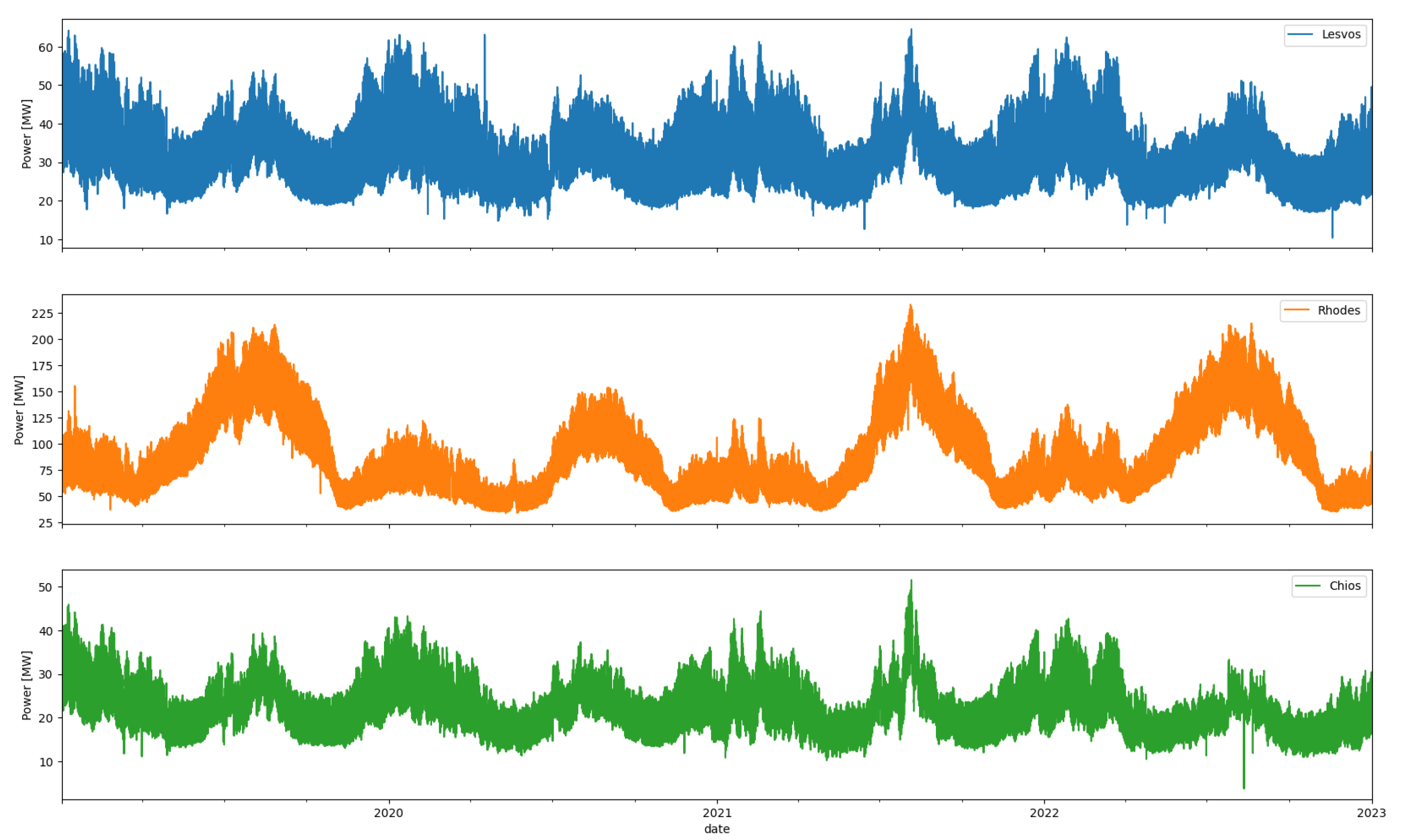
Figure 2.
Monthly average consumption for every island.
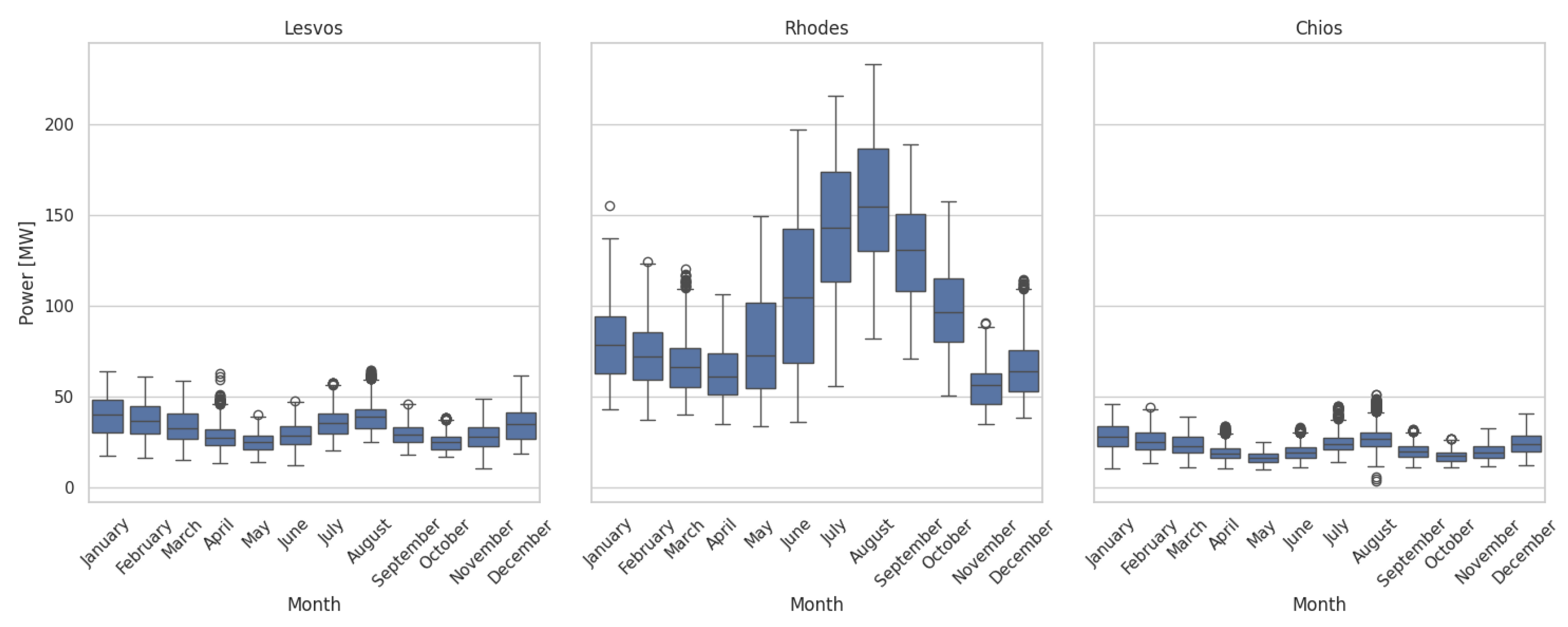
Figure 3.
Hourly average consumption per day for each island.
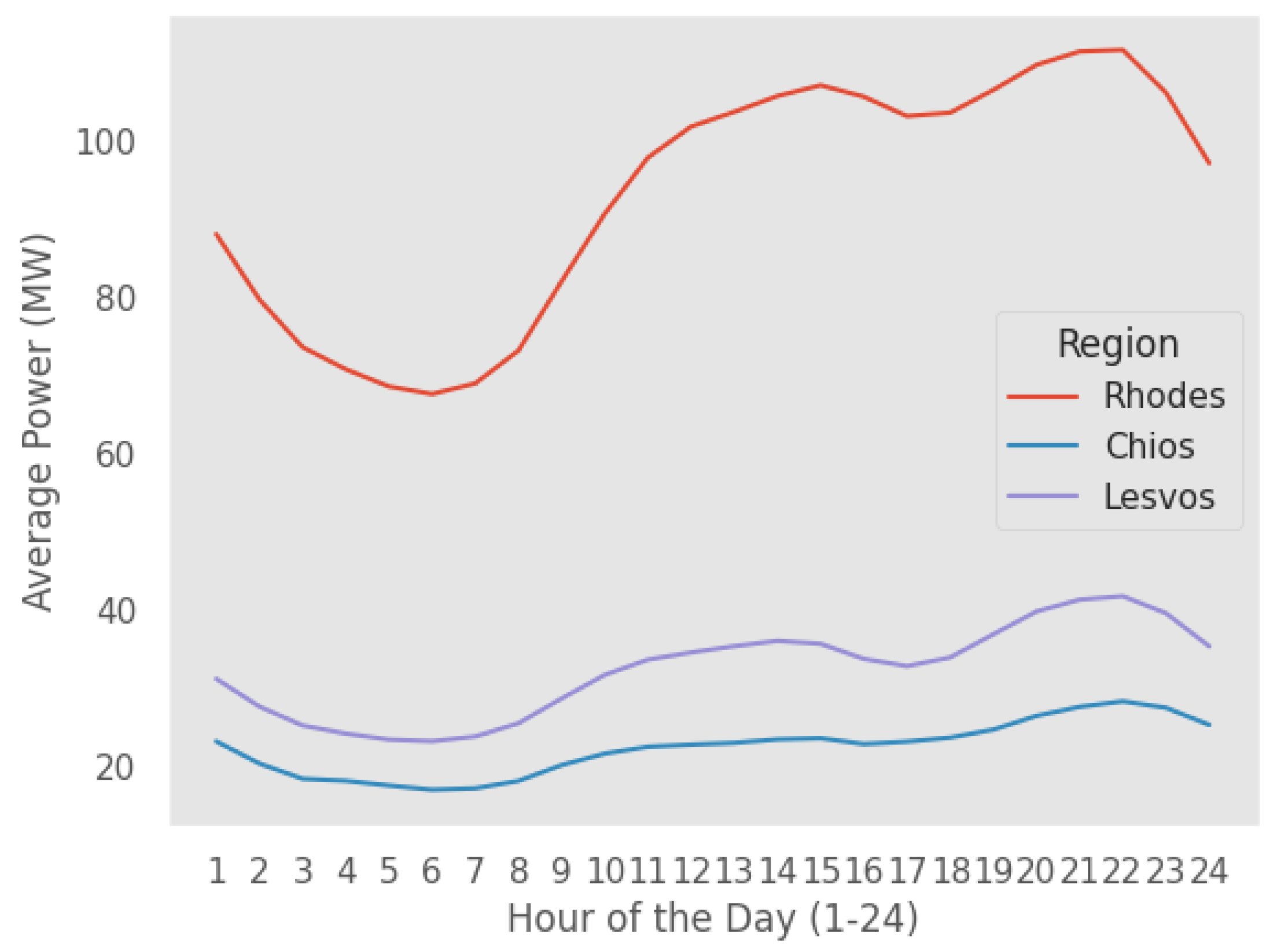
Figure 4.
Day of the week in sine and cosine formulation.
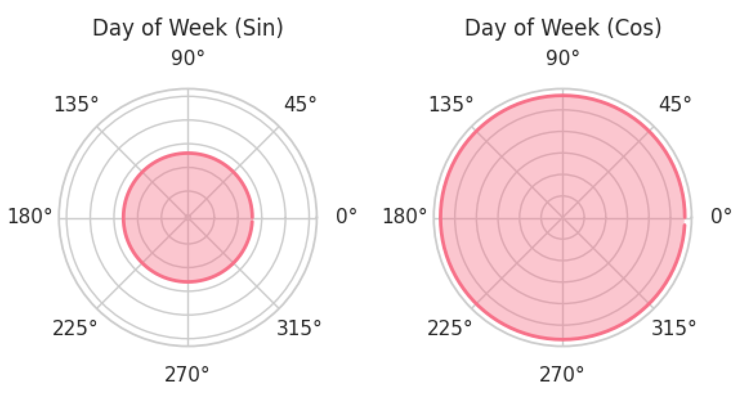
Figure 5.
Sequence-to-sequence forecasting technique.
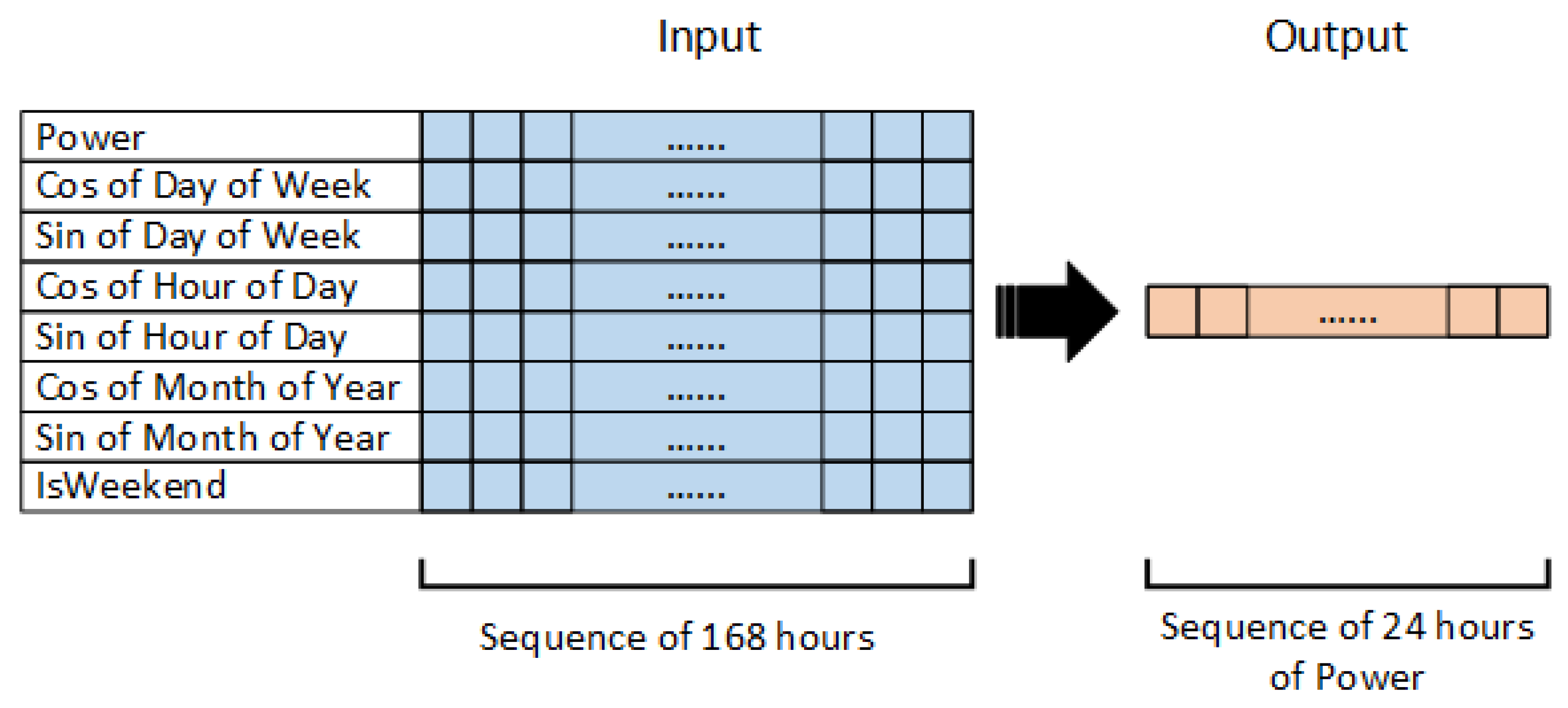
Figure 6.
Correlation Heatmap.
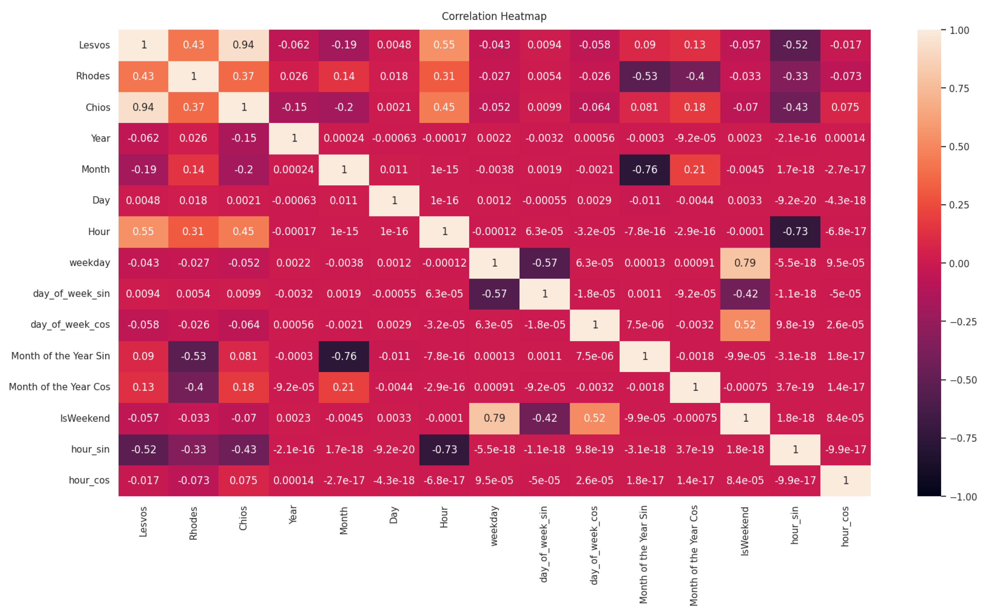
Figure 7.
Multilayer Perceptron Architecture.
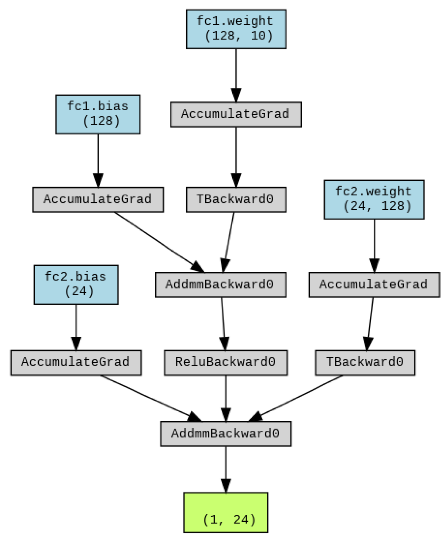
Figure 8.
CNN model architecture.
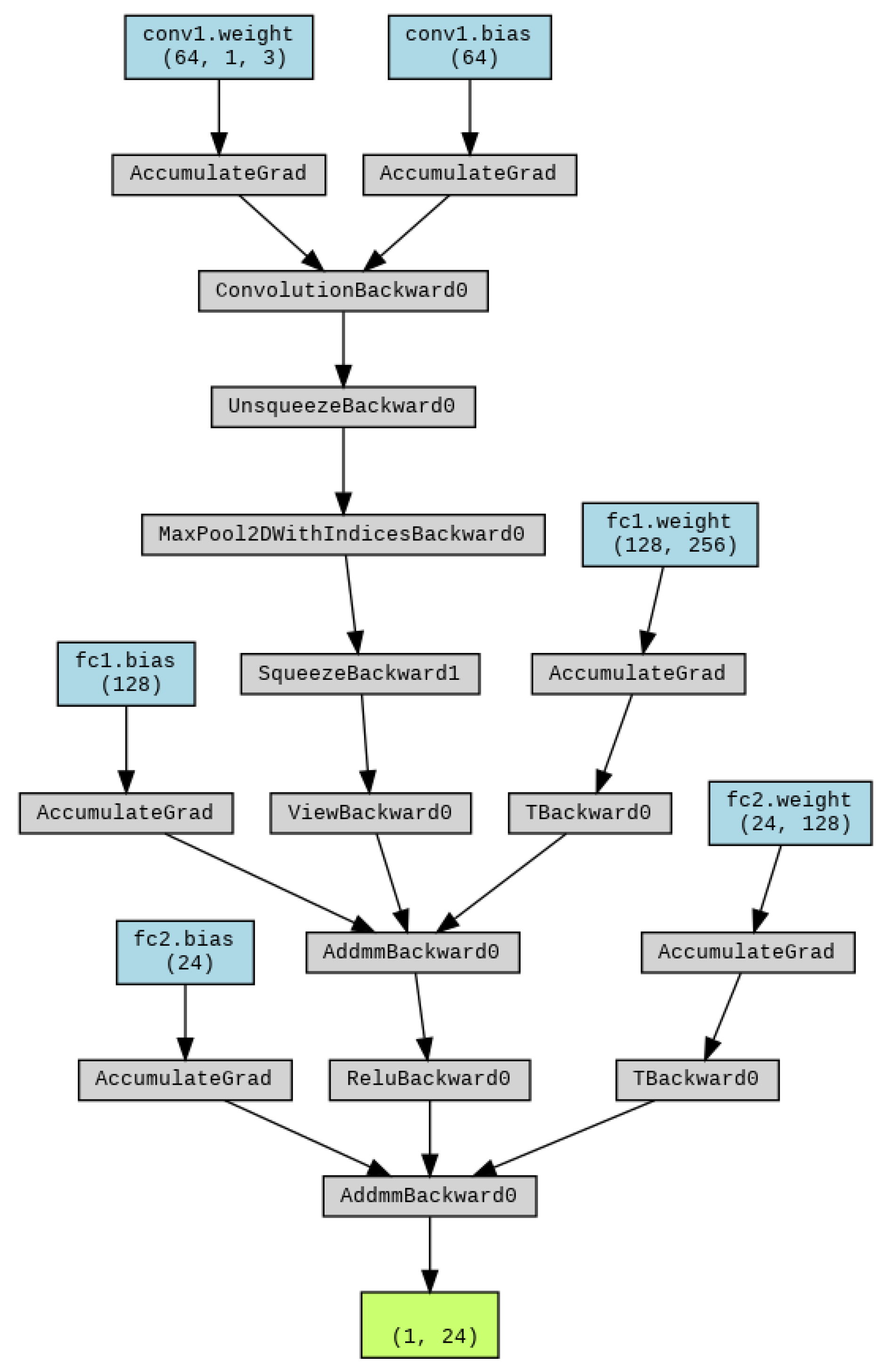
Figure 9.
Ensemble Deep Learning Model Architecture.
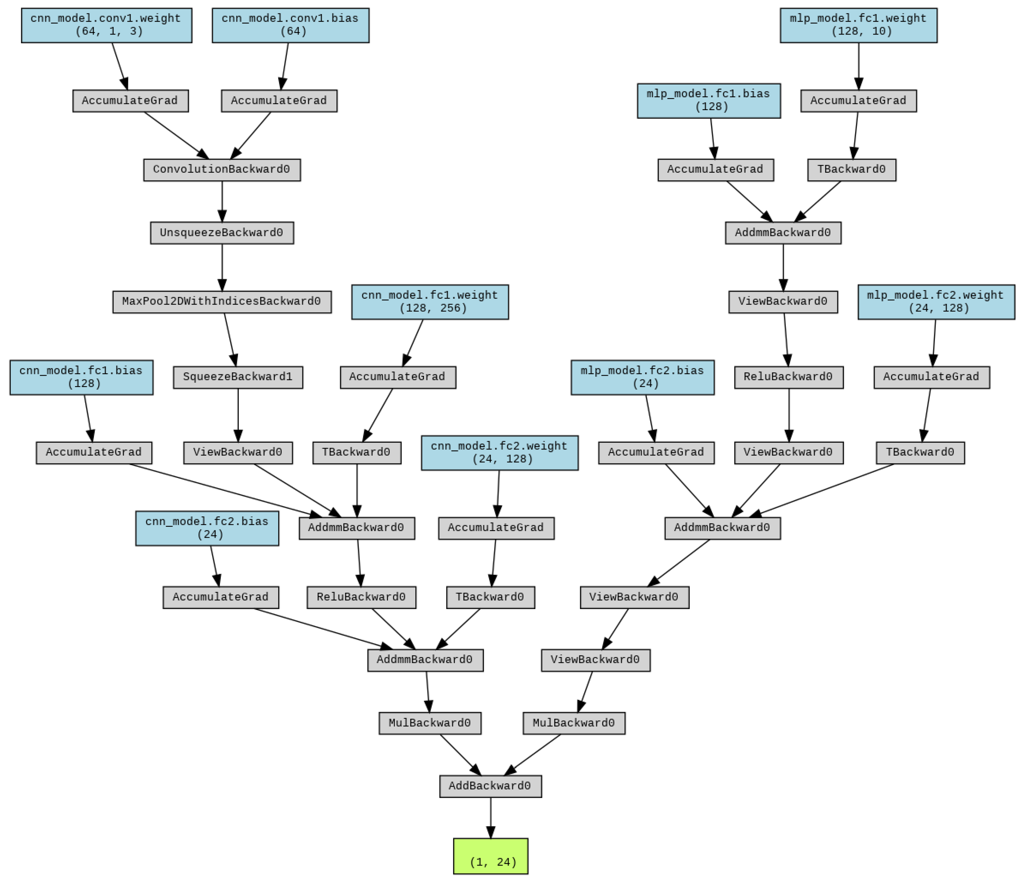
Figure 10.
Deep Transfer Learning Case 1.
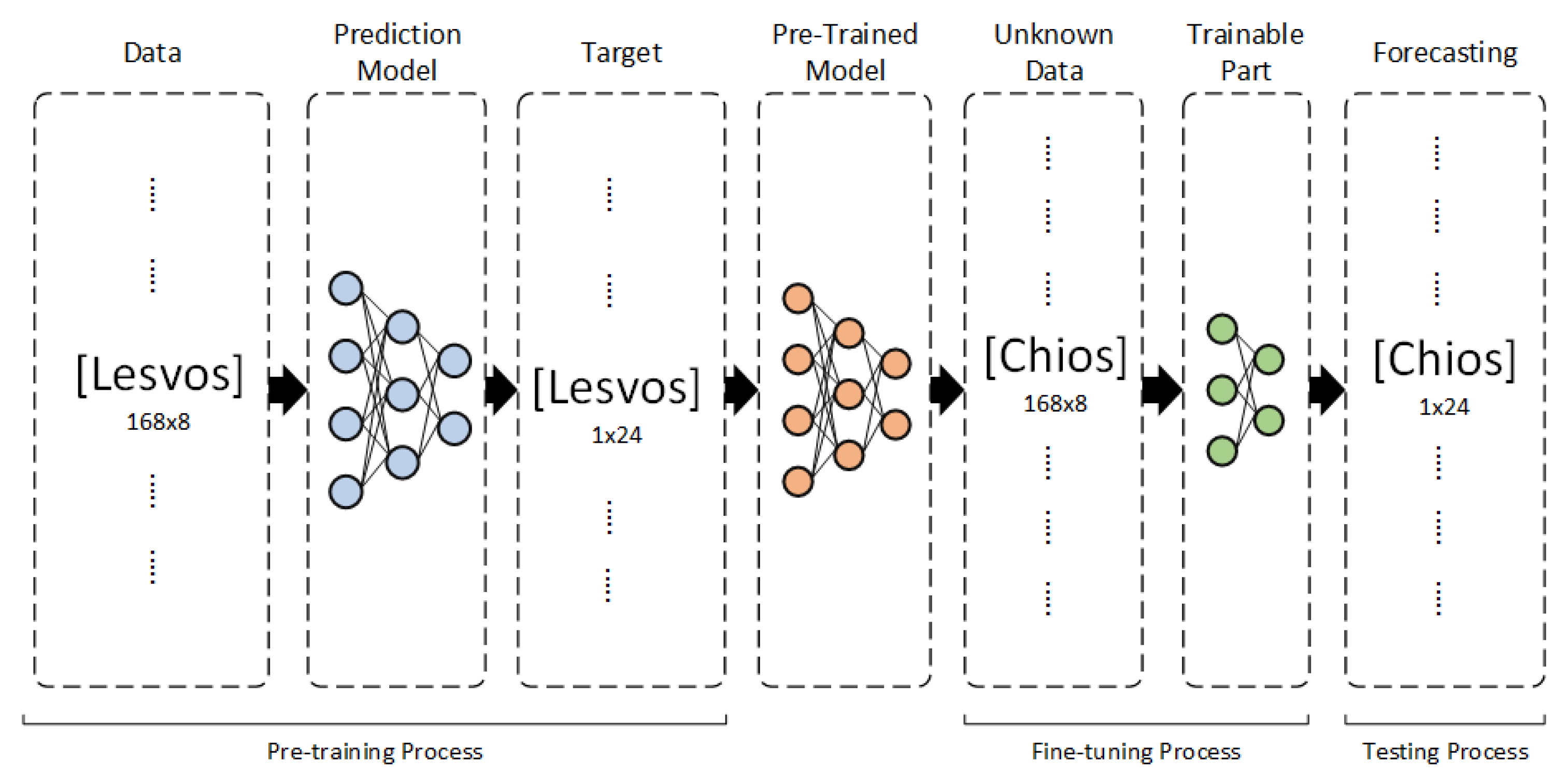
Figure 11.
Deep Transfer Learning Case 2.
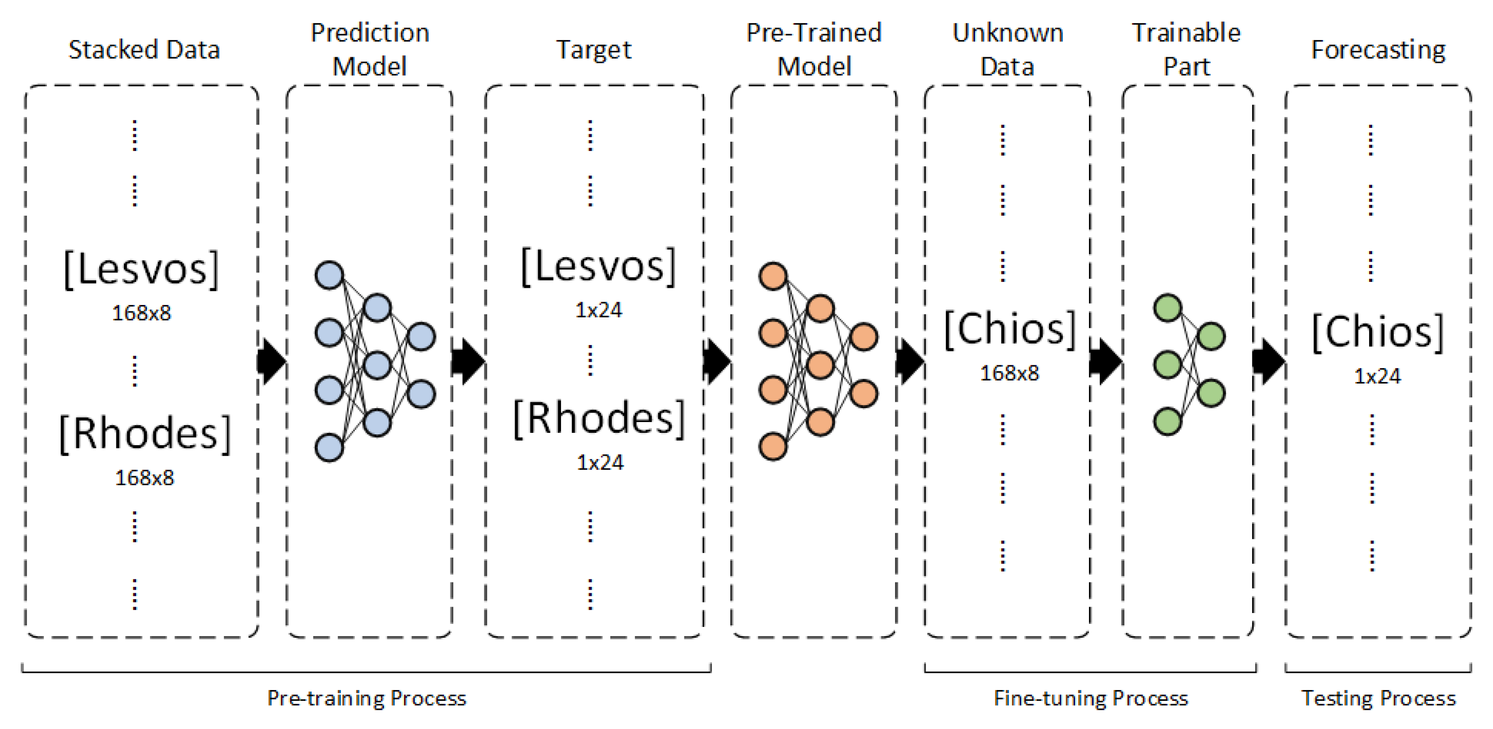
Figure 12.
Deep Transfer Learning Case 3.
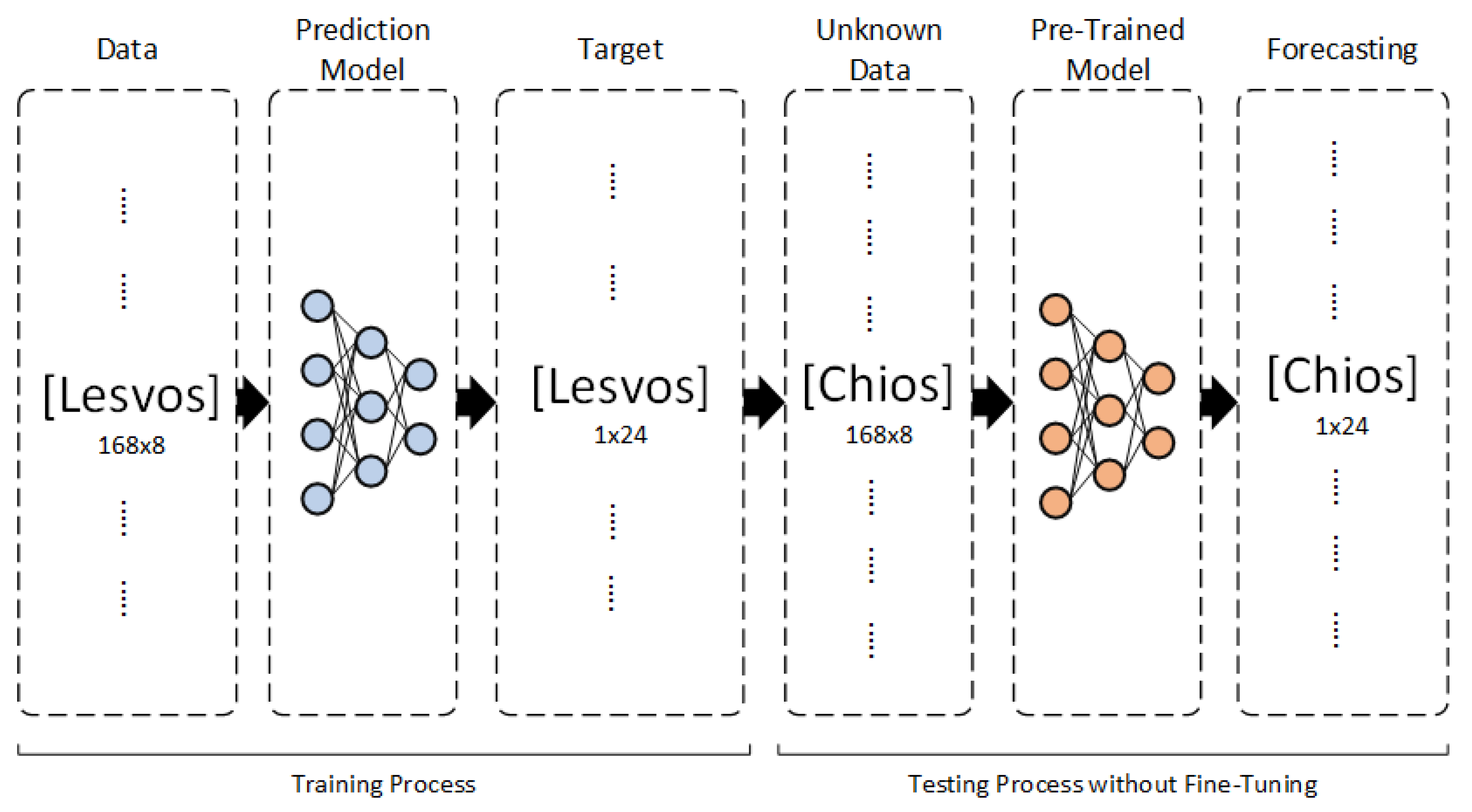
Figure 13.
Multi-task Deep Learning.
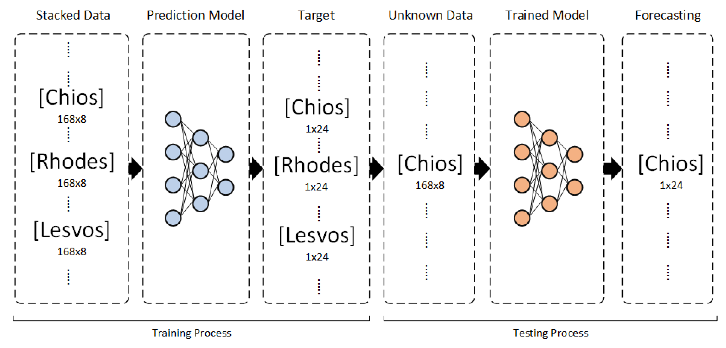
Figure 14.
Variation of MAE for MLP model.
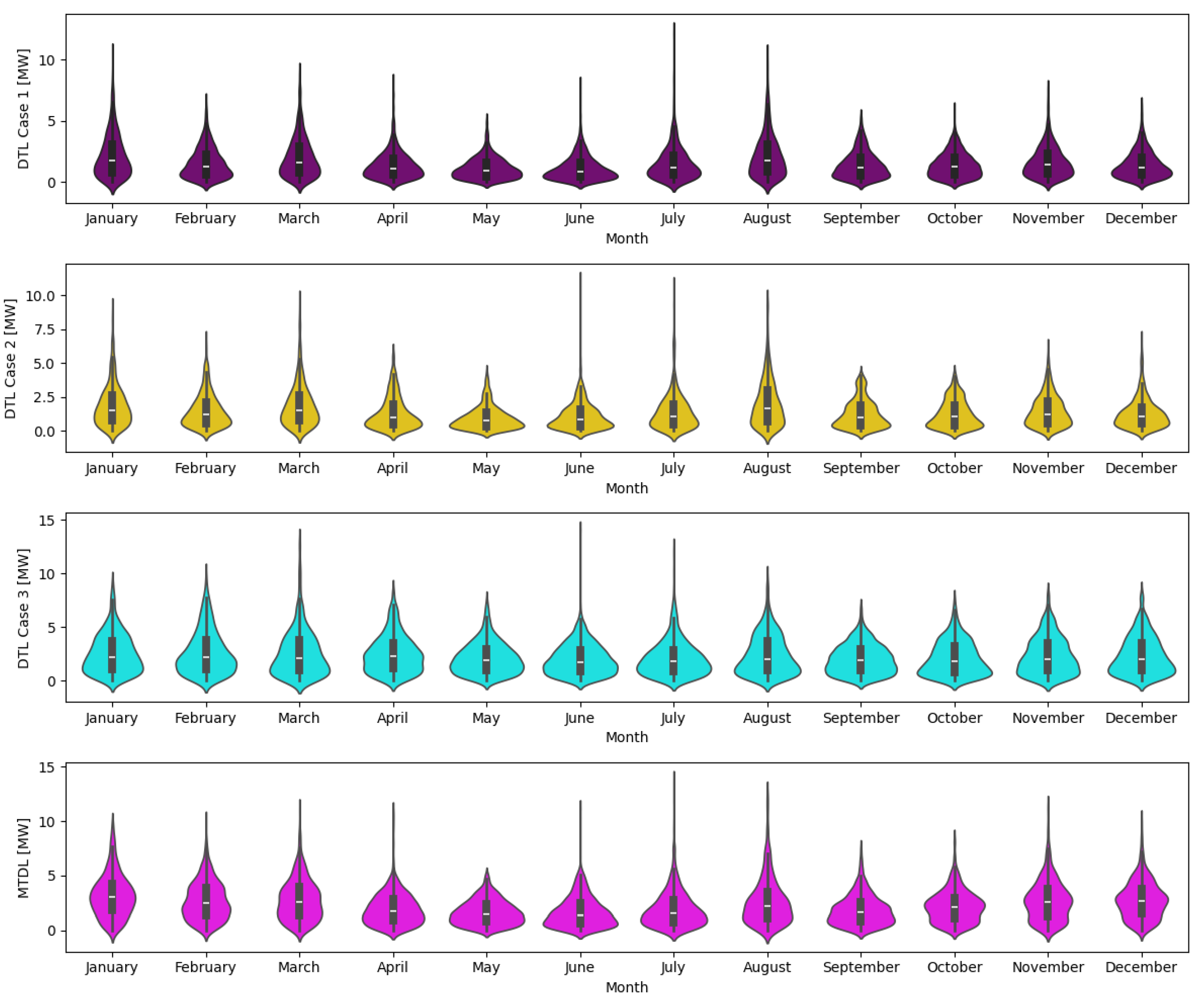
Figure 15.
Variation of MAE for CNN model.
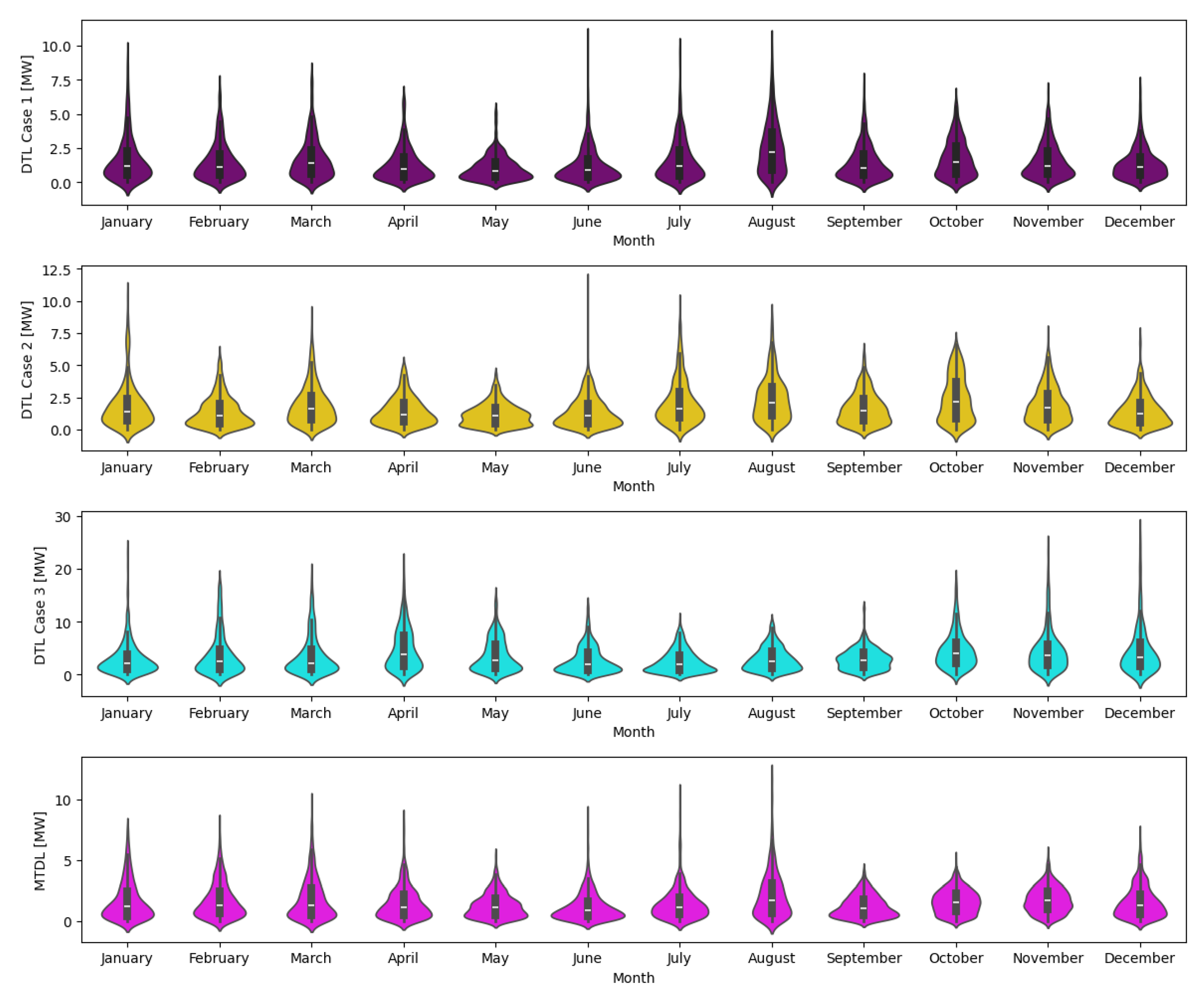
Figure 16.
Variation of MAE for ELM.
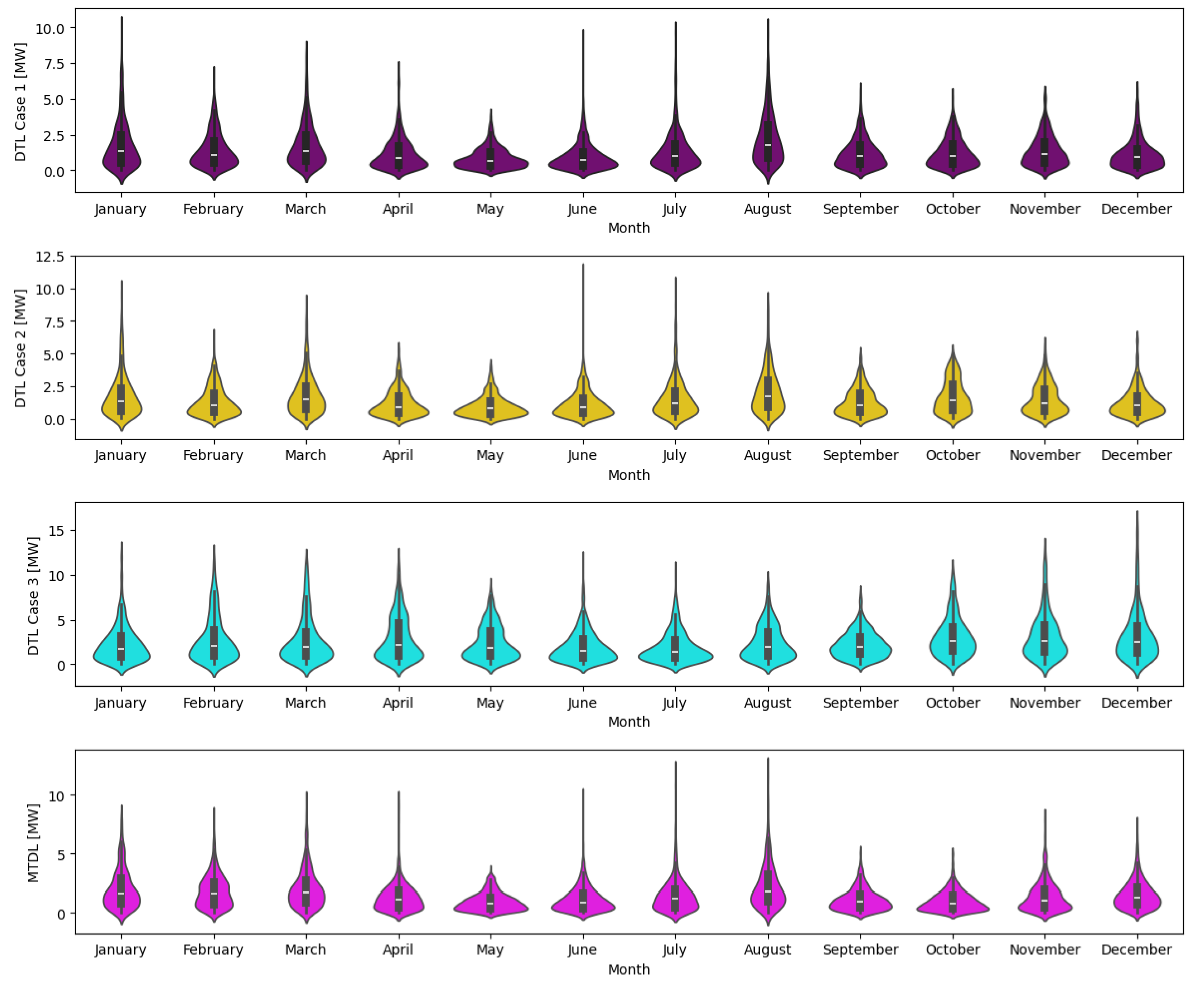
Figure 17.
Comparison of monthly MAE for each forecasting strategy.
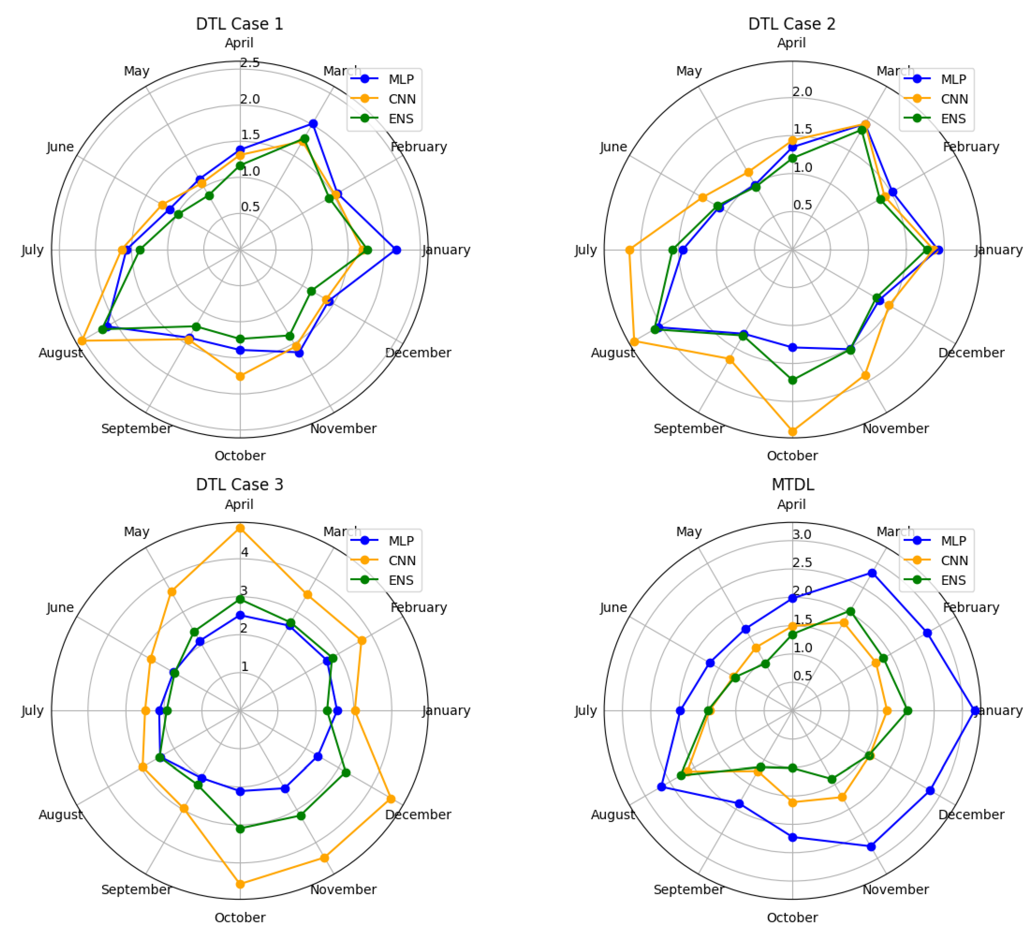
Figure 18.
Comparison of monthly MAPE for each forecasting strategy.
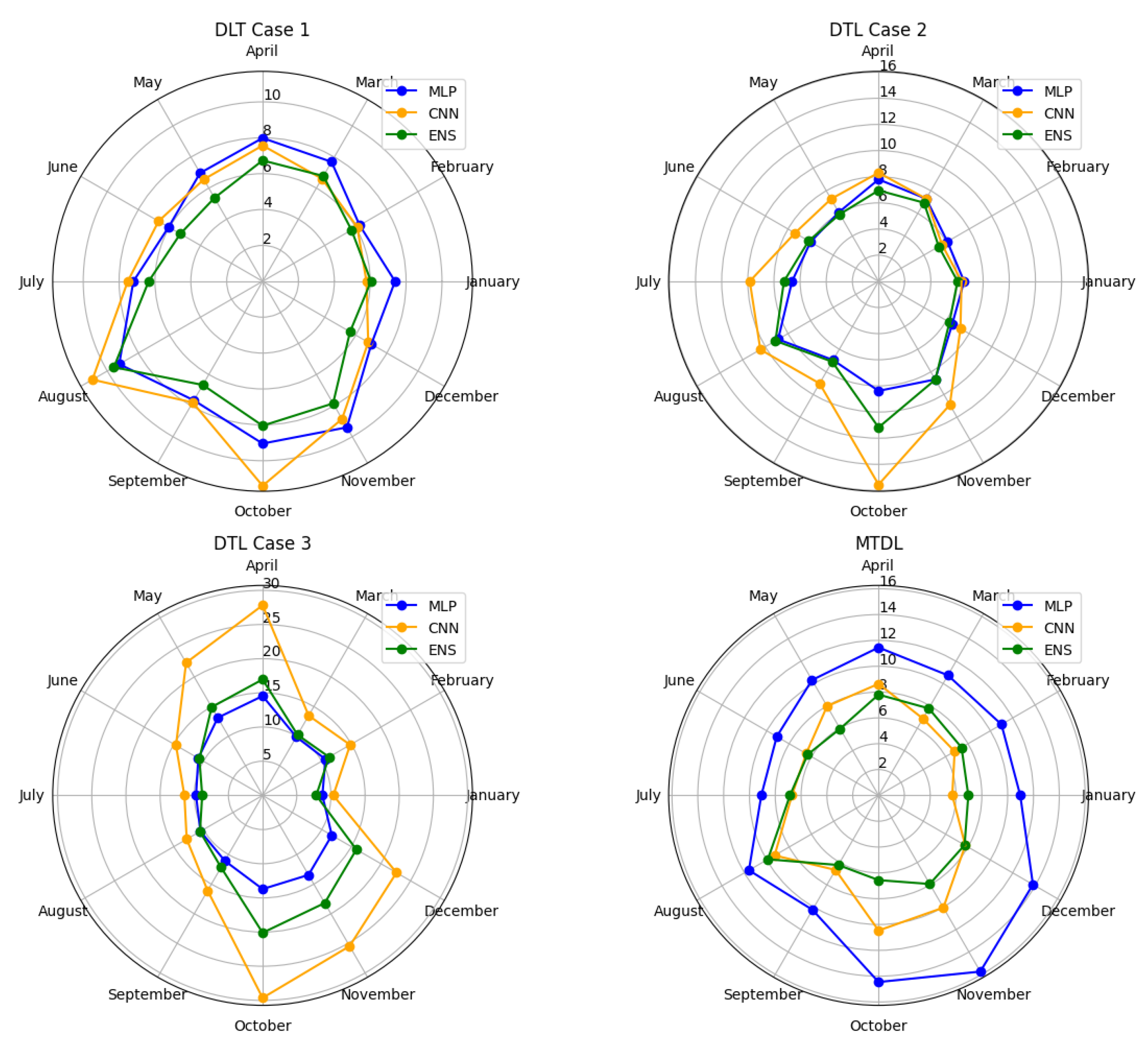
Figure 19.
Comparison of monthly RMSE for each forecasting strategy.
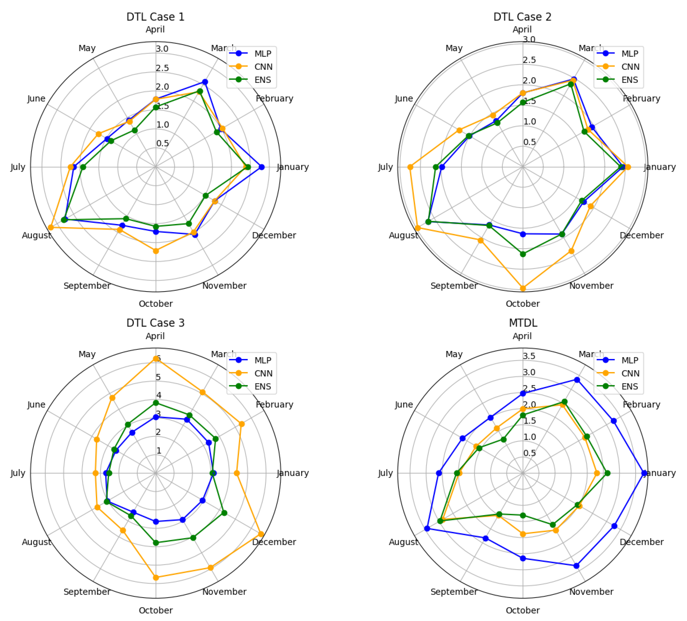

Table 1.
Deep Transfer Learning Case 1.
| Month | |||||||||||||
|---|---|---|---|---|---|---|---|---|---|---|---|---|---|
| Model | Jan | Feb | Mar | Apr | May | June | July | Aug | Sep | Oct | Nov | Dec | |
| MLP | MAE | 2.16 | 1.56 | 2.01 | 1.38 | 1.12 | 1.12 | 1.57 | 2.12 | 1.40 | 1.39 | 1.64 | 1.42 |
| MAPE | 7.38 | 6.24 | 7.68 | 7.98 | 6.97 | 6.05 | 7.01 | 9.23 | 7.66 | 9.04 | 9.39 | 7.00 | |
| RMSE | 2.79 | 1.98 | 2.59 | 1.78 | 1.41 | 1.48 | 2.15 | 2.76 | 1.78 | 1.70 | 2.06 | 1.79 | |
| R2 | 0.83 | 0.87 | 0.82 | 0.67 | 0.73 | 0.74 | 0.63 | 0.08 | 0.75 | 0.53 | 0.70 | 0.82 | |
| CNN | MAE | 1.69 | 1.52 | 1.73 | 1.31 | 1.06 | 1.24 | 1.63 | 2.52 | 1.43 | 1.75 | 1.54 | 1.38 |
| MAPE | 5.57 | 6.07 | 6.60 | 7.57 | 6.55 | 6.69 | 7.46 | 10.95 | 7.79 | 11.39 | 8.85 | 6.79 | |
| RMSE | 2.37 | 2.03 | 2.28 | 1.78 | 1.38 | 1.74 | 2.25 | 3.19 | 1.90 | 2.20 | 1.98 | 1.79 | |
| R2 | 0.88 | 0.87 | 0.86 | 0.68 | 0.74 | 0.64 | 0.59 | 0.11 | 0.70 | 0.21 | 0.73 | 0.82 | |
| ELM | MAE | 1.76 | 1.42 | 1.77 | 1.16 | 0.86 | 0.98 | 1.38 | 2.20 | 1.22 | 1.23 | 1.37 | 1.14 |
| MAPE | 5.87 | 5.72 | 6.77 | 6.73 | 5.36 | 5.29 | 6.24 | 9.57 | 6.67 | 8.04 | 7.82 | 5.62 | |
| RMSE | 2.42 | 1.84 | 2.31 | 1.57 | 1.12 | 1.36 | 1.91 | 2.80 | 1.58 | 1.57 | 1.73 | 1.51 | |
| R2 | 0.88 | 0.89 | 0.86 | 0.75 | 0.83 | 0.78 | 0.71 | 6.25 | 0.80 | 0.61 | 0.80 | 0.87 | |
Table 2.
Deep Transfer Learning Case 2.
| Month | |||||||||||||
|---|---|---|---|---|---|---|---|---|---|---|---|---|---|
| Model | Jan | Feb | Mar | Apr | May | June | July | Aug | Sep | Oct | Nov | Dec | |
| MLP | MAE | 1.91 | 1.51 | 1.91 | 1.34 | 0.98 | 1.11 | 1.44 | 2.04 | 1.28 | 1.28 | 1.51 | 1.32 |
| MAPE | 6.50 | 6.07 | 7.29 | 7.79 | 6.24 | 6.01 | 6.61 | 8.87 | 6.95 | 8.38 | 8.66 | 6.51 | |
| RMSE | 2.44 | 1.94 | 2.47 | 1.80 | 1.29 | 1.50 | 1.98 | 2.67 | 1.64 | 1.63 | 1.89 | 1.71 | |
| R2 | 0.87 | 0.88 | 0.84 | 0.67 | 0.77 | 0.73 | 0.69 | 0.15 | 0.78 | 0.57 | 0.75 | 0.84 | |
| CNN | MAE | 1.85 | 1.40 | 1.91 | 1.43 | 1.17 | 1.37 | 2.14 | 2.40 | 1.66 | 2.39 | 1.90 | 1.46 |
| MAPE | 6.26 | 5.60 | 7.29 | 8.30 | 7.27 | 7.38 | 9.85 | 10.44 | 9.02 | 15.51 | 10.90 | 7.23 | |
| RMSE | 2.56 | 1.83 | 2.43 | 1.80 | 1.46 | 1.79 | 2.76 | 2.96 | 2.06 | 2.96 | 2.36 | 1.90 | |
| R2 | 0.86 | 0.89 | 0.84 | 0.67 | 0.71 | 0.62 | 0.39 | 0.02 | 0.66 | 0.08 | 0.61 | 0.80 | |
| ELM | MAE | 1.76 | 1.32 | 1.82 | 1.20 | 0.95 | 1.14 | 1.57 | 2.10 | 1.30 | 1.71 | 1.51 | 1.27 |
| MAPE | 6.03 | 5.31 | 6.94 | 6.95 | 5.92 | 6.17 | 7.23 | 9.10 | 7.09 | 11.17 | 8.68 | 6.26 | |
| RMSE | 2.38 | 1.72 | 2.33 | 1.57 | 1.23 | 1.52 | 2.12 | 2.66 | 1.65 | 2.12 | 1.89 | 1.65 | |
| R2 | 0.88 | 0.91 | 0.85 | 0.75 | 0.80 | 0.72 | 0.64 | 0.16 | 0.78 | 0.27 | 0.75 | 0.85 | |
Table 3.
Deep Transfer Learning Case 3.
| Month | |||||||||||||
|---|---|---|---|---|---|---|---|---|---|---|---|---|---|
| Model | Jan | Feb | Mar | Apr | May | June | July | Aug | Sep | Oct | Nov | Dec | |
| MLP | MAE | 2.56 | 2.65 | 2.58 | 2.51 | 2.12 | 2.01 | 2.12 | 2.42 | 2.03 | 2.10 | 2.34 | 2.37 |
| MAPE | 8.75 | 10.60 | 9.87 | 14.54 | 13.12 | 10.86 | 9.74 | 10.51 | 11.05 | 13.71 | 13.43 | 11.69 | |
| RMSE | 3.14 | 3.32 | 3.38 | 3.06 | 2.56 | 2.48 | 2.71 | 3.03 | 2.44 | 2.62 | 2.91 | 2.94 | |
| R2 | 0.79 | 0.64 | 0.69 | 0.05 | 0.10 | 0.27 | 0.41 | -0.10 | 0.52 | -0.11 | 0.41 | 0.51 | |
| CNN | MAE | 3.02 | 3.69 | 3.53 | 4.81 | 3.62 | 2.71 | 2.49 | 2.95 | 2.96 | 4.55 | 4.45 | 4.59 |
| MAPE | 10.34 | 14.79 | 13.48 | 27.82 | 22.40 | 14.63 | 11.45 | 12.82 | 16.09 | 29.63 | 25.47 | 22.62 | |
| RMSE | 4.39 | 5.37 | 5.10 | 6.25 | 4.75 | 3.70 | 3.27 | 3.67 | 3.58 | 5.66 | 5.93 | 6.59 | |
| R2 | 0.58 | 0.05 | 0.29 | -2.96 | -2.08 | -0.64 | 0.14 | -0.61 | -0.05 | -4.18 | -1.45 | -1.45 | |
| ELM | MAE | 2.29 | 2.80 | 2.68 | 2.93 | 2.41 | 1.98 | 1.92 | 2.44 | 2.23 | 3.09 | 3.18 | 3.21 |
| MAPE | 7.85 | 11.22 | 10.22 | 16.96 | 14.91 | 10.68 | 8.84 | 10.58 | 12.16 | 20.10 | 18.18 | 15.84 | |
| RMSE | 3.07 | 3.76 | 3.65 | 3.82 | 3.06 | 2.61 | 2.55 | 3.09 | 2.67 | 3.78 | 4.05 | 4.27 | |
| R2 | 0.80 | 0.54 | 0.64 | -0.48 | -0.28 | 0.19 | 0.48 | -0.14 | 0.42 | -1.30 | -0.14 | -0.03 | |
Table 4.
Multi-task Deep Learning.
| Month | |||||||||||||
|---|---|---|---|---|---|---|---|---|---|---|---|---|---|
| Model | Jan | Feb | Mar | Apr | May | June | July | Aug | Sep | Oct | Nov | Dec | |
| MLP | MAE | 3.21 | 2.74 | 2.81 | 1.98 | 1.66 | 1.69 | 1.98 | 2.67 | 1.88 | 2.22 | 2.75 | 2.80 |
| MAPE | 10.97 | 10.99 | 10.73 | 11.45 | 10.31 | 9.10 | 9.06 | 11.50 | 10.23 | 14.45 | 15.75 | 13.80 | |
| RMSE | 3.75 | 3.24 | 3.36 | 2.47 | 2.00 | 2.16 | 2.61 | 3.43 | 2.32 | 2.64 | 3.31 | 3.27 | |
| R2 | 0.70 | 0.66 | 0.69 | 0.38 | 0.46 | 0.44 | 0.45 | -0.40 | 0.56 | -0.12 | 0.24 | 0.40 | |
| CNN | MAE | 1.67 | 1.69 | 0.80 | 1.49 | 1.28 | 1.20 | 1.46 | 2.14 | 1.22 | 1.60 | 1.75 | 1.57 |
| MAPE | 5.62 | 6.78 | 6.86 | 8.63 | 7.97 | 6.47 | 6.58 | 9.30 | 6.66 | 10.46 | 10.03 | 7.75 | |
| RMSE | 2.30 | 2.22 | 2.45 | 1.99 | 1.62 | 1.67 | 1.98 | 2.87 | 1.51 | 1.88 | 2.04 | 2.02 | |
| R2 | 0.89 | 0.84 | 0.84 | 0.60 | 0.64 | 0.67 | 0.69 | 0.01 | 0.82 | 0.43 | 0.70 | 0.77 | |
| ELM | MAE | 2.03 | 1.85 | 2.03 | 1.35 | 0.96 | 1.17 | 1.49 | 2.28 | 1.14 | 1.00 | 1.38 | 1.56 |
| MAPE | 6.86 | 7.42 | 7.77 | 7.80 | 5.96 | 6.33 | 6.86 | 9.89 | 6.22 | 6.56 | 7.92 | 7.69 | |
| RMSE | 2.61 | 2.28 | 2.56 | 1.80 | 1.21 | 1.57 | 2.05 | 2.96 | 1.46 | 1.30 | 1.84 | 1.95 | |
| R2 | 0.85 | 0.83 | 0.82 | 0.67 | 0.80 | 0.71 | 0.66 | -0.05 | 0.83 | 0.73 | 0.77 | 0.79 | |
Disclaimer/Publisher’s Note: The statements, opinions and data contained in all publications are solely those of the individual author(s) and contributor(s) and not of MDPI and/or the editor(s). MDPI and/or the editor(s) disclaim responsibility for any injury to people or property resulting from any ideas, methods, instructions or products referred to in the content. |
© 2024 by the authors. Licensee MDPI, Basel, Switzerland. This article is an open access article distributed under the terms and conditions of the Creative Commons Attribution (CC BY) license (http://creativecommons.org/licenses/by/4.0/).
Copyright: This open access article is published under a Creative Commons CC BY 4.0 license, which permit the free download, distribution, and reuse, provided that the author and preprint are cited in any reuse.


