Submitted:
09 April 2024
Posted:
10 April 2024
You are already at the latest version
Abstract
This paper presents a compartmental model aimed at investigating the pharmacokinetics of medical THC after oral administration. The model was developed to be multi-compartmental, describing the kinetics of THC and its metabolites in bodily tissues. Utilizing the law of mass action, the model was converted into ordinary differential equations (ODEs), illustrating the rate of concentration changes of THC and its metabolites in each compartment. Subsequently, we applied the nonstandard finite difference (NSFD) method to construct numerical solution schemes. These schemes were implemented in the MATLAB program, along with estimated pharmacokinetic rate constants. The results of the investigation demonstrate that the simulation curves depicting the plasma concentration-time profiles of THC and THC-OH closely resemble the actual data samples, indicating that this model accurately describes the pharmacokinetics of medical THC and its metabolites. Moreover, the model exhibits predictive capabilities regarding the pharmacokinetics of THC and its metabolites in various tissues. Consequently, the model serves as a valuable tool for enhancing our understanding of the pharmacokinetics of THC and its metabolites and for guiding adjustments to dosage and administration durations for oral medical THC products.
Keywords:
compartment model
; delta9-tetrahydrocannabinol (THC)
; nonstandard finite difference (NSFD)
; oral administration
; pharmacokinetics
1. Introduction
Delta9-tetrahydrocannabinol (THC), one of the cannabinoids found in the cannabis plant, possesses several clinically useful pharmacological characteristics [1]. As a result, THC is extracted and developed into a medical product, serving as an alternative medicine to treat patients who do not respond to modern medicine. This includes patients experiencing nausea and vomiting from chemotherapy, medication-resistant epilepsy, anorexia in AIDS patients, and those seeking to improve the quality of life in palliative care. Several studies show that medical THC has positive effects in treating various diseases [2,3]. On the other hand, THC is a psychoactive chemical that can be addictive if taken in inappropriate amounts. Therefore, the administration of medical THC to patients must be approached with caution because the precise and appropriate dosage for various patient groups in the administration of different medical THC products has not yet been established. The general advice is to start with a small dosage, for example, administering it once a day, and gradually increase the dosage when the patient does not experience side effects. Therefore, having a tool to help describe the pharmacokinetics of medical THC will increase our understanding of medical THC pharmacokinetics and can also be used to guide the determination of the dosage and administration duration of medical THC products.
Currently, various forms of medical THC products are available, catering to different treatment needs that demand rapid bloodstream absorption, ranging from oral, inhalation, and smoking to injection. Among these, oral dosage forms like capsules or tablets are widely preferred due to their convenience and straightforward dosage determination. While previous research has delved into THC pharmacokinetics post-smoking [4], this study will focus on investigating the pharmacokinetics of clinical THC administered orally. After oral administration, THC is absorbed through the gastrointestinal tract (stomach and small intestine) with a bioavailability of about 0.1-0.2% [5]. Subsequently, it enters the liver via the hepatic portal vein for first-pass metabolism. In the liver, THC is metabolized by the enzymes CYP2C and CYP3A into its main metabolites, THC-OH and THCCOOH. THC-OH is the primary psychoactive metabolite, while THCCOOH is a secondary metabolite and is not psychoactive [6]. The remaining THC and both of its metabolites pass through the heart before entering the bloodstream. Both THC and THC-OH simultaneously enter the brain. Approximately 20% of THC and other cannabinoids are excreted in urine, with more than 65% eliminated in feces within 5 days [7].
Compartment modeling is another method that can be employed to study pharmacokinetics, encompassing processes such as absorption, distribution, metabolism, and excretion. It is a mathematical technique used to represent the entire body by dividing it into compartments. This modeling approach helps avoid challenges and reduces costs associated with clinical studies. Previous research studies have proposed compartment models to describe the complex pharmacokinetics of THC. For instance, in 2015, Jules and their group [8] provided a four-compartment pharmacokinetic model for THC after oral, intravenous, and pulmonary dosing. In 2017, Rakesh [9] conducted a study on the pharmacokinetics and pharmacodynamics of THC and its active metabolite using effect compartment modeling-based approaches. In 2020, Cristina and their team [10] constructed a population multi-compartment pharmacokinetic model for THC and its active and inactive metabolites after controlled smoked cannabis delivery. Additionally, in 2023, we created a compartment model to study the pharmacokinetics of THC and its metabolites after smoking [4]. Usually, we can solve analytical solutions when building a compartment model with one or two compartments. However, because the system of differential equations for a three- or multi-compartment model is large, it becomes difficult to derive an analytical solution. Therefore, numerical methods were introduced to help reduce the challenge of solving analytical solutions for the multi-compartment model. One of the numerical methods used to solve the ODE system of the compartment pharmacokinetic model is the nonstandard finite difference method (NSFD). This method evolved from the standard finite difference method (SFD) developed by Mickens [11,12] to construct numerical solution schemes. Previous studies have shown that the NSFD method provides more stable numerical results compared to the SFD method, regardless of the chosen step size [13,14,15,16].
In this study, we developed a compartmental model based on our previous research, which focused on the compartmental pharmacokinetic model of medical THC following smoking [4]. The objective of this work was to develop a compartmental model to comprehensively investigate the pharmacokinetics of medical THC and its metabolites in the body after oral administration. The model was converted into ordinary differential equations (ODEs) to depict the rate of concentration change of THC and its metabolites in bodily compartments, utilizing the law of mass action. For the simulation, we will find numerical solutions by applying the NSFD method to create numerical solution schemes. These schemes were then implemented in the MATLAB program, along with the estimated pharmacokinetic rate constants of THC and its metabolites, to generate simulation curves.
2. Methodology
In this section, we develop a multi-compartment model to describe the pharmacokinetics of THC after oral administration. The compartment model is converted into ordinary differential equations (ODEs) to describe the rate of change of THC and its metabolite concentrations in each compartment, using the law of mass action. Afterward, we apply the nonstandard finite difference method (NSFD) to transform the ODEs into numerical solution schemes. Additionally, we provide the estimated pharmacokinetic rate constants used to simulate the results, including examples of actual plasma concentrations of THC and THC-OH that are compared with our simulation results.
2.1. Compartmental Modeling
Here, we considered dividing the compartment model representing the body into four phases: the first phase encompassed the absorption compartment, representing the gastrointestinal tract, to elucidate THC absorption. The second phase dealt with the pharmacokinetics of THC, while the third phase focused on the pharmacokinetics of THC-OH. The fourth phase examined the pharmacokinetics of THCCOOH in plasma. In this model, we considered the pharmacokinetics of THC and THC-OH in the blood and tissues by dividing the body into three physiologically significant compartments: the central compartment, representing the blood (plasma) or systemic circulation; the rapidly equilibrating tissue compartment, representing organs like the liver, lungs, and kidneys; and the slowly equilibrating tissue compartment, representing tissues such as muscle, fat, and bone. Additionally, we created effect compartments for THC and THC-OH to describe their concentrations at the sites of effect.
We defined rate constants for the absorption, distribution, metabolism, and excretion of THC and its metabolites in each compartment. The concentrations were represented as follows: for THC in the absorption compartment (gastrointestinal tract), for THC in the central compartment (plasma), for THC in the rapidly equilibrating tissue compartment, for THC in the slowly equilibrating tissue compartment, and for THC in the effect compartment. for THC-OH in the central compartment, for THC-OH in the rapidly equilibrating tissue compartment, for THC-OH in the slowly equilibrating tissue compartment, for THC-OH in the effect compartment, and for THCCOOH in the central compartment. We let be the absorption rate constant of THC. The distribution rate constants of THC in each compartment were denoted as , , , , and . The metabolic rate constants of THC to THC-OH and THCCOOH were represented by and , respectively. For THC-OH, the distribution rate constants in each compartment were , , , , and , while was the metabolic rate constant of THC-OH to THCCOH. The elimination rate constants of THC-OH and THCCOOH from the central compartment were and , respectively. Additionally, and denoted the elimination rate constants of THC and THC-OH from the effect compartment. This representation was illustrated in Figure 1.
By applying the law of mass action to the compartment model illustrated in Figure 1, we derived a set of ordinary differential equations representing the rate of change of THC and its metabolite concentrations in each compartment, as follows:
where
Next, we will apply the NSFD method to System 1 to construct numerical solution schemes, thereby reducing the challenge of solving analytical solutions for large systems of equations.
2.2. NSFD Schemes
The nonstandard finite difference method (NSFD), a numerical approach, has been used in continuous models. It was developed from the standard finite difference method (SFD) by Mickens [11,12]. It serves as an alternative method to ensure the stability of numerical solutions, irrespective of the chosen step size. The NSFD procedures are based on the following rules:
1) The following represents the discrete first derivative:
where and depends on step-size and satisfy the conditions:
and can have different functions from one another. While specific forms for a given equation can be readily found, there are currently no general guidelines for choosing the functions and . Frequently employed functional representations for and are
where is some parameter appearing in the differential equations.
2) Both linear and nonlinear terms may require a nonlocal representation on the discrete computational; for example:
Preliminary rules exist for constructing denominator functions for a system of coupled first-order ordinary differential equations:
1) Form an initial, finite difference model by replacing all first-derivatives by discrete forward-Euler terms.
2) For a particular discrete equation, in general, its dependent variable will occur linearly in its evaluation at the -th time step. Solve for this dependent variable at the -th time step in terms of all other dependent variables evaluated at the k-th time step.
3) The denominator function can be chosen as follows
If a factor in a given discrete equation has an expression of the form , where is made up of one or more parameters that occur in the original differential equations.
4) In the discrete finite-difference schemes constructed in (1), replace h by the appropriate .
5) For the case where , use the denominator function .
Therefore, from the ordinary differential equations in Equation (1), by applying the NSFD method to convert them into numerical solution schemes, we obtain
By rearranging System (2), we obtain the solution schemes as follows:
where the various depend on step-size (h) and are written in the functional form as follows:
2.3. Pharmacokinetic Parameters
To simulate the results, we needed to know the pharmacokinetic rate constants of THC and its metabolites. In this study, we derived these rate constants from our previous investigation on the pharmacokinetics of THC and its metabolites after smoking [4], adjusting them to obtain simulation results as close to the actual data as possible. Therefore, we obtained the estimated pharmacokinetic rate constants for THC and THC-OH, as shown in Table 1.
2.4. Actual Data
The actual data sample we used for comparison with the simulation results in this study consisted of the plasma concentrations of THC and THC-OH after the oral administration of 10 mg of THC, based on a study conducted by Guy and Robson [17]. Experimental data from the clinical study are shown in Table 2.
From the actual data sample as shown in Table (Table 2), we will compare it with the simulated results of the concentration of THC and THC-OH to investigate any errors, which we will discuss in the conclusion and discussion section.
3. Simulation Results
For the simulations, we utilized the NSFD scheme specified in System (3) and implemented it in the MATLAB program. We employed the estimated pharmacokinetic rate constants from Table 2 and selected a step size (h) of 0.05. Consequently, we obtained simulated concentrations of THC and THC-OH in plasma and other tissues following the oral administration of 10 mg of THC, replicating the experimental conditions of the clinical studies conducted by Guy and Robson [17]. These results are presented in Figure 2 and Figure 3 for THC and THC-OH, respectively. Additionally, the simulated concentrations of THC and THC-OH are illustrated in Figure 4 and Figure 5, respectively.
4. Conclusion and Discussion
In this study, we developed a compartment model to describe the pharmacokinetics of delta9-tetrahydrocannabinol (THC) and its metabolites following oral administration. The compartmental model was converted into ordinary differential equations (ODEs), which represent the rate of change in the concentration of THC and its metabolites in each compartment, using the law of mass action. Subsequently, we applied the nonstandard finite difference method (NSFD) to create numerical solution schemes. These schemes were then implemented in a MATLAB program, along with the estimated pharmacokinetic rate constants, to generate the simulation results. The rate constants used in the simulation were adjusted from our previous study on the pharmacokinetics of THC and its metabolites following smoking.
In the simulation results of THC and THC-OH following the oral administration of 10 mg THC under the conditions of the clinical study by Guy and Robson [17], using the NSFD scheme as depicted in System (3) with a chosen h of 0.05, we observed the following trends:
For THC, the concentration in plasma, denoted as , rapidly increased, reaching a maximum concentration of 4.52 ng/ml between 50 and 55 minutes. Subsequently, it decreased rapidly within the 55-360 minute interval before gradually declining over time. When comparing the simulation results to the actual data from the study by Guy and Robson, we found that the simulated plasma THC concentration curves closely resembled the actual data, with an R-squared value of 0.8167 and an RMSE value of 0.6626. In the absorption compartment, denoted as , the THC concentration rapidly decreased from the initial concentration of 24.85 ng/ml within the 0-200 minute interval and continued to decrease gradually until reaching 0 ng/ml after 200 minutes. The THC concentration in other tissues gradually increased, depending on the distribution rate constants. The maximum concentrations of THC in the rapidly equilibrating tissue, the slowly equilibrating tissue, and the effect site were 3.36 ng/ml at 50-55 minutes, 1.68 ng/ml at 50-55 minutes, and 0.043 ng/ml at 160-235 minutes, respectively. After reaching their maximum concentrations, it gradually decreased to 0 ng/ml over time, as illustrated in Figure 2. The simulated concentration of THC after oral administration of 10 mg in each tissue is depicted in Figure 4.
For THC-OH, we observed a rapid increase in the THC-OH concentration in plasma (), reaching a maximum concentration of 6.76 ng/ml at 105 minutes. When comparing the simulation results to the actual data from the study by Guy and Robson, we found that the simulated plasma THC-OH concentration curve closely resembled the actual data, albeit with a maximum time discrepancy. The R-squared value was 1.0189, and the RMSE value was 0.7848. This discrepancy may be related to the estimated pharmacokinetic parameters. Additionally, we noted an increase in the THC-OH concentration in other tissues to their respective maximum points, followed by a gradual decrease over time. The maximum concentrations of THC-OH in the rapidly equilibrating tissue, the slowly equilibrating tissue, and the effect site were 0.042 ng/ml at 105 minutes, 0.022 ng/ml at 105 minutes, and 1.60 ng/ml at 250-260 minutes, respectively, as depicted in Figure 3. The simulated concentration of THC-OH after oral administration of 10 mg THC in each tissue is shown in Figure 5.
Furthermore, when comparing the simulation results with another study that administered the same initial dosage of 10 mg oral medical THC, such as the previously published study by Nadulski and their team [18], we noted differences in the mean maximum concentrations of THC and THC-OH in plasma ( and , respectively). In their study, the mean maximum concentration of THC was 3.20 ng/ml at a mean maximum time of 63 minutes, while the mean maximum concentration of THC-OH was 4.48 ng/ml at a mean maximum time of 90 minutes. These slight discrepancies between our simulation results and Nadulski’s study may be attributed to variations in the clinical study conditions. Based on our simulation results and the findings from Nadulski’s study, we can infer that following the oral administration of 10 mg of THC, the maximum concentration of THC will range from approximately 3.2 to 4.52 ng/ml, occurring approximately between 50 and 63 minutes. Similarly, the maximum concentration of THC-OH will range from approximately 4.88 to 6.76 ng/ml, occurring approximately between 90 and 105 minutes. Therefore, in subsequent medical THC administrations, it is advisable to wait for the concentrations of THC and THC-OH in plasma to decrease, thereby ensuring that they do not reach excessively high levels.
Based on the simulation results, our model can produce pharmacokinetic curves of THC and its metabolites in plasma after oral administration that are close to the actual data from the study conducted by Guy and Robson. Furthermore, our model can predict the concentration of THC and its metabolites in other bodily compartments, providing an advantage over most clinical studies that only consider or investigate plasma concentrations of THC and its metabolites. Consequently, our model can serve as a tool to advance our understanding of the pharmacokinetics of medical THC, including assisting in determining the dosage and administration duration for oral medical THC products. Moreover, the model shows potential for further refinement and development in the future.
Author Contributions
Conceptualization, T.M. and T.S.; methodology, T.M. and T.S.; software, T.M. ; validation, T.M. and T.S.; formal analysis, T.M. and T.S.; investigation, T.M. and T.S.; resources, T.M.; data curation, T.M. and T.S.; writing—original draft preparation, T.M.; writing—review and editing, T.M. and T.S.; supervision; T.S. All authors have read and agreed to the published version of the manuscript.
Funding
This research received no external funding.
Institutional Review Board Statement
Not applicable.
Informed Consent Statement
Not applicable.
Data Availability Statement
Not applicable.
Acknowledgments
The authors sincerely thank the Science Achievement Scholarship of Thailand and the Department of Mathematics, Faculty of Science, King Mongkut’s University of Technology Thonburi, for their support.
Conflicts of Interest
The authors declare no conflict of interest.
Abbreviations
The following abbreviations are used in this manuscript:
| THC | Delta9-tetrahydrocannabinol |
| THC-OH | 11-hydroxy-delta9-tetrahydrocannabinol |
| THCCOOH | 11-nor-9-carboxy-delta9-tetrahydrocannabinol |
| NSFD | Nonstandard finite difference |
References
- Woodbridge, M. A Primer to Medicinal Cannabis: An introductory text to the therapeutic use of cannabis, Bedrocan International 2018, 1-57.
- Hazekamp, A.; Grotenhermen, F. Review on clinical studies with cannabis and cannabinoids 2005-2009. Cannabinoids; 2010; 5, pp. 1–21. [Google Scholar]
- Whiting, P.F.; Wolff, R.F.; Deshpande, S.; Di Nisio, M.; Duffy, S.; Hernandez, A.V.; Keurentjes, J.C.; Lang, S.; Misso, K.; Ryder, S.; Schmidlkofer, S.; Westwood, M.; Kleijnen, J. Cannabinoids for Medical Use: A Systematic Review and Meta-analysis. JAMA 2015, 313, 2456–2473. [Google Scholar] [CrossRef] [PubMed]
- Mahahong, T.; Saleewong, T. A Compartment Pharmacokinetics Model of THC and Its Metabolites after Smoking. Eng. Proc. 2023, 55, 4. [Google Scholar] [CrossRef]
- Wall, M.E.; Sadler, B.M.; Brine, D.; Taylor, H.; Perez-Reyes, M. Metabolism, disposition, and kinetics of delta-9-tetrahydrocannabinol in men and women. Clin. Pharmacol. Ther. 1983, 34(3), 352–363. [Google Scholar] [CrossRef] [PubMed]
- Abouchedid, R.; Ho, J.H.; Hudson, S.; Dines, A.; Archer, J.R.; Wood, D.M.; Dargan, P.I. Acute toxicity associated with use of 5F-derivations of synthetic cannabinoid receptor agonists with analytical confirmation. J. Med. Toxicol. 2016, 12(4), 396–401. [Google Scholar] [CrossRef] [PubMed]
- Huestis, M.A.; Henningfield, J.E.; Cone, E.J. Blood cannabinoids. I. Absorption of THC and formation of 11-OH-THC and THCCOOH during and after smoking marijuana. J. Anal. Toxicol. 1992, 16, 276–282. [Google Scholar] [CrossRef] [PubMed]
- Heuberger, J.A.; Guan, Z.; Oyetayo, O.O.; Klumpers, L.; Morrison, P.D.; Beumer, T.L.; van Gerven, J.M.; Cohen, A.F.; Freijer, J. Population Pharmacokinetic Model of THC Integrates Oral, Intravenous, and Pulmonary Dosing and Characterizes Short- and Long-term Pharmacokinetics. Clinical Pharmacokinetics 2015, 54, 209–219. [Google Scholar] [CrossRef] [PubMed]
- Awasthi, R. Application of Modeling-based Approaches to Study the Pharmacokinetics and Pharmacodynamics of Delta-9-Tetrahydrocannabinol (THC) and Its Active Metabolite, The University of Iowa 2017.
- Sempio, C.; Huestis, M.A.; Mikulich-Gilbertson, S.K.; Klawitter, J.; Christians, U.; Henthorn, T.K. Population pharmacokinetic modeling of plasma Delta9-tetrahydrocannabinol and an active and inactive metabolite following controlled smoked cannabis administration. Br. J. Clin. Pharmacol. 2020, 86(3), 611–619. [Google Scholar] [CrossRef] [PubMed]
- Mickens, R.E. Dynamic consistency: a fundamental principle for constructing nonstandard finite difference schemes for differential equations. Journal of Difference Equations and Applications 2005, 11, 645–653. [Google Scholar] [CrossRef]
- Mickens, R.E. Calculation of Denominator Functions for Nonstandard Finite Difference Schemes for Differential Equations Satisfying a Positivity Condition. Numerical Methods for Partial Differential Equations 2006, 23, 672–691. [Google Scholar] [CrossRef]
- Egbelowo, O.; Harley, C.; Jacobs, B. Nonstandard Finite Difference Method Applied to a Linear Pharmacokinetics Model. Bioengineering 2017, 4, 40. [Google Scholar] [CrossRef] [PubMed]
- Egbelowo, O. Nonlinear Elimination of Drug in One-Compartment Pharmacokinetic Models: Nonstandard Finite Difference Approach for Various Routes of Administration. Mathematical and Computational Applications 2018, 23, 27. [Google Scholar] [CrossRef]
- Egbelowo, O.F. Nonstandard finite difference approach for solving 3-compartment pharmacokinetic models. Int. J. Numer. Methods Biomed. Eng. 2018, 34(9), e3114. [Google Scholar] [CrossRef] [PubMed]
- Saadah, A.M.; Widodo, I. Drug Elimination in Two-Compartment Pharmacokinetic Models with Nonstandard Finite Difference Approach. IAENG International Journal of Applied Mathematics 2020, 50, 1–7. [Google Scholar]
- Guy, G.W.; Robson, P.J. A Phase I, Open Label, Four-Way Crossover Study to Compare the Pharmacokinetic Profiles of a Single Dose of 20 mg of a Cannabis Based Medicine Extract (CBME) Administered on 3 Different Areas of the Buccal Mucosa and to Investigate the Pharmacokinetics of CBME per Oral in Healthy Male and Female Volunteers. Journal of Cannabis 2003, 3, 79–120. [Google Scholar]
- Nadulski, T.; Sporkert, F.; Schnelle, M.; Stadelmann, A.M.; Roser, P.; Schefter, T.; Pragst, F. Simultaneous and sensitive analysis of THC, 11-OH-THC, THC-COOH, CBD, and CBN by GC-MS in plasma after oral application of small doses of THC and cannabis extract. J Anal. Toxicol. 2005, 29(8), 782–789. [Google Scholar] [CrossRef] [PubMed]
Figure 1.
A compartment pharmacokinetic model of THC and its metabolites after oral administration.
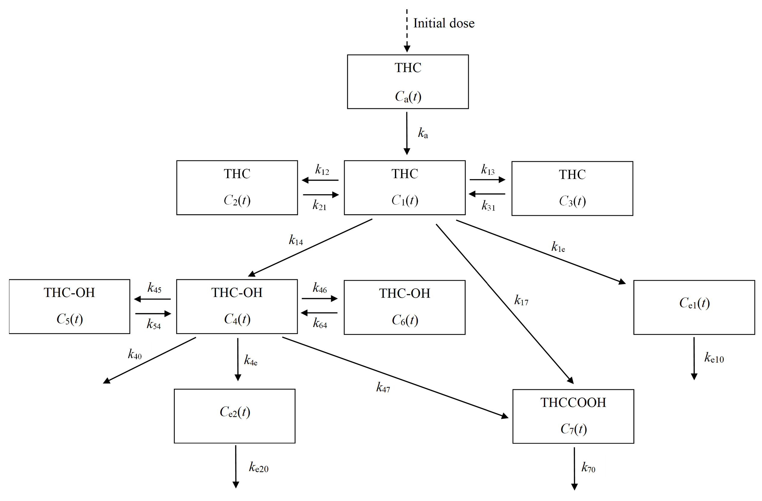
Figure 2.
The simulated THC concentration after administration of 10 mg of THC orally in each compartment: (a) in the absorption compartment; (b) in the central compartment (plasma); (c) in the rapidly equilibrating tissue compartment; (d) in the slowly equilibrating tissue compartment; and (e) in the effect site compartment.
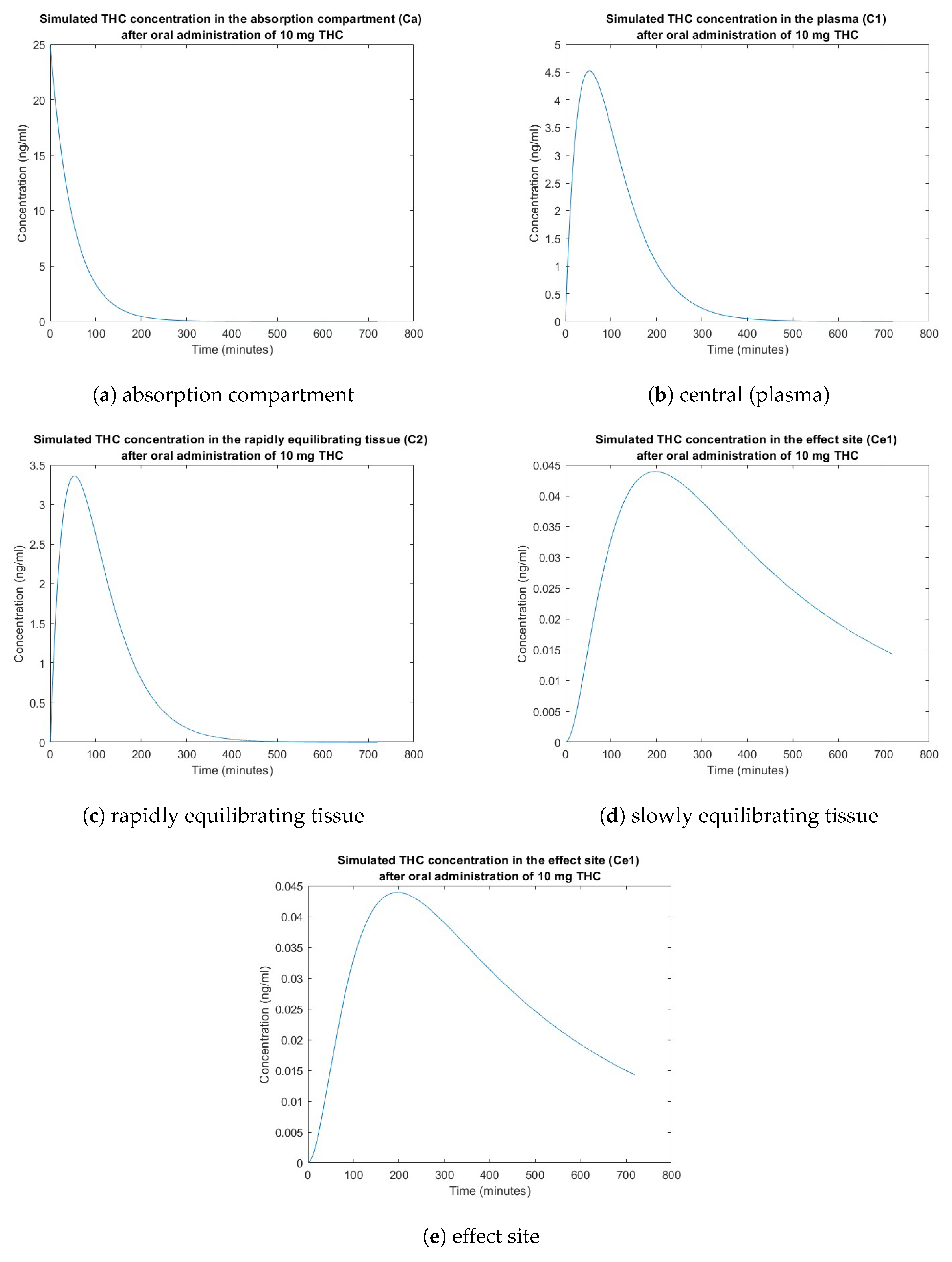
Figure 3.
The simulated THC-OH concentration after administration of 10 mg of THC orally in each compartment: (a) in the central compartment (plasma); (b) in the rapidly equilibrating tissue compartment; (c) in the slowly equilibrating tissue compartment; (d) in the effect site compartment.
Figure 3.
The simulated THC-OH concentration after administration of 10 mg of THC orally in each compartment: (a) in the central compartment (plasma); (b) in the rapidly equilibrating tissue compartment; (c) in the slowly equilibrating tissue compartment; (d) in the effect site compartment.
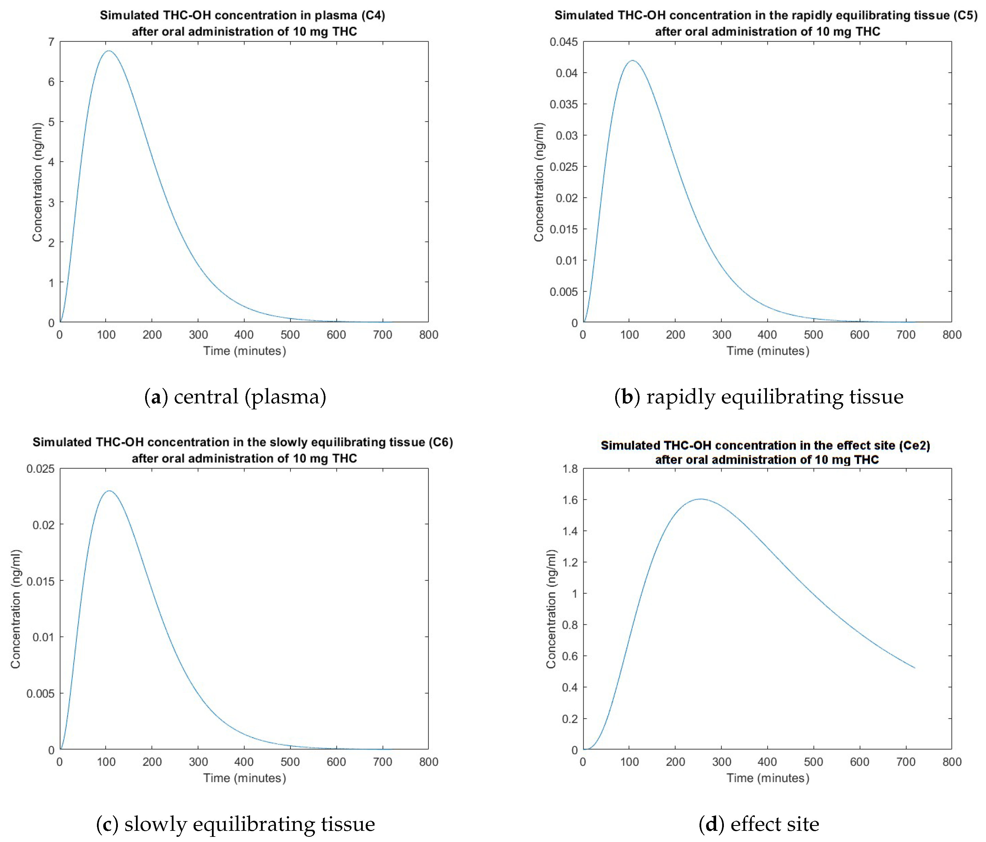
Figure 4.
The simulated THC concentration after oral administration of 10 mg of THC in each compartment.
Figure 4.
The simulated THC concentration after oral administration of 10 mg of THC in each compartment.
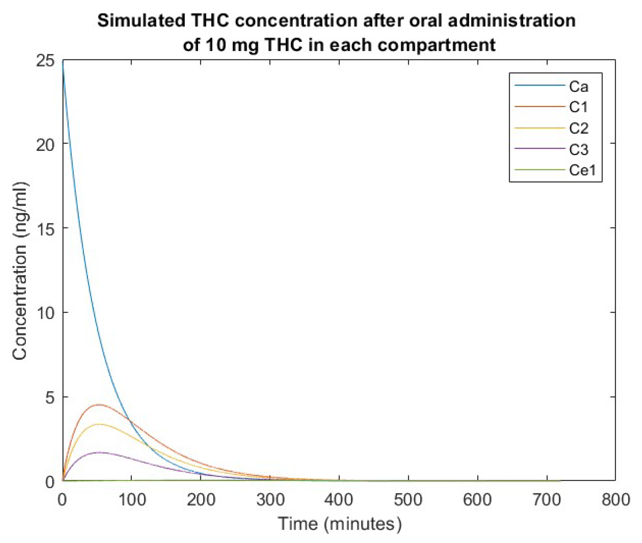
Figure 5.
The simulated THC-OH concentration after oral administration of 10 mg of THC in each compartment.
Figure 5.
The simulated THC-OH concentration after oral administration of 10 mg of THC in each compartment.
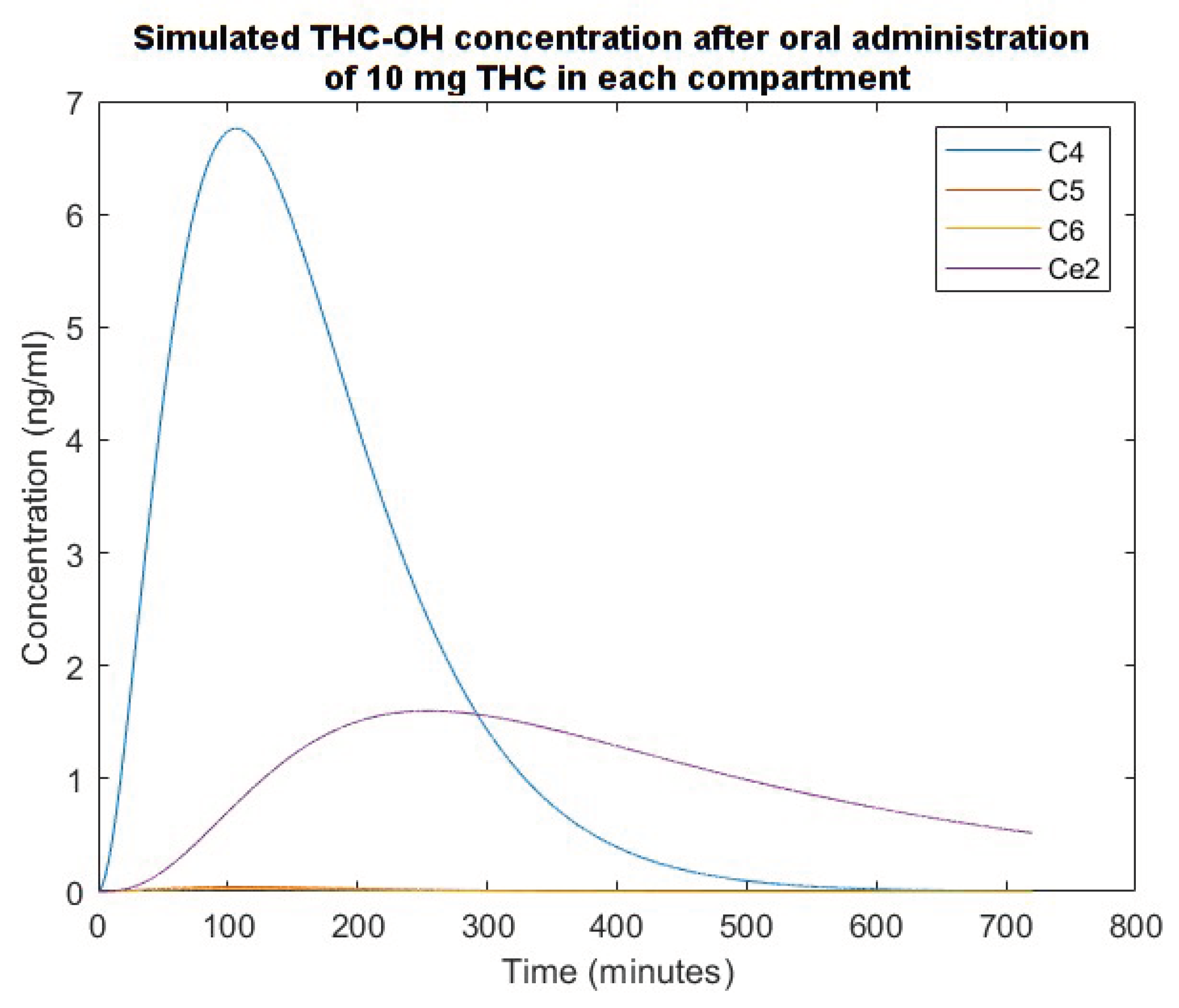

Table 1.
The estimated pharmacokinetic rate constants of THC and THC-OH after 10 mg oral administration [4].
Table 1.
The estimated pharmacokinetic rate constants of THC and THC-OH after 10 mg oral administration [4].
| Parameters | Value | Unit | Parameters | Value | Unit |
|---|---|---|---|---|---|
| 24.85 | ng/ml | 0.0001 | |||
| 0.02 | 0.0150 | ||||
| 0.7438 | 0.0062 | ||||
| 1.0000 | 1.0000 | ||||
| 0.3718 | 0.0034 | ||||
| 1.0000 | 1.0000 | ||||
| 0.0380 | 0.0015 | ||||
| 0.0001 | 0.0020 | ||||
| 0.0025 | 0.0030 |
Table 2.
Mean plasma concentration of THC and THC-OH after 10 mg THC oral administration [17].
Table 2.
Mean plasma concentration of THC and THC-OH after 10 mg THC oral administration [17].
| Time (min) | THC (ng/ml) | THC-OH (ng/ml) |
|---|---|---|
| 0 | 0.00 | 0.00 |
| 15 | 0.08 | 0.04 |
| 30 | 2.94 | 2.59 |
| 45 | 4.97 | 5.82 |
| 60 | 4.29 | 6.19 |
| 75 | 4.23 | 6.75 |
| 90 | 3.94 | 6.50 |
| 105 | 3.09 | 5.78 |
| 120 | 2.57 | 5.13 |
| 135 | 2.34 | 4.71 |
| 150 | 2.04 | 4.18 |
| 165 | 2.02 | 3.71 |
| 180 | 1.80 | 3.59 |
| 210 | 1.17 | 2.69 |
| 240 | 0.88 | 2.30 |
| 270 | 0.79 | 1.91 |
| 300 | 0.56 | 1.54 |
| 330 | 0.39 | 1.23 |
| 360 | 0.31 | 1.08 |
| 480 | 0.17 | 0.73 |
| 720 | 0.13 | 0.48 |
Disclaimer/Publisher’s Note: The statements, opinions and data contained in all publications are solely those of the individual author(s) and contributor(s) and not of MDPI and/or the editor(s). MDPI and/or the editor(s) disclaim responsibility for any injury to people or property resulting from any ideas, methods, instructions or products referred to in the content. |
© 2024 by the authors. Licensee MDPI, Basel, Switzerland. This article is an open access article distributed under the terms and conditions of the Creative Commons Attribution (CC BY) license (http://creativecommons.org/licenses/by/4.0/).
Copyright: This open access article is published under a Creative Commons CC BY 4.0 license, which permit the free download, distribution, and reuse, provided that the author and preprint are cited in any reuse.


