Submitted:
22 March 2024
Posted:
25 March 2024
You are already at the latest version
Abstract
Accurate measurement of systemic financial risk is critical to maintaining the stability of financial markets. Taking China as the subject of investigation, the Chinese Financial Stress Index (CFSI) indicator system was con-structed by integrating six dimensions and employing Gray Relation Analysis (GRA) for dimensionality reduction of the indicators. The CFSI was derived using the Attribute Hierarchy Model (AHM) method with the Criteria Importance Through the Intercriteria Correlation (CRITIC) method, and an Improved Gravitational Search Algorithm (IGSA) optimized Radial Basis Function Neural Network (RBFNN) was proposed for out-of-sample prediction of CFSI trends from 2024 to 2026. By analyzing the trend of financial pressure indicators, the relationship between financial pressure and economic activity can be effectively identified. The research findings indicate that: (1) The CFSI is capable of accurately reflecting the current financial stress situation in China; (2) The IGSA-RBFNN demonstrates good robustness and generalization capabilities, predicting that the CFSI index will reach a peak value of 0.543 by the end of 2024, and there exists a regular pattern of stress rebound towards the end of each year. The novel methodology benefits policymakers and regulatory authorities to formulate preventive measures and risk management by identifying potential risks and vulnerabilities in advance.
Keywords:
Financial stress index
; Risk prediction
; AHM
; CRITIC
; IGSA-RBFNN
1. Introduction
Due to the rapid expansion of the banking sector, financial institutions are confronted with significant pressure and challenges [1]. Simultaneously, the financial industry is intricately intertwined with the nation's real economy and exerts a profound influence on it, thereby establishing a mutually reinforcing relationship between them [2,3]. This leads to an interactive relationship [4]. The ongoing transformation of the economic development approach and structural adjustments, accompanied by moderating growth rates, have prompted the gradual recognition of previously obscured financial risks during the era of rapid expansion [5,6]. The multi-directional transmission of the shock has also inflicted significant disruptions and impairments on the tangible economy and financial system [7,8]. Hence, accurately monitoring the performance of financial markets, along with offering efficacious early warnings and systemic risk prevention measures [9,10], is pivotal to safeguarding the stability of a nation's financial markets and its real economy.
Introduced to enhance the measurement and visualization of risks within the financial system is the Financial Stress Index (FSI) [11]. This comprehensive and objective indicator captures the instability resulting from internal stresses and shocks [12], aiding national authorities in formulating fiscal policies based on an objective assessment of the current economic landscape [13,14]. Additionally, it enables financial institutions to evaluate the liquidity of the financial market and systemic risks, thereby ensuring smooth functioning of the financial system [15].
The precise forecasting of the FSI in financial markets plays a pivotal role in safeguarding the security and stability of the national financial system, as well as facilitating the steady growth of the country's real economy. The primary research methodologies employed for forecasting the FSI encompass statistical time series forecasting techniques alongside a plethora of contemporary machine learning-based forecasting approaches. Wu [16] has obtained more accurate results by combining an Auto Regressive Integrated Moving Average (ARIMA) model with a Back Propagation Neural Network (BPNN) for predictive analysis of future stress indices. Building on existing financial system risk models and taking into account the effects of time lags employed in the financial risk system, Wang et al. [17] have established a set of time-delayed financial system risk models through the analysis of the system's dynamic behavior using chaos theory. Tiwari et al. [18] analyzed the monthly data of the extracted financial stress index and the uncertainty index related to national policies, etc., and came up with the result that financial stress plays an important role in economic activities. Despite extensive discussions in previous studies on the construction and prediction of the FSI, there is still a lack of a comprehensive evaluation system for FSI and high-precision prediction model research.
The objective of this study is to propose an assignment model that integrates the Attribute Hierarchy Model (AHM) and the Intercriteria Correlation (CRITIC) coupling techniques for the development of a comprehensive FSI index. Firstly, the Gray Relation Analysis (GRA) is employed to calculate the grey integrated correlation among the constituent indicators of the FSI index, thereby assessing the strength of their relationships and eliminating redundant indicators [19]. In addition, the indicators were assigned weights using the AHM-CRITIC coupling model [20]. To construct the FSI, a method that couples subjective and objective weights is employed, facilitating the establishment of evaluation relationships between each variable through weight assignment. The Radial Basis Function Neural Network (RBFNN) under Improved Gravitational Search Algorithm (IGSA) optimization is then utilized to generate the FSI, followed by calculation of standard deviation between the generated index and original index to verify model effectiveness via IGSA-RBFNN fitting accuracy [21]. Given China's rapid economic development over the past two decades and the profound impact of the COVID-19 pandemic, the study focuses on China as its research subject. A comprehensive evaluation system for the Financial Stress Index (CFSI) is constructed, trends are predicted, and targeted preventive policy recommendations are subsequently proposed based on these findings.
The structure of this paper is as follows: In the next section, artificial neural networks and CFSI are reviewed, the process of the construction of the CFSI indicator system is given in Section 3. The CFSI measurement model of GRA-AHM-CRITIC and the IGSA-RBFNN prediction model are presented in Section 4, while the results of index construction and prediction as well as trend analysis of the CFSI are discussed in Section 5. Section 6 proposes policy recommendations for predicting the outcomes of CFSI and validates the effectiveness of the algorithm. Finally, Section 7 presents the research findings, summarizes the results, and discusses future research directions related to forecasting CFSI.
2. Literature Review
2.1. Assessment of FSI
Since Illing et al. [11] introduced the concept of financial stress, the selection of variables for constructing a stress index has received more attention. Numerous scholars have conducted a series of comprehensive studies pertaining to the selection of FSI indicators. Balakrishnan et al. [22] proposed five basic components for the construction of FSI for developing countries: sovereign debt spreads, equity market volatility, banking beta, and an exchange market stress index. Yao et al. [23] innovatively measured stress dynamics in terms of interconnectedness, and their research shows that the banking market is highly correlated with the bond market, with variables selected from banks, bonds, equities, and trading markets being constructed.
However, the majority of the aforementioned scholarly studies primarily assess stress indices based on financial markets; nevertheless, there remains an inadequate consideration of the sources of stress, which renders it susceptible to misjudging the trajectory of financial stress within said market; Therefore, Li et al. [24] suggest that the trade credit market should be taken into account as a variable in the construction of FSI for emerging markets as well as for developing countries, a component that is particularly important for the countries in the sample. As a consequence of the growing receptiveness towards global integration, local enterprises are increasingly enhancing their competitiveness and concurrently resorting to trade credit as a means of marketing their products. Therefore, this study employs external debt and trade credit as alternative measures to address the absence of the aforementioned indicator system in order to capture financial stress in the selected countries for this research. After considering the aforementioned factors, the CFSI in this study encompasses six distinct components, as detailed in Section 3.
2.2. Prediction of FSI
Considering the extensive research on constructing the FSI index, numerous dimensions have been explored in the existing literature. Li et al. [24] employed an auto-regressive model to analyze FSI from the perspective of association networks. Babar et al. [25] developed three financial stress indices using different methods, while Dai & et al. [26] built an auto-regressive model based on Granger linear causality tests for a more time-sensitive analysis. Yao et al. [27] applied asset portfolio theory to consider the impact of financial stress in submarkets on the financial system as a whole. Xu et al. [28] constructed FSI through a Markov zone transition model and developed a Time Varying Parameter-Stochastic Volatility-Vector Auto Regression (TVP-VAR) model to examine its impact on economic growth and price changes. Yang et al. [29] proposed a generalized differential decomposition model and Markov models for monitoring financial stress.
Previous studies have their merits, but often overlook the importance of considering indicator variables, which are crucial factors [30]. Insufficient variable selection may lead to inaccurate economic performance assessment, while excessive variables can complicate data processing and potentially affect analysis results due to variable interactions. Therefore, selecting and weighting indicator variables that capture financial risk from various perspectives is essential when constructing a FSI with indicators from multiple markets. Kim et al. [31] and Chen et al. [32] used different methods, such as factor analysis and principal component analysis, to extract common factors and construct FSI. Ding et al. [33] 30employed a dynamic correlation coefficient method and credit weighting method to build FSI, which is more sensitive and accurate for financial stress identification.
In conclusion, despite the utilization of diverse methodologies by numerous scholars in constructing FSI and conducting forecasting analysis, there still exist certain limitations: (1) In the process of constructing and assigning weights to FSI, indicators are extracted solely from conventional markets such as money, bonds, and stocks for construction purposes; however, the influential financial trade sector is regrettably overlooked [34,35]; (2) The process of assigning weights exhibits certain limitations. Currently, the predominant methods employed for assigning weights to financial indicator variables include principal component analysis and factor analysis, as well as portfolio theory-based analysis. However, these approaches lack clarity and stability, potentially leading to inconsistent weighting that deviates from objective facts [36,37]. Therefore, it is of paramount importance to propose a robust evaluation framework for FSI and an high-efficient forecasting model.
2.3. RBFNN in Prediction Application
Artificial neural network (ANN) is a network structure with strong self-learning and self-adaptive characteristics [38]. It possesses the capability to effectively handle non-linear fitting problems, as well as adapt to multiple samples with high proficiency. RBFNN is extensively employed in accuracy estimation and data prediction due to its utilization of radial basis functions as the activation function. Zhang et al. [39] constructed a neural network model based on a particle swarm algorithm coupled with a radial basis for estimating the accuracy of the flow layer zenith delay, and the results show that the coupled model effectively improves the estimation accuracy of the model prediction. The RBFNN model effectively enhances the precision of approximation and possesses a more streamlined structure compared to other neural networks. Simultaneously, as a feed-forward neural network, the RBFNN model possesses the capability to accurately approximate non-linear functions with arbitrary precision. This not only confers an advantage in solving non-linear fitting problems but also exhibits a faster convergence rate and enables separate learning, thereby establishing it as an ideal tool for predicting intricate phenomena. Although RBFNN demonstrates excellent performance in various prediction aspects, the challenge of parameter selection for RBFNN persists [40]. The parameters of RBFNN can be optimized using various optimization algorithms such as Particle Swarm Optimization (PSO) [41], Genetic Algorithm (GA) [42], Simulated Annealing (SA) [43], and GSA [21] for neural network training. Compared to other algorithms, GSA possesses stronger global search and parallel processing capabilities, albeit with slower training speed. Therefore, in this paper, we propose a novel three-dimensional optimization method based on GSA and construct a new IGSA-RBFNN prediction model [21]. Utilizing this IGSA-RBFNN model for FSI prediction analysis can provide valuable insights into exploring financial risks.
3. Construction of CFSI
This chapter introduces CFSI and its six components. These include Money market FSI (MFSI), Bond market FSI (BFSI), Stock market FSI (SFSI), Stock market FSI (SFSI), and Trade Credit market FSI (TCFSI), External Debt market FSI (EDFSI), and China financial market FSI (CFSI).
3.1. Money Market FSI
Money market is a venue for the movement of traded funds, and currency risk is an important component of financial stress. Interbank Spread (X11), Growth Rate of Short-Term Loans (X12), and Shanghai Interbank Offered Rate (SHIBOR) (X13) are selected to measure currency risk [16,44]. The change in X11 can reflect the impact of capital flows on currency risk; X12 can reflect the liquidity risk of banks and thus influence the pressure on the money market; X13 can facilitate the rapid development of the money market and can effectively reflect the level of activity in the money market. MFSI is defined as:
where , , denote the weights of X11, X12 and X13 in the Chinese financial market respectively.
3.2. Bond Market FSI
The risk of the bond market is also an important part of financial pressure, the financial risks in this market are often in an unstable stage during the period of economic growth, Related research based on [5,33,45]. Sovereign Bond Spreads (X21)and Negative Term Bond Spread (X22) are chosen to measure financial risk in the bond market; X21 represents the difference between the 10-year Treasury yield and the 10-year US bond yield, which is the wind vane of the debt crisis and has a sensitive response to bond market stress; X22 refers to the difference between the one-year Treasury yield and the 10-year Treasury rate, thus can affect the return of the banking sector and reflect the risk aversion in the bond market. BFSI is defined as:
where and denote the weights of X21 and X22 in the Chinese financial market respectively.
3.3. Stock Market FSI
The stock market provides a visual representation of the national economy. CSI 300 Index Yield (X31), CSI 300 Index Fluctuation Range (X32) and Stock Market Value/GDP (X33) are selected to measure equity market risk [30]. where X31 is measured using monthly stock market returns; X32 is based on a monthly stock price index; and X33 can effectively reflect stock market activity. SFSI is defined as:
where , , denote the weights of X31, X32 and X33 in the Chinese financial market respectively.
3.4. Exchange Market FSI
The foreign exchange market, as a bridge between domestic and international financial markets, is under financial stress, mostly caused by large fluctuations in exchange rates and changes in foreign exchange reserves, and is expected to become more volatile in times of financial stress. Three indicators, Yield of USD to RMB (X41), Changes in foreign exchange reserves (X42) and Vulnerability of foreign exchange market (X43), are used to quantify financial risks in the foreign exchange market [46]. Where X42 uses the change in total foreign exchange/GDP to reflect the change in foreign exchange reserves; X43 represents foreign exchange reserves/M2. EFSI is defined as:
where , , denote the weights of X41, X42 and X43 in the Chinese financial market respectively.
3.5. Trade Credit Market FSI
The stability of trade credit markets is critical to the smooth functioning of financial markets, and stress in the banking system is an important part of the financial pressure in the trade credit market [47].. Banking System Beta (X51) and Bank Index Volatility (X52) are chosen to measure financial risk in the trade credit market; where X51 is obtained by regressing the index returns of the banking system on the market returns, and X52 is based on the time-varying variance of the bank index under the Generalized Autoregressive Conditional Heteroskedasticity (GARCH) model [28], TCFSI is defined as:
where , denote the weights of X51 and X52 in the Chinese financial market respectively.
3.6. External Debt Market FSI
External debt markets are critical to the economic development of emerging economies [48]. the Growth Rate of Total External Debt (X61) is chosen as an indicator to measure the financial risk in the external debt market, and the External Debt market FSI EDFSI is defined as:
where denote the weights of X61 in the Chinese financial market respectively.
3.7. China Financial Market FSI
Based on the measurement and projection of the stress in the five financial sub-markets selected, CFSI is defined as:
where MFSI, BFSI, SFSI, EFSI, TCFSI, EDFSI represent the stress index of six financial sub-markets, namely currency, bond, equity, foreign exchange, trade credit and external debt, which are calculated by Equations (1) to (6) respectively. Specific indicators are shown in Table 1.
4. Methodology
In this chapter, a GRA-AHM-CRITIC coupling model and IGSA-RBFNN method will be introduced for the construction and prediction of CFSI. The methodology framework is shown in Figure 1.
4.1. GRA Method
GRA theory was first proposed by Professor Deng in China in the 1980s [50]. In contrast, GRA is a unified system in which each series is analyzed quantitatively to obtain the statistical set of relationships between the individual series, which in turn leads to the degree of association between the individual series [51]. If the trend of change in the two series is more similar, the higher the degree of association between these two series, and vice versa will be lower.
Due to the common trend of some economic variables and the introduction of some lagged variables, multiple cointegration will be generated, which will lead to the loss of significance of the indicator variables in the GARCH model [52], and may also lead to the failure of the prediction function of the model, thus making the prediction meaningless. Therefore, in order to solve a series of problems caused by cointegration and make the series analysis results more accurate, GRA is used to calculate the comprehensive correlation between each indicator series, and the calculation steps are as follows.
Step 1: Define the reference sequence:
where , where to the number of sequences.
Step 2: Define the contrast sequence:
Step 3: Handling of variable dimensions: In order to eliminate the influence of variable dimensions in the original data, the dimensions of the variables in each raw data series should be calculated separately and then converted into a comparable series using a standardized formula:
Step 4: Calculate the difference between the absolute value of the reference sequence and the comparison sequence:
Step 5: Calculate the correlation coefficient between the reference series and the contrast series:
where is the resolution factor, taken as 0.5 [51].
Step 6: Calculate the degree of association:
where denotes the degree of correlation between the series, the larger the value, the closer the relationship between the sequences.
4.2. Coupling Weight Calculation
4.2.1. AHM Method
AHM is a subjective assignment method. As an algorithm built on Analytic Hierarchy Process (AHP), this method has the advantages of wide application, easy calculation and consistency of testing, in addition to inheriting the advantages of AHP [53]. The specific empowerment steps for AHM are as follows:
Step 1: The weighting analysis of the evaluation indicators [54]. Satty scale is used to obtain the nth-order AHP discriminant matrix by means of expert scoring, which indicates the importance of the element i compared to the element j. AHP discriminant matrix properties are as follows:
where .
Step 2: Construction of the attribute discriminant matrix [55]. In the AHM, relative properties form the nth order attribute discriminant matrix , where the relative attribute and the scale has the transformation relation in Equation (9).
where m denotes a positive integer greater than 2.
Step 3: Calculation of relative attribute weights between each indicator. From the AHM algorithm steps, the relative attribute weight between each indicator is calculated by Equation (10):
where . n is the number of indicators, and there are .
4.2.2. CRITIC Method
CRITIC is an objective weighting method that is more objective and takes into account the influence of the size of the variation of the indicators and the conflicting nature of each other on the weights [56]. The conflicting nature of each evaluation indicator is determined based on the correlation of the indicators [57]. CRITIC's specific empowerment steps are as follows:
Step 1: Calculate the standard deviation:
where is the average of the indicators across the m programs; is the standard deviation of .
Step 2: Construct the correlation coefficient matrix:
where is the average of the schemes in index ; is the correlation coefficient between indicators and .
Step 3: Find the combined weight of each indicator :
where indicates the amount of information.
4.2.3. Lagrange's AHM-CRITIC Coefficient Coupling
After finding the subjective weights and objective weights through AHM and CRITIC, the coupling weights through the Lagrange multiplier method are calculated to reflect the relative weight relationship of each indicator and its weight share in the whole [58], the specific formula is shown in equation (20):
4.3. Prediction of CFSI by IGSA-RBFNN
4.3.1. IGSA Method
GSA is an innovative algorithm inspired by the law of gravity. In GSA, the agents are treated as objects possessing mass [21]. These agents attract one another through gravitational force, with the intensity of the force being proportional to the mass of the agents. As a result, the agent with the largest mass is assumed to occupy the optimal position. Suppose there are N agents with a d-dimensional space. The position of the i-th agent can be expressed as:
At the t-th iteration, the force acting on the i-th agent originating from the j-th agent is defined as follows:
Here, denotes the mass of the i-th agent, while represents the mass of the j-th agent. G(t) is the gravitational constant at the t-th time, is a small constant, and is the Euclidean distance between the i-th agent and the j-th agent. At the t-th iteration, the total force acting on the i-th agent is defined as follows:
where rand is a uniform random variable in the interval [0,1]. In accordance with the law of motion, the acceleration of the agent at the t-th time can be expressed as follows:
In every iteration, the velocity and position of the i-th agent are updated using the following two equations:
where rand is a uniform random variable in the interval [0,1] and and are its current position and velocity. IGSA aims to improve the gravitational coefficient, update speed formula, and position update formula of the regular GSA.
- Update of the gravitational coefficient [41]. A linear function is used to improve the gravitational coefficient, and the calculation formula can be seen in Equations (27) and (28).
- Improved velocity update. By introducing the memory function and population information sharing mechanism of the PSO algorithm [59], the GSA is improved. The improved spatial search method adopts a new strategy that not only complies with the laws of motion but also increases the memory and population information communication mechanism. The new velocity update formula is defined as shown in Equation (29):where, randi, randj, and randk are random variables in the interval [0,1]; c1 and c2 are constants in the interval [0,1]; is the best position experienced by particle i; is the best position experienced by all particles in the particle swarm. By adjusting the values of c1 and c2, the influence of gravity, memory, and population information on search can be balanced.
- Improved position update. The greedy selection mode of the differential evolution algorithm operation is adopted, as shown in Equation (30). When the fitness value of the new vector individual is better than the fitness value of the target vector individual, the newly updated individual can be accepted by the population, otherwise the individual of the previous generation will be retained in the next generation population. Among them, the fitness value of the new position is less than the fitness value of the previous generation position, and it will replace the position of the current generation individual.
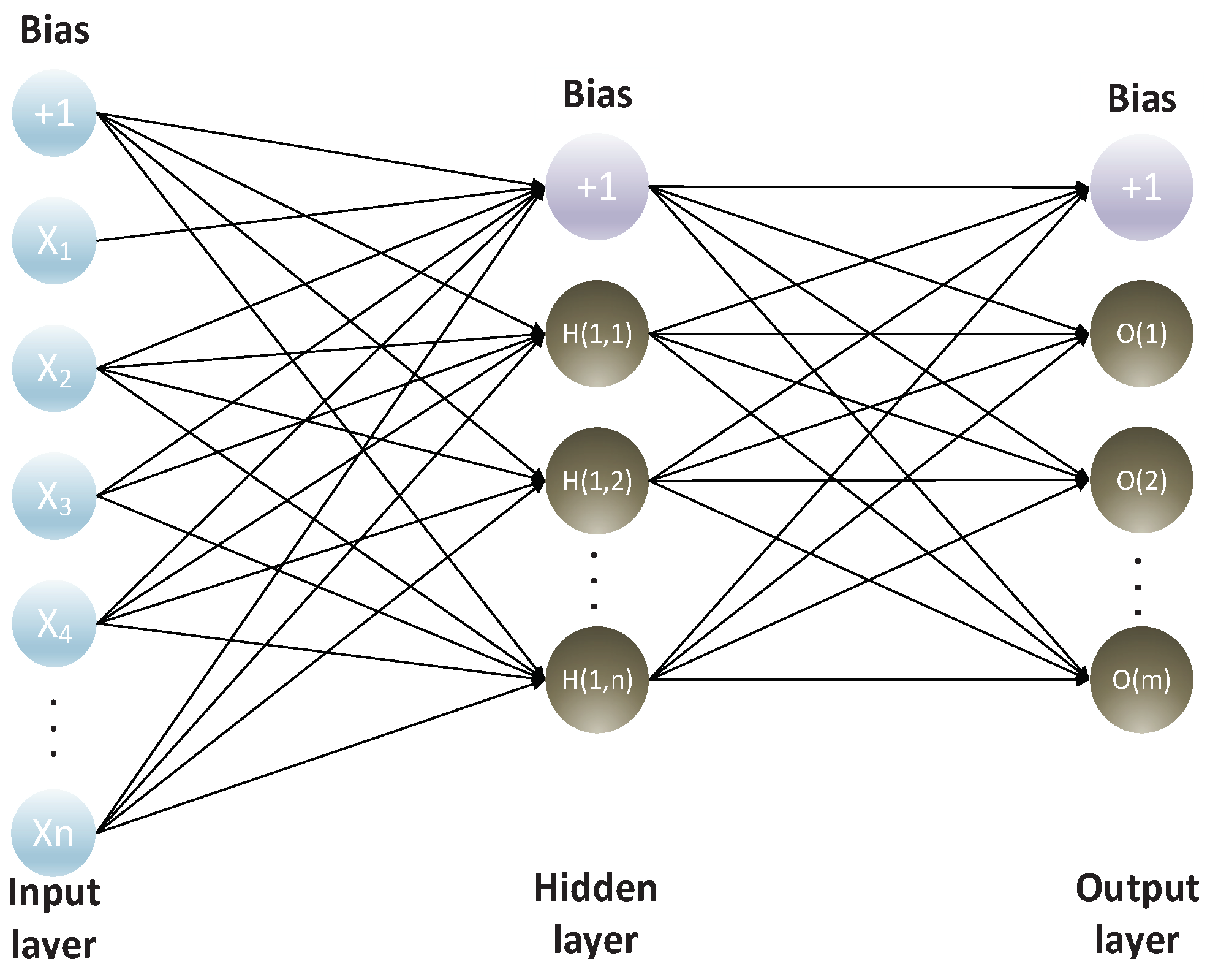
4.3.2. RBFNN Method
RBFNN is a type of feedforward neural network known for its fast learning speed and strong local approximation capability [40]. It is composed of an input layer, hidden layer, and output layer, with each output layer containing multiple neurons. Currently, RBFNN is widely applied in fields such as pattern recognition, function approximation, time series prediction, control systems [60]. The core idea is to nonlinearly map the input space to a higher-dimensional feature space, allowing the model to address problems that are not linearly separable. In the hidden layer, the output of the j-th neuron is as follows:
where as input; as the center of the j-th activation function; as the parameter controlling the degree of smoothness of the activation function; then indicates the Euclidean distance between the input and the functional center. The mapping function of the Gaussian activation function and the weighted linear summation in the common space in the output neuron of RBFNN is shown below:
where denotes the activation function of the j-th node, then denotes the weight of the j-th node.
Figure 2.
Structural of RBFNN.
4.3.3. IGSA-RBFNN Prediction Model
In the learning process of a RBFNN, three main parameters need to be determined, namely the center of the hidden layer nodes' basis functions , the width value , and the network connection weight values [40]. In the optimized prediction model of RBFNN, the key parameters in RBFNN are encoded into particles in the IGSA algorithm. The fitness value is defined as the coefficient of determination (R2) between the actual value and the predicted value [39]. The optimization is performed according to the gravitational interaction between individuals until the optimal individual is found. The optimal individual obtained from the IGSA algorithm is used to assign values to the center , width value , and network connection weight of the hidden layer nodes' basis functions in RBFNN, resulting in the IGSA-RBFNN prediction model [41]. The flowchart is shown in Figure 3.
4.3.4. Algorithm Accuracy Check
In the process of training and testing the artificial neural network, in order to obtain more accurate prediction results [61]. The Mean Square Error (MSE) is used to evaluate the error in the testing and training process of the neural network; the smaller the MSE value, the more accurate the prediction value of the neural network. The coefficient of determination R2 is used to evaluate the accuracy of the neural network in the prediction process. The range of values R2 is between [0,1], the closer the value is to 1, the higher the accuracy of the neural network fit, and vice versa; the formula is as follows:
where tj is the target value. yj is the predicted value, n is the number of data sets.
5. Result
5.1. Data Collection and Pre-Processing
Based on the WIND financial terminal, Guotaian database, People's Bank of China and other databases and websites [62], quarterly, monthly and daily data was collected for a total of 15 indicators from January 2008 to December 2021 for six financial sub-markets in China, with descriptive statistics for each indicator as shown in Table 2.
To avoid the problem of inconsistency in the scale, the indicators are first divided into two categories based on the evaluation pointers, and are standardized based on the Max-Min method. The formula is shown in equation (36):
where is the value obtained after dimensionless processing of the original data, is the actual value of the indicator. Equation (35) is used for dimensionless treatment for the forward indicator and Equation (36) for the inverse indicator.
Based on the data collected above, Equations (15) to (20) are used to carry out grey correlation analysis on the collected data in order to reduce problems such as the introduction of lagged variables and the failure of indicator prediction caused by multicollinearity [63].
Based on the GRA model constructed in Section 4.1, the grey relational matrix among various indicators is shown in Figure 4. 0.9 is set as the dimensionality reduction threshold and a P-value of 0.5 is used for significance testing [64]. It can be seen that the correlation between indicators X13 and X43 reaches 0.93; the correlation between indicators X31 and X61 reached 0.91; Delete X31 and X43 as redundancy indicators [65].
5.2. CFSI Measure
5.2.1. Calculation of AHM-CRITIC Weights
Although previous research has explored the factors of instability in global financial markets, there is still a lack of comprehensive evaluation regarding the interactions between these factors and their impact on market stress. To gain a more exhaustive perspective, we invited 15 experts with extensive backgrounds in financial risk management. This group includes 5 finance professors from renowned universities, 5 stock market experts, and 5 senior risk analysts from major global financial centers and regulatory agencies. These experts possess practical experience in areas such as financial market operations, policy formulation, asset risk assessment, and crisis response projects. By examining relevant literature on financial stress and integrating insights from these experts, we constructed a scoring matrix that covers key factors contributing to financial stress. This matrix not only reflects the impact of each factor on market stability but also elucidates their interrelations, providing a solid foundation for subsequent analysis.
The AHP discriminant matrix K (see Table 3) is constructed adopting expert scoring based on the Satty scale, subsequently converted into the attribute discriminant matrix L (see Table 4) through Equation (15). The AHP discrimination matrices for the sub-markets and the AHM attribute discrimination matrices are presented respectively in Appendix A and Appendix B. Due to the attribute discrimination matrix's consistency, construction of matrix eigenroots and eigenvectors or consistency test are not required [66]. Attribute weights for each index are determined using Equation (16), yielding the overall weighting of the AHM model.
The CRITIC weighting method is used to construct the correlation coefficient matrix through Equations (17~19), which in turn yields the weights of each indicator , and the coupling of and is calculated using Equation (14). This gives the coupling weights , the results are shown in Table 5, which denotes the result of the assignment to each sub-market, denotes the results of assigning weights to the indicators in each sub-market to which they belong, separately in each sub-market, indicates the weight of each indicator to the total market and is calculated as follows:
Table 5 shows that indicator X42 has the highest combined weighting. In the process of assigning weights to this indicator, the AHM is considered as a subjective assignment method. The foreign exchange market in which indicator X42 is located has a greater impact on the financial markets as a whole, subjective weighting is greater than objective weighting ; while indicator X13 receives the smallest combined weighting, the objective weights are higher than the subjective weights in the process of assigning weights to the indicators, and the comparison shows that the coupled weighting method can effectively weaken the effect of subjective extremes; and in the analysis of the objective weights, it can be found that there are three indicators (X11, X42 ,X61) where the coupled weight is greater than the objective weight. This is also related to the mechanism of CRITIC itself, which is conservative and does not "react" well to indicators that do not change significantly in terms of pressure, and therefore needs to be corrected with the advantage of subjective weighting.
5.2.2. Trend Analysis of FSI
The indexes are weighted according to the weights obtained from Equations (14 ~ 20) to obtain the financial stress indices of the Money market (FSI Money), Bond market (FSI Bond), Stock market (FSI Stock), Foreign Exchange market (FSI Exchange), Trade credit market (FSI Trade Credit) and External Debt market (FSI External Debt) respectively. The financial stress indexes of six sub-markets, namely FSI Trade credit, FSI External debt, and FSI China, calculated according to Equation (7), are shown in Figure 4.
According to Figure 5(a), China's money market financial risk is characterized by three stages of change: January 2010 to February 2016 is the first stage, due to the global financial crisis in 2010, resulting in money market financial stress reached a very high value of 0.049 in November 2010, then in response to the financial crisis and to ease the money market financial stress, China adopted the implementation of this policy led to a sharp decline in money market financial stress, reaching a very small value of 0.001 in February 2011, followed by an oscillating rise and reaching a maximum value of 0.09 in the first stage in June 2015; the second stage was from July 2015 to May 2017, during which money market financial risk showed a sharp decline in financial stress, reaching a maximum value of 0.09 in May 2017. The decline in financial risk during this stage can be attributed to several factors. The imposition of USA sanctions and tariffs on China in November 2016 may have exerted a stabilizing influence on the financial market [67] by incentivizing domestic production and reducing imports. Additionally, the Belt and Road Initiative (BRI) has also facilitated new investment and development opportunities in regions along its routes, thereby fostering economic growth in relevant countries and regions while potentially mitigating financial risks. Based on these findings, it is advisable to persist in implementing robust risk management strategies, encompassing the utilization of tariffs and other trade policies, to uphold financial stability. Moreover, it is imperative to diligently monitor and address any potential risks and vulnerabilities that may arise in the financial market as a result of economic events and policy changes. The third stage is from June 2017 to December 2023, where the financial risk of the money market shows frequent oscillations, fluctuating between 0.017 and 0.071.
From Figure 5(b), the financial risk of China's bond market shows three stages of change: January 2010 to June 2011 is the first stage, from 0.064 in January 2010 to 0.002 in June 2011, the reason is that the relatively safe bond market has become the "safe haven" of the nation. The second stage is from July 2011 to September 2013, during which China's bond market developed steadily and expanded, and financial stress rose sharply from 0.016 in July 2011 to 0.116 in September 2013; The surge in financial stress during this phase can be attributed to the expansion of inter-bank liquidity and the subsequent escalation in inter-bank lending rates, which might have resulted in an augmentation of financial risk within the bond market. The increased competition for funds among banks likely contributed to the adoption of risky lending practices and subsequently resulted in a surge in non-performing loans [68]. Therefore, it is imperative to persist in implementing robust risk management strategies, encompassing the vigilant monitoring and control of interbank liquidity, and adapting to fluctuations in interbank lending rates and other economic events so as to uphold financial stability. The third stage is from October 2013 to December 2023. The third stage is the period from October 2013 to December 2023, during which the financial stress in the bond market oscillates frequently, fluctuating between 0.056 and 0.121 overall.
From Figure 5(c), it can be seen that Chinese stock market financial risk shows four stages of change: January 2010 to October 2010 is the first stage, during this interval due to the 2010 financial crisis, stock market financial stress rose sharply, reaching an extreme value of 0.18 in October 2010 in this interval; November 2010 to June 2016 is the second stage, during which the stock market gradually regained stability and stock market financial stress continued to oscillate, fluctuating between 0.072 and 0.148 overall; the third stage, from July 2016 to April 2017, during which the Chinese stock market was in the doldrums and stock market financial stress declined sharply, from 0.106 in July 2016 to 0.037 in April 2017. The occurrence of Brexit has instigated a state of uncertainty in the global market, encompassing apprehensions regarding international trade relations [69]. This prevailing ambiguity may prompt investors to exercise prudence in light of an indeterminate future, consequently exerting a detrimental influence on financial markets such as the Chinese stock market. Moreover, the adjustment of the United States' tariff policies towards China has led to an escalation in tariffs between the two nations, triggering a ripple effect in the global economy. The aforementioned pressure has exerted an impact on Chinese export businesses and manufacturing, thereby augmenting uncertainty within the global supply chain and precipitating a decline in the profitability of certain companies, consequently leading to a downturn in stock market performance. In such circumstances, investors tend to gravitate towards safer haven assets, thus contributing to risk diversification within financial markets and mitigating portfolio volatility. May 2017 to December 2023 is the third stage, during which stock market financial stress oscillates frequently, fluctuating between 0.044 and 0.138 overall.
According to Figure 5(d), China's foreign exchange market financial risk shows an overall oscillating upward trend, with a sharp rise in financial stress in the foreign exchange market at the beginning of each year due to economic recovery and a strong and slight rise in the external exchange rate; after this period, due to a slowdown in economic growth and a narrowing of external spreads; In response to the economic cycle, enterprises and investors may exhibit an increased demand for foreign exchange at the onset of a new year, thereby contributing to market volatility. When economic growth decelerates, the external interest rate spread contracts, potentially alleviating financial strain. Additionally, heightened external interest rates can exert increased financial pressure on the foreign exchange market [57], particularly for enterprises that rely on borrowing in foreign currencies. The fluctuations in the global economy have a direct impact on the dynamics of the foreign exchange market. Due to the impact of the COVID-19 pandemic, the deceleration of the global economy has engendered apprehensions regarding exchange rates, thereby exacerbating uncertainty in the foreign exchange market. These intertwined factors give rise to a multifaceted scenario wherein overall financial risk in the foreign exchange market exhibits an oscillating upward trajectory. At the end of the year, the market operates smoothly and financial pressure fluctuates less. During the time interval from January 2010 to December 2023, from 0.194 in January 2010 to 0.174 in December 2023.
According to Figure 5(e), the financial risk of China's trade credit market shows three stages of changes: January 2010 to July 2016 is the first stage, during which the financial stress of the trade credit market oscillated down and reached a very small value of 0.018 in July 2016 for this period; August 2016 to July 2017 is the second stage, during which the trade credit market showed a significant upward trend. The United Kingdom's decision to leave the European Union in June 2016 led to a surge in global market uncertainty, with the progress and uncertainties surrounding Brexit negotiations exacerbating financial market volatility [69]. Consequently, this had an impact on the trade credit risks faced by multinational corporations. Additionally, in early 2017, the United States implemented a series of trade sanctions against China, sparking trade tensions between the two nations. This could have led to an increase in financial risk in the trade credit market, affecting trade financing and credit conditions for businesses. The U.S.-China trade dispute and Brexit have introduced a level of uncertainty into the global economy and trade system, exerting a direct impact on the trade credit market and reflecting the prevailing atmosphere of tension and unpredictability in global trade. The third stage is from August 2017 to December 2023, during which the financial risk in the trade credit market oscillates frequently, fluctuating between 0.013 and 0.079 overall.
According to Figure 5(f), the financial risk in China's external debt market shows three stages of change: January 2010 to November 2016 is the first stage, during which the trend of financial stress in the external debt market is relatively stable; December 2016 to April 2017 is the second stage, during which the financial risk in the bond market first rises sharply and reaches a very large value of 0.45 in January 2017, after which it falls sharply and reaches a very small value of 0.06 in April 2017. Due to the United States implementing a series of trade sanctions against China in early 2017, it heightened the trade tensions between the U.S. and China. This likely contributed to an increase in financial risk in the bond market [70], particularly in bonds related to U.S.-China trade relations. Additionally, the uncertainty surrounding the Brexit negotiations may have exerted an impact on the bond market during this period. Concerns regarding the post-Brexit UK economy and financial markets might have prompted investors to reevaluate bonds, thereby inducing fluctuations in financial risk. The significant surge and subsequent rapid decline in financial risk observed in the bond market during this period may suggest a high degree of market sensitivity to these events. It is possible that there were instances of market overreactions or short-term hedging actions by participants due to uncertainties surrounding the subsequent developments of these events. May 2017 to December 2023 is the third stage, during which the financial risk in the bond market shows a relatively stable trend of 0.06. The third stage is from May 2017 to December 2023, during which the financial risk in the bond market shows a relatively stable trend.
According to Figure 5(g), the characteristics of China's financial market risk show three stages of change: January 2010 to February 2016 is the first stage, during which China's financial stress rose sharply and reached a very high value of 0.55 in February 2016; March 2016 to May 2017 is the second stage, during which China's financial stress index fell sharply and reached a very high value of 0.27. The third stage is from May 2017 to December 2023, during which China's financial market risk rises sharply and reaches a very high value of 0.42 in September 2023; except for this, in each year, China's financial market risk shows an increase followed by a decrease, rising sharply at the beginning of the year and then falling sharply thereafter.
These three stages indicate that despite the rapid and high-quality development of China's financial market, the potential risks and crises have been intensifying dynamically over the past decade [62]. In the initial phase (January 2010 to February 2016), the financial market faced significant pressure due to repercussions from the global financial crisis and China's economic structural adjustments. This period witnessed sharp market fluctuations and increased pressure, indicating potential risks. The second stage (March 2016 to May 2017) may potentially reflect the favorable impacts of a series of macro-prudential policies and financial market reforms implemented by the Chinese government. The implementation of these policies might have contributed to mitigating financial risks and fostering market stability. The third stage (May 2017 to December 2023) may be subject to external influences, such as global economic uncertainty and trade tensions. This implies that China's financial market is confronted with emerging potential risks in the recent period, necessitating heightened vigilance, monitoring, and responsive measures. Over the past decade, China's financial market has undergone various stages of risks and crises, influenced by both global and domestic factors. The government has implemented effective policy measures to mitigate financial pressures corresponding to different economic conditions during diverse periods. Continued emphasis on monitoring global economic conditions and trade dynamics is strongly recommended. Moreover, it is imperative to prioritize timely and adaptable policy responses to effectively address potential emerging economic and financial challenges.
5.3. FSI Prediction and Trend Analysis
After constructing the CFSI and its component indices, to predict the financial stress index for a future period, predictions are carried out on the MATLAB platform with a time step of one month, inferring the fluctuations of each index over the next 48 periods. The number of IGSA-RBFNN neurons in the hidden layer is set to automatically iterate between 10 and 100, the learning rate is set to 0.1, number of iterations is set to 1000, and the L2 regularization rate is set to 1.0. In IGSA optimization algorithm, the number of iterations is 150, c1=0.15, c2=0.25, G0=100, and is 20. In addition, the RBF activation function and the Limited-memory Broyden Fletcher Goldfarb Shanno (L-BFGS) solver are used for computation [71]. Two evaluation metrics, R2 and MSE, was employed to test the model performance.
The forecast results for 2024 to 2026 were obtained by forecasting the financial stress index of six financial market segments in China and the FSI of the total financial market in China through IGSA-RBFNN, as shown in Figure 4(a) to Figure 4(g). The R2 and MSE average levels are 0.9542 and 0.00023, respectively, indicating that the prediction model based on IGSA-RBFNN has good robustness and generalization performance, suggesting that the prediction results are highly reliable.
According to Figure 6(a), China's money market faces three distinct phases of future financial risk. The first phase, from January 2024 to June 2024, shows a significant increase in risk, indicating potentially volatile economic conditions. This risk rises from 0.039 in January 2024 to 0.052 in June 2024, suggesting the need for heightened vigilance and potential adjustments to risk management strategies by market participants. The second stage spans from July 2024 to January 2025 and represents a period of stabilization in the market. Investors and regulators should utilize this phase wisely by implementing precautionary measures [10] such as enhancing liquidity buffers or reevaluating interest rate policies to mitigate any upcoming risks. The third stage, lasting from February 2025 to February 2026, is characterized by frequent oscillations in financial risk levels. In December 2025, the financial risk reaches its peak at 0.052, followed by significant fluctuations ranging between 0.005 and 0.058 from January 2026 to December 2026.This persistent volatility necessitates a comprehensive review of current investment portfolios and the adoption of more robust hedging techniques to safeguard against unforeseen shifts in the market.
The financial risk trajectory of China's bond market, as shown in Figure 6(b), goes through three distinct stages. Initially, from January 2004 to October 2024, the bond market experiences an oscillating yet ascending pattern of financial risk, increasing from 0.069 in November 2024 to 0.093 in October 2024. This period is marked by high volatility within the market, indicating a need for increased scrutiny from regulators and investors to prepare for potential adjustments and establish strong risk management protocols [52], reinforcing market confidence and curbing speculation. In the second stage from November 2024 to May 2025, there is a noticeable decline in financial risk, decreasing from 0.083 to 0.077. This significant drop offers cautious optimism for policy adjustments and investment opportunities. During the final stage from June 2025 to December 2026, the bond market experiences frequent fluctuations in financial risk, ranging between 0.073 and 0.105. This uncertain period highlights the potential impact of both domestic and international developments on market stability. Market participants should utilize this phase to evaluate their risk diversification strategies and operational frameworks' responsiveness to sudden shifts, strengthening financial security amidst continuous market changes.
The projected stages of financial risk in China's stock market, as shown in Figure 6(c), indicate a nuanced trajectory over the next three years. In the initial phase (January 2024 to July 2024), there is a gentle downtrend in financial risk from 0.121 to 0.091. This decline suggests relative stability and reflects positively on current financial policies and risk management practices, which should be maintained and possibly reinforced for sustained positive momentum. During the second stage from August 2024 to October 2025, the stock market experiences increased volatility, with fluctuations mainly ranging between 0.081 and 0.099. Measures like improved market surveillance, real-time monitoring of macroeconomic indicators, and responsive policy frameworks could be considered to manage unpredictable swings and boost investor confidence. The final stage, spanning from November 2025 to December 2026, sees a gradual decline in financial risk, reaching 0.073 by the end of this period. This descent suggests market mechanisms maturing and investors adapting to earlier regulatory measures. Leveraging predictive analytics advancements could help preempt risk factors and formulate strategies.
According to Figure 6(d), in the initial phase from January 2024 to October 2025, there is a gradual decline in financial risk, signaling stabilization with a decrease from 0.237 to 0.157. This could be attributed to effective regulations and a favorable global economy. The subsequent period, from November 2025 to February 2026, witnesses a sharp increase in financial risk levels, with the risk soaring back to its peak of 0.237. This surge may reflect the market's response to unexpected internal or external shocks like geopolitical tensions, sudden economic policy shifts, or global market volatility. It emphasizes the need for robust contingency plans and flexible monetary policies that can swiftly respond to sudden financial stress. In the final stage, from March 2026 to December 2026, the financial risk in the foreign exchange market sharply declines to 0.171. This reduction may indicate successful implementation of mitigation strategies and adaptive mechanisms by the market to handle the mentioned shocks.
According to Figure 6(e), China's trade credit market financial risk is expected to undergo a three-phase evolution in the near future. The initial phase, from January 2024 to May 2025, shows a gradual increase in financial risk, with the trade credit market risk index rising from 0.037 to 0.056. This suggests relative stability but calls for cautious monitoring to prevent any disruptive escalation that could impact market confidence. The second phase, from June 2025 to November 2025, sees a sharp increase in the risk index, reaching a peak of 0.067. Strengthened oversight, including closer scrutiny of trade credit transactions and adherence to strict credit standards, could be crucial in preventing potential defaults caused by excessive leverage. The final stage, from December 2025 to December 2026, is characterized by frequent oscillations in financial risk levels ranging from 0.023 to 0.041. This period of volatility emphasizes the need for robust risk management frameworks and sufficient market liquidity to absorb shocks. Exploring diversification of trade finance products across sectors and regions can also help distribute risk more evenly.
According to Figure 6(f), the financial risk of China's external debt market is characterized by three stages of change. In the first stage, from January 2024 to October 2025, the financial risk of the external debt market shows a slow decline, from 0.009 in January 2024 to 0.007 in October 2025, it is still a crucial period for maintaining the stability of the external debt market. In the second stage, from November 2025 to April 2026, the financial risk of the external debt market shows a sharp increase, climbing from 0.008 in January 2025 to 0.012 in April 2026. The rise in financial risk may be linked to economic uncertainty and changes in global politics. To reduce these risks, we suggest improving external debt transparency, promoting international financial stability through increased cooperation among nations [13]. In the third stage, from May 2026 to December 2026, the financial risk in the external debt market shows a sharp decrease, falling from 0.012 in April 2026 to 0.01 in December 2026. The sharp decline in financial risk may create potential opportunities for external debt investment. It is recommended to optimize the structure of external debt investments, diversify the portfolio, and promote the healthy development of the external debt market.
According to the analysis of Figure 6(g), China's financial market risk is expected to undergo four stages of change. In the first stage from January 2024 to November 2024, the overall financial market risk is predicted to exhibit a substantial decline from 0.548 in January 2024 to 0.421 in November 2024, followed by a short period of fluctuation. Financial institutions should capitalize on favorable market conditions to bolster their capital, strengthen risk management capabilities, and prepare for potential increases in financial risks in subsequent stages [45]. The second stage runs from December 2024 to February 2025, during which the financial market risk is projected to increase rapidly from 0.426 in December 2024 to 0.543 in February 2025. Financial institutions should adopt a cautious investment approach and avoid excessive borrowing to minimize credit default risks. The third stage spans from March 2025 to September 2026, where the financial market risk is expected to rise sharply from 0.548 in January 2024 to a peak of 0.53 in September 2026 with a slow upward trend. The regulators should enhance market surveillance, closely monitor financial institutions' behavior, and introduce macroprudential measures to prevent systemic risks. The fourth stage occurs from October 2026 to December 2026, where the financial market risk is forecast to experience a significant drop from 0.530 in October 2026 to 0.467 in December 2026. It is crucial to promptly and effectively implement support measures, such as injecting liquidity, to stabilize financial markets and promote sustained economic growth.
6. Conclusion and Prospect
6.1. Conclusions and Suggestions
Despite the absence of evident indications of severe financial crises, the ongoing transition process towards a market economy remains incomplete within the context of still developing emerging markets. The disparities in the reform of local and global financial systems give rise to significant financial volatility, underscoring the imperative for establishing a timely FSI. The sub-indices derived from the analysis conducted in this study demonstrate how market volatility and uncertainty can potentially impact the overall market dynamics, particularly during economic downturns, thereby influencing long-term growth trends. The predictive efficacy of the financial stress index has been empirically validated, thereby enabling proactive measures to prevent adverse financial events and facilitating timely interventions. The research findings suggest that factors inherent in transitional systems may give rise to significant financial volatilities, potentially precipitating subsequent financial crises. Therefore, based on the comprehensive evaluation and prediction results of the CFSI as well as studies on relevant major financial events, specific recommendations are proposed.
- Building a timely risk warning system is key to curbing systemic risks in financial markets. Despite the presence of sufficient qualitative analysis on such risks, there is a noticeable dearth of quantitative analysis and mathematical support [72]. The insufficiency is also apparent in the imperfect mechanisms for early warning of financial risks. As evidenced by the forecast results of CFSI, there is a gradual and consistent increase in CFSI from 2024 to 2026. Therefore, it is imperative to develop dedicated early warning models in order to enhance the resilience level of systemic risks.
- The interplay among financial subsystems can engender instability in the overall market. For instance, the financial risk of the Chinese bond market rose from 0.064 in 2010 to 0.002 in 2011 and then increased to 0.116 during a stable expansion period. According to model predictions, bond financial risk is expected to fluctuate between 0.073 and 0.105 from 2024 to 2026. Moreover, the risk level in the money market over the past few years has risen from a low of 0.001 to a peak of 0.071 and is likely to oscillate between 0.052 and 0.058 during the period from 2024 to 2026. Therefore, it is imperative to enhance the scope, frequency, and quality of microeconomic financial data collection in order to effectively mitigate risk propagation across multiple subsystems and aggregate statistical risk indicators, thereby safeguarding investor interests.
- The ongoing financial reform in China is gradually adapting to the transformation of its economic structure, exemplified by measures implemented in special economic zones as well as agricultural and industrial reforms. However, these reforms are not closely aligned with global financial issues, potentially resulting in distortions within the pricing structure of capital markets and an escalation of stability risks within the financial system. Running through the financial system reforms is the foreign exchange market, which fluctuated from 0.194 in 2010 to 0.174 in 2023. The projected pace of reform is expected to raise this figure to 0.237 in 2024 and then decrease to 0.171 by the end of 2026. China should carefully calibrate the pace and extent of its reforms to ensure a seamless transition of the financial system, while striking an optimal equilibrium between fostering long-term reforms and maintaining stability.
- Given the extensive experience of the international P2P lending model, it is imperative to reevaluate the issue of 'rigid redemption' in the Chinese market and implement prompt measures for its resolution. The liquidity challenges arising from inflexible redemption policies need to be prioritized, as a significant portion of funds are being drawn towards net lending, while the real sectors struggle to secure adequate financing for their growth [73]. For example, the risk in the external debt market peaked at 0.45 in January 2017 but then fell to 0.06 in April of the same year. Forecasts show that this market will remain relatively stable from 2024 to 2026. Therefore, it is imperative to eliminate the policy of "principal and interest guarantee" for P2P lending products and guide investors towards enhancing their risk awareness. This will enable investors to assume the risks themselves, thereby alleviating the burden on the entire online lending industry.
6.2. Comparison Analysis
To better illustrate the robustness and generalization performance of the IGSA-RBFNN algorithm in CFSI, this study selects algorithms such as Multi-Layer Perceptron Neural Network (MLPNN), RBFNN, Light Gradient Boosting Machine (LightGBM), and GSA-RBFNN for algorithm comparison, which are used for parameter accuracy testing. The accuracy of each algorithm in terms of MSE and R2 results is shown in Figure 7 and Figure 8.
The collected data were trained using five different algorithms to test the accuracy on CFSI, MFSI, BFSI, EFSI, TCFSI, and FDFSI. According to Figure 7 and Figure 8, it is concluded that the IGSA-RBFNN algorithm has an average MSE of 0.0002 and an average R2 of 0.9629. Meanwhile, the MSE results obtained from the LightGBM, MLPNN, and RBFNN algorithms fluctuate between 0.0009 to 0.0026, with R2 results fluctuating between 0.9383 to 0.9513. The average MSE and average R2 of the GSA-RBFNN algorithm are 0.0009 and 0.9547, respectively.
Comparing the accuracy testing results of each algorithm indicates that the precision tests conducted on the IGSA-RBFNN algorithm are superior to other algorithms, followed by GSA-RBFNN. The accuracy testing results of the LightGBM, MLPNN, and RBFNN algorithms are slightly inferior. This suggests that the IGSA-RBFNN algorithm exhibits better robustness and applicability to the mechanisms influencing financial risk and indices of financial risk, reflecting superior predictive performance, generalization capabilities, and resistance to overfitting compared to similar algorithms.
7. Conclusion and Prospect
7.1. Conclusions
The systematic method of constructing and calibrating financial system stress measurement for the CFSI measurement process is explained. The CFSI plays a pivotal role in the surveillance of financial risk in China, offering an effective approach to employing financial instruments for gauging the stress on the financial system. The outcomes of this stress measurement reflect the relative contributions of individual indicators towards overall pressure; from an economic policy perspective, the implementation of economic measures during periods of financial stress is contingent upon the underlying cause of the stress. If the primary source of financial strain lies within the bond market, it becomes imperative for economic policies to prioritize bolstering and fortifying this particular market segment. The measurement of financial stress is thus valuable in assisting policymakers to formulate appropriate economic policies for addressing financial risks. The primary conclusions are as follows:
(1) In the process of measuring the CFSI, we meticulously considers the unique characteristics of China as a developing nation and comprehensively explores the information quality of each indicator. The final CFSI encompasses six major market segments: currency, bond, stock, foreign exchange, trade credit, and foreign debt markets. Additionally, it evaluates the overall financial risk in China and its associated risks within these six major segments. The financial stress between 2010 and 2023 basically shows three stages of change, with financial stress shaking out and rising from January 2010 to February 2016, falling sharply from March 2016 to May 2017, and rising sharply from May 2015 to December 2023; the overall financial risk is at a relatively high.
(2) In the process of forecasting the CFSI, the IGSA-RBFNN is used to forecast the financial stress index for the years 2024 to 2026. Additionally, the MSE is employed to test the accuracy of the algorithm, ensuring the validity of the forecast results. The forecast results show that the overall financial market and six major market segments in China have a lower level of financial risk from July 2025 to January 2026 compared with other periods, while the Chinese financial system is in a long-term high stress stage from January 2026 to August 2026, indicating that economic activities are relatively frequent during this period.
7.2. Limitations and Future Work
This article employs the GRA, AHM-CRITIC and IGSA-RBFNN model to conduct out-of-sample predictions of the CFSI, with the objective of accurately assessing China's systemic financial risks, which play a pivotal role in maintaining stability within the Chinese financial markets. However, it is imperative to address certain limitations in future research endeavors.
(1) In the GRA, the correlation between indicators is mitigated by implementing a stringent correlation coefficient threshold of 0.9. The selection of different thresholds may have an impact on the final outcomes, and future investigations could conduct additional sensitivity analyses to ascertain the optimal threshold.
(2) For the long-term prediction of CFSI trends, there exist numerous uncertainties encompassing political, economic, and social dynamics that may potentially impede the precision of the model. The proposed forecasting model is based on sample data from 2010 to 2023, used to predict the trends of the CFSI for the next 48 months. The model has a certain timeliness, and can be developed into a dynamic forecasting model with subsequent new data.
(3) Although this article presents the effective prediction of FSI using IGSA-RBFNN, it lacks empirical research on the dynamic relationship between financial risk factors. In the future, additional utilization of Structural Equation Modeling (SEM), System Dynamics Method (SDM) [74,75], and other systems theory models can be employed to explore the generation and dynamic evolution analysis of financial stress in order to achieve efficient risk prediction and control.
Author Contributions
Y.T.: conceptualization; funding acquisition; project administration; writing review and editing. Y.W: investigation; writing review and editing; resources.
Funding
This work is supported by Wuhan Urban Construction Bureau Science and Technology Plan Project, grant number: 202238, and supported by the project from the Wuhan University of Technology Campus level Research Project, grant number: 20221h0128.
Institutional Review Board Statement
Not applicable.
Informed Consent Statement
Not applicable.
Data Availability Statement
On behalf of all the authors, the corresponding author states that our data are available upon reasonable request.
Conflicts of Interest
The authors declare no conflict of interest.
Appendix A

Table A1.
Determination of the judgment matrix X1.
| X11 | X12 | X13 | |
| X11 | 1 | 1/3 | 1/5 |
| X12 | 3 | 1 | 1/2 |
| X13 | 5 | 2 | 1 |
Table A2.
Determination of the judgment matrix X2.
| X21 | X22 | |
| X21 | 1 | 3 |
| X22 | 1/3 | 1 |
Table A3.
Determination of the judgment matrix X3.
| X32 | X33 | |
| X32 | 1 | 3 |
| X33 | 1/3 | 1 |
Table A4.
Determination of the judgment matrix X4.
| X41 | X42 | |
| X41 | 1 | 3 |
| X42 | 1/3 | 1 |
Table A5.
Determination of the judgment matrix X5.
| X51 | X52 | |
| X51 | 1 | 1/5 |
| X52 | 5 | 1 |
Appendix B
Table B1.
Determination of the attribute discrimination matrix X1.
| X11 | X12 | X13 | |
| X11 | 0 | 1/7 | 1/11 |
| X12 | 6/7 | 0 | 1/5 |
| X13 | 10/11 | 4/5 | 0 |
Table B2.
Determination of the attribute discrimination matrix X2.
| X21 | X22 | |
| X21 | 0 | 6/7 |
| X22 | 1/7 | 0 |
Table B3.
Determination of the attribute discrimination matrix X3.
| X32 | X33 | |
| X32 | 0 | 6/7 |
| X33 | 1/7 | 0 |
Table B4.
Determination of the attribute discrimination matrix X4.
| X41 | X42 | |
| X41 | 0 | 6/7 |
| X42 | 1/7 | 1 |
Table B5.
Determination of the attribute discrimination matrix X5.
| X51 | X52 | |
| X51 | 0 | 1/11 |
| X52 | 10/11 | 0 |
References
- Al-Fayoumi, N.; Abuzayed, B.; Arabiyat, T.S. The banking sector, stress and financial crisis: Symmetric and asymmetric analysis. Appl Econ Lett 2019, 26, 1603–1611. [Google Scholar] [CrossRef]
- Koomson, I.; Churchill, S.A.; Munyanyi, M.E. Gambling and Financial Stress. Soc Indic Res 2022, 163, 473–503. [Google Scholar] [CrossRef]
- Chiba, A. Financial Contagion in Core–Periphery Networks and Real Economy. Comput Econ 2019, 55, 779–800. [Google Scholar] [CrossRef]
- Chen, X.; Hao, A.; Li, Y. The impact of financial contagion on real economy-An empirical research based on combination of complex network technology and spatial econometrics model. PLoS ONE 2020, e0229913. [Google Scholar] [CrossRef] [PubMed]
- Keda, W. Research on the Construction of Financial Stress Index and Its Macroeconomic Effects. Shanghai Finance 2020, 30–38. [Google Scholar] [CrossRef]
- Wen, Z. China's Growth Accounting Based on Binary Structure: Theoretical and Empirical Analysis of Introducing Labor Employment Rate. Social Sciences in China 2023, 39–58. [Google Scholar]
- Huang, X.; Guo, F. A kernel fuzzy twin SVM model for early warning systems of extreme financial risks. Int J Financ Econ 2021, 26, 1459–1468. [Google Scholar] [CrossRef]
- Cheng, L.; Yanting, Z. A Study on the Linkage of Leverage Ratio, Real Estate Prices, and Financial Risks in Various Sectors of the Real Economy. Financial Regulation 2021, 92–114. [Google Scholar] [CrossRef]
- Hang, Y. Construction and Analysis of China's Systemic Financial Risk Stress Index. Western Finance 2019, 38–42. [Google Scholar] [CrossRef]
- Ahamed, M.M. Inclusive banking, financial regulation and bank performance: Cross-country evidence. J Bank Financ 2021, 124, 106055. [Google Scholar] [CrossRef]
- Illing, M.; Liu, Y. Measuring financial stress in a developed country: An application to Canada. J Financ Stabil 2006, 2, 243–265. [Google Scholar] [CrossRef]
- Lixun, Y.; Jiayi, L.; Shangshi, M. China Financial Stress Index and Monitoring Efficiency Evaluation. Shanghai Economic Research 2024, 106–120. [Google Scholar] [CrossRef]
- Zhongming, T.; Xiao, W.; Sumin, Y. Research on the Cross Market Transmission of Systemic Financial Risks Based on Stress Index. Economic Forum 2023, 139–152. [Google Scholar]
- Duoqi, X. On the Regulatory Failure and Tax Regulation of Systemic Financial Risks. Political and Legal Theory Series 2023, 14–28. [Google Scholar]
- Cevik, E.I.; Dibooglu, S.; Kenc, T. Financial stress and economic activity in some emerging Asian economies. Research in international business and finance 2016, 36, 127–139. [Google Scholar] [CrossRef]
- Guanglei, W.; Xiaotai, W.; Bin, W. Analysis of the impact of the COVID-19 on China's systemic financial risks: Based on the financial stress index and portfolio model. Management modernization 2021, 41, 103–107. [Google Scholar] [CrossRef]
- Wang, H.; Liu, R.; Zhao, Y.; Du, X. Prediction and Application of Computer Simulation in Time-Lagged Financial Risk Systems. Complexity 2021, 2021, 1–10. [Google Scholar] [CrossRef]
- Tiwari, A.K.; Nasir, M.A.; Shahbaz, M. Synchronisation of policy related uncertainty, financial stress and economic activity in the United States. International journal of finance and economics 2021, 26, 6406–6415. [Google Scholar] [CrossRef]
- Li, J.L.J.; Wang, M.W.M. How modern financial support drives innovative urban planning and construction: Grey relation analysis(Article). Open House Int 2018, 118–123. [Google Scholar] [CrossRef]
- Liu, B.; Dong, L.; Fan, R. in Research on the financial risk measurement and prediction of small and medium-sized enterprises based on the artificial neural network under AHM-CRITIC coupling, 2022 International Conference on Agriculture, Forestry and Economic Management (AFEM 2022), 2022; 2022.
- Hardiansyah; Salim, A.; Hadimi; Irman. Hybrid PSO-GSA Applied To Dynamic Economic Dispatch With Prohibited Operating Zones. IOSR journal of electrical and electronics engineering 2019, 10–17. [Google Scholar]
- Balakrishnan, R.; Danninger, S.; Elekdag, S.; Tytell, I. The Transmission of Financial Stress from Advanced to Emerging Economies. Emerging markets finance & trade. [CrossRef]
- Yao, X.; Le, W.; Sun, X.; Li, J. Financial stress dynamics in China: An interconnectedness perspective. Int Rev Econ Financ 2020, 68, 217–238. [Google Scholar] [CrossRef]
- Shaofang, L.; Xiaoxing, L. Financial System Pressure: Exponential Measurement and Spillover Effects Research. Systems Engineering-Theory & Practice, 2020; 40, 1089–1112. [Google Scholar]
- Babar, S.; Latief, R.; Ashraf, S.; Nawaz, S. Financial Stability Index for the Financial Sector of Pakistan. Economies 2019, 7, 81. [Google Scholar] [CrossRef]
- Bubin, D.; Wenju, H. An Empirical Study on the Construction of China's Financial Stress Index and Economic Warning. Financial Theory and Practice 2018, 39, 27–32. [Google Scholar] [CrossRef]
- Xiaoyang, Y.; Xiaolei, S.; Jianping, L. The Construction Method and Empirical Study of China's Financial Stress Index Considering Market Correlation. Management Review 2019, 31, 34–41. [Google Scholar] [CrossRef]
- Guoxiang, X.; Bo, L. Research on the Construction and Dynamic Transmission Effect of China's Financial Stress Index. Statistical Research 2017, 34, 59–71. [Google Scholar] [CrossRef]
- Lisheng, Y.; Jie, Y. Research on the time-varying nonlinear effects of financial pressure spillovers on macroeconomics. Management Modernization 2022, 42, 58–64. [Google Scholar] [CrossRef]
- Ilesanmi, K.D.; Tewari, D.D. Financial Stress Index and Economic Activity in South Africa: New Evidence. Economies 2020, 8, 110. [Google Scholar] [CrossRef]
- Kim, H.; Shi, W.; Kim, H.H. Forecasting financial stress indices in Korea: A factor model approach. Empir Econ 2020, 59, 2859–2898. [Google Scholar] [CrossRef]
- Zhongyang, C.; Yue, X. Research on the Construction and Application of China's Financial Stress Index. Contemporary Economic Science 2016, 38, 27–35. [Google Scholar]
- Hui, D.; Ying, C.; Zhicun, B. Construction of China's Financial Market Stress Index and Its Macroeconomic Nonlinear Effects. Modern Finance and Economics-Journal of Tianjin U 2020, 40, 18–30. [Google Scholar] [CrossRef]
- Sahoo, J. Financial stress index, growth and price stability in India: Some recent evidence. Transnational Corporations Review 2021, 13, 222–236. [Google Scholar] [CrossRef]
- MacDonald, R.; Sogiakas, V.; Tsopanakis, A. Volatility co-movements and spillover effects within the Eurozone economies: A multivariate GARCH approach using the financial stress index(Article). Journal of International Financial Markets, Institutions and Money, 2018; 17–36. [Google Scholar]
- Kexin, Z. Construction and analysis of regional financial pressure index. North China Finance 2019, 57–61. [Google Scholar]
- Yue, X. A Study on the Effectiveness of Systematic Stress Composite Index. Statistics & Decision 2017, 166–170. [Google Scholar] [CrossRef]
- Bai, L.; Wang, Z.; Wang, H.; Huang, N.; Shi, H. Prediction of multiproject resource conflict risk via an artificial neural network. Engineering, construction, and architectural management 2021, 28, 2857–2883. [Google Scholar] [CrossRef]
- Shuang, Z.; Xihong, C.; Qiang, L.; Zan, L.; Qingli, W. Coupling PSO and Extended RBF Neural Network to Estimate the ZTD Calculation Accuracy of NWM Model. Acta Geodaetica et Cartographica Sinica 2022, 51, 1911–1919. [Google Scholar]
- Zhang, J.; Zhang, Z.; Hou, J. Monitoring method for gasification process instability using BEE-RBFNN pattern recognition. Int J Hydrogen Energ 2021, 46, 16202–16216. [Google Scholar] [CrossRef]
- Jajam, N.; Challa, N.P.; Prasanna, K.S.; Ch, V.S.D. Arithmetic Optimization with Ensemble Deep Learning SBLSTM-RNN-IGSA model for Customer Churn Prediction. Ieee Access 2023, 11, 93111–93128. [Google Scholar] [CrossRef]
- Zhou, R.; Wang, X.; Mei, Y. An Optimization Model of Static Term Structure of Interest Rates Based on the Combinatorial Forecast Method. Operations Research and Management Science 2014. [Google Scholar]
- Zheng, B. Financial default payment predictions using a hybrid of simulated annealing heuristics and extreme gradient boosting machines(Article). International Journal of Internet Technology and Secured Transactions 2019, 404–425. [Google Scholar] [CrossRef]
- Ling, T.; Ying, Z. Monitoring and Measurement of Systemic Financial Risks: A Study Based on China's Financial System. J Financ Res 2016, 18–36. [Google Scholar]
- Apostolakis, G.; Papadopoulos, A.P. Financial stress spillovers across the banking, securities and foreign exchange markets(Article). J Financ Stabil 2015, 1–21. [Google Scholar] [CrossRef]
- Apostolakis, G.; Papadopoulos, A.P. Financial stress spillovers across the banking, securities and foreign exchange markets. J Financ Stabil 2015, 19, 1–21. [Google Scholar] [CrossRef]
- Louzis, D.P.; Vouldis, A.T. A methodology for constructing a financial systemic stress index: An application to Greece. Econ Model 2012, 29, 1228–1241. [Google Scholar] [CrossRef]
- Cevik, E.I.; Dibooglu, S.; Kutan, A.M. Measuring financial stress in transition economies. J Financ Stabil 2013, 9, 597–611. [Google Scholar] [CrossRef]
- Yiming, G. Research on the Construction and Risk Identification of High Frequency Financial Stress Index in China. Finance & Economy 2021, 7–19. [Google Scholar] [CrossRef]
- Xiong, W.; Liu, L.; Xiong, M. Application of gray correlation analysis for cleaner production. Clean Technol Envir 2009, 12, 401–405. [Google Scholar] [CrossRef]
- Teng, X.; Rong, J. Research on the Comprehensive Evaluation of Low Carbon Economic Development in Shandong Province Based on the Weighted Gra-topsis Method. Journal of Finance and Economics 2020, 4, 8. [Google Scholar] [CrossRef]
- Yu, X.; Huang, Y. The impact of economic policy uncertainty on stock volatility: Evidence from GARCH–MIDAS approach. Physica a 2021, 570, 125794. [Google Scholar] [CrossRef]
- Defa, W.; Yong, C.; Limin, X. Coincidence or Necessity: Further Examination of Regional Economic Growth Differences: From the Perspective of the Development of China's Second Board Market. Economic Management Journal 2012, 34–40. [Google Scholar]
- Bowen, A.; Zhenmei, H. Research on the Construction Method of Objective AHP Judgment Matrix. Quantitative & technical economics 2021, 164–182. [Google Scholar]
- Yijing, W. Measurement of China's Financial Stress Index: Based on AHM-EWM-GM (1, N) Coupling and Measurement of China's Financial Stress Index. Finance 2023, 984–996. [Google Scholar]
- Guangsheng, L. Evaluation and Analysis of China's Financial Agglomeration Degree Based on CRITIC-TOPSIS Model. Chinese Business Theory 2023, 105–108. [Google Scholar] [CrossRef]
- Xiaobing, Q.; Meijuan, L.; Xun, H.; Jiao, H. Research on Systematic Financial Risk Warning in China: Based on time-varying CRITIC weighting method and ADASYN-SVM method. Financial Regulation 2022, 93–114. [Google Scholar]
- Kaiyang, T.; Yuanchen, S. Research on Financial Management Capability Evaluation of Small and Medium sized Enterprises Based on AHP-EWM Coupling Model. Market Modernization 2021, 184–186. [Google Scholar]
- Xiaotong, C. Application of Particle Swarm Support Vector Regression in Financial Time Series Prediction. Pure Mathematics 2023, 948–956. [Google Scholar]
- Rajasekaran, R.; Rani, P.U. Combined HCS-RBFNN for energy management of multiple interconnected microgrids via bidirectional DC-DC converters. Appl Soft Comput 2021, 99, 106901. [Google Scholar] [CrossRef]
- Kuhe, A.; Achirgbenda, V.T.; Agada, M. Global solar radiation prediction for Makurdi, Nigeria, using neural networks ensemble. Energy sources. Part A, Recovery, utilization, and environmental effects 2021, 43, 1373–1385. [Google Scholar] [CrossRef]
- Aihua, R.; Ling, L. The Construction of China's "Dynamic" Financial Stress Index and the Study of Temporal and Variable Macroeconomic Effects. Modern Finance and Economics-Journal of Tianjin U 2022, 17–32. [Google Scholar]
- Chen, L.; Hsieh, W. Research of the safety path of colleges and universities laboratory basing on the analysis of grey correlation degree. J Intell Fuzzy Syst 2021, 40, 7755–7762. [Google Scholar] [CrossRef]
- Liu, M.; Zhao, L.; Han, L.; Li, H.; Shi, Y.; Cui, J.; Wang, C.; Xu, L.; Zhong, L. Discovery and identification of proangiogenic chemical markers from Gastrodiae Rhizoma based on zebrafish model and metabolomics approach. Phytochem Analysis 2020, 31, 835–845. [Google Scholar] [CrossRef]
- Sun, W.; Li, D.; Liu, P. A decision-making method for Sponge City design based on grey correlation degree and TOPSIS method. Journal of interdisciplinary mathematics 2018, 21, 1031–1042. [Google Scholar] [CrossRef]
- Yizhou, L.; Hanting, Z.; Meng, Z. Research on Performance Evaluation of Risk Management in Commercial Banks: An Evaluation Framework Based on AHP-DEA Method. Financial Regulation 2019, 83–98. [Google Scholar]
- Rong, G.; Yu, W. Can Trump's Policy Impact China's Short Term International Capital Flows. Financial Science 2017, 27–39. [Google Scholar]
- Xueling, W. Research on Liquidity Risk Warning and Prevention in the Banking Industry: A Case Study of Guangxi. Research on Industrial Innovation 2023, 134–136. [Google Scholar]
- Kai, L. Brexit and China's Foreign Financial Risks. The Journal of Humanities 2016, 37–43. [Google Scholar] [CrossRef]
- Dan, W. Be wary of risk superposition resonance and strictly guard against liquidity crises in the bond market. Review of Economic Research 2017, 23–24. [Google Scholar] [CrossRef]
- Ullah, M.Z.; Alzahrani, A.K.; Alshehri, H.M.; Shateyi, S. Investigation of Higher Order Localized Approximations for a Fractional Pricing Model in Finance. Mathematics 2023, 11, 2641. [Google Scholar] [CrossRef]
- Xiaofen, T.; Xinkang, W.; Biqiong, Z. Abnormal Fluctuation Risk Warning of Capital Flows: Based on Machine Learning Perspective. Modern Economic Science 2023, 13–27. [Google Scholar]
- Jinshu, P. Fund Management Strategies and Liquidity Risk Control for Construction Enterprises. Wealth Magazine 2023, 78–80. [Google Scholar]
- Nicolas, C.; Kim, J.; Chi, S. Quantifying the dynamic effects of smart city development enablers using structural equation modeling. Sustain Cities Soc 2020, 53. [Google Scholar] [CrossRef]
- Lousada, A.L.D.; Ferreira, F.A.F.; Meidute-Kavaliauskiene, I.; Spahr, R.W.; Sunderman, M.A.; Pereira, L.F. A sociotechnical approach to causes of urban blight using fuzzy cognitive mapping and system dynamics. Cities 2021, 108. [Google Scholar] [CrossRef]
Figure 1.
Methodology framework.
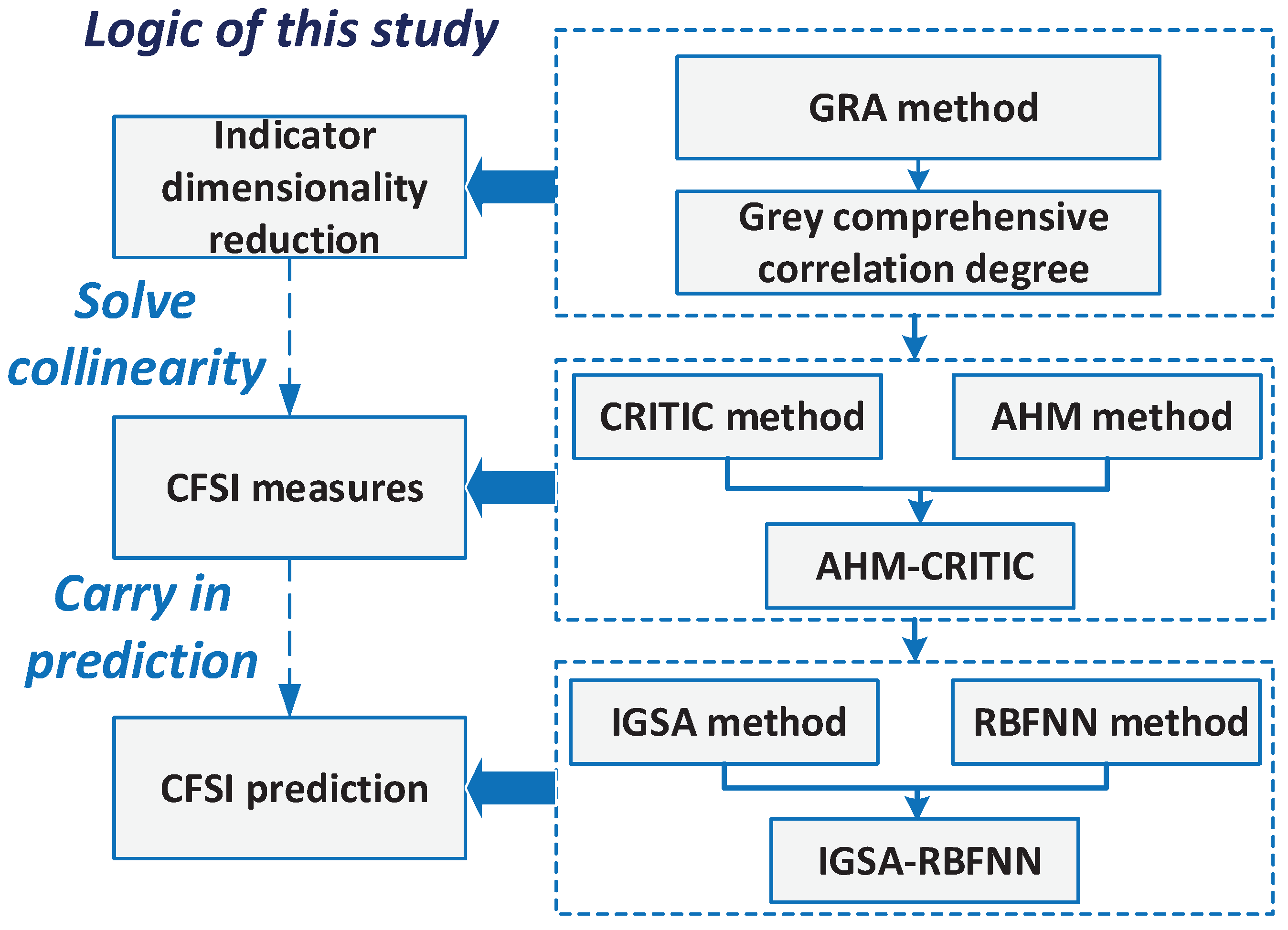
Figure 3.
IGSA-RBFNN structural.
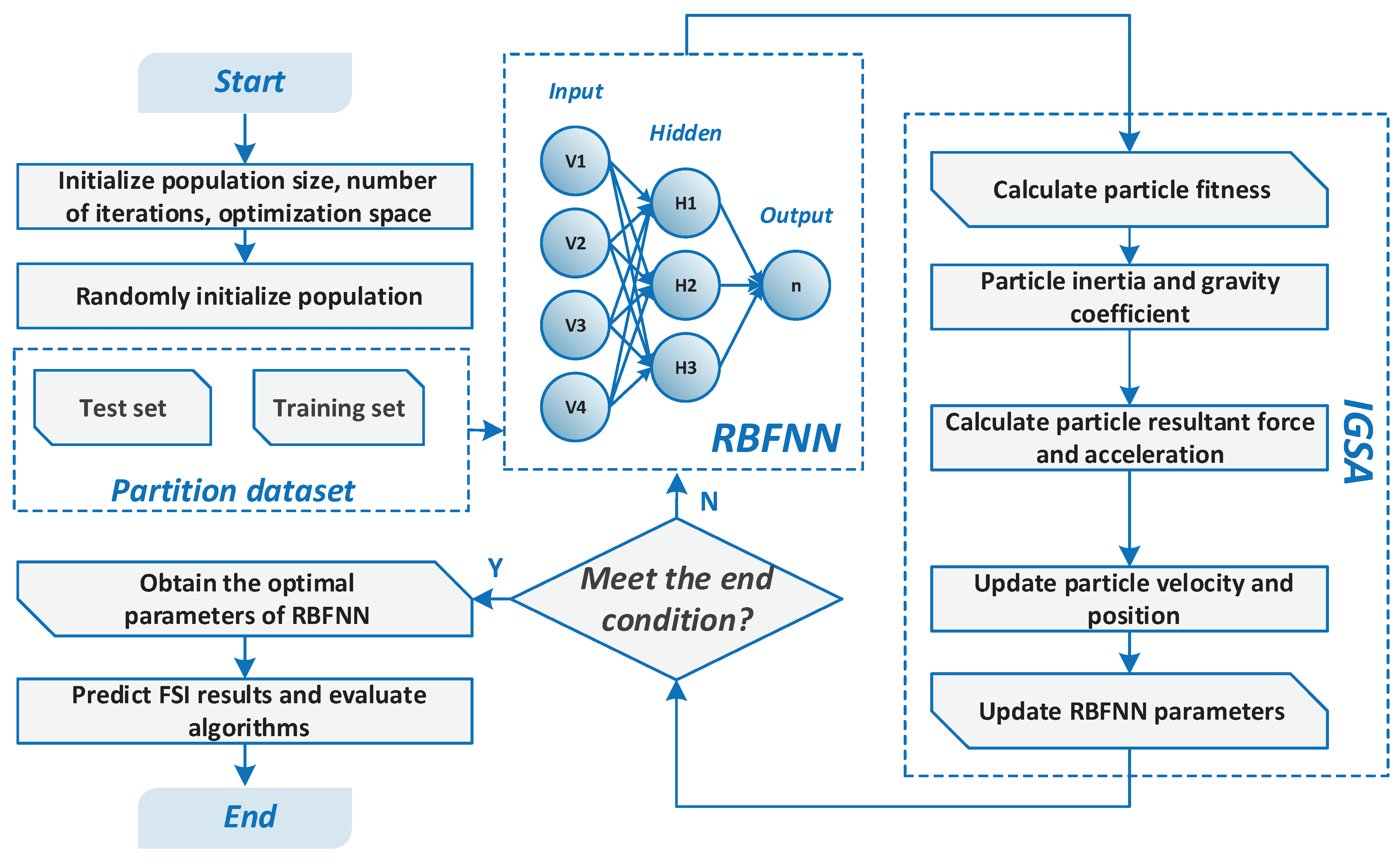
Figure 4.
Correlation matrix of standardized data.
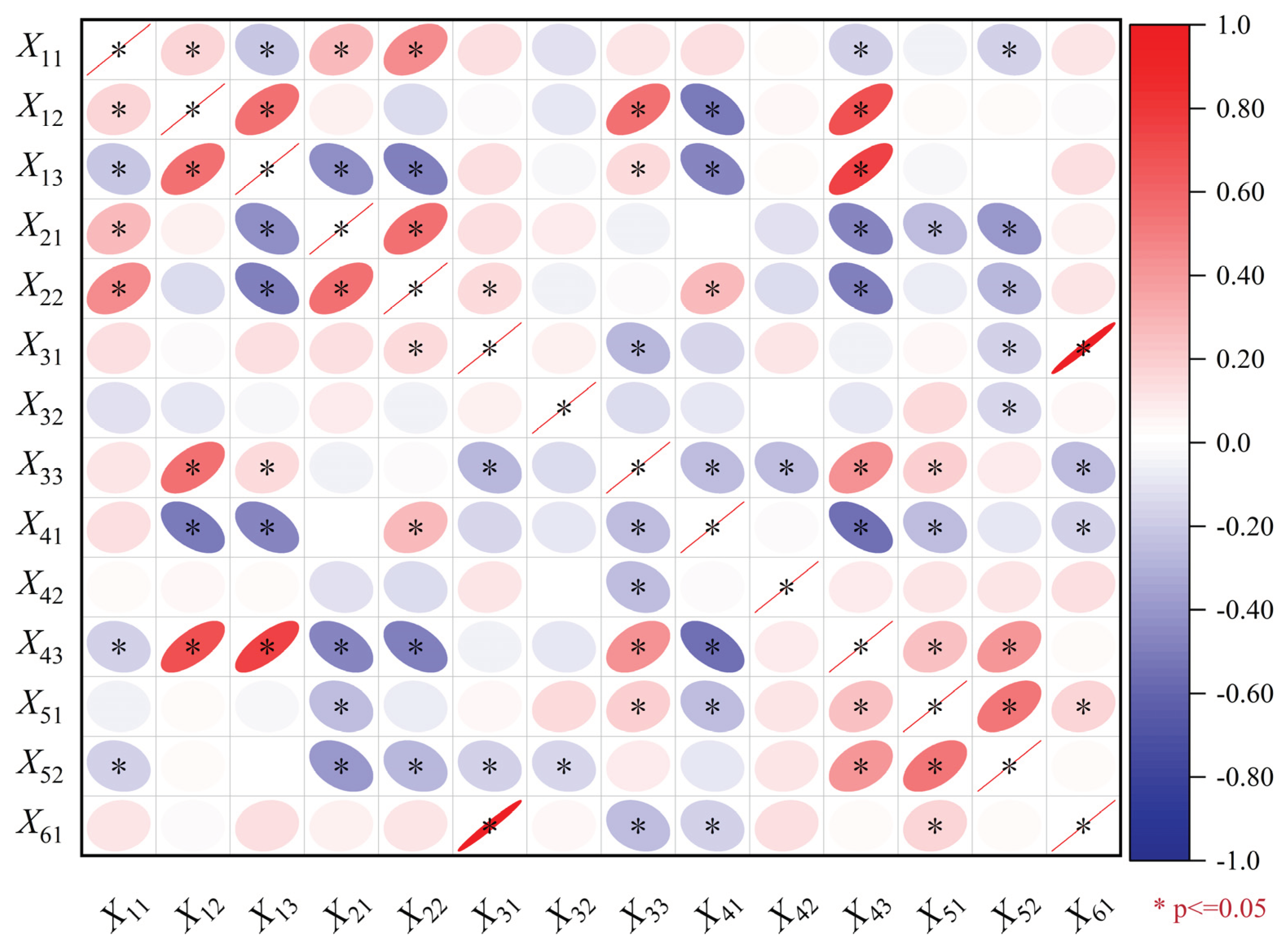
Figure 5.
China financial pressure index measurement results. (a) MFSI Index Chart; (b) BFSI Index Chart; (c) SFSI Index Chart; (d) EFSI Index Chart; (e) TCFSI Index Chart; (f) EDFSI Index Chart; (g) CFSI Index Chart.
Figure 5.
China financial pressure index measurement results. (a) MFSI Index Chart; (b) BFSI Index Chart; (c) SFSI Index Chart; (d) EFSI Index Chart; (e) TCFSI Index Chart; (f) EDFSI Index Chart; (g) CFSI Index Chart.
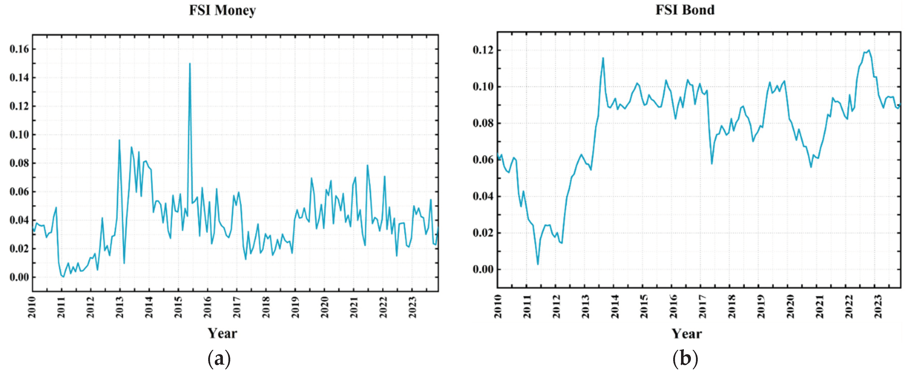
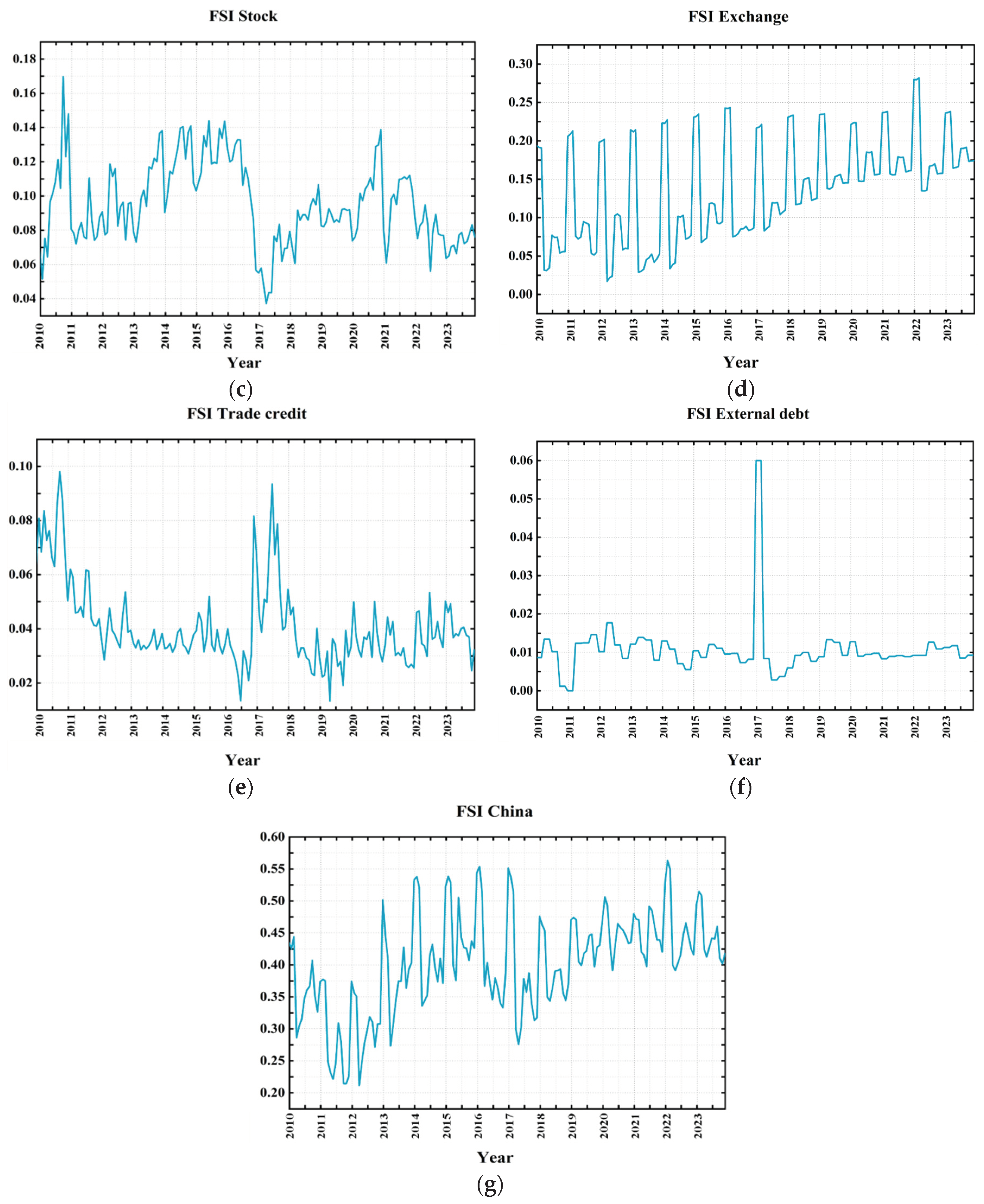
Figure 6.
CFSI prediction results. (a) MFSI Forecast Chart; (b) BFSI Forecast Chart; (c) SFSI Forecast Chart; (d) EFSI Forecast Chart; (e) TCFSI Forecast Chart; (f) EDFSI Forecast Chart; (g) CFSI Forecast Chart.
Figure 6.
CFSI prediction results. (a) MFSI Forecast Chart; (b) BFSI Forecast Chart; (c) SFSI Forecast Chart; (d) EFSI Forecast Chart; (e) TCFSI Forecast Chart; (f) EDFSI Forecast Chart; (g) CFSI Forecast Chart.
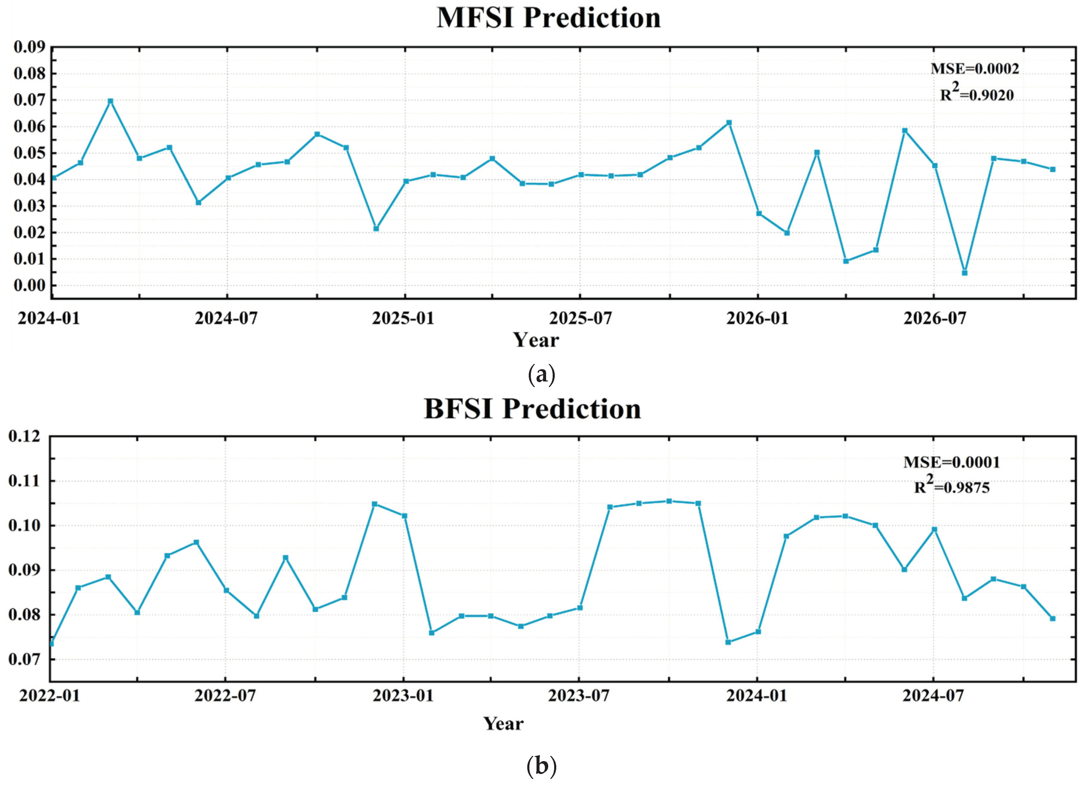
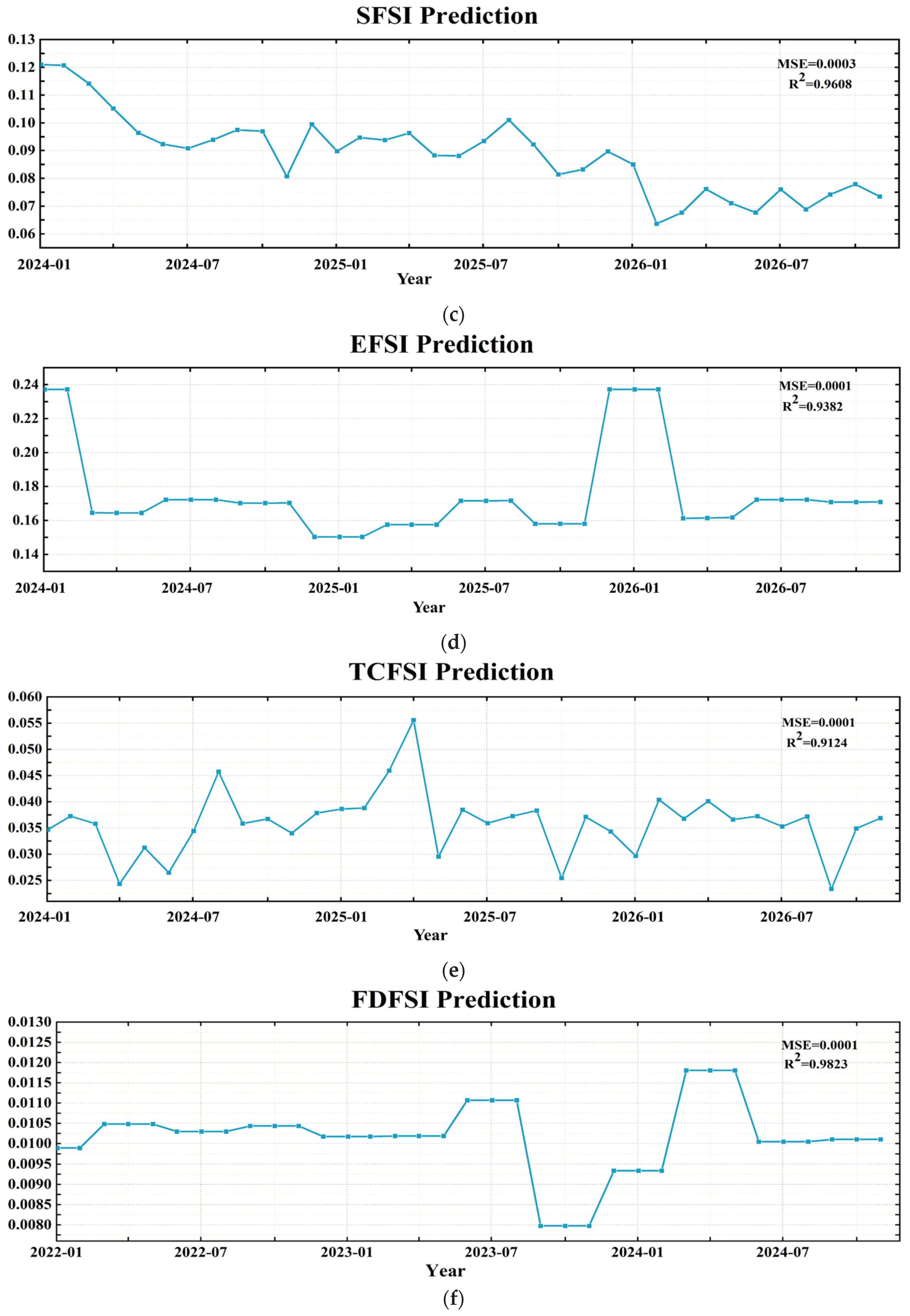
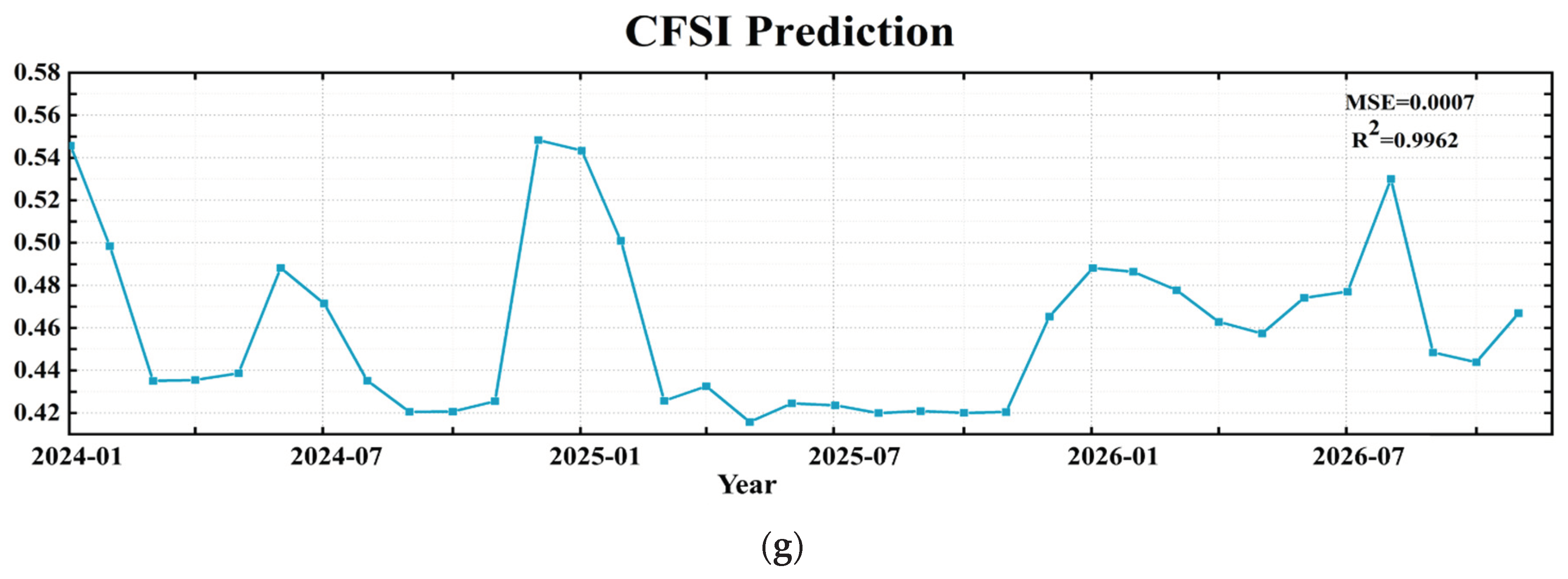
Figure 7.
MSE accuracy comparison.
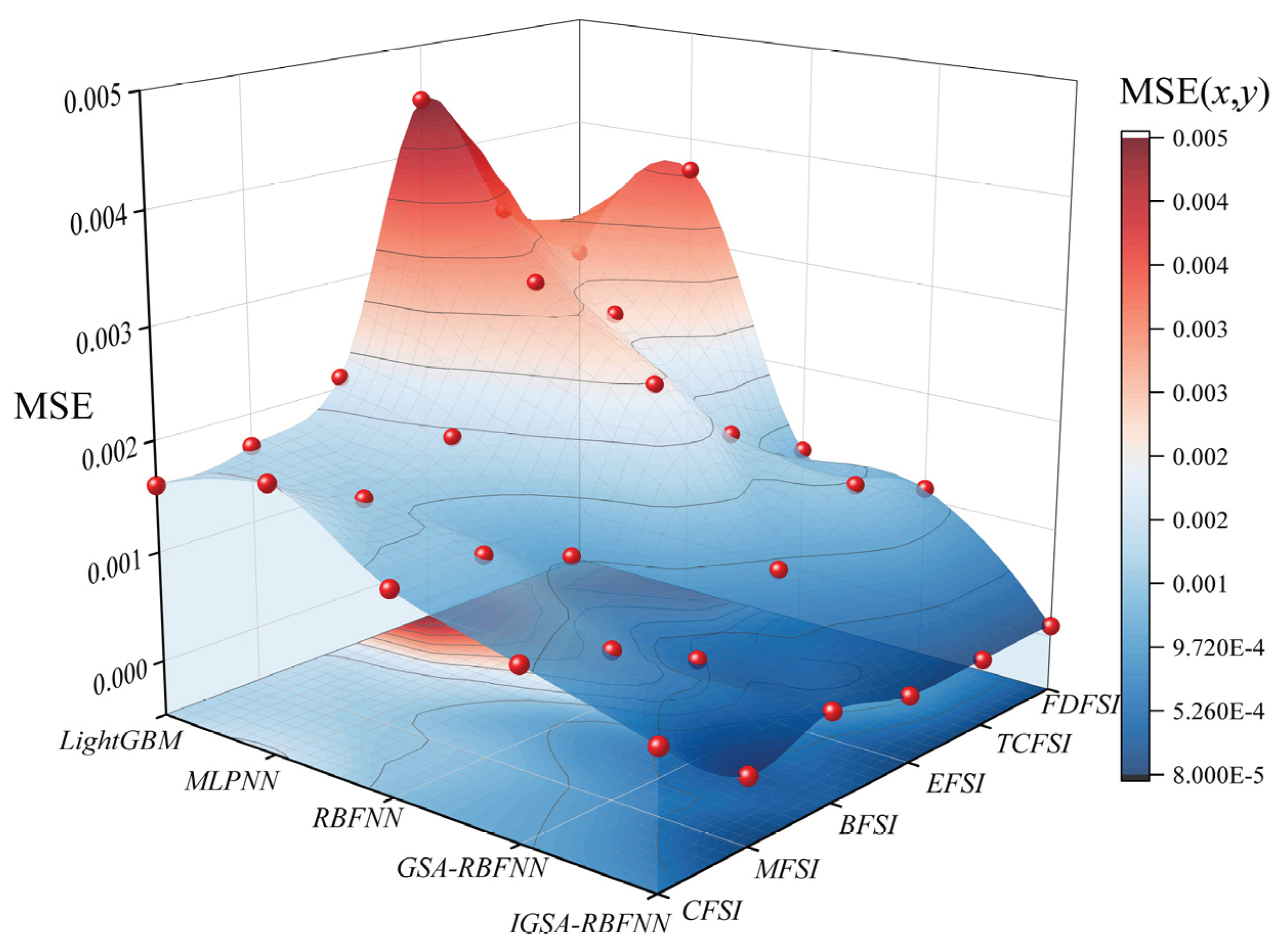
Figure 8.
R2 accuracy comparison.
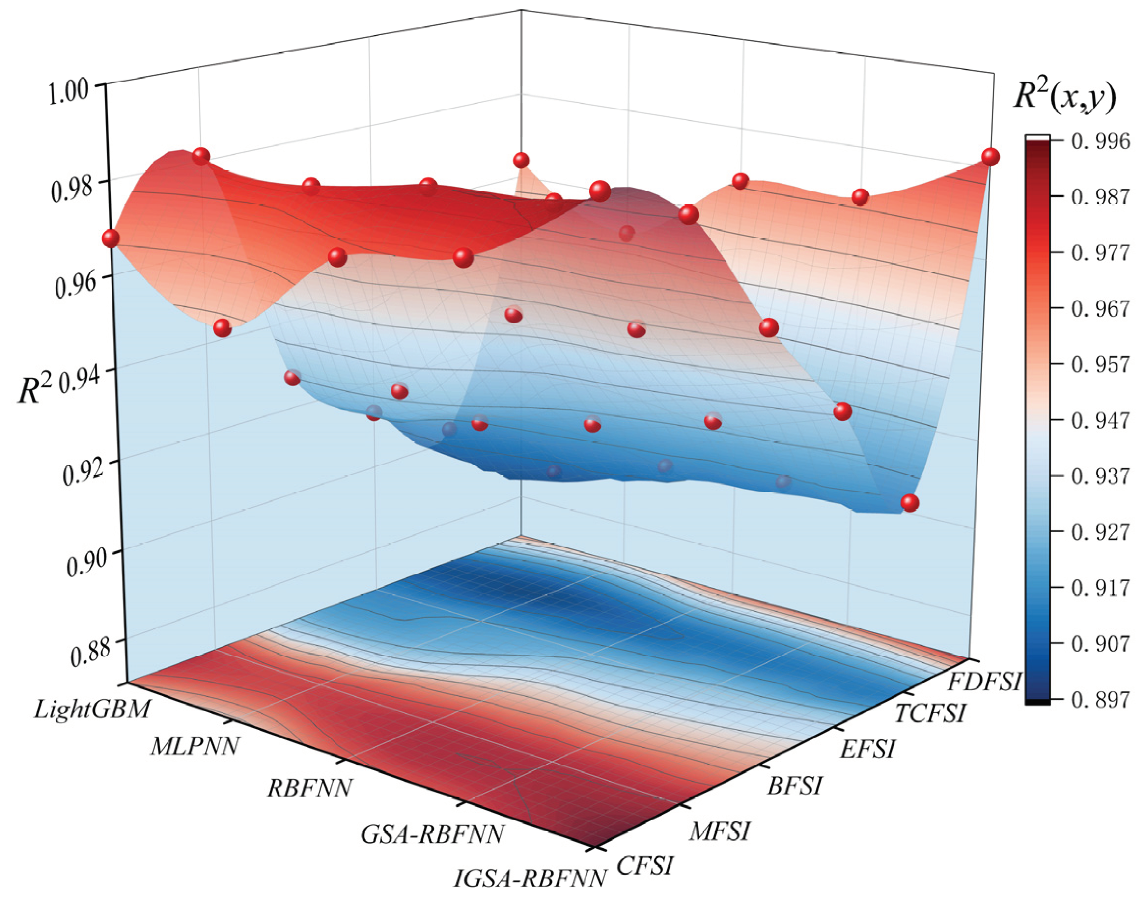
Table 1.
CFSI indicators.
| System layer | Indicators layer | Variable Nature | Unit | Source of indicators/ Periodicity | Reference |
| Money market (X1) | Interbank Spread (X11) | Positive | Million yuan | People's Bank of China / Monthly data | [44] |
| Growth Rate of Short-Term Loans (X12) | Positive | % | People's Bank of China / Monthly data | [16] | |
| SHIBOR(X13) | Positive | % | People's Bank of China / Monthly data | [46] | |
| Bond market (X2) | Sovereign Bond Spreads (X21) | Positive | % | WIND/ Monthly data | [5] |
| Stock market (X3) | Negative Term Bond Spread (X22) | Positive | % | WIND/ Monthly data | [46] |
| CSI 300 Index Yield (X31) | Positive | % | WIND/ Monthly data | [48] | |
| CSI 300 Index Fluctuation Range (X32) | Positive | % | WIND/ Monthly data | [49] | |
| Exchange market (X4) | Stock Market Value/GDP (X33) | Positive | - | WIND/ Quarterly data | [16] |
| Yield of USD to RMB (X41) | Positive | % | Guotaian / Daily data | [24,46] | |
| Changes in foreign exchange reserves (X42) | Positive | % | Guotaian / Quarterly data | [24] | |
| Trade credit market (X5) | Vulnerability of foreign exchange market (X43) | Positive | - | Guotaian / Monthly data | [22] |
| Banking System Beta (X51) | Positive | - | WIND/ Monthly data | [47] | |
| Bank Index Volatility (X52) | Positive | % | WIND/ Monthly data | [47] | |
| External debt market (X6) | Growth Rate of Total External Debt (X61) | Negative | % | WIND/ Quarterly data | [48] |
Table 2.
Descriptive statistics of indicators.
| Indicators | Max | Min | Mid | Mean |
| X11/ million yuan | 49309.00 | 4415.00 | 15479.50 | 16231.43 |
| X12/% | 0.23 | 0.03 | 0.09 | 0.12 |
| X13/% | 6.69 | 0.80 | 2.27 | 2.30 |
| X21/% | 2.43 | -0.62 | 1.23 | 1.09 |
| X22/% | -0.03 | -2.22 | -0.67 | -0.81 |
| X31/% | 0.04 | 0.01 | 0.02 | 0.01 |
| X32/% | 25.81 | -25.85 | 0.44 | 0.26 |
| X33 | 0.05 | 0.02 | 0.03 | 0.03 |
| X41/% | 0.02 | 0.00 | 0.01 | 0.01 |
| X42/% | 0.33 | -0.22 | -0.07 | -0.01 |
| X43 | 0.29 | 0.09 | 0.19 | 0.18 |
| X51 | 1.67 | 0.02 | 0.75 | 0.76 |
| X52/% | 0.05 | 0.01 | 0.01 | 0.02 |
| X61/% | -0.05 | 0.29 | 0.01 | 0.01 |
Table 3.
AHP Discriminant matrix K.
| X1 | X2 | X3 | X4 | X5 | X6 | |
| X1 | 1 | 3 | 1 | 1/3 | 4 | 3 |
| X2 | 1/3 | 1 | 1/2 | 1/4 | 1 | 3 |
| X3 | 1 | 2 | 1 | 1/2 | 3 | 3 |
| X4 | 3 | 4 | 2 | 1 | 5 | 4 |
| X5 | 1/4 | 1 | 1/3 | 1/5 | 1 | 3 |
| X6 | 1/3 | 1/3 | 1/3 | 1/4 | 1/3 | 1 |
Table 4.
AHM attribute discrimination matrix L.
| X1 | X2 | X3 | X4 | X5 | X6 | |
| X1 | 0 | 6/7 | 1/2 | 1/7 | 8/9 | 6/7 |
| X2 | 1/7 | 0 | 1/5 | 1/9 | 1/2 | 6/7 |
| X3 | 1/2 | 4/5 | 0 | 1/5 | 6/7 | 6/7 |
| X4 | 6/7 | 8/9 | 4/5 | 0 | 10/11 | 8/9 |
| X5 | 1/9 | 1/2 | 1/7 | 1/11 | 0 | 6/7 |
| X6 | 1/7 | 1/7 | 1/7 | 1/9 | 1/7 | 0 |
Table 5.
Weighing outcomes and combining the weights of various approaches.
| AHM | CRITIC | |||||||
| 0.19 | 0.11 | 0.02 | 0.21 | 10.63 | 2.18 | 0.09 | 0.04 | |
| 0.31 | 0.06 | 0.15 | 10.81 | 1.63 | 0.06 | 0.06 | ||
| 0.58 | 0.10 | 0.22 | 11.56 | 2.49 | 0.10 | 0.10 | ||
| 0.10 | 0.75 | 0.08 | 0.22 | 9.41 | 2.03 | 0.08 | 0.08 | |
| 0.25 | 0.03 | 0.23 | 8.73 | 1.98 | 0.08 | 0.05 | ||
| 0.20 | 0.75 | 0.15 | 0.16 | 9.17 | 1.51 | 0.06 | 0.10 | |
| 0.25 | 0.05 | 0.14 | 9.04 | 1.24 | 0.05 | 0.05 | ||
| 0.37 | 0.75 | 0.28 | 0.29 | 11.62 | 3.33 | 0.13 | 0.20 | |
| 0.25 | 0.10 | 0.33 | 10.38 | 3.43 | 0.13 | 0.12 | ||
| 0.09 | 0.17 | 0.02 | 0.16 | 11.03 | 1.81 | 0.07 | 0.04 | |
| 0.83 | 0.07 | 0.20 | 13.40 | 2.63 | 0.10 | 0.09 | ||
| 0.06 | 1 | 0.06 | 0.12 | 10.82 | 1.33 | 0.05 | 0.06 | |
Disclaimer/Publisher’s Note: The statements, opinions and data contained in all publications are solely those of the individual author(s) and contributor(s) and not of MDPI and/or the editor(s). MDPI and/or the editor(s) disclaim responsibility for any injury to people or property resulting from any ideas, methods, instructions or products referred to in the content. |
© 2024 by the authors. Licensee MDPI, Basel, Switzerland. This article is an open access article distributed under the terms and conditions of the Creative Commons Attribution (CC BY) license (http://creativecommons.org/licenses/by/4.0/).
Copyright: This open access article is published under a Creative Commons CC BY 4.0 license, which permit the free download, distribution, and reuse, provided that the author and preprint are cited in any reuse.


