Submitted:
18 March 2024
Posted:
19 March 2024
You are already at the latest version
Abstract
This study addresses the critical challenge of Speech Enhancement (SE) in noisy environments, where the deployment of Deep Neural Networksolutions on microcontrollers is hindered by their extensive computational demands. Focusing on this gap, our research introduces a novel SE method optimized for MCUs, employing a 2-layer GRU model that capitalizes on perceptual speech properties and innovative training methodologies. By incorporating self-reference signals and a dual strategy of compression and recovery based on the Mel scale, we develop an efficient model tailored for low-latency applications. Our GRU-2L-128 model demonstrates a significant reduction in size and computational requirements, achieving a 14.2× decrease in model size and a 409.1× reduction in operations compared to traditional DNN methods like DCCRN, without compromising performance. This advancement offers a promising solution for enhancing speech intelligibility in resource-constrained devices, marking a pivotal step in SE research and application.
Keywords:
GRU
; Self-Reference
; speech enhancement
1. Introduction
In audio signal processing, Speech Enhancement (SE) is crucial because environmental noise, from city traffic to the buzz of crowded places, often makes spoken words hard to understand [1]. This is especially true for people with hearing loss. Their importance becomes even more pronounced in applications such as voice recognition systems and telecommunications, where ambient noise can significantly hinder performance and user satisfaction. Hearing aids, vital tools for millions, have come a long way, with modern devices leveraging intricate algorithms to optimize the listening experience. These algorithms, which encompass directional processing [2,3], automatic gain control [4,5,6], and single-channel noise reduction [7,8], are purpose-built to enhance the signal-to-noise ratio (SNR) in various conditions. However, while techniques like directional processing show promise, especially in non-stationary noise scenarios they aren’t without their limitations.
Despite these advances, there remain significant challenges in the realm of SE. Classical algorithms that rely heavily on first and second-order statistics [9], for instance, often falter in scenarios with non-stationary noises [10,11]. Their performance, in many cases, leaves much to be desired. The conundrum deepens when we consider that many existing algorithms, while adept at minimizing white noises, struggle against the unpredictability of non-stationary noises. Previous studies have attempted to navigate these challenges, with solutions such as the codebook-based NR [12]. However, the robustness of such solutions, especially when applied to critical medical devices like hearing aids, remains a topic of debate. A significant stride in recent years has been the advent of deep neural network (DNN) based noise reduction. Within the time-frequency domain, the trajectory of neural network architectures has evolved from the early use of recurring neural networks, notably the RNNoise [13] model, to advanced encoder-decoder frameworks like the DCCRN [14] and DCUNet [15]. Recent innovations have introduced transformer-based models such as DPTNet [16], enhancing context-aware modeling, alongside breakthroughs in noise suppression with NSNet [17] and NSNet2 [18]. These DNN solutions have showcased a marked improvement over their traditional counterparts, particularly in environments dominated by low-SNR non-stationary noises.
The shift to DNN-based speech enhancement represents a leap forward but exposes a critical research gap: the dominance of large-parameter models unsuited for MCUs like the STM32 series, where efficiency and power are key as shown in Table 1. Despite TinyLSTM [19] pivotal contributions in model compression for speech enhancement, a significant gap remains in exploring the training methodologies for such resource-limited models. Current research, including TinyLSTM predominantly focuses on post-training compression techniques like pruning and quantization.
Building on the foundation laid by NSNet [17,18], this study shifts focus towards innovating training methodologies for RNN-based speech enhancement models suited for MCUs. Our research investigates training methodologies, aiming to optimize model performance from the start rather than adjusting post-training. In this work, we present an SE method based on 2-layers GRU aimed for low-latency requirements. We exploit perceptual properties of speech for designing an efficient end-to-end model. Our approach introduces self-reference signals to mitigate the uncertainties in SE tasks, effectively compensating for performance degradation due to model downsizing. We counteract the performance dip from downsizing the model by squaring the magnitude spectrum to concentrate speech energy. By contrasting this with the original signal, we simplify training and enhance model effectiveness. We also tackle audio signal compression to 128 hidden layers and its required expansion back to 256. Using compression and recovery techniques with trainable parameters based on the Mel scale, we enhance performance. This dual strategy of utilizing self-reference signals and advanced compression methods enables our GRU-2L-128 model to achieve optimal performance with limited computational resources. We find that we can match the performance of DCCRN methods with a reduction in model size and operations of 14.2× and 409.1×.
2. Background
2.1. Deep Learning Based Speech Enhancement
SE technologies have evolved significantly, branching into two primary domains: the time domain and the time frequency domain (T-F).
Time Domain
In the time domain, speech enhancement methods typically involve direct mapping of noisy one-dimensional waveforms to clean 1D waveforms [20,21]. This approach has been popularized through the use of encoder-decoder or UNet structures [21], where the encoder translates noisy speech into a feature domain, and the decoder reconstructs enhanced features back into the time domain. Inserted between the encoder and decoder is the enhancement module, often utilizing long-short term memory or temporal convolutional networks to leverage temporal correlations. Despite the effectiveness of time domain methods in speech enhancement, it has been observed that noise patterns are more distinguishable in the T-F domain.
Time-Frequency Domain
In contrast, T-F domain methods focus on predicting a mask to model the relationship between targeted and noisy speech. Initially, methods such as the ideal binary mask [22] and ideal ratio mask [23] (IRM) were employed, modeling only the magnitude relationship and inadvertently neglecting phase information. This omission limited the enhancement potential of these methods.
In the evolution of neural network architectures for time-frequency domain speech enhancement, the field has transitioned from the early utilization of Recurrent Neural Networks (RNNs), exemplified by the foundational RNNoise [13] model, to more sophisticated encoder-decoder structures such as the Deep Complex Convolution Recurrent Network [14] (DCCRN) and the Deep Complex U-Net [15] (DCUnet). This progression continued with the advent of transformer-based models like the Dual-Path Transformer Network (DPTNet) [16], which represented a significant leap in context-aware modeling. Moreover, developments in noise suppression techniques, particularly NSNet [17] and NSNet2 [18], introduced innovative learning objectives that enhanced speech quality. Each stage in this continuum of architectural evolution has not only demonstrated an increase in complexity and sophistication but has also significantly contributed to the advancement of speech processing technologies, illustrating a steadfast commitment to improving speech enhancement methodologies.
2.2. Reference-Based Approach
Reference-based approaches, deriving inspiration from image restoration, have risen in prominence, offering innovative solutions to traditional problems. Such methods leverage high-quality references to aid in the restoration of degraded signals, emphasizing the importance of patch-level similarities between the reference and degraded signals.
In the domain of image processing, reference-based image restoration has demonstrated its efficacy in works, such as RefSR [24,25,26] and Ref-denoising [27]. Traditional methodologies employed by Yue et al [24,27]. emphasized searching for analogous patches in the pixel domain within high-quality reference images. These similar patches were then harnessed to assist in the restoration of the degraded counterpart. With the proliferation of deep learning techniques [25,26,28], there was a perceptible shift in patch search methodologies. Instead of the pixel domain, contemporary methods began searching for analogous patches in the CNN feature domain. Notably, these CNN-based methodologies allow the setting of feature extraction networks in well-established architectures such as VGG or ResNet.
There is a method [29] to improve speech quality by extracting Mel frequency spectral coefficients (MFCCs) from noisy signals and improving them using deep features from high-quality reference MFCCs spectrograms.
2.3. QDNN
Quadratic Deep Neural Networks (QDNNs) represent a shift in DNN technology. Moving away from the conventional DNN approach that uses a linear combination of input variables, QDNNs employ a second-order polynomial to represent neurons. This offers several distinct advantages: Firstly, they exhibit enhanced nonlinearity, leading to a superior capacity for feature extraction [33]. Secondly, QDNNs are known for their model efficiency [31]. Due to their structure, they can approximate polynomial decision boundaries even with more concise network configurations. Third, in the realm of Privacy-Preserving Machine Learning [39,40,41], QDNNs bring about computational savings, particularly when ReLU is replaced with a quadratic layer. Examining the nuances of QDNN designs, there are four main types as shown in Table 2: T1 has inputs that interact through an outproduct with a full-rank weight matrix [30,31,32,33,34]; T2 achieves the second order term by directly squaring each input [35]; T3 sources its second-order term from the square of a first order primary neuron [36]; and T4 computes the second-order term using the Hadamard product of two distinct first order neurons, each with its own set of weight parameters [37].
However, despite these advantages, there are notable challenges associated with QDNNs. Some designs, like T2 and T3, grapple with approximation capability issues due to a lack of trainable parameters. This deficiency could hinder their theoretical performance. The T1 design, on the other hand, introduces computational complexity challenges. Its inclusion of a full-rank weight matrix in each neuron can lead to potential memory issues during training, especially as the model’s depth and width expand. Furthermore, several QDNN designs, including those cited in studies like Cheung Leung et al. [30], demand more intermediate parameters during the training process. These parameters, which must be cached in memory during training, can drain memory resources and lead to inefficiencies.
3. Methods
3.1. Signal Model
Let x(t) be a mixture signal
where s(t) is a clean speech signal and z(t) is an interfering backgroud noise. Typically HA noise reduction opearte in STFT domain:
where , , and symbolize the STFT at time frame t and frequency bin f for the observed noisy speech, the underlying clean speech, and the noise component, respectively. The central aim of our system is to devise a time-variant gain function in the STFT magnitude (STFTM) domain, denoted by , which is optimized to approximate the magnitude of the clean speech signal as accurately as possible. This objective is encapsulated in the equation:
In scenarios necessitating real-time processing, the function is formulated to depend exclusively on the past and current inputs. This dependency is represented as follows:
where f signifies a transformation function applied to the STFTM of the noisy signal, and n denotes a DNN characterized by its adjustable parameters collectively referred to as . The final step in obtaining the enhanced signal involves the application of the noisy phase of to .
3.2. Self-Reference Based Approach
To adapt to the limitations of edge devices and achieve real-time streaming inference, the computational load of the model needs to be controlled within 50 MMACs/s. Therefore, GRU-2L-128 was chosen as the base model structure. However, it was found in actual training that the performance of directly trained GRU-2L-128 significantly declined compared to larger models like GRU-2L-256 or GRU-2L-512. To overcome the performance degradation issue of lightweight models, this paper proposes introducing self-referential signals, aiming to enhance model performance or avoid performance degradation by providing more prior information.
Speech signals show significant sparsity in their temporal distribution, meaning their energy is concentrated, and in low signal-to-noise ratio environments, the elimination of stationary noise is relatively more challenging. To emphasize the sparsity in the input features, thereby reducing the learning difficulty for small models, a simple method is to apply a monotonically increasing function to strengthen the input features, such as , where essentially emphasizes the power spectrum. Through this transformation, the energy distribution of the noisy spectrogram becomes more prominent, thus helping the model better distinguish between speech signals and noise.
However, if only the transformed features are used as model inputs, it may still confuse the model, as the model essentially predicts the mask on the original signal. To address this issue, the method proposed in this chapter is to provide both the original amplitude spectrum and derived signals (such as the power spectrum) as input features to the model, allowing the model to utilize both types of information during training. This method allows the model to balance the information from the original amplitude spectrum and the enhanced power spectrum during learning, thus more effectively recovering clean speech signals from noisy signals. Through this self-referential signal strategy, even in lightweight models with limited computing resources, effective enhancement of speech signals in low SNR environments, improving speech clarity and intelligibility, can be achieved.
To fully utilize the sparsity characteristics of speech signals to improve the performance of lightweight models on edge devices, this chapter proposes two self-referential signal features, Noisy2 and Noise as show in Figure 2, aimed at enhancing the model’s ability to distinguish between speech and noise.
1. Noisy2: This feature is obtained by directly squaring the amplitude spectrum of noisy audio, representing the short-term power spectrum of the audio signal. This operation physically amplifies areas with higher energy while compressing areas with lower energy, thus enhancing the contrast between sparse signals (such as speech) and nonsparse signals (such as background noise). In this way, the model can more easily identify and extract key information from speech signals, especially in environments with high noise levels.
2. Noise: Based on the emphasis on signal sparsity with Noisy2, one can further separate the weaker parts from Noisy2 through a projection operator, compared to the original noisy signal (Noisy).
The definition of projection operation is:
which means the corrected target, and the non-target is .
The assumption here is that the relatively weakened components in Noisy2 mainly contain nonsparse noise components. Thus, this feature provides a reference on the noise components, helping the model better distinguish between speech and noise, especially important in handling stationary noise.
In practice, the model receives the original noisy signal (Noisy) and a reference signal (Noise or Noisy2) as inputs and predicts the amplitude spectrum mask to be applied to Noisy based on this information. The effects of the two reference signals are shown in Figure 1.
It is worth noting that the reference signal is obtained through a deterministic calculation process of the input signal x. Theoretically, this process does not introduce additional information, as it is entirely derived from the original signal. However, there are two aspects that make the reference signal potentially valuable for model training in practice:
- The limitations of training data: In training scenarios, since the available speech signals are limited and enumerable, the training data used (e.g., 500 hours of speech signals) is hard to cover all possible speech distributions comprehensively. Therefore, the reference signal can introduce an additional amount of information to some extent, helping the model better understand and utilize the characteristics of speech signals contained in the limited training data.
- The limitations of model capacity: For smaller models, it might be challenging to learn complex features directly from the original signal that are beneficial for the prediction task. In such cases, providing these specifically calculated features as additional input conditions to the model can help the model more effectively capture and utilize key information of speech signals, thereby improving the accuracy and efficiency of predictions.
3.3. Band Compression
Considering the computational and storage limitations of edge devices, compressing the frequency dimension of audio signals has become a necessary step to adapt to the input requirements of the model and maintain real-time processing capabilities. To achieve this goal, this paper introduces a frequency band compression module and a feature expansion module, which are located at the input and output ends of the model, respectively, to adapt to the compressed and expanded frequency band features. This new model architecture allows the model to process more compact frequency representations while ensuring that the final output mask can cover the original frequency range to recover high-quality speech signals.
To explore the most effective frequency band compression strategy, this paper examines four different schemes in detail, each attempting to find the optimal balance between reducing computation and maintaining important signal information:
Linear: This scheme employs a simple linear filter to compress the frequency band at equal intervals, being the most straightforward method of frequency band compression. Although the operation is simple, linear compression may not fully consider the non-linear characteristics of human ear sensitivity to different frequencies, thereby losing important information in speech signals for human hearing to some extent.
Bark: This scheme designs a filter bank based on the Bark scale, better simulating the perceptual characteristics of the human ear towards frequencies. By mimicking the response characteristics of the human auditory system, the Bark filter bank aims to more effectively preserve the frequency components that are more important for human speech recognition, thereby improving the performance of speech enhancement tasks.
Mel: The Mel filter bank is based on the Mel scale, which is designed according to the actual perception of the human ear to different frequencies, emphasizing the components in the speech signal that are more critical to human hearing. The Mel scheme, through non-linear compression of the frequency band, can preserve more speech information during the compression process, especially in the low-frequency area, which is particularly important for speech enhancement tasks.
Mel-Learn (Learnable Mel): Unlike traditional Mel filter banks, the Mel-Learn scheme allows filter parameters to be learned and adjusted during the training process. This design enables the model to adaptively optimize the frequency band compression strategy to suit specific task needs. By allowing the model to learn the most suitable frequency band compression method on its own, it is hoped to further improve the speech enhancement effect.
3.4. Learning Machine and Loss Function
In our methodological framework, we develop a machine learning model tailored for speech enhancement. This model operates by inputting a single frame of noisy speech and producing the corresponding frame of the gain function. At the core of our system is the Gated Recurrent Unit (GRU). We preferred GRUs over Long Short-Term Memory units due to their computational efficiency and demonstrated efficacy in real-time speech enhancement tasks.
Our model’s architecture involves a sequential arrangement of two GRU layers, each of which refines the understanding gleaned from the previous one. Following these GRU layers, we incorporated a fully connected output layer with a sigmoid activation function, ensuring that the output, the gain function G[t, k], remains within a normalized range.
We employ the projected loss function introduced in our recent work [42]:
which, represents the use of the Voice Activity Detection (VAD) algorithm to filter out the inactive parts of the audio.
The loss function is divided into two parts: the first part requires the model to fit the gain function G to the target audio; the second part demands that the model’s gain function, when inverted, fits the non-target parts as closely as possible. These two learning objectives describe the same concept but their combined use ensures the model remains stable during training without deviating too far from the target outcome.
The proposed method is illustrated in a flowchart in Figure 2. To compute the loss during training, both clean and noisy speech samples are needed. The trained model processes the noisy STFT Magnitude frame by frame and uses the noisy phase information to reconstruct the enhanced speech waveform. To avoid high computation complexity, the model receive the mixing signal which contacting orginal signal and reference signal.
4. Experiment
4.1. Datasets
In our research, we mainly use DNS 2021 [43] for the training of our model. Data are meticulously segmented according to signal intensity, adhering to a distribution 80% / 10% / 10% for training, development and testing phases, respectively. To increase data diversity and counteract overfitting, each training and verification cycle involves the random selection of a voice segment from the training set. This is then paired with a noise segment of equivalent duration, and a random SNR, varying between dB and 15 dB, is applied to dynamically synthesize the noisy speech. For the testing phase, each clean speech segment is juxtaposed with a randomly chosen noise segment, and the synthesis is performed at random SNRs of .
To evaluate the performance of our model, we use the MUSAN [44] and VCTK [45] data sets, which span SNR levels from to . We have curated three test sets for this purpose:
MUSAN Test Set: Encompassing a vast 60 hours of clear speech and an additional 48 hours of music and environmental noise, this set evaluates the model’s noise reduction capabilities. We utilize all clean speech, treating the combined 48 hours as noise data.
Babble Test Set [46]: Derived from the Babble noise dataset and MUSAN’s clean speech, this set tests the model’s ability to handle interference, especially since Babble noise shares energy distribution characteristics with speech signals.
VCTK Test Set: A combination of VCTK’s clean speech and the stationary noises from NoiseX92, this set assesses the model’s skill in eliminating persistent noise.
The NoiseX92 dataset [47] offers a collection of stationary noises from real-world settings such as factories, engine rooms, and vehicles. In contrast, the Babble dataset from MyNoise replicates the bustling environment of a cafe, with its chaotic chatter and distinct cafe sounds, challenging the model due to its noise components’ resemblance to speech signals.
Lastly, All test sets maintain a uniform SNR distribution.
4.2. Evaluation Metrics
PESQ [48,49]: Perceptual Evaluation of Speech Quality is a standardized objective measurement algorithm employed for evaluating the quality of speech transmission within telecommunications networks. Assesses perceived speech quality by comparing original and degraded speech signals, assigning a score that reflects the degree of similarity between the degraded and original signals. Scores are typically represented on a -0.5 to 4.5 scale, where higher values denote superior quality.
STOI [50]: Short-Time Objective Intelligibility is an established metric for assessing the intelligibility of speech signals by quantifying the extent to which a degraded or distorted speech signal can be comprehended in comparison to a reference clean speech signal. The STOI algorithm conducts a comprehensive analysis of the spectral and temporal characteristics inherent in the speech signals, producing a similarity score that ranges from 0 to 1, where 0 denotes no intelligibility and 1 represents perfect intelligibility.
4.3. Baseline and Compared Model
To assess the objective performance of HA, our approach is compared with the following baselines using the DNS test corpus.
FullSubNet+ [51]: an enhanced single-channel real-time speech enhancement framework. The FullSubNet+ model incorporates multiscale time-sensitive channel attention and utilizes complex spectrograms as input to improve noise reduction in audio signals.
DCCRN [14]: Deep Complex Convolution Recurrent Network simulates complex-valued operations for speech enhancement. The DCCRN model combines the strengths of convolutional encoder-decoder structures with LSTM to effectively handle complex-valued operations in the time-frequency domain.
DPTNet [16] : Dual-path transformer network emphasizes direct context-aware modeling for speech sequences, allowing for direct interactions between elements in speech sequences. The improved transformer integrates a recurrent neural network to learn sequence order without positional encodings.
DCUnet [15] : Deep Complex U-Net, a model tailored for speech enhancement that addresses the challenge of phase estimation. The authors propose a method to handle complex-valued spectrograms using a polar coordinate-wise complex-valued masking approach. Additionally, they introduce a novel loss function, the weighted source-to-distortion ratio (wSDR) loss, to improve the model’s effectiveness.
DPRNN [52]: dual-path recurrent neural network for efficient modeling of long sequences in time-domain speech separation. The DPRNN method divides the input into smaller chunks and uses intra- and inter-chunk operations for processing. This approach addresses the challenges faced by traditional RNNs and 1-D CNNs in handling long sequences.
RNNoise [13]: hybrid approach combining DSP techniques and deep learning for real-time speech enhancement with low computational complexity.
NSNet [17]: proposing two novel learning objectives that allow for separate control over speech distortion and noise reduction and examining the effects of feature normalization and sequence lengths on speech quality.
NSNet2 [18]:s a scalable speech enhancement method using a convolutional recurrent network that significantly improves speech quality with low computational cost.
The Table 3 compares speech enhancement models, showing that models like FullSubNet+, and others have high computational complexity, indicated by their large number of parameters and high processing speeds. These models are designed for environments with significant computational resources, such as desktops, highlighting their ability to handle complex audio processing tasks efficiently. On the other hand, RNN-Noise and NSNet stand out for their low computational requirements. RNN-Noise, with only 0.87M parameters and a processing speed of 0.04 GMACs/s, and NSNet, with 1.32M parameters and a processing speed of 0.17 GMACs/s, are optimized for environments with limited computational power. This makes them suitable for applications in edge streaming and ARM streaming, respectively, where conserving computational resources is crucial.
5. Results
5.1. Compare Performance with Other Models
In this study, as shown in Table 4, we evaluated the GRU-2L-128 model on the DNS test set for speech enhancement. This model significantly outperforms the original noisy audio recordings in terms of PESQ and STOI metrics, with improvements from 1.710 to 2.175 for PESQ and from 0.713 to 0.768 for STOI. Compared to state-of-the-art models like DCCRN and DCUNET, GRU-2L-128 shows remarkable performance, especially in low SNR conditions where it outperforms DCCRN by improving from 1.544 to 1.729 in PESQ and exhibits a slight advantage over DCUNET with an improvement to 1.729 in PESQ. Despite a small gap with DCUNET in high SNR conditions, GRU-2L-128 maintains competitive performance. Against models with similar structures, such as Nsnet2, GRU-2L-128 achieves slightly better results in low SNR scenarios with less computational cost and parameters, improving PESQ from 1.702 to 1.729. Compared to GRU-2L-256, GRU-2L-128 shows a slight decrease in PESQ but maintains similar performance in high SNR ranges. Overall, GRU-2L-128 significantly surpasses the RNN-Noise model in all metrics, especially in low SNR conditions where PESQ improved from 1.439 to 1.729 and STOI from 0.579 to 0.668. In high SNR scenarios, PESQ and STOI also saw substantial increases. These results demonstrate GRU-2L-128’s superior speech enhancement performance in various noise environments and low SNR conditions.
In the performance comparison on the Speech Babble test set, as shown in Table 5, models like DPTNET, DPRNN, DCUNET, and DCCRN saw significant performance declines and are not compared here. The GRU-2L-128-learn model improved in high SNR scenarios, with PESQ increasing from 2.106 to 2.356 and STOI from 0.883 to 0.889, indicating optimized speech quality. However, performance slightly decreased in low SNR ranges, with a drop in PESQ from 1.486 to 1.429 and a minor decrease in STOI. Compared to the Rnn Noise model, GRU-2L-128-learn had a slightly higher STOI in low SNR scenarios (0.515 vs. 0.504), suggesting about a 1% improvement in intelligibility. Against Nsnet2, GRU-2L-128-learn was slightly lower in both STOI (0.675 vs. 0.684) and PESQ (1.826 vs. 1.898), showing comparable clarity but about 1% lower intelligibility.The GRU-2L-128 model showed some disadvantages compared to Rnn-Noise in high SNR conditions on the Speech Babble set. This could be due to training data differences, where Rnn-Noise’s inclusion of crowd noise may have enhanced its performance, and the loss of frequency band information, as noise reduction in Speech Babble requires reliance on non-primary energy regions. The GRU-2L-128’s compression of audio bands to 64 might lead to information loss in these areas. The performance comparison on the VCTK test set demonstrates the effectiveness of the GRU-2L-128 model as shown in Table 6. When compared to the noisy audio baseline, the model enhances the overall PESQ from 1.774 to 2.189 and improves the overall STOI from 0.683 to 0.709. In low SNR conditions, the GRU-2L-128 notably outperforms the current DCCRN, raising the PESQ from 1.692 to 1.770 and the STOI from 0.567 to 0.610. Despite its similar structure to Nsnet2, GRU-2L-128 shows slightly lower metrics, with a total PESQ of 2.189 compared to Nsnet2’s 2.321, and a STOI of 0.709 versus Nsnet2’s 0.726. However, against Rnn-Noise, it exhibits significant improvements in low SNR areas, increasing the PESQ from 1.547 to 1.770 and the STOI from 0.575 to 0.610. Versus the GRU-2L-256 model, GRU-2L-128 not only benefits from reduced computational demands but also demonstrates superior performance, with both overall PESQ and STOI metrics surpassing those of GRU-2L-256.
The experimental results in this subsection demonstrate the powerful performance of the GRU-2L-128 model proposed in this chapter in handling diverse noise environments and steady noise conditions. The model not only shows superior performance compared to other open-source models with similar computational power and architecture but also exhibits competitive strength against advanced models with computational costs up to 300 times higher, such as DCCRN and DCUNET. In crowd noise-dominated Speech Babble scenarios, the GRU-2L-128 model demonstrates good enhancement performance in low SNR ranges. These outcomes highlight the potential and practicality of the self-referencing signal scheme in ultra-lightweight speech enhancement, offering a viable solution for deploying high-performance speech enhancement models at the edge.
5.2. Effect of Reference Signal
This subsection’s experiment aims to explore the impact of different model input features on model performance. In the practice of audio signal processing, taking the logarithm of the square of the input amplitude spectrum is a common processing method. This method can, to some extent, simulate the human ear’s perception of sound intensity and help improve the model’s ability to process speech signals. To thoroughly ablate the impact of input features on model performance, this subsection starts with the logarithmic power spectrum as the benchmark for input features and conducts a series of extended ablation experiments to discuss the specific impact of different types of input features on model performance. For the ablation experiments, the following notations were designed:
1. Nolog: indicates not taking the Log of the input signal.
2. Log: indicates taking the Log of the input signal.
3. Noisy: indicates the amplitude spectrum of noisy audio.
4. Noisy2: represents the square of the amplitude spectrum of noisy audio; this signal is input into the model together with Noisy as a reference signal.
5. Noise: represents the complement of the power spectrum on the original amplitude spectrum; this signal is input into the model together with Noisy as a reference signal.
In this experiment, all frequency band compression methods used a learnable matrix initialized with Mel filter bank parameters. For single-input signals, the signal is compressed to 128 dimensions; for dual-input signals, the two signals are separately compressed to 64 dimensions each and then concatenated before being input into the model. This design aims to explore the comprehensive impact of different input feature combinations on model performance and how optimizing input features can further enhance the model’s performance on speech enhancement tasks.
Experiments on the DNS test set, as shown in Table 7, led to important observations about the impact of input feature types on model performance. The approach without logarithmic transformation, No Log-Noisy2, did not improve over the noisy audio baseline, underscoring the importance of logarithmic transformation for effective training. Applying logarithmic transformation (Log-Noisy2) significantly enhanced model performance, with PESQ and STOI scores increasing to 2.092 and 0.765, respectively, proving its effectiveness. Using original input features (Log-Noisy) slightly decreased performance, indicating reduced noise discrimination capabilities with the original magnitude spectrum. The Log-Noisy2_Noisy method, using Noisy2 as a reference signal, achieved better results, particularly in PESQ and STOI scores, which rose to 2.175 and 0.768, respectively. This shows improved clarity and intelligibility. The Log-Noise_Noisy strategy, which uses Noise as a reference, showed lower performance in terms of clarity and intelligibility compared to the Log-Noisy2_Noisy approach. This indicates that Noise as a reference signal is less effective in varied noise situations.
In the Speech Babble test set experiments evaluating input feature types’ impact on model performance as shown in Table 8, several insights were gathered. The Nolog-Noisy2 approach without logarithmic transformation showed poor performance, with a decrease in PESQ to 1.608 and a significant drop in STOI to 0.490, emphasizing the necessity of logarithmic transformation. Using Log-Noisy2 as input, the model showed balanced improvements, with PESQ increasing to 1.832 and a slight STOI enhancement to 0.688, demonstrating the effectiveness of logarithmic power spectrum features. With Log-Noisy inputs, the model saw a minor PESQ improvement to 1.793 but a STOI decrease to 0.649, indicating a performance decline compared to Log-Noisy2. Utilizing Noise as a reference, the Log-Noise_Noisy model achieved the highest PESQ of 1.860 and an STOI of 0.680, showcasing the advantage of reference signal approaches in noisy voice scenarios. The Log-Noisy2_Noisy model slightly underperformed compared to Log-Noise_Noisy but surpassed both Log-Noisy2 and Log-Noisy approaches, highlighting the benefits of integrating uniform noise features for improved model performance in noise-dominated settings.
The experiments on the VCTK test set, as shown in Table 9, reveal several key findings. Firstly, the Nolog-Noisy2 method, which avoids logarithmic transformation of inputs, underperforms significantly and is excluded from further discussion. The Log-Noisy2 input, conversely, demonstrates strong performance in terms of clarity and speech intelligibility, achieving PESQ and STOI scores of 2.170 and 0.712, respectively. This improvement suggests that emphasizing the temporal energy sparsity of input features is beneficial in steady noise conditions.
Moreover, employing noise as a reference signal does not substantially improve the model’s performance, with negligible differences in PESQ and STOI scores compared to using only noisy inputs. This outcome indicates that, in steady noise environments, the noise reference signal has limited utility in enhancing model efficacy.
Additionally, the Log-Noisy2_Noisy approach, which incorporates both Noisy and Noisy2 inputs, performs comparably to methods using only Noisy2 as a reference, without noticeable benefits. This implies that the inclusion of additional reference signals does not necessarily translate to improved model performance in this context, with Noisy2 input alone sufficing for satisfactory results.
In summary, the experiments underscore the importance of focusing on signal temporal energy sparsity in steady noise situations to achieve relatively good outcomes. However, attempts to promote uniformity may detract from model performance. The Log-Noisy2_Noisy feature, leveraging Noisy2 as a reference signal, consistently exhibits stable performance under these conditions. It significantly outperforms other input configurations in diverse noise environments, though it does not demonstrate a marked advantage in specific scenarios like the Speech Babble and VCTK tests. In contrast, the Log-Noise_Noisy scheme, utilizing noise as a reference, shows notable improvement in the Speech Babble test set, likely due to the noise signal’s representation of audio aspects weakened by squaring functions, effectively aiding the model in distinguishing between speech signals and noise.
5.3. Effect of Band Compression
In this subsection, the aim is to investigate the impact of different model frequency band compression methods on model performance within a self-referenced signal framework. All selected model configurations accept two input signals, both of which are compressed to 64 dimensions by different compression methods before being input into the model. Based on the best overall performance demonstrated in previous experiments, Noisy2 and Noisy were chosen as the reference signal schemes.
To delve into the impact of different frequency band compression methods on model performance, this subsection ablates the following four compression schemes,which their filter bank as shown in Figure 3:
1. Linear (Linear Filter): This method divides and compresses the frequency band at equal intervals in a linear manner, being the most straightforward and intuitive frequency band compression method.
2. Bark (Bark Filter): The Bark filter is designed based on the auditory characteristics of the human ear, attempting to simulate the ear’s sensitivity to different frequencies for a more natural perception of sound.
3. Mel (Mel Filter): The Mel filter is based on the Mel scale, which reflects the non-linear perception of frequency by the human ear, making the compressed spectrum more consistent with human auditory characteristics.
4. Learn (Learnable Parameters Initialized with the Mel Matrix): This scheme starts with Mel filter parameters as initial values, but allows these parameters to be adjusted and learned during the training process to find a frequency band compression method more suitable for specific tasks.
The ablation experiments on compression methods conducted on the DNS test set, as shown in Table 10, reveal significant impacts of different compression methods on model performance in diverse speech and noise scenarios. Although the performance of the linear compression method is lower than other methods, it still achieved a noticeable improvement over the noisy audio baseline. The PESQ increased from 1.710 to 2.094, and STOI from 0.713 to 0.746. This indicates that even the simplest form of linear compression can lead to convergence and improvement in performance through training. Compared to linear compression, the Bark filter showed a slight improvement in clarity (PESQ) to 2.109 but a slight decrease in intelligibility (STOI) to 0.741. This could be because the Bark filter is closer to human auditory characteristics but may lose some noise discrimination capability in certain conditions. The Mel filter excelled in all test metrics, with PESQ reaching 2.171 and STOI 0.769, outperforming both Bark and linear filters. This suggests that the Mel filter can better preserve the main features of speech signals while effectively compressing noise, making it one of the most effective compression methods under diverse speech and noise conditions.The Learn scheme, with performance close to Mel initialization, achieved a PESQ of 2.175 and STOI of 0.768. In low SNR scenarios, it maintains intelligibility while slightly improving clarity (PESQ) over the Mel filter. This implies that further fine-tuning of model performance, especially in terms of clarity, is possible on the basis of the Mel filter by allowing for parameter learning and adjustments.
The experimental results indicate that under diverse speech and noise conditions, Mel filters or Mel-based learnable schemes can maximally preserve key features of speech signals, thereby enhancing the overall performance of the model.
The ablation experiments on compression methods conducted on the Speech Babble test set, as shown in Table 11, demonstrate how different compression methods affect model performance, especially in low SNR scenarios. The Linear and Bark filters showed higher PESQ scores of 1.613 and 1.639, respectively, but their intelligibility scores were relatively lower, at 0.437 and 0.447. This may indicate that these compression methods enhance audio clarity at the expense of some intelligibility. In high SNR scenarios, the performance of Linear and Bark in terms of both clarity and intelligibility was lower than that of Mel and Learn, suggesting that the Mel and Learn schemes are more effective in balancing clarity and intelligibility under these conditions. The Mel filter and Learn scheme showed similar performance, with PESQ scores of 1.846 and 1.826, and STOI scores of 0.677 and 0.675, respectively. This indicates that Mel-based compression methods can better preserve speech information in situations where the noise distribution closely matches the speech energy distribution, avoiding the elimination of important speech components as noise. The results highlight the importance of choosing the appropriate frequency band compression method on test sets like Speech Babble, where the noise and speech spectral characteristics are closely matched. Mel filters and Mel-based learnable schemes effectively compress noise while preserving speech information, particularly showing superior performance in high SNR scenarios. Conversely, although Linear and Bark schemes can enhance audio clarity in certain conditions, they may fall short in maintaining speech intelligibility.
The ablation experiments on compression methods conducted on the VCTK test set, as shown in Table 12, demonstrate the impact of different compression methods on model performance, especially in low SNR scenarios. Both Linear and Bark schemes showed similar performance in low SNR conditions, with PESQ scores of 2.130 and 2.144, and STOI scores of 0.686 and 0.683, respectively. This indicates that on the VCTK test set, Linear and Bark filters have converging effects in processing low SNR speech data, with relatively lower performance. The Mel filter showed an improvement in intelligibility compared to the previous two, increasing from approximately 0.68 to 0.708, with a slight increase in PESQ to 2.158. This suggests that the Mel filter can effectively compress noise while preserving speech information, particularly excelling in enhancing speech intelligibility. The Learn scheme, while maintaining similar intelligibility to the Mel filter , significantly improved in clarity , reaching 2.189. This indicates that by using Mel filter parameters as initialization and adjusting them during training, the learnable scheme can further optimize model performance, especially in enhancing speech clarity. The results show that in the VCTK test set, Mel filters and Mel-based learnable schemes are more effective in processing speech data under low SNR conditions compared to Linear and Bark filters, especially in improving speech intelligibility. Moreover, the learnable parameter scheme (Learn) significantly enhances speech clarity while maintaining intelligibility, proving to be an effective frequency band compression strategy in steady noise scenarios.
Overall, the Mel-based learnable scheme exhibits good balanced performance in diverse noise and Speech Babble scenarios, comparable to directly using Mel filters, and is more effective than Mel in enhancing speech signal clarity in steady noise environments. This outcome suggests that using Mel filter parameters as initial values and adjusting these parameters during model training can provide additional clarity gains for speech signals without sacrificing intelligibility.
6. Conclusions
In this paper, we proposed and evaluated a real-time speech enhancement approach based on a 2layers GRU network trained with a simple projected loss function. We show the impact of various band compression techniques and self-reference signal of enhanced speech. Both STOI and PESQ tests show that our model is an ultra-lightweight model with only 264k parameters and a computing cost of 33MMACs/s. This model achieves near-DCCRN performance levels, significantly surpassing the RNNnoise network in varied noise conditions.
Experimental results demonstrate the model’s significant advantages over mainstream public solutions, showing near-DCCRN performance levels on multiple test sets compared to non-lightweight networks. Compared to RNNoise at similar computational power, this model exhibits a clear performance advantage in DNS dataset. In input feature ablation studies, the self-referencing signal approach significantly mitigates performance loss due to model compression compared to direct compression schemes. Additionally, the ablation study on compression methods validates the effectiveness of a frequency band compression scheme based on Mel spectrum and learnable parameters over other options. This chapter’s algorithm offers a viable path for further research into ultra-lightweight speech enhancement models.
Author Contributions
Conceptualization, K.T. and B.D; Methodology, B.D and K.T; Software, T.K. and B.D; Validation, K.T., W.M.; Investigation, B.D.; Resources, H.L and H.X; Data Curation, M.W., Chi.Z., Cao.Z., and X.W..; Writing - Original Draft Preparation, B.D.; Writing - Review & Editing, K.T. and H.L.; Visualization, B.D.; Supervision, H.L.; Project Administration, H.L.; Funding Acquisition, H.L. All authors have read and agreed to the published version of the manuscript.
Funding
This work is supported by the National Natural Science Foundation of China U1936106, in part by the National Natural Science Foundation of China U19A2080, in part by the CAS Strategic Leading Science and Technology Project XDA27040303, XDA18040400, XDB44000000, in part by the High Technology Project 31513070501 and 1916312ZD00902201.
Informed Consent Statement
Not applicable.
Data Availability Statement
Acknowledgments
This work was supported by the Beijing Academy of Artificial Intelligence, and we would like to express our gratitude.
References
- Dillon, H. Hearing aids; Hodder Arnold, 2008. Accepted: 2017-12-06T22:37:22Z.
- Ricketts, T.; Dhar, S. Comparison of performance across three directional hearing aids. Journal of the American Academy of Audiology 1999, 10, 180–189. [Google Scholar] [CrossRef] [PubMed]
- Hawkins, D.B.; Yacullo, W.S. Signal-to-noise ratio advantage of binaural hearing aids and directional microphones under different levels of reverberation. The Journal of Speech and Hearing Disorders 1984, 49, 278–286. [Google Scholar] [CrossRef]
- Moore, B.C.J. The Choice of Compression Speed in Hearing Aids: Theoretical and Practical Considerations and the Role of Individual Differences. Trends in Amplification 2008, 12, 103–112, Publisher: SAGE Publications,. [Google Scholar] [CrossRef]
- Moore, B.C.J.; Glasberg, B.R. A comparison of four methods of implementing automatic gain control (AGC) in hearing aids. British Journal of Audiology 1988, 22, 93–104, Publisher: Taylor & Francis _eprint. [Google Scholar] [CrossRef] [PubMed]
- Plomp, R. Noise, Amplification, and Compression: Considerations of Three Main Issues in Hearing Aid Design. Ear and Hearing 1994, 15, 2. [Google Scholar] [CrossRef]
- Levitt, H. Noise reduction in hearing aids: A review. Journal of rehabilitation research and development 2001, 38, 111–21. [Google Scholar] [PubMed]
- Levitt, H.; Bakke, M.; Kates, J.; Neuman, A.; Schwander, T.; Weiss, M. Signal processing for hearing impairment. Scandinavian audiology Supplementum 1993, 38, 7–19. [Google Scholar] [PubMed]
- Residual Echo and Noise Suppression. In Acoustic Echo and Noise Control; John Wiley & Sons, Ltd, 2004; pp. 221–265. [CrossRef]
- Loizou, P.C.; Kim, G. Reasons why Current Speech-Enhancement Algorithms do not Improve Speech Intelligibility and Suggested Solutions. IEEE Transactions on Audio, Speech, and Language Processing 2011, 19, 47–56, Conference Name: IEEE Transactions on Audio, Speech, and Language Processing. [Google Scholar] [CrossRef] [PubMed]
- Hu, Y.; Loizou, P.C. Evaluation of Objective Quality Measures for Speech Enhancement. IEEE Transactions on Audio, Speech, and Language Processing 2008, 16, 229–238, Conference Name: IEEE Transactions on Audio, Speech, and Language Processing. [Google Scholar] [CrossRef]
- Rosenkranz, T.; Puder, H. Integrating recursive minimum tracking and codebook-based noise estimation for improved reduction of non-stationary noise. Signal processing 2012, 92, 767–779. [Google Scholar] [CrossRef]
- Valin, J.M. A Hybrid DSP/Deep Learning Approach to Real-Time Full-Band Speech Enhancement, 2018. arXiv:1709.08243 [cs, eess]. [CrossRef]
- Hu, Y.; Liu, Y.; Lv, S.; Xing, M.; Zhang, S.; Fu, Y.; Wu, J.; Zhang, B.; Xie, L. DCCRN: Deep Complex Convolution Recurrent Network for Phase-Aware Speech Enhancement, 2020. arXiv:2008.00264 [cs, eess]. [CrossRef]
- Choi, H.S.; Kim, J.H.; Huh, J.; Kim, A.; Ha, J.W.; Lee, K. Phase-Aware Speech Enhancement with Deep Complex U-Net. 2018.
- Chen, J.; Mao, Q.; Liu, D. Dual-Path Transformer Network: Direct Context-Aware Modeling for End-to-End Monaural Speech Separation, 2020. arXiv:2007.13975 [cs, eess]. [CrossRef]
- Xia, Y.; Braun, S.; Reddy, C.K.A.; Dubey, H.; Cutler, R.; Tashev, I. Weighted Speech Distortion Losses for Neural-network-based Real-time Speech Enhancement, 2020. arXiv:2001.10601 [cs, eess]. arXiv:2001.10601 [cs, eess].
- Braun, S.; Gamper, H.; Reddy, C.K.A.; Tashev, I. Towards efficient models for real-time deep noise suppression, 2021. arXiv:2101.09249 [cs, eess]. arXiv:2101.09249 [cs, eess].
- Fedorov, I.; Stamenovic, M.; Jensen, C.; Yang, L.C.; Mandell, A.; Gan, Y.; Mattina, M.; Whatmough, P.N. TinyLSTMs: Efficient Neural Speech Enhancement for Hearing Aids. Interspeech 2020, 2020, pp. 4054–4058 arXiv:200511138 [cs, eess, stat]. [Google Scholar] [CrossRef]
- Pascual, S.; Bonafonte, A.; Serrà, J. SEGAN: Speech Enhancement Generative Adversarial Network, 2017. arXiv:1703.09452 [cs]. [CrossRef]
- Defossez, A.; Synnaeve, G.; Adi, Y. Real Time Speech Enhancement in the Waveform Domain, 2020. arXiv:2006.12847 [cs, eess, stat],. [CrossRef]
- Hu, G.; Wang, D. Speech segregation based on pitch tracking and amplitude modulation. Proceedings of the 2001 IEEE Workshop on the Applications of Signal Processing to Audio and Acoustics (Cat. No.01TH8575), 2001, pp. 79–82. [CrossRef]
- Srinivasan, S.; Roman, N.; Wang, D. Binary and ratio time-frequency masks for robust speech recognition. Speech Communication 2006, 48, 1486–1501. [Google Scholar] [CrossRef]
- Yue, H.; Sun, X.; Yang, J.; Wu, F. Landmark Image Super-Resolution by Retrieving Web Images. IEEE Transactions on Image Processing 2013, 22, 4865–4878, Conference Name: IEEE Transactions on Image Processing,. [Google Scholar] [CrossRef] [PubMed]
- Zhang, Z.; Wang, Z.; Lin, Z.; Qi, H. Image Super-Resolution by Neural Texture Transfer. IEEE Computer Society, 2019, pp. 7974–7983. [CrossRef]
- Yue, H.; Liu, J.; Yang, J.; Sun, X.; Nguyen, T.Q.; Wu, F. IENet: Internal and External Patch Matching ConvNet for Web Image Guided Denoising. IEEE Transactions on Circuits and Systems for Video Technology 2020, 30, 3928–3942, Conference Name: IEEE Transactions on Circuits and Systems for Video Technology. [Google Scholar] [CrossRef]
- Yue, H.; Sun, X.; Yang, J.; Wu, F. Image Denoising by Exploring External and Internal Correlations. IEEE Transactions on Image Processing 2015, 24, 1967–1982, Conference Name: IEEE Transactions on Image Processing,. [Google Scholar] [CrossRef] [PubMed]
- Yang, F.; Yang, H.; Fu, J.; Lu, H.; Guo, B. Learning Texture Transformer Network for Image Super-Resolution. IEEE Computer Society, 2020, pp. 5790–5799. [CrossRef]
- Yue, H.; Duo, W.; Peng, X.; Yang, J. Reference-Based Speech Enhancement via Feature Alignment and Fusion Network. Proceedings of the AAAI Conference on Artificial Intelligence 2022, 36, 11648–11656, Number: 10. [Google Scholar] [CrossRef]
- Cheung, K.; Leung, C. Rotational quadratic function neural networks. [Proceedings] 1991 IEEE International Joint Conference on Neural Networks, 1991, pp. 869–874 vol.1. [CrossRef]
- Zoumpourlis, G.; Doumanoglou, A.; Vretos, N.; Daras, P. Non-linear Convolution Filters for CNN-Based Learning. 2017 IEEE International Conference on Computer Vision (ICCV), 2017, pp. 4771–4779. ISSN: 2380-7504,. [CrossRef]
- Redlapalli, S.; Gupta, M.; Song, K.Y. Development of quadratic neural unit with applications to pattern classification. Fourth International Symposium on Uncertainty Modeling and Analysis, 2003. ISUMA 2003., 2003, pp. 141–146. [CrossRef]
- Jiang, Y.; Yang, F.; Zhu, H.; Zhou, D.; Zeng, X. Nonlinear CNN: improving CNNs with quadratic convolutions. Neural Computing and Applications 2020, 32, 8507–8516. [Google Scholar] [CrossRef]
- Mantini, P.; Shah, S.K. CQNN: Convolutional Quadratic Neural Networks. 2020 25th International Conference on Pattern Recognition (ICPR), 2021, pp. 9819–9826. [CrossRef]
- Goyal, M.; Goyal, R.; Lall, B. Improved Polynomial Neural Networks with Normalised Activations. 2020 International Joint Conference on Neural Networks (IJCNN), 2020, pp. 1–8. ISSN: 2161-4407. [CrossRef]
- DeClaris, N.; Su, M. A novel class of neural networks with quadratic junctions. Conference Proceedings 1991 IEEE International Conference on Systems, Man, and Cybernetics, 1991, pp. 1557–1562 vol.3. [CrossRef]
- Bu, J.; Karpatne, A. Quadratic Residual Networks: A New Class of Neural Networks for Solving Forward and Inverse Problems in Physics Involving PDEs, 2021. arXiv:2101.08366 [cs],. [CrossRef]
- Milenkovic, S.; Obradovic, Z.; Litovski, V. Annealing based dynamic learning in second-order neural networks. Proceedings of International Conference on Neural Networks (ICNN’96), 1996, Vol. 1, pp. 458–463 vol.1. [CrossRef]
- Chrysos, G.G.; Moschoglou, S.; Bouritsas, G.; Panagakis, Y.; Deng, J.; Zafeiriou, S. P-nets: Deep Polynomial Neural Networks. 2020, pp. 7325–7335.
- Mishra, P.; Lehmkuhl, R.; Srinivasan, A.; Zheng, W.; Popa, R.A. Delphi: A Cryptographic Inference System for Neural Networks. Proceedings of the 2020 Workshop on Privacy-Preserving Machine Learning in Practice; Association for Computing Machinery: New York, NY, USA, 2020; PPMLP’20, pp. 27–30. [CrossRef]
- Garimella, K.; Jha, N.K.; Reagen, B. Sisyphus: A Cautionary Tale of Using Low-Degree Polynomial Activations in Privacy-Preserving Deep Learning, 2021. arXiv:2107.12342 [cs]. [CrossRef]
- Tan, K.; Dai, B.; Li, J.; Mao, W. CheapNET: Improving Light-weight speech enhancement network by projected loss function, 2023. arXiv:2311.15959 [cs, eess]. [CrossRef]
- Reddy, C.K.A.; Dubey, H.; Koishida, K.; Nair, A.; Gopal, V.; Cutler, R.; Braun, S.; Gamper, H.; Aichner, R.; Srinivasan, S. Interspeech 2021 Deep Noise Suppression Challenge, 2021. arXiv:2101.01902 [cs, eess]. arXiv:2101.01902 [cs, eess].
- Snyder, D.; Chen, G.; Povey, D. MUSAN: A Music, Speech, and Noise Corpus, 2015. arXiv:1510.08484 [cs]. [CrossRef]
- Yamagishi, J.; Veaux, C.; MacDonald, K. CSTR VCTK Corpus: English Multi-speaker Corpus for CSTR Voice Cloning Toolkit (version 0.92), 2019. [CrossRef]
- Pigeon, D.I.S. The Ultimate Cafe Restaurant Background Noise Generator.
- Varga, A.; Steeneken, H.J.M. Assessment for automatic speech recognition: II. NOISEX-92: A database and an experiment to study the effect of additive noise on speech recognition systems. Speech Communication 1993, 12, 247–251. [Google Scholar] [CrossRef]
- Rix, A.; Beerends, J.; Hollier, M.; Hekstra, A. Perceptual evaluation of speech quality (PESQ)-a new method for speech quality assessment of telephone networks and codecs. 2001 IEEE International Conference on Acoustics, Speech, and Signal Processing. Proceedings (Cat. No.01CH37221), 2001, Vol. 2, pp. 749–752 vol.2. ISSN: 1520-6149. [CrossRef]
- Union, I. Wideband extension to recommendation p. 862 for the assessment of wideband telephone networks and speech codecs. International Telecommunication Union, Recommendation P 2007, 862. [Google Scholar]
- Taal, C.; Hendriks, R.; Heusdens, R.; Jensen, J. An Algorithm for Intelligibility Prediction of Time–Frequency Weighted Noisy Speech. Audio, Speech, and Language Processing, IEEE Transactions on 2011, 19, 2125–2136. [Google Scholar] [CrossRef]
- Chen, J.; Wang, Z.; Tuo, D.; Wu, Z.; Kang, S.; Meng, H. FullSubNet+: Channel Attention FullSubNet with Complex Spectrograms for Speech Enhancement, 2022. arXiv:2203.12188 [cs, eess]. arXiv:2203.12188 [cs, eess].
- Luo, Y.; Chen, Z.; Yoshioka, T. Dual-path RNN: efficient long sequence modeling for time-domain single-channel speech separation, 2020. arXiv:1910.06379 [cs, eess]. [CrossRef]
Figure 1.
The amplitude spectrum of different signal characteristics. (a) Clean Speech. (b) Noise speech in Babble dataset. (c) Noisy speech mixed with clean speech and noise. (d) Squaring the amplitude spectrum of noisy audio. (e) Squaring the amplitude spectrum of noisy audio with projection operator.
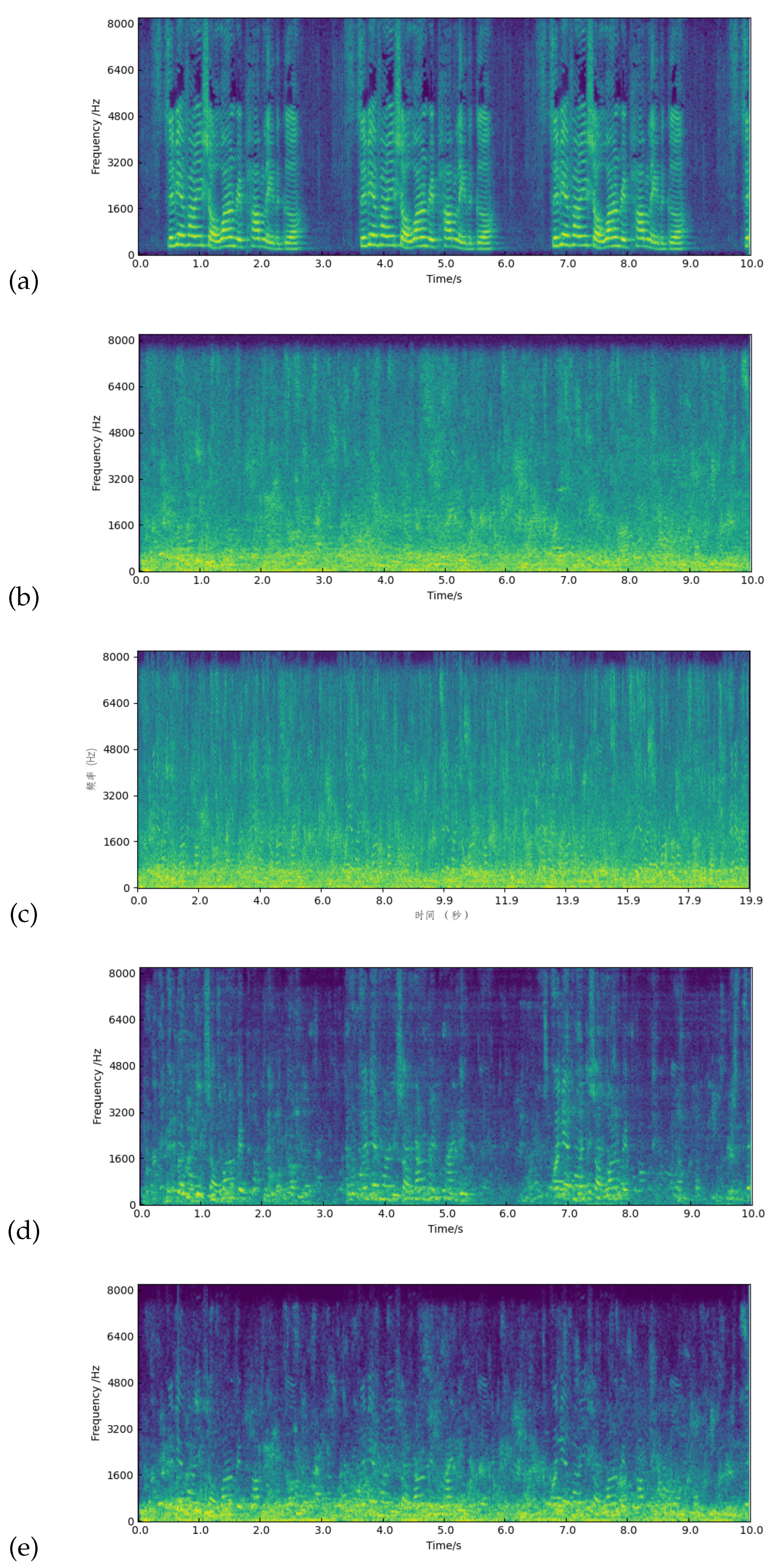
Figure 2.
Flow diagram of the proposed system.
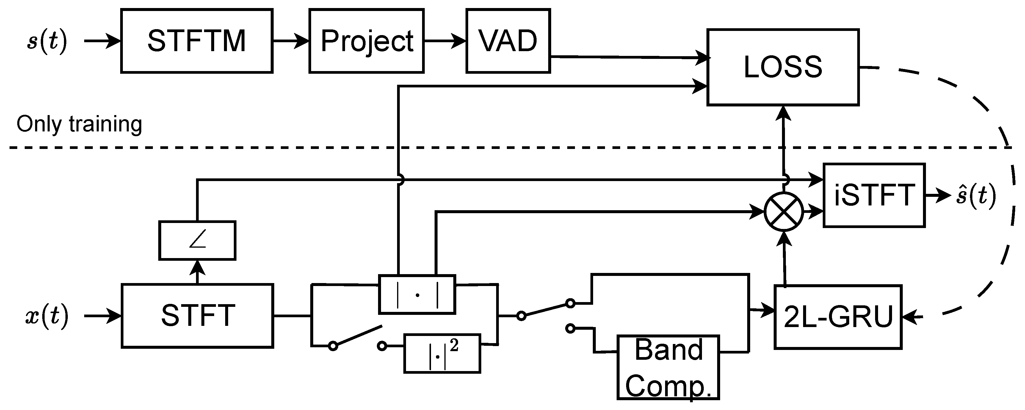
Figure 3.
Different filter bank. (a) Linear filter bank. (b) Bark filter bank. (c) Mel filter bank. (d) learnable filter bank.
Figure 3.
Different filter bank. (a) Linear filter bank. (b) Bark filter bank. (c) Mel filter bank. (d) learnable filter bank.
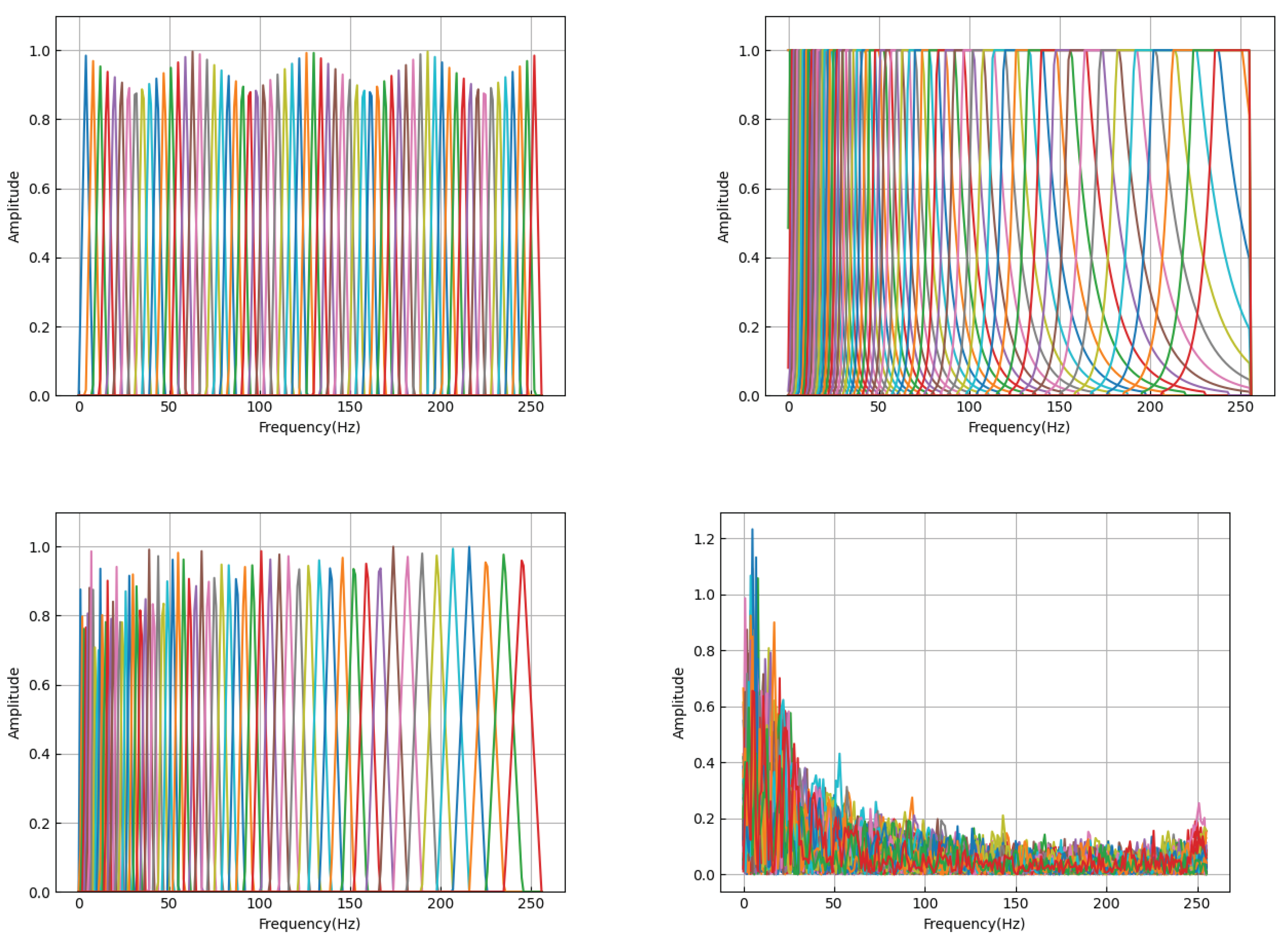

Table 1.
MCU Fixed-Point Integer Computing Performance Estimation.
| MCU | CoreMark | Inference Delay (ms) | Computing Capability (MMACs/s) |
|---|---|---|---|
| STM32H7 | 3223 | 51.95 | 230.85 |
| STM32F7 | 1082 | - | 77.5 |
| STM32L5 | 427 | - | 30.58 |
| STM32F4 | 565 | - | 40.46 |
| STM32L4 | - | 214 | 56.04 |
Table 2.
The type of QDNN.
| Type | Neuron Format | Computation | Complexity |
|---|---|---|---|
| T1 [30,31] | |||
| T1 [32,33,34] | |||
| T2 [35] | |||
| T3 [36] | |||
| T4 [37] | r | ||
| T1&2 [38] | |||
| Ours |
Table 3.
Model comparison for speech enhancement and computational efficiency.
| Model Name | Model Params | Comp. Speed | Computation Type |
|---|---|---|---|
| noisy | - | - | - |
| Fullsubnet+ [51] | 8.60M | 61.2 GMACs/s | Desktop Streaming |
| DCCRN [14] | 3.70M | 13.5 GMACs/s | Desktop Streaming |
| DPTNet [16] | 7.65M | 124.8 GMACs/s | Desktop Streaming |
| DCUNet [15] | 2.78M | 11.7 GMACs/s | Desktop Streaming |
| DPRNN [52] | 3.63M | 117.9 GMACs/s | Desktop Streaming |
| NSNet1 [17] | 1.32M | 0.17 GMACs/s | ARM Streaming |
| NSNet2 [18] | 2.68M | 0.54 GMACs/s | Desktop Streaming |
| RNN-Noise [13] | 0.87M | 0.044 GMACs/s | Edge Streaming |
| GRU-2l-256 | 0.86 M | 0.11 GMACs/s | ARM Streaming |
| GRU-2l-128-learn | 0.26 M | 0.033 GMACs/s | Edge Streaming |
Table 4.
Compare performance with other models in the DNS test set.
| Model Name | Low SNR STOI | High SNR STOI | Avg STOI | Low SNR PESQ | High SNR PESQ | Avg PESQ |
|---|---|---|---|---|---|---|
| Noisy | 1.398 | 2.125 | 1.710 | 0.598 | 0.867 | 0.713 |
| Fullsubnet+ | 1.913 | 3.255 | 2.488 | 0.705 | 0.918 | 0.796 |
| DPTNET | 1.717 | 2.904 | 2.226 | 0.660 | 0.906 | 0.765 |
| DPRNN | 1.711 | 2.880 | 2.212 | 0.659 | 0.907 | 0.765 |
| DCUNET | 1.650 | 2.871 | 2.173 | 0.671 | 0.905 | 0.771 |
| DCCRN | 1.544 | 2.705 | 2.041 | 0.618 | 0.894 | 0.736 |
| NSNet2 | 1.702 | 2.804 | 2.174 | 0.675 | 0.892 | 0.768 |
| NSNet1 | 1.421 | 2.369 | 1.827 | 0.499 | 0.728 | 0.597 |
| RNNNoise | 1.439 | 2.432 | 1.865 | 0.579 | 0.874 | 0.705 |
| GRU-2l-256 | 1.781 | 2.810 | 2.222 | 0.690 | 0.905 | 0.782 |
| GRU-2l-128-learn | 1.729 | 2.770 | 2.175 | 0.668 | 0.902 | 0.768 |
Table 5.
Compare performance with other models in the Speech Babble test set.
| Model Name | Low SNR STOI | High SNR STOI | Avg STOI | Low SNR PESQ | High SNR PESQ | Avg PESQ |
|---|---|---|---|---|---|---|
| Noisy | 1.486 | 2.106 | 1.752 | 0.535 | 0.883 | 0.684 |
| Fullsubnet+ | 1.490 | 2.864 | 2.079 | 0.533 | 0.912 | 0.695 |
| DPTNET | 1.305 | 1.195 | 1.258 | 0.184 | 0.125 | 0.159 |
| DPRNN | 1.291 | 1.230 | 1.265 | 0.181 | 0.124 | 0.157 |
| DCUNET | 1.198 | 1.252 | 1.221 | 0.147 | 0.117 | 0.134 |
| DCCRN | 1.316 | 1.202 | 1.267 | 0.157 | 0.118 | 0.140 |
| NSNet2 | 1.426 | 2.527 | 1.898 | 0.528 | 0.892 | 0.684 |
| NSNet1 | 1.401 | 2.337 | 1.802 | 0.424 | 0.754 | 0.566 |
| RNNNoise | 1.500 | 2.493 | 1.925 | 0.504 | 0.903 | 0.675 |
| GRU-2l-256 | 1.446 | 2.403 | 1.856 | 0.524 | 0.893 | 0.682 |
| GRU-2l-128-learn | 1.429 | 2.356 | 1.826 | 0.515 | 0.889 | 0.675 |
Table 6.
Compare performance with other models in the VCTK test set.
| Model Name | Low SNR STOI | High SNR STOI | Avg STOI | Low SNR PESQ | High SNR PESQ | Avg PESQ |
|---|---|---|---|---|---|---|
| Noisy | 1.407 | 2.265 | 1.774 | 0.586 | 0.811 | 0.683 |
| Fullsubnet+ | 1.982 | 3.324 | 2.557 | 0.642 | 0.858 | 0.735 |
| DPTNET | 1.913 | 3.139 | 2.439 | 0.636 | 0.859 | 0.732 |
| DPRNN | 1.935 | 3.158 | 2.460 | 0.627 | 0.862 | 0.728 |
| DCUNET | 1.788 | 2.989 | 2.303 | 0.621 | 0.850 | 0.720 |
| DCCRN | 1.692 | 2.930 | 2.223 | 0.567 | 0.839 | 0.683 |
| Nsnet2 | 1.799 | 3.018 | 2.321 | 0.632 | 0.853 | 0.726 |
| Nsnet1 | 1.542 | 2.693 | 2.035 | 0.475 | 0.690 | 0.567 |
| RNNoise | 1.547 | 2.693 | 2.038 | 0.575 | 0.835 | 0.687 |
| GRU-2l-256 | 1.641 | 2.668 | 2.081 | 0.571 | 0.817 | 0.676 |
| GRU-2l-128-learn | 1.770 | 2.749 | 2.189 | 0.610 | 0.840 | 0.709 |
Table 7.
Impact of band merging method on model performance on the DNS test set
| Model Name | Low SNR STOI | High SNR STOI | Avg STOI | Low SNR PESQ | High SNR PESQ | Avg PESQ |
|---|---|---|---|---|---|---|
| Noisy | 1.398 | 2.125 | 1.710 | 0.598 | 0.867 | 0.713 |
| Nolog-Noisy2 | 1.377 | 2.113 | 1.692 | 0.460 | 0.764 | 0.590 |
| Log-Noisy2 | 1.653 | 2.678 | 2.092 | 0.668 | 0.894 | 0.765 |
| Log-Noisy | 1.656 | 2.550 | 2.039 | 0.653 | 0.885 | 0.752 |
| Log-Noise_Noisy | 1.578 | 2.680 | 2.050 | 0.648 | 0.895 | 0.754 |
| Log-Noisy2_Noisy | 1.729 | 2.770 | 2.175 | 0.668 | 0.902 | 0.768 |
Table 8.
Impact of band merging method on model performance on the Speech Babble test set
| Model Name | Low SNR STOI | High SNR STOI | Avg STOI | Low SNR PESQ | High SNR PESQ | Avg PESQ |
|---|---|---|---|---|---|---|
| Noisy | 1.486 | 2.106 | 1.752 | 0.535 | 0.883 | 0.684 |
| Nolog-Noisy2 | 1.327 | 1.982 | 1.608 | 0.275 | 0.776 | 0.490 |
| Log-Noisy2 | 1.407 | 2.399 | 1.832 | 0.535 | 0.893 | 0.688 |
| Log-Noisy | 1.464 | 2.232 | 1.793 | 0.487 | 0.865 | 0.649 |
| Log-Noise_Noisy | 1.460 | 2.393 | 1.860 | 0.524 | 0.889 | 0.680 |
| Log-Noisy2_Noisy | 1.429 | 2.356 | 1.826 | 0.515 | 0.889 | 0.675 |
Table 9.
Impact of band merging method on model performance on the VCTK test set
| Model Name | Low SNR STOI | High SNR STOI | Avg STOI | Low SNR PESQ | High SNR PESQ | Avg PESQ |
|---|---|---|---|---|---|---|
| Noisy | 1.407 | 2.265 | 1.774 | 0.586 | 0.811 | 0.683 |
| Nolog-Noisy2 | 1.369 | 2.385 | 1.804 | 0.382 | 0.761 | 0.544 |
| Log-Noisy2 | 1.734 | 2.753 | 2.170 | 0.619 | 0.837 | 0.712 |
| Log-Noisy | 1.718 | 2.606 | 2.099 | 0.596 | 0.826 | 0.694 |
| Log-Noise_Noisy | 1.592 | 2.682 | 2.059 | 0.598 | 0.823 | 0.694 |
| Log-Noisy2_Noisy | 1.770 | 2.749 | 2.189 | 0.610 | 0.840 | 0.709 |
Table 10.
Impact of band merging method on model performance on the Speech Babble test set
| Model Name | Low SNR STOI | High SNR STOI | Avg STOI | Low SNR PESQ | High SNR PESQ | Avg PESQ |
|---|---|---|---|---|---|---|
| Noisy | 1.398 | 2.125 | 1.710 | 0.598 | 0.867 | 0.713 |
| Linear | 1.673 | 2.657 | 2.094 | 0.638 | 0.890 | 0.746 |
| Bark | 1.699 | 2.655 | 2.109 | 0.641 | 0.876 | 0.741 |
| Mel | 1.717 | 2.776 | 2.171 | 0.669 | 0.902 | 0.769 |
| Learn | 1.729 | 2.770 | 2.175 | 0.668 | 0.902 | 0.768 |
Table 11.
Impact of band merging method on model performance on the Speech Babble test set
| Model Name | Low SNR STOI | High SNR STOI | Avg STOI | Low SNR PESQ | High SNR PESQ | Avg PESQ |
|---|---|---|---|---|---|---|
| Noisy | 1.486 | 2.106 | 1.752 | 0.535 | 0.883 | 0.684 |
| Linear | 1.613 | 2.271 | 1.895 | 0.437 | 0.873 | 0.624 |
| Bark | 1.639 | 2.229 | 1.892 | 0.447 | 0.839 | 0.615 |
| Mel | 1.444 | 2.382 | 1.846 | 0.515 | 0.892 | 0.677 |
| Learn | 1.429 | 2.356 | 1.826 | 0.515 | 0.889 | 0.675 |
Table 12.
Impact of band merging method on model performance on the VCTK test set.
| Model Name | Low SNR STOI | High SNR STOI | Avg STOI | Low SNR PESQ | High SNR PESQ | Avg PESQ |
|---|---|---|---|---|---|---|
| Noisy | 1.407 | 2.265 | 1.774 | 0.586 | 0.811 | 0.683 |
| Linear | 1.721 | 2.674 | 2.130 | 0.576 | 0.832 | 0.686 |
| Bark | 1.723 | 2.706 | 2.144 | 0.577 | 0.824 | 0.683 |
| Mel | 1.729 | 2.729 | 2.158 | 0.610 | 0.838 | 0.708 |
| Learn | 1.770 | 2.749 | 2.189 | 0.610 | 0.840 | 0.709 |
Disclaimer/Publisher’s Note: The statements, opinions and data contained in all publications are solely those of the individual author(s) and contributor(s) and not of MDPI and/or the editor(s). MDPI and/or the editor(s) disclaim responsibility for any injury to people or property resulting from any ideas, methods, instructions or products referred to in the content. |
© 2024 by the authors. Licensee MDPI, Basel, Switzerland. This article is an open access article distributed under the terms and conditions of the Creative Commons Attribution (CC BY) license (http://creativecommons.org/licenses/by/4.0/).
Copyright: This open access article is published under a Creative Commons CC BY 4.0 license, which permit the free download, distribution, and reuse, provided that the author and preprint are cited in any reuse.


