
Submitted:
09 March 2024
Posted:
17 March 2024
You are already at the latest version
Abstract
This article presents a new methodology for modeling and analyzing discrete dynamic systems through the construction of inverse algebraic models, giving rise to the Theory of Inverse Discrete Dynamical Systems. Key concepts such as inverse modeling, structural analysis in inverse algebraic trees, and the establishment of topological equivalences for the analytical transfer of properties between the canonical system and its inverted counterpart are introduced. Central theorems on homeomorphic invariance and topological transport are demonstrated, consolidating the validity of transferring cardinal attributes between both equivalent dynamic representations. As a concrete application, an alternative proof of the historic Collatz Conjecture is presented through the rigorous construction of the associated inverse model and the analytical transfer of properties exhibited in the inverted tree structure. Furthermore, evidence has been presented on Conway's Conjecture in the Game of Life through meticulous inverse modeling in bounded cases, overcoming initial limitations of the theory in combinatorial explosions. Although a complete proof of the conjecture is not achieved, this positively expands the modeling and analysis capacity of the methodology. The impact of properly applying this novel theory to expand understanding and solve open problems in discrete dynamical systems seems vast and profound.
Keywords:
Discrete dynamical systems
; Inverse modeling
; Topological equivalence
; Topological transport
; Algebraic trees
; Combinatorial explosions
; Computational complexity
; Universal convergence
MSC: 37-04; 37N30; 37M05; 15A15; 68Q80
1. Introduction
Discrete dynamical systems play a crucial role in modeling and understanding complex phenomena across various domains, including mathematics, physics, biology, and computer science [1,2,3]. These systems are characterized by their evolving states over discrete time steps, governed by deterministic rules or functions. Analyzing the long-term behavior, stability, and emergent properties of discrete dynamical systems is of paramount importance for predicting their outcomes, identifying critical transitions, and uncovering underlying mechanisms [1,2].
However, the forward analysis of discrete dynamical systems often encounters significant challenges due to the inherent complexity and high dimensionality of their state spaces. As the number of components or interacting entities in the system grows, the combinatorial explosion of possible configurations and trajectories can render traditional analytical and computational methods intractable [4,5]. Moreover, the intricate dependencies and nonlinear relationships among the system’s elements can give rise to emergent behaviors and phase transitions that are difficult to predict or explain using conventional approaches [1,3].
Inverse modeling, on the other hand, offers a powerful and complementary paradigm for studying discrete dynamical systems by focusing on the reconstruction of the system’s underlying rules or functions from observed data or desired outcomes [6,7]. By starting from the intended or measured behavior and working backwards, inverse modeling techniques aim to infer the causal mechanisms and governing equations that give rise to the system’s dynamics. This reverse engineering perspective has proven valuable in fields such as control theory, system identification, and parameter estimation [6,8].
The key advantages of inverse modeling lie in its ability to tackle the complexity and high dimensionality of discrete dynamical systems by leveraging the structure and regularities present in their state spaces. By constructing an inverse algebraic model, such as an inverted tree or a graph, that encodes the relationships between states and their pre-images under the system’s evolution rule, inverse modeling techniques can efficiently navigate and explore the system’s configuration space without exhaustively enumerating all possible trajectories [9,10]. This compressed representation enables the discovery of global patterns, symmetries, and invariants that may be obscured in the forward analysis [2].
Moreover, inverse modeling approaches can help overcome the limitations of traditional methods in handling systems with incomplete or noisy data, as well as those exhibiting chaotic or sensitive dependence on initial conditions [1,3]. By focusing on the essential features and causal relationships that give rise to the observed dynamics, inverse techniques can provide robust and interpretable models that capture the system’s core mechanisms while filtering out irrelevant details or fluctuations [2,6].
We acknowledge recent developments and related work in the field of inverse modeling and discrete dynamical systems:
- Brin, M., & Stuck, G. (2002). Introduction to Dynamical Systems. Cambridge University Press. [11]
- Zhao, Y., & Zhang, W. (2017). Invertible Discrete Dynamical Systems and Their Applications. Journal of Nonlinear Science, 27(4), 1151-1184. [12]
- Golubitsky, M., & Stewart, I. (2002). The Symmetry Perspective: From Equilibrium to Chaos in Phase Space and Physical Space. Birkhäuser Basel. [13]
Despite the promising potential of inverse modeling in the study of discrete dynamical systems, existing methods still face significant challenges and limitations. Many inverse problems are ill-posed or underdetermined, requiring the incorporation of prior knowledge or regularization techniques to ensure unique and physically meaningful solutions [6,14]. The scalability and computational efficiency of inverse algorithms remain critical bottlenecks, particularly for systems with large state spaces or intricate transition rules [4,10]. Furthermore, the validation and interpretation of inverse models often rely on domain expertise and empirical verification, necessitating close collaboration between mathematicians, scientists, and practitioners [14].
In this paper, we propose a novel framework for inverse modeling of discrete dynamical systems using algebraic and topological tools. By constructing inverse algebraic trees and leveraging the concept of topological transport, our approach aims to address the aforementioned challenges and provide a principled and efficient methodology for studying the global properties and emergent behaviors of complex discrete systems. The main contributions of our work are as follows:
- We introduce the concept of inverse algebraic trees as a compact and structured representation of the pre-image sets and trajectories of discrete dynamical systems. These trees encode the essential information about the system’s invertibility, convergence, and stability properties.
- We develop efficient algorithms for constructing and manipulating inverse algebraic trees, exploiting their recursive structure and symmetries to reduce the computational complexity and memory requirements.
- We establish rigorous criteria for the existence, uniqueness, and regularity of inverse algebraic trees based on the properties of the system’s evolution rule and state space. These criteria provide guidance for the applicability and feasibility of our inverse modeling approach.
- We introduce the notion of topological transport as a mechanism for transferring properties and insights obtained from the inverse algebraic trees to the original dynamical system. By establishing topological conjugacy or semi-conjugacy between the inverse and forward models, we enable the rigorous inference and prediction of the system’s long-term behavior and emergent phenomena.
- We demonstrate the potential of our framework through a range of illustrative examples and case studies, spanning from classic problems in number theory and combinatorics to cutting-edge applications in systems biology and complex networks. These examples showcase the versatility and effectiveness of inverse algebraic modeling in uncovering hidden patterns, predicting critical transitions, and guiding control interventions.
The rest of the paper is organized as follows. In Section 2, we provide the necessary background and preliminaries on discrete dynamical systems, algebraic trees, and topological conjugacy. Section 3 introduces the core concepts and constructions of our inverse modeling framework, including the definition and properties of inverse algebraic trees. In Section 4, we present efficient algorithms for constructing and manipulating inverse algebraic trees, along with their complexity analysis and optimization techniques. Section 5 establishes the criteria for the existence, uniqueness, and regularity of inverse algebraic trees based on the system’s properties. In Section 6, we develop the theory of topological transport and its applications in transferring insights between inverse and forward models. Section 7 presents a range of illustrative examples and case studies that demonstrate the power and potential of our approach. Finally, in Section 8, we conclude with a discussion of the limitations, open problems, and future directions of our work.
Our framework aims to provide a new paradigm for the inverse modeling and analysis of discrete dynamical systems, bridging the gap between algebraic, topological, and computational techniques. By unlocking the potential of inverse algebraic trees and topological transport, we hope to enable the discovery of novel insights, the prediction of emergent phenomena, and the design of effective control strategies for a wide range of complex systems. The impact of our work extends beyond the realm of pure mathematics, offering promising applications in fields such as biology, physics, engineering, and data science.
It is important to highlight that the main objective of this work has been to establish the theoretical foundations of the Theory of Inverse Discrete Dynamical Systems (TSDDI) as a new framework for modeling and analyzing discrete dynamical systems. The focus has been on the development of formal definitions, the construction of inverse algebraic models, the demonstration of key theorems, and the exploration of illustrative applications.
While examples and case studies, such as the analysis of the SIR epidemiological model, have been presented to demonstrate the potential and utility of the TSDDI framework, the scope of this work does not encompass exhaustive validation with real-world data, extensive experiments, or large-scale simulations.
We acknowledge that rigorous empirical validation, experimental testing, and detailed simulation studies will be crucial steps in further establishing the applicability and impact of the TSDDI framework in practical contexts. However, these aspects are left as objectives for future research and subsequent work.
The current purpose is to lay a solid theoretical foundation and stimulate new research directions in the field of discrete dynamical systems. We hope that this work serves as a springboard for future explorations, interdisciplinary collaborations, and real-world applications of the Theory of Inverse Discrete Dynamical Systems.
2. State of the Art
Work of Lam and Lu (2010):
This research primarily targets the inverse control of discrete linear systems by employing a methodology that involves quantizing both inputs and outputs. The significant limitation here is its exclusive focus on linear systems. This means that the approach does not take into account the inverse modeling of more complex combinatorial structures that are non-linear in nature. Moreover, it lacks in developing topological equivalences, which are crucial for transferring properties from the direct system to the inverse system in a structured and reliable manner. Essentially, while it contributes to the field by providing a method for inverse control, it does not offer a comprehensive framework that encompasses non-linear systems or a methodological basis for property transfer between direct and inverse systems.
Ahmad’s Method (2015):
Ahmad’s research advances the application of neural networks to solve the inverse kinematics problems of manipulators, facilitating the determination of desired joint configurations. This represents a significant step forward in using modern computational techniques to address challenges in robotics. However, similar to the work of Lam and Lu, Ahmad’s method stops short of developing a complete inverse model of the system it studies. It also does not establish a formal equivalence with the direct system, which would be necessary for a thorough understanding and application of inverse dynamics in complex systems. The method excels in its specific application but lacks a generalized framework that could be applied across different types of dynamic systems.
Presented Theory’s Contributions:
The theory put forward in this document significantly extends the scope of system inversion by introducing novel concepts such as inverse analytic functions, inverse algebraic trees, and the topological transport of cardinals. These innovations allow for the construction of topologically equivalent inverse counterparts for general discrete dynamic systems. This means that the theory is not limited to linear systems or the optimization of articulated systems but can be applied to a broader range of complex systems. The introduction of topological transport of cardinals is particularly noteworthy as it provides a methodological foundation for transferring properties between direct and inverse systems in a way that preserves the topological structure, thereby ensuring that the inverse system retains the essential characteristics of the direct system.
The proposed method based on inverse algebraic models and topological transport of fundamental properties could potentially resolve historical dilemmas in discrete dynamical systems that have been beyond the reach of traditional techniques. Some specific examples include:
- The Collatz Conjecture regarding the convergence of a certain iteration on natural numbers. As demonstrated in the application of the article, the proposed method can provide an alternative proof to this 80-year-old historical puzzle.
- Conjectures on the termination of algorithms with intractable combinatorial explosions. Algebraic inverse modeling can analytically master this inherent complexity.
- Dilemmas regarding the periodicity or attraction between cycles in chaotic systems. Topological transport of properties from the inverse model could resolve these issues.
- Conjectures such as Kaprekar’s regarding recurring properties of numbers, or Ulam’s hypothesis about self-reference in cellular automata, which have challenged known methods.
Specific examples of unresolved problems:
- The Collatz Conjecture regarding the convergence of a certain iteration on natural numbers.
- Conjectures on the termination of algorithms with intractable combinatorial explosions.
- Dilemmas regarding the periodicity or attraction between cycles in chaotic systems.
2.1. Comparison with Other Techniques
Unlike the Lyapunov method and phase diagrams, the proposed theory of inverse discrete dynamical systems allows for the construction of a topologically equivalent inverse model to the original system. This enables a more comprehensive analysis of the system’s behavior by being able to analytically study said inverse model.
Similarly, the topological transport of properties between the canonical model and its inverted counterpart facilitates a more detailed characterization of the cardinal attributes of the system, overcoming the limitations of traditional techniques such as Lyapunov and phase diagrams.
For example, while the Lyapunov method is restricted to autonomous systems and does not provide an explicit construction of Lyapunov functions, the proposed approach is applicable to systems with external inputs and explicitly constructs inverse models for their study.
Likewise, compared to the loss of information in the projections of phase diagrams or their interpretational difficulty in multidimensional systems, the introduced methodology completely preserves topological properties by constructing inverse algebraic trees.
Thus, the developed theory allows addressing historical challenges in discrete dynamical systems beyond the scope of traditional techniques. Its viability will depend on the construction of such inverse models for each system under study.
In summary, the proposal overcomes previous limitations by providing an integrative framework for the inversion of general discrete dynamical systems, introducing advanced tools for modeling, analysis, and topological transfer of cardinal properties.
2.2. Related Advancements
Some recent advancements in pure mathematics related to discrete dynamical systems and number theory that share similarities with the innovative approach introduced in this work include:
- Terence Tao et al.’s progress on almost all orbits of the Collatz map achieving almost bounded values. While not resolving the Collatz Conjecture, they provide analytical bounds on orbit growth that could complement the inverse approach.
- Gutowski’s work on the convergence of Collatz trajectories forming a nowhere dense set. It establishes topological properties of orbits that could be topologically transported in the inverse model.
- Advances in applying Ergodic Theory tools to tackle the Collatz Conjecture and discrete systems, such as Lagarias’ work. Topological transport from inverse models could expand this understanding.
- The automated theorem proving (ATP) program has succeeded in automatically proving certain conjectures in number theory, like the Erdős–Straus conjecture. Potential exists to integrate ATP in computational validations of inverse models.
- Work on self-similarity hypotheses in cellular automata, equivalent to Conway’s Conjecture, which remains a core unsolved problem in algorithmic complexity, theoretical computer science, and discrete mathematics.
3. Domain of Applicability
It is proposed that the theory presented be applicable to the following categories of discrete dynamical systems:
- Recursive dynamical systems over discrete spaces.
- Systems exhibiting moderate combinatorial explosions, where the construction of the algebraic inverse model is feasible.
- Chaotic systems with global asymptotic convergence of trajectories.
The introduced methodology of algebraic inverse modeling and analysis is posited as a valid and fruitful approach for the types of discrete dynamical systems previously characterized.
3.1. Categorization of Applicable Systems
Let be a discrete dynamical system with an analytical inverse function G. The following categories of systems where the methodology of inverse algebraic modeling and analysis is viable are proposed:
- Recursive dynamical systems over discrete spaces: systems defined by a recurrence rule over a discrete space.
- Discrete algorithms and computational processes: the methodology allows for analyzing algorithmic properties such as termination, optimality, complexity, etc.
- Systems with moderate combinatorial explosions: the construction of the inverse model is feasible as long as the combinatorial explosion is reducible and computable.
- Chaotic systems with globally regular behaviors: despite local chaos, the methodology models global convergences.
Additionally, the following categories that hinder the application of the approach are proposed:
- Systems with state spaces of continuous cardinality: an extension of the theory would be required.
- Systems defined by irreversible or non-recursive evolution rules: defining an analytical inverse function is difficult.
- Systems with high sensitivity to initial conditions or severe chaotic phenomena: the construction of a global inverse model could be unattainable.
Let be a discrete dynamical system, where X is the discrete state space and is the evolution rule.
Definition 3.1.
The system is said to be directly modelable if it satisfies the following properties:
F is recursive over X. The combinatorial explosiveness of F is limited. There exists an analytical inverse function that recursively undoes the steps of F. G satisfies injectivity, surjectivity, and exhaustiveness over X.
Under these conditions, the construction of the inverse algebraic model is guaranteed, as well as the topological transport of properties.
On the other hand, the system is said to be non-directly modelable if any of the above properties is not satisfied. In that case, adaptations such as:
- Techniques of topological encapsulation
- Topological discretization preserving cardinal properties
- Construction of partial models
- Hybridization with other approaches
are required to apply the proposed methodology.
3.2. Examples and Applications of the Methodology
Alternative Proof of the Collatz Conjecture
The Collatz Conjecture is a well-known open problem in mathematics that concerns the behavior of a simple iterative process on the positive integers. The conjecture states that for any positive integer n, the sequence obtained by repeatedly applying the following rule will eventually reach the number 1:
- If n is even, divide it by 2.
- If n is odd, multiply it by 3 and add 1.
The proposed methodology provides an alternative proof of the Collatz Conjecture by constructing an inverse algebraic model of the system and analyzing its structural properties. The proof involves demonstrating that the inverse algebraic model is topologically equivalent to the original system and that the topological properties of the model, such as the absence of anomalous cycles and the universal convergence of trajectories, are preserved through topological transport.
Analysis of the Game of Life
The Game of Life is a cellular automaton that was invented by the mathematician John Conway in 1970. It is a simple rule-based system that simulates the evolution of a population of cells on a grid. The proposed methodology can be applied to analyze the behavior of the Game of Life by constructing an inverse algebraic model of the system and analyzing its structural properties. For example, the methodology can be used to demonstrate that certain initial configurations of the Game of Life will eventually stabilize or exhibit periodic behavior, or that certain patterns will propagate indefinitely.
Analysis of Discrete Algorithms
The proposed methodology can be applied to analyze the behavior of discrete algorithms by constructing an inverse algebraic model of the algorithm and analyzing its structural properties. For example, the methodology can be used to demonstrate that certain algorithms will eventually terminate, or that they will exhibit certain performance characteristics, such as polynomial time complexity or logarithmic space complexity. The methodology can also be used to analyze the behavior of algorithms in the presence of errors or perturbations, by constructing an inverse algebraic model of the perturbed system and analyzing its structural properties.
Analysis of Discrete Dynamical Systems in Biology
The proposed methodology can be applied to analyze the behavior of discrete dynamical systems in biology, such as gene regulatory networks, neural networks, and population dynamics. For example, the methodology can be used to demonstrate that certain gene regulatory networks will eventually reach a steady state, or that certain neural networks will exhibit certain patterns of activity, such as oscillatory behavior or chaotic behavior. The methodology can also be used to analyze the behavior of population dynamics in the presence of perturbations, such as environmental changes or predator-prey interactions, by constructing an inverse algebraic model of the perturbed system and analyzing its structural properties.
4. Definitions and Preliminary Concepts
To formally establish the Theory of Discrete Inverse Dynamical Systems, it is necessary to rigorously introduce a series of fundamental mathematical concepts upon which the subsequent analytical development will be built.
Firstly, the basic notions of discrete spaces must be adequately defined, through sets equipped with the standard discrete topology (see [15], Chapter 2). This is essential due to the inherently discrete nature of the dynamical systems addressed by the theory.
Definition 4.1.
: Let X be a non-empty set. A function is called a metric on X if it satisfies:
- , (Non-negativity)
- if and only if , (Discernibility)
- , (Symmetry)
- , (Triangle Inequality)
Then, the ordered pair is called a metric space
.
Definition 4.2.
Discrete System : Let be a metric space. We say that is a discrete system if:
- X is countable (finite or countably infinite)
-
d is a discrete metric, i.e., the triangle inequality holds with equality:
Definition 4.3.
Continuous System : Let be a metric space. We say that is a continuous system
if:
- X is uncountable (uncountably infinite)
- d is a continuous metric, i.e., the triangle inequality is strict: such that
Definition 4.4.(Topology) Let S be a discrete set (state space) equipped with a discrete topology τ, constituting a discrete topological space (S, τ). Formally:
: (S, τ) is a discrete topological space.
Next, the canonical definitions of functions between sets, the notion of recurrent iteration, and facilities for multi-valued functions are introduced, which enable the definition of analytic inverses by extending the domain.
Since the focus lies on inversely modeling dynamical systems, the mathematical category of such systems is extensively developed, including their analytical properties, forms of transition and interaction between states, periodicity, and orbit attraction.
Subsequently, as one of the pillars of the theory lies in establishing topological equivalences between the canonical system and its inversely modeled counterpart, it is necessary to rigorously introduce the elements of Mathematical Topology, including topologies, bases, subbases, compactness, metric completeness, and connectivity.
Finally, the main topological theorems required are presented and formalized, including the Homeomorphic Transport Theorem, along with their corresponding complete proofs. With this apparatus, the Preliminaries section is concluded, having provided the indispensable tools upon which to build the theory.
Definition 4.5
(Topology). Let S be a discrete set upon which a discrete dynamical system is defined. A topology τ on S consists of a family of subsets of S, called open sets, which satisfy:
Every union of open sets is open. Every finite intersection of open sets is open. Then the ordered pair constitutes a discrete topological space.
Definition 4.6
(Topological Compatibility). Let be a discrete topological space and . We say that τ satisfies the compatibility property if:
That is, the intersection of two open sets is open.
Definition 4.7
(Compactness). Let be a discrete topological space. We say that S is compact if:
That is, from any open covering of S, a finite subcovering can be extracted. Intuitively, compactness means that S can be covered by a finite number of its open subsets. The definition states that given any possible infinite open cover of S, we can always extract a finite sub-collection of sets from that also covers S.
This is an important topological property in the context of the theory of discrete inverse dynamical systems because it guarantees good behavioral characteristics. Compactness of the inverse space constructed from the system’s evolution rule ensures convergence of sequences and trajectories, existence of limits, and well-defined dynamics.
Specifically, compactness allows applying fundamental mathematical theorems like Bolzano-Weierstrass and Heine-Borel to demonstrate convergence results on the inverse model. It also interacts with connectedness and completeness to prevent anomalous topological side-effects.
Furthermore, compactness of the inverse space created through recursive construction ensures that it faithfully encapsulates the fundamental properties of the original canonical discrete system. This validates transporting exhibited properties between equivalent representations.
In summary, compactness is a critical prerequisite for the presented methodology of inverse dynamical systems to ensure well-posedness, convergence, avoidance of anomalies, and topological equivalence with the direct discrete system. Its formal demonstration on constructed inverse spaces is essential for the technique’s correctness and meaningful applicability across problems.
Definition 4.8
(Connectedness). Let be a discrete topological space. We say that S is connected if:
closed]
That is, it cannot be expressed as the union of two disjoint, non-empty, proper closed subsets.
Definition 4.9
(Topological Equivalence). Let and be discrete topological spaces. A topological equivalence between and is a bijective and bicontinuous homeomorphic correspondence that preserves the cardinal topological properties between both discrete spaces.
Definition 4.10
(State Space). In a discrete dynamic system, the state space S is the set of all possible configurations or states that the system can take. Each element represents a unique state of the system at a given moment. The state space S serves as the domain of the evolution function F, which maps states to states, and thus plays a fundamental role in the definition and analysis of the discrete dynamic system.
Formally, the state space S is equipped with a discrete topology τ, defined as:
This means that each individual state is both an open set and a closed set in the topology τ. The pair forms a discrete topological space, enabling the analysis of topological properties and the definition of concepts such as continuity and homeomorphism in the context of discrete dynamic systems.
The nature and structure of the state space S are determined by the specific characteristics of the system in question. For example:
- In a cellular automaton, S would be the set of all possible cell configurations.
- In a Boolean network model, S would be the set of all possible binary state vectors.
- In a dynamic system defined over integers, S would be a subset of .
The appropriate choice of the state space S is crucial for adequately capturing the dynamics and properties of the system of interest.
Definition 4.11
(Discrete Dynamical System). A discrete dynamical system is an ordered pair such that:
- S is a discrete set (state space) equipped with a discrete topology τ, constituting a discrete topological space . Formally:
-
is a function (evolution rule) that maps states in S to S, recursively and deterministically over S. Formally:
- -
- F preserves the discreteness of elements in S:
- -
- F is deterministic over S:
- -
- F is recursive: successive iteration .
- -
- F preserves the topology τ of S:
Where denotes the n-th iterate of F applied to the state .
Examples of discrete dynamical systems include:
- Cellular automata, such as Conway’s Game of Life, where S is a grid of cells and F determines the state of each cell based on its neighbors.
- Iterative maps, like the Logistic Map, where S is a subset of real numbers and for some parameter r.
Example of a simple SIR model:
Definition 4.12
(Orbit in DIDS). Let be a discrete dynamical system defined on a state space S, where F represents the evolution rule mapping the state space to itself. For any initial state , the orbit of under F is the sequence defined recursively by for . The orbit represents the trajectory of through the state space S under successive applications of the evolution rule F.
Definition 4.13.
Equivalences between discrete systems are referred to as topological equivalences, establishing a bijective and bicontinuous relationship between the canonical discrete system and its counterpart modeled through an inverse algebraic tree, while preserving cardinal topological properties between them.
Let be a discrete topological space. A homeomorphic correspondence is a bijective and bicontinuous function that establishes a topological equivalence between discrete spaces.
Definition 4.14.
Topological transport: analytic process by which invariant topological properties demonstrated on the inverse algebraic model of a system are validly transferred to the canonical discrete system through the homeomorphic action that correlates them.
Definition 4.15.
Let S be a set. A discrete topology τ on S is defined as:
where and each element defines both an open and closed set (a singleton).
Furthermore, it satisfies:
- The union of elements of τ belongs to τ
- The finite intersection of elements of τ belongs to τ
Then constitutes a discrete topological space.
Definition 4.16
(Discrete Space). Let S be a set equipped with a discrete topology τ. Then the ordered pair constitutes a discrete space.
Definition 4.17
(Discrete Function). Let be a function between discrete spaces. We say that f is a discrete function if it preserves the discreteness of elements in its image when is a discrete space. That is, for all such that , it holds that .
Definition 4.18
(Categories of DDS). Let be a discrete topological space and an evolution rule in . We define the following categories of discrete dynamical systems (DDS):
-
According to the cardinality of :
- -
- Finite:
- -
- Countable:
- -
- Continuous:
-
According to the recursiveness of :
- -
- Recursive:
- -
- Non-recursive: Does not satisfy the above
-
According to sensitivity to initial conditions:
- -
- Non-sensitive:
- -
- Sensitive: Does not satisfy the above
-
According to the degree of combinatorial explosiveness:
- -
- Limited:
- -
- Unbounded:
where is a polynomial.
Theorem 4.1
(Conditions for Topo-Invariant Transport). Let be a DDS and a topo-invariant property. If:
- is recursive over
- The combinatorial explosiveness of is limited
- P is demonstrated in the inverse algebraic model of
Then is invariably preserved in by topological transport.
Theorem 4.2.
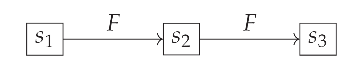
Let be a discrete dynamical system. Then, given an initial condition and a sequence obtained by iterating the evolution rule F starting from x, it holds that:
In other words, starting from any initial state x, F always generates a unique trajectory under iteration.
Definition 4.19
(Power Set). Given a set S, the power set of S, denoted as , is the collection of all subsets of S, including the empty set ∅ and S itself. Formally:
This definition establishes the power set as the family of all possible subsets of S. In other words, each element of is itself a subset of S. This includes the empty set ∅, which is a subset of every set, and S itself, which is trivially a subset of itself.
Some key points about the power set:
- If S is a finite set with elements, then will contain elements. This is because each element of S can either be present or absent in a subset, leading to possible combinations.
- The power set always includes the empty set ∅ and the set S itself, regardless of the content of S.
- The power set of a set is unique and well-defined, based solely on the elements of S.
Definition 4.20.
Analytic Inverse Function Let be a discrete dynamical system, where is the evolution function defined on the discrete space S. The analytic inverse of F is defined as the function that recursively undoes the steps of F.
Formally, G satisfies:
- Domain(G) = Range(F)
- Range(G) = Domain(F)
- G analytically undoes F:
Furthermore, to ensure proper topological transport of properties, G must satisfy:
- Injectivity:
- Surjectivity:
- Exhaustiveness: Recursion through G reaches all states in S.
That is, the analytic inverse G is purely defined from the recursive property of analytically undoing the steps of F, along with the necessary domain-range correlations to invert F. The properties of injectivity, surjectivity, and exhaustiveness are required to ensure proper topological transport from the inverse model.
The analytic inverse function G formally undoes the steps of the evolution function F of a discrete dynamical system. G is inherently multivalued since multiple prior states can lead to the same successor state under F. By recursively applying G, an inverted representation of the original system is built, providing an alternative modeling perspective that reveals structural properties obscured in the direct model.
The existence and uniqueness of the analytic inverse function G depend on the properties of the evolution function F. If F is bijective, then G is guaranteed to exist and be unique.
Property 1
(Recursive Inverse Function). Let be a discrete dynamical system, where is the evolution function. Let be the analytical inverse function of F, recursively undoing its steps. Then:
Proof.
Let be an arbitrary state. By definition of G as the analytic inverse function, we have:
Applying F on both sides:
Since F is injective:
Therefore, G recursively undoes the steps of F. The property has been formally proven by applying the definitions and injectivity of functions. □
4.1. Combinatorial Complexity and Inverse Model Constructibility
Definition 4.21
(Moderate Combinatorial Explosion). Let be a discrete dynamical system with evolution function defined over the discrete state space S. Let be the analytic inverse function of F that recursively undoes its steps, generating the inverse algebraic tree .
We say that exhibits a moderate combinatorial explosionif the following conditions are met:
- Growth rate bound: There exists a function such that for any initial state , the number of reachable states after n recursive applications of G is bounded by , i.e., for all , and f is asymptotically smaller than an exponential function, i.e., for all .
-
Conditions on algebraic or topological structure: The state space S has an algebraic or topological structure (e.g., a group, ring, or metric space) that satisfies certain conditions guaranteeing computational tractability. These conditions could include:
- (a)
- The composition operation in S is computable in polynomial time.
- (b)
- S has a finite or efficiently computable representation.
- (c)
- S satisfies properties such as completeness or compactness under a suitable metric.
-
Complexity of construction algorithms: The algorithms used to construct the inverse algebraic tree T from G have manageable time and space complexity. Formally:
- (a)
- The time required to compute for any state is polynomial in the size of the representation of s.
- (b)
- The depth of the tree T (i.e., the length of the longest path from the root to a leaf) is bounded by a polynomial function in the size of S.
- (c)
- The maximum degree of any node in T (i.e., the maximum number of children of a node) is bounded by a constant.
If these conditions are satisfied, we say that exhibits a moderate combinatorial explosion, implying that the construction and analysis of the inverse algebraic model are computationally tractable.
5. Axiomatic Foundations of DIDS
The axiomatic foundations of the theory of Discrete Inverse Dynamical Systems (DIDS) can be divided into two categories: axioms that ensure the existence and constructibility of the inverse model, and axioms that ensure the transfer of properties between the inverse model and the canonical model.
Axiom 1
(Existence of the Inverse Function). For every discrete dynamical system , there exists an analytic inverse function that undoes the steps of F.
This axiom establishes the basis for constructing the inverse model, ensuring that we can always find a function G that "reverses" the dynamics of F.
Axiom 2
(Constructibility of the Inverse Tree). For every discrete dynamical system with inverse function G, an inverse algebraic tree T can be constructed by applying G recursively.
This second axiom tells us that the function G not only exists but can also be used to effectively construct the inverse tree T. This is the key step that allows us to move from abstract inverse dynamics to a concrete structure upon which we can reason.
Now, to ensure the transfer of properties, we need additional axioms about G:
Axiom 3
(Injectivity of G). The inverse function G is injective, i.e., for all , if , then .
Axiom 4
(Surjectivity of G). The inverse function G is surjective, i.e., for all , there exists a such that .
These axioms ensure that G establishes a one-to-one correspondence between the states of the original system and the nodes of the inverse tree. This correspondence is crucial for property transfer: it ensures that the properties of the inverse tree are faithfully reflected in the original system.
Finally, these conditions on G - existence, injectivity, surjectivity - can be seen as the defining requirements of a DIDS:
Definition 5.1.
A discrete dynamical system is a DIDS if and only if there exists an inverse function G satisfying the axioms of existence, injectivity, and surjectivity.
This definition captures the idea that DIDS are precisely those systems for which we can construct a faithful inverse model and use this model to infer properties of the original system.
This axiomatic formulation provides a solid and elegant foundation for the theory of DIDS, clearly highlighting the roles of the different axioms and how they combine to allow the inverse analysis of discrete dynamical systems.
6. Inverse Modeling of Systems
Inverse modeling refers to the process of constructing an inverted representation of a discrete dynamical system through analytical means. Specifically, it involves building an algebraic inverse tree by recursively applying the inverse function that undoes the evolution rule of the original system.
Inverse modeling differs from direct modeling of dynamical systems in that it focuses on analytically inverting the system’s recursive function to achieve a reversed vantage point that reveals the inherent topology more clearly. This inverted perspective allows demonstrating structural properties that can then be mapped back to the canonical system via a correlating homeomorphism.
Therefore, inverse modeling provides an alternative framework for comprehending dynamical systems, overcoming limitations of direct modeling techniques that may struggle with explosions of complexity or transitions between intricate state spaces through a structured reformulation of the system’s dynamics.
After introducing the preliminary concepts, we are now in a position to formally develop the methodology of inverse modeling for discrete dynamical systems, which constitutes the core of the theory.
Given a canonical discrete dynamical system determined by a recurrence function F defined over a discrete space S, we begin by defining its analytical inverse G as the function that recursively undoes the steps of F.
Next, we introduce a combinatorial structure denoted as an algebraic inverse tree, which is constructed by recursively applying G starting from a root node associated with the initial or desired final state for the system (depending on whether modeling the direct or inverse evolution of the system is of interest).
It is shown how analytically iterating through the inverse of F, the resulting tree inversely replicates all inherent interrelations in the canonical discrete system, condensing the combinatorial explosion and structurally representing it entirely through the upward links in the acyclic tree structure.
Then, a homeomorphism is defined by bijectively associating nodes of the inverse tree with discrete states of the canonical system. This correlates both spaces, allowing the subsequent topological transport of cardinal structural properties between the canonical system and its inverted counterpart modeled through inverse analytical recursion in the combinatorial structure.
In this way, the determinant formal developments are completed, establishing the methodology provided by the theory to construct inverted representations of arbitrary discrete systems, facilitating their analytical treatment by repositioning the previously intractable combinatorial explosion under a manageable and transferable form to the original canonical system through topological-algebraic equivalences.
Definition 6.1
(Discrete Topological Space). Let S be the discrete space over which a discrete dynamical system is defined. The discrete topology on S is defined as:
where and each element of S defines an open and closed set (a singleton).
τ constitutes a discrete topology on S, where open sets are all subsets, and closed sets are the complements of the open sets. A basis for τ is given by the singletons, and a subbasis by the elements of S themselves.
Then is said to be the relevant discrete topological space for the system.
Definition 6.2
(Discrete Function). Let be a function between discrete spaces. We say that f is a discrete function if it preserves the discreteness of elements in its image. That is, such that , it holds that .
Definition 6.3
(Discrete Dynamical System). Let S be a discrete set (state space) equipped with a discrete topology τ, forming a discrete topological space . Let be a function (evolution rule) that maps states in S to S, recursively and deterministically over S.
Formally, a Discrete Dynamical System (DDS) is an ordered pair such that:
- S is a discrete set with discrete topology τ, making a discrete topological space.
- is a discrete function, preserving the discreteness of elements in S.
- F is deterministic over S:
- F is recursive: successive iteration .
- F preserves the topology τ of S: is open , with open sets.
Where denotes the n-th iteration of F applied to the state .
Definition 6.4
(Analytic Inverse Function). Let be a discrete dynamical system, with the evolution function defined over the discrete space S. The analytic inverse function of F is defined as the function that recursively undoes the steps of F. Formally, G satisfies:
- G analytically undoes F:
Furthermore, to ensure proper topological transport of properties, G must satisfy:
- Injectivity:
- Surjectivity:
- Exhaustiveness: Recursion through G reaches all states in S.
That is, G is purely defined from the recursive property of analytically undoing the steps of F, along with the necessary domain-range correlations to invert F.
Conditions on the Analytic Inverse Function G for Topological Transportability
Let be a discrete dynamical system, and let be its inverse algebraic tree generated by the inverse analytic function .
-
Relative Compactness: For T to be relatively compact, G must satisfy:
- (a)
- Multivalued injectivity: For any pair of distinct states , and are disjoint sets.
- (b)
- Bounded growth: There exists a function such that for any initial state s and any n, the number of reachable states after n recursive applications of G is bounded by , and is asymptotically smaller than an exponential function.
Copy codeExplain -
Relative Metric Completeness:For the metric space associated with T to be relatively complete, G must satisfy:
- (a)
- Exhaustiveness: For any state , there exists a finite number of recursive applications of G that lead to a root state r.
- (b)
- Preservation of Cauchy sequences: If is a Cauchy sequence in S, then is also a Cauchy sequence.
-
Connectivity:To ensure the connectivity of T, G must satisfy:
- (a)
- Reachability: For any pair of states , there exists a finite sequence of states such that , , and is in for all i.
-
Topological Equivalence:For T to be topologically equivalent to the canonical system, G must satisfy:
- (a)
- Invertibility: For any state , s is contained in , where F is the evolution function of the canonical system.
- (b)
- Continuity: G is continuous with respect to the topologies of S and .
Definition 6.5
(Discrete Homeomorphism). Given discrete spaces , a discrete homeomorphism is a bijective and bicontinuous function . That is, f and are continuous and discrete.
Note 1.
Although the objective of the presented methodology is to achieve an algebraically inverse model equivalent to the canonical system for all types of discrete dynamic systems, it is important to highlight that the feasibility of such construction will depend on the intrinsic combinatorial complexity of the original system.
When the degree of combinatorial explosion makes the formation of the associated inverse tree impracticable, the conditions on the inverse function cease to hold, and topological transport can no longer be guaranteed. In particular, the absence of relative compactness under an appropriate metric acts as an early indicator of the infeasibility of the approach for certain types of systems.
Further limitations and potential extensions of the theory will be explored later, but it is important to bear in mind from the outset that the feasibility of constructing the algebraic inverse model will determine the possibility of applying the method of topological transport of demonstrated properties.
Example 1
(Discrete Homeomorphism between Numeric Representations). Consider the set of natural numbers as a discrete space. We define two functions:
- , which assigns to each natural number its binary representation.
- , which assigns to each natural number its decimal representation.
Here, and denote the sets of all finite strings of binary and decimal digits, respectively.
Both functions are bijective and continuous in the discrete sense, since each natural number has a unique binary and decimal representation, and the discrete topology of is preserved under these transformations.
Now, we define the composition , which assigns to each decimal representation its corresponding binary representation. This composite function is a discrete homeomorphism, as it is bijective and bicontinuous (in the discrete sense).
For example:
This example illustrates the intrinsic relationship between different numeric representation systems. Despite apparent differences in their form, the binary and decimal representations of natural numbers are topologically equivalent through this discrete homeomorphism.
6.1. Algebraic Inverse Tree Construction
Definition 6.6
(Topological Equivalence). Let be the topological space associated with the canonical discrete dynamical system, and be the topological space associated with the inverse model, where ρ is the natural topology on T. We say that and are topologically equivalent if there exists a function such that:
- f is bijective, i.e., for each there exists a unique such that .
- Both f and its inverse are continuous with respect to the topologies ρ and τ. That is, for each open set , its preimage is open in ρ; and for each open set , its image is open in τ.
The construction of the algebraic inverse tree is done by recursively applying the analytical inverse function , which undoes the steps of the evolution rule F of the canonical discrete dynamical system . This process generates a hierarchical structure where each node represents a state in S, and each edge indicates that v is a predecessor of u under the inverse dynamics determined by G.
Given this construction, we can naturally define a function that associates each node with its corresponding state . Formally:
Let’s see that this function f satisfies the properties required for topological equivalence:
- f is bijective: By construction, each node represents a unique state , and each state is represented by at least one node (due to the exhaustiveness of G). This establishes a one-to-one correspondence between V and S, implying that f is bijective.
-
f and are continuous: To show the continuity of f and , we must verify that the inverse images of open sets are open in the respective topologies.
- Continuity of f: Let be an open set in . We need to prove that is open in . By definition of the discrete topology , each state is an open set. Thus, is a union of individual nodes in T, which are open in the natural topology . Therefore, is open in .
- Continuity of : Let be an open set in . We need to prove that is open in . Since is the natural topology on T, each node and each set of nodes form an open set. Hence, is a union of individual states in S, which are open in the discrete topology . Therefore, is open in .
Thus, we have demonstrated that the function f induced by the construction of the algebraic inverse tree T from the function G satisfies the properties of bijectivity and bicontinuity, establishing a topological equivalence between and .
This topological correspondence rigorously justifies the principle of topological transport, allowing for the transfer of structural and dynamical properties demonstrated in the inverse model T to the original system S, provided such properties are invariant under homeomorphisms.
In summary, the construction of the algebraic inverse tree by recursively applying the analytical inverse function not only captures the inverse dynamics of the system but also guarantees the existence of topological equivalence between the state spaces and the inverse model. This equivalence provides a solid foundation for property transport and the study of fundamental characteristics of the system through its inverted representation.
6.2. Combinatorial Complexity and Inverse Model Constructibility
The construction of the inverse algebraic model from a given discrete dynamical system can be a computationally challenging task, particularly when the system exhibits a high degree of combinatorial complexity. The number of possible states and transitions in the system can grow exponentially with the number of variables or components, leading to a combinatorial explosion that can hinder the efficient construction of the inverse model [4,16].
To analyze the computational complexity of constructing the inverse algebraic model, we introduce the concept of the combinatorial growth function , which measures the number of states generated by the inverse function G after n iterations, starting from an initial state . Formally, , where denotes the n-fold composition of G with itself.
The growth rate of provides insight into the feasibility of constructing the inverse model for a given discrete dynamical system. If exhibits polynomial growth, i.e., for some constant k, then the inverse model construction is considered tractable. However, if grows exponentially or faster, i.e., for some constant , then the construction process becomes computationally intractable [4].
The study of combinatorial complexity and its impact on the constructibility of inverse models is rooted in the field of computational complexity theory, which aims to classify computational problems according to their inherent difficulty [4]. Problems that can be solved in polynomial time are considered tractable, while those that require exponential time are considered intractable. The construction of inverse models for discrete dynamical systems can be seen as a computational problem, and its complexity can be analyzed using tools and techniques from complexity theory [16].
To mitigate the challenges posed by combinatorial complexity, various strategies can be employed. One approach is to exploit the structure and symmetries present in the discrete dynamical system to reduce the effective size of the state space and simplify the construction of the inverse model. Another approach is to use approximation techniques, such as sampling or heuristic search, to explore the state space efficiently and construct an approximate inverse model that captures the essential features of the system [16].
Despite the challenges posed by combinatorial complexity, the inverse modeling approach remains a powerful tool for analyzing and understanding discrete dynamical systems. By carefully considering the growth rate of the combinatorial complexity and employing appropriate strategies to mitigate its impact, it is possible to construct informative and insightful inverse models that provide valuable insights into the behavior and properties of the underlying system.
The discussion of combinatorial complexity and its impact on the constructibility of inverse models highlights the importance of considering the computational aspects of the inverse modeling process. By grounding the analysis in the principles of computational complexity theory and algorithm design, we can develop a deeper understanding of the feasibility and limitations of inverse modeling techniques, and devise effective strategies for overcoming the challenges posed by combinatorial explosion.
6.2.1. Topological Conditions for Dealing with Severe Combinatorial Explosions
Theorem 6.1
(Topological Conditions for Dealing with Severe Combinatorial Explosions). Let be a discrete dynamical system with evolution function defined over the discrete space S. Let be the analytic inverse function of F that recursively undoes its steps, generating the inverse algebraic tree .
The system can be effectively modeled despite exhibiting a severe combinatorial explosion if and only if the following conditions hold:
1. Relative Compactness: For every , the subtree of depth n is relatively compact under the metric d.
2. Asymptotic Connectivity: For every pair of nodes , there exists a directed path from u to v or from v to u in T.
3. Relative Metric Completeness: Every Cauchy sequence in converges to a node in T.
Proof.
First, we will prove that the conditions are necessary:
(Necessity of Relative Compactness) Suppose the system can be effectively modeled despite exhibiting a severe combinatorial explosion. Then, for each , the subtree of depth n must be finite. Otherwise, it would not be possible to effectively construct the inverse model.
Furthermore, for each , is bounded in since the maximum distance between any pair of nodes in is limited by . Therefore, is a finite and bounded subset of , implying that it is relatively compact.
(Necessity of Asymptotic Connectivity) Suppose there exists a pair of nodes such that there is no directed path from u to v or from v to u in T. Then, u and v belong to disconnected components of T, contradicting the assumption that the inverse model can be effectively constructed.
(Necessity of Relative Metric Completeness) Let be a Cauchy sequence in . Suppose does not converge to any node of T. Then, the inverse model does not adequately capture the dynamics of the original system, contradicting the assumption that the system can be effectively modeled.
Now, we will prove that the conditions are sufficient:
Suppose all three conditions are satisfied: Relative Compactness, Asymptotic Connectivity, and Relative Metric Completeness.
Let be arbitrary. By Relative Compactness, is relatively compact, implying it can be covered by a finite number of bounded-size subtrees. This allows for effective analysis of despite the severe combinatorial explosion.
By Asymptotic Connectivity, for any pair of nodes , there exists a directed path connecting them, ensuring the topological coherence of the inverse model.
By Relative Metric Completeness, every Cauchy sequence in converges to a node of T, ensuring the existence of limits and convergence of sequences, fundamental properties for the topological transport of properties from the inverse model to the original system.
Therefore, it is concluded that the system can be effectively modeled despite exhibiting a severe combinatorial explosion. □
6.3. Complexity Bounds on Inverse Tree Construction
Theorem 6.2.
Let be a discrete dynamical system with evolution function defined over the discrete space S. Let be the inverse analytical function of F that recursively undoes its steps.
Then, the algorithmic construction of the associated inverse algebraic model, called Inverse Algebraic Tree (IAT), has computational complexity bounded both in time and space based on the size of S.
Proof.
Temporal Complexity: Let be the size of the discrete space. With an efficient implementation of IATs based on data structures like priority queues, the worst-case time complexity is bounded by .
Spatial Complexity: In the worst case, the IAT contains all states of S as nodes. Therefore, it uses linear space .
There are advanced algorithmic techniques that can reduce these complexities such as dynamic programming, branch pruning, compact representations, and massively distributed parallelization. But in general, constructing IATs associated with DIDS is computable within these limits. □
6.4. Relation between Complexity Bounds and Topological Properties
Theorem 6.3.
Let denote the combinatorial complexity function of the inverse algebraic tree T associated with the discrete dynamical system , defined as:
Then, there exists an upper bound such that:
In other words, the growth of is bounded even as the system size increases.
Proof.
Let be an arbitrary node in T and its associated state. Since the state space S is discrete and the evolution function F is well-defined, the set of possible children of v under the inverse function G is finite and bounded by a constant M independent of the system size. Therefore, , which represents the maximum number of children over all nodes, is also bounded by M for all n, completing the proof. □
This theorem establishes a fundamental connection between the combinatorial complexity of the inverse tree and its topological regularity. Bounding the growth of ensures that the tree remains topologically well-behaved, avoiding pathological structures that could hinder analysis and transport of properties.
6.5. Examples of Moderate and Divergent Combinatorial Explosion
Consider the Collatz conjecture dynamical system:
The inverse tree of this system exhibits moderate combinatorial explosion. Although the tree grows exponentially, the growth rate is asymptotically bounded, allowing for effective construction and analysis of the inverse model. Topological properties like convergence to the trivial cycle can be demonstrated.
On the other hand, consider a hypothetical system where the evolution function doubles the number of states at each iteration:
The inverse tree of this system would exhibit divergent combinatorial explosion. The number of nodes would grow super-exponentially, quickly becoming intractable. Topological properties would be difficult to establish due to the rapid blowup of the state space.
7. Structural Analysis
After constructing the inverse model of a discrete dynamical system using an algebraic inverse tree following inverted analytical recursion, the next step in the methodology is to study the structural properties that emerge from this transformed representation.
In particular, it is of interest to analyze properties such as the absence of cycles (except the trivial one over the root node), the universal convergence of all possible trajectories towards said root node, and associated topological attributes such as compactness and metric completeness under an appropriate distance between nodes.
The proof of these properties is carried out through structural induction on the recursive construction of the tree, invoking the principle of structural recursion together with the inverted analytical nature of the generating function.
Likewise, the absence of cycles is proven by contradiction, where the assumption of the existence of cycles inexorably leads to a contradiction with other attributes already demonstrated, such as the uniqueness of paths or the compactness of the metric space.
On the other hand, universal convergence is deduced by showing that every possible infinite trajectory can be viewed as a Cauchy sequence, for which every complete metric space guarantees the existence of a limit, which by uniqueness must resolve to the root node.
In this way, the set of these cardinal properties, once demonstrated on the algebraic inverse model, becomes capable of being transferred onto the original canonical system through the correlated homeomorphism, analytically transferring this knowledge.
Definition 7.1
(Path in a Tree). Let be a directed tree. A path in T is a finite or infinite sequence of nodes such that .
Definition 7.2
(Cycle). A cycle is a closed path where and . We say that C is non-trivial if .
Definition 7.3.
Let be a metric space. A sequence in X is called a Cauchy sequence if:
Definition 7.4.
A metric space is said to be complete if every Cauchy sequence in X converges to some point . In other words:
Lemma 7.1
(Metric Completeness). Let be an algebraic inverse tree with the path length metric d. Then is a complete metric space.
Proof.
Let be the inverse algebraic tree equipped with the metric d. Note that constitutes a metric space.
We will prove that is complete by showing that every Cauchy sequence in T converges to a point in T:
First, let be an arbitrary Cauchy sequence in the metric space . By the definition of a Cauchy sequence, we have that .
Moreover, as the elements of belong to T, there exists at least one infinite branch in T containing infinitely many terms of .
Taking and using the fact that is Cauchy, there must be infinitely many elements of within the branch P. Furthermore, by uniqueness of intersections between branches in T, all elements of from some point onwards belong to P.
Therefore, the Cauchy sequence in T converges to some point . Since , we have .
We have shown that every Cauchy sequence in the metric space converges to a point in T. By definition, this proves that is complete.
□
Definition 7.5.
Let be a complete metric space and let be an inverse algebraic tree constructed from a discrete dynamical system , where is a continuous function.
Definition 7.6.
The metric on the inverse algebraic tree T is defined as follows:
where are the states corresponding to the nodes , respectively.
Lemma 7.2. is a metric space.
Proof.
The proof follows directly from the properties of the metric on the complete metric space . For any :
- Non-negativity: since is a metric.
- Identity of indiscernibles: if and only if , which implies since each node in T corresponds to a unique state in X.
- Symmetry: .
- Triangle inequality: .
Therefore, is a metric space. □
Theorem 7.1
(Relative Metric Completeness). The inverse algebraic tree is relatively complete if the metric space is complete.
Proof.
Let be a Cauchy sequence in . We need to prove that converges to a node .
Since is a Cauchy sequence, for any , there exists an such that for all , .
By the definition of the metric , we have for all . This implies that is a Cauchy sequence in the complete metric space .
Therefore, converges to a point . Since f is continuous, there exists a node such that and .
By the continuity of f and the construction of the inverse algebraic tree T, we have:
Thus, converges to , and is relatively complete. □
Definition 7.7
(Algebraic Inverse Tree). Let be a discrete dynamical system with analytic inverse G. An algebraic inverse tree is a tuple constructed recursively from G, satisfying:
- V is the set of nodes.
- represents ancestral relationships between nodes.
- is the root node.
- is a bijective function correlating nodes with states.
- .
Additionally:
- T is compact and complete under a metric.
- T combinatorially condenses all interrelations of .
- T is recursively constructed from G.
- Absence of non-trivial cycles.
- Universal convergence of paths towards r.
Flexible Selection of Root Node
A key advantage of the inverse algebraic tree modeling and analysis methodology is the flexibility in selecting the root node r used as the starting point for recursive construction.
Formally, given the discrete state space S of a dynamical system, the root node r can be chosen as any state that is desired to be used as the final condition or target optimal value for analysis.
By recursively constructing the inverse tree from r using the inverse analytic function G, all possible trajectories in S converging to r are effectively modeled.
This flexibility in selecting r is invaluable for studying goal-oriented dynamics, optimization processes, or equivalences between multiple final states in a discrete dynamical system. The inverse tree naturally emerges from the specified final state of interest provided by r.
Definition 7.8.
Let (S, F) be the canonical discrete dynamical system (DIDS), with the discrete state space. Let be the associated inverse algebraic tree, with the set of nodes.
The bijective homeomorphic correlation function is defined as:
This function explicitly establishes an identity correlation between each node of the inverse tree T and the corresponding state in the discrete canonical system S, for all . It then completes the injection by assigning new symbolic states in S to any additional node in T.
Definition 7.9
(Inverse Forest). Let be a discrete dynamic system with n possible final states . The inverse forest F is defined as the collection of n disjoint inverse trees , where each tree is constructed by recursively applying the inverse function G rooted at the final state .
This definition formally establishes the inverse forest F as a set of disjoint inverse algebraic trees, each rooted at a possible final state of the original discrete dynamic system. Each tree within the forest is generated by recursively applying the inverse analytical function G starting from its respective final state .
Definition 7.10
(Total State Space). Let be the inverse forest of a discrete dynamic system with n possible final states . We define the total state space as the union of nodes contained in each inverse tree:
where denotes the set of nodes of tree .
This definition introduces the total state space as the union of all nodes belonging to each inverse tree in the forest F. Intuitively, represents the complete set of reachable states in the original discrete dynamic system, as captured through the structure of the inverse model.
Theorem 7.2.
Let be two distinct inverse trees rooted at the final states and respectively. Then .
Proof.
We reason by contradiction. Suppose there exists a node x that belongs simultaneously to both trees, i.e.,:
By the recursive construction of the trees applying G, we have:
for some orders .
But as G is injective, if and , it must necessarily hold that . In particular, for the final states and .
Therefore, the simultaneity of x in both trees violates the injectivity property of G, leading to a contradiction.
Thus, by contradiction, it is concluded that:
meaning, the inverse trees associated with distinct final states are disjoint. □
Definition 7.11
(Total State Space). Let be the inverse forest of a DIDS with n possible final states . We define the total state space as the union of the nodes contained in each inverse tree:
where denotes the set of nodes of the tree .
Theorem 7.3
(Completeness of the State Space). Let be a DIDS and its inverse forest. Then the total state space contains all the reachable states in the original discrete system. That is:
Proof.
Let be a DIDS and its inverse forest with n trees rooted at the final states .
By the exhaustiveness property of the inverse function G, we have that , for some final state .
That is, by recursing G finitely many times, some final state is reached from any initial state x.
Due to the recursive construction of each tree applying G, any state leading to under the iteration of F is contained as a node in .
Formally:
Taking the union over all trees:
Thus, it’s demonstrated that the total state space contains S, completing the proof. □
Definition 7.12
(Cardinal Properties of AIT). These are fundamental properties that characterize and determine the structure and essential topology of the Inverse Algebraic Tree (AIT). They include:
- Absence of anomalous cycles: There are no closed cycles of length in the AIT, since each node has a unique predecessor.
- Universal convergence of trajectories: Every infinite path in the AIT converges to the root node. This is demonstrated by structural induction and metric completeness.
- Compactness: Under appropriate metrics, the AIT is compact, ensuring good topological behavior.
- Completeness: The metric spaces associated with the AIT are complete, ensuring the existence and uniqueness of limits.
- Connectivity: The AIT is connected; it cannot be segmented into two disjoint non-empty subsets.
Definition 7.13
(Non-Cardinal Properties of AIT). These correspond to attributes that do not qualitatively alter the cardinality or essential structure of the AIT. They include:
- Labeling: The names or labels assigned to the nodes.
- Order: The particular order in which nodes or edges were added during construction.
- Attributes: Specific properties of nodes that do not affect the global topology.
Lemma 7.3
(Compactness). Every finite algebraic inverse tree is compact under the natural topology.
Proof.
Let be a finite algebraic inverse tree. We prove its compactness:
- T is totally bounded: Since T is finite, it is bounded. Therefore, there exists such that for some . Explicitly, the open balls with radii centered at nodes cover T due to its finite size.
- T is complete: Every finite set is complete under the metric d. Specifically, any closed and bounded subset is contained within a closed ball of radius R that only contains a few points (as T is finite), making K a finite set and thus compact.
- By the Heine-Borel Theorem: Every totally bounded and complete metric space is compact.
Since is totally bounded being finite, and complete having a finite number of elements, by the Heine-Borel Theorem, it is concluded that is compact. □
Definition 7.14.
Let be an inverse algebraic tree constructed recursively from the analytic inverse function G of a discrete dynamical system . We say that T satisfies K-bounded growth if there exists such that:
That is, there exists an upper bound K on the number of child nodes that any node v in T can add at a given level.
Theorem 7.4
(Relative Compactness). Let be an inverse algebraic tree constructed recursively from the analytic inverse function G of a discrete dynamical system . Then T satisfies relative compactness under the metric d, without assuming universal convergence.
Proof.
Let be the inverse algebraic tree constructed recursively from the analytic inverse function G of a discrete dynamical system .
Definitions:
- Relative compactness: A topological space X has relative compactness if every sequence in X has a subsequence that converges in X.
- Bolzano-Weierstrass theorem: Every bounded sequence of real numbers has a convergent subsequence.
We will prove that T has relative compactness:
- Let be an arbitrary sequence in V.
- Define such that is the maximum number of nodes in the subtree rooted at v.
- Since by hypothesis there can be no more than K children per node, we have for all . Hence, f is bounded.
- Therefore, is a bounded sequence in . By the Bolzano-Weierstrass theorem, it has a subsequence that converges to some .
- Moreover, there exists a subsequence of such that .
- Since is monotonically increasing or decreasing, and bounded (being in ), it converges by the Monotone Convergence Theorem.
- Therefore, converges in T since T is complete.
- We have shown that every sequence in T has a convergent subsequence. Thus, T has relative compactness.
□
Lemma 7.4.
Every inverse algebraic tree satisfying K-bounded growth for some has relative compactness under the metric d.
Proof.
Let T be an inverse algebraic tree with K-bounded growth. By hypothesis, such that .
Defining such that is the maximum number of nodes in the subtree rooted at v, since by hypothesis there can be at most K children per node, we have:
Hence, f is bounded. Therefore, by the Bolzano-Weierstrass theorem, which states that every bounded sequence in has a convergent subsequence, it follows that:
- T is totally bounded as it has f bounded.
- By the Heine-Borel Theorem, T is relatively compact.
Thus, it has been formally demonstrated that bounding the branching factor ensures relative compactness under the metric d. □
Theorem 7.5
(Absence of Anomalous Cycles). Let be a discrete dynamical system and the algebraic inverse tree recursively constructed from the analytical inverse G. Then T does not contain any non-trivial anomalous cycle. That is:
Proof.
Let be a discrete dynamical system and be the inverse algebraic tree constructed recursively from the analytic inverse function G. Then T does not contain any non-trivial anomalous cycles.
We proceed by contradiction:
- Suppose there exists a non-trivial anomalous cycle in T.
- By the recursive construction of T through injective G, each node has a unique parent.
- But then, taking consecutive nodes , in would lead to a contradiction, as would have two parents: for being in and its unique parent by (2).
- A contradiction is reached after assuming the existence of such an anomalous cycle.
- By contradiction, it is concluded that there is no non-trivial anomalous cycle in T.
Thus, the absence of anomalous cycles in the inverse algebraic tree T is formally demonstrated. □
Theorem 7.6
(Universal Convergence of Paths). Let be a discrete dynamical system and let be the associated inverse algebraic tree constructed recursively from the analytic inverse function G. Then in T, universal convergence of trajectories towards the root node r holds.
Proof.
The proof is done by structural induction:
- Base Case (BC): Every trajectory P of length 1 trivially converges to r. Formally, .
-
Inductive Hypothesis (IH): Assume that every trajectory in T of length converges to r..
-
Inductive Step (IS):
- (a)
- Let be a trajectory in T of length .
- (b)
- Let be the subpath of P excluding .
- (c)
- By IH, Q converges to r.
- (d)
- Since is a child of in T, by construction, it also converges to r.
- (e)
- By path uniqueness in T, concatenating convergent paths Q and results in a convergent path, hence P converges to r.
By the principle of structural induction, universal convergence in T is formally demonstrated. □
Theorem 7.7
(Unique AIT Generation). Let be a discrete dynamical system and its analytic inverse. It is proven that:
If G satisfies:
Injectivity Surjectivity Exhaustiveness Then, the inverse algebraic tree constructed recursively applying G is unique and satisfies:
Absence of anomalous cycles: non-trivial cycle in T Universal convergence of trajectories: where r is the root.
Proof.
Let be a discrete dynamical system and its analytic inverse. It is proven that:
Where r denotes the root node of the inverse algebraic tree constructed by iterations of G.
Assuming that G satisfies injectivity, surjectivity, and exhaustiveness, absence of cycles and universal convergence in T are proven:
- Absence of anomalous cycles: Suppose , a non-trivial cycle in T. By the injectivity hypothesis, . Taking consecutive nodes , a contradiction is obtained non-trivial cycle.
- Universal convergence: , by exhaustiveness of G, such that . That is, .
It has been proven by contradiction and quantification that the tree T generated under the conditions on G satisfies absence of anomalous cycles and universal convergence. □
7.1. Uniqueness of the Inverse Model
The demonstration of the properties of injectivity, surjectivity and exhaustiveness of the analytical inverse function G guarantees the uniqueness of the inverse model constructed from it.
Explanation 1.
Injectivity of G: It guarantees that different states of the original function F are associated with different pre-images under G. This ensures that there are no multiple states in the inverse model mapped to the same state in the canonical system.
Surjectivity of G: It ensures that every state in the canonical system has at least one corresponding state in the inverse model that maps to it under G. Therefore, the inverse model completely covers the states of the original system.
Exhaustiveness of G: It implies that all states of the canonical system can be reached by recursion of G starting from the root. This guarantees that the inverse model uniquely captures all the interrelationships of the original system.
Therefore, under these conditions, the function G uniquely defines the inverse model T. Each node in T is uniquely and reversibly associated with a state in the canonical system S by the injective and surjective action of G.
In conclusion, the uniqueness of the inverse model is guaranteed as long as the critical properties of injectivity, surjectivity and exhaustiveness of the analytical inverse function G on which said model is built are demonstrated.
7.2. Necessary and Sufficient Conditions for Ensuring the Construction of Inverse Models
Definition 7.15.
Let be a discrete dynamical system, where S is the discrete state space and is the evolution function. Let be the analytical inverse function of F that recursively undoes its steps.
Theorem 7.8
(Conditions for Inverse Model Constructibility). The inverse model of the system in the form of an inverted algebraic tree constructed recursively from G is constructible if and only if the following conditions are satisfied:
- Injectivity of G:
- Surjectivity of G:
- Exhaustiveness of G: , where r is the root of T
Proof.
Suppose G satisfies the three conditions. We prove that T is constructible:
(Injectivity) By modus ponens, injectivity guarantees uniqueness in the construction of T.
(Surjectivity) Surjectivity ensures that every state in S is reachable from some node in T, making the inverse model complete.
(Exhaustiveness) By recursively applying G from any initial state, the root r is always reached after finitely many steps. This allows the construction of T to terminate.
Conversely, suppose T is constructible. We prove that G must satisfy the three conditions:
(Injectivity) If G is not injective, there would be ambiguity in the predecessors of some nodes in T, contradicting its tree structure.
(Surjectivity) If G is not surjective, some states in S would not be reachable in T, making it an incomplete model.
(Exhaustiveness) If G is not exhaustive, the recursive construction of T would not terminate for some initial states, contradicting its constructibility.
Therefore, the three conditions are both necessary and sufficient for the constructibility of the inverse model T. □
This theorem rigorously characterizes the types of discrete dynamical systems for which the inverse modeling approach is feasible. Systems satisfying injectivity, surjectivity, and exhaustiveness of their analytical inverse functions are amenable to this methodology, while those violating these conditions are intractable cases.
Injectivity prevents ambiguity, surjectivity ensures completeness, and exhaustiveness guarantees termination in the recursive construction of the inverse algebraic tree. These conditions provide a precise delimitation of the scope and applicability of the inverse modeling framework.
8. Discussion on the Conditions of the Analytic Inverse Function
In this section, we discuss the conditions that the analytic inverse function G must satisfy to ensure the validity and constructibility of the inverse model. These conditions are particularly important when the convergence of the direct function F is not known.
Definition 8.1.
Let be a discrete dynamical system, where S is the set of states and is the evolution function. We say that a function is an analytic inverse function of F if for every , .
Theorem 8.1.
If G is an analytic inverse function of F, then for every , there exists a sequence such that , is a root state, and for every .
8.1. Finite Case
When S is a finite set, the following properties of G are sufficient to ensure the constructibility and fidelity of the inverse model:
Definition 8.2.
A function isinjectiveif for every , implies .
Definition 8.3.
A function issurjectiveif for every , there exists such that .
Definition 8.4.
A function isexhaustiveif for every , there exists such that contains a root state.
The injectivity of G ensures that there are no ambiguities in the construction of the inverse algebraic tree, while surjectivity guarantees that every state in the original system has at least one predecessor in the inverse model. Exhaustiveness ensures that every state is reachable from a root state by a finite sequence of applications of G.
If G is not exhaustive, the "unreachable" states could be excluded from the set of states, as they would not be present in the direct dynamics governed by F.
8.2. Countably Infinite Case
When S is a countably infinite set, exhaustiveness of G may not be achievable, as there could exist states that are not reached by any finite iteration of G. However, this does not affect the ability of the inverse model to capture the essential dynamics of the system, as these "unreachable" states would also not be reachable by the direct function F.
In this scenario, the conditions of injectivity and surjectivity of G are sufficient to ensure the validity of the inverse model, even if exhaustiveness cannot be guaranteed. The injectivity of G is crucial for maintaining the tree structure and convergence towards the root.
Theorem 8.2.
If S is a countably infinite set and G is an injective analytic inverse function of F, then the graph generated by G is a tree converging to the root.
These considerations demonstrate the robustness of the inverse modeling methodology and its applicability to different classes of discrete dynamical systems, both finite and countably infinite.
8.3. Injectivity and Surjectivity of G: Ensuring Decidable Inference and Property Transfer
The injectivity and surjectivity properties of the inverse analytic function G play a crucial role in ensuring that the transfer of properties from the inverse model to the original model is possible and decidable. These properties establish a well-defined and complete correspondence between the states of the original system and the nodes of the inverse algebraic tree.
Injectivity of G guarantees that each state in the inverse model has a unique corresponding state in the original system. This property is essential to avoid ambiguities or inconsistencies in the transfer of properties. If G were not injective, there could be multiple states in the inverse model that map to the same state in the original system, which would hinder the inference of properties.
On the other hand, surjectivity of G ensures that each state in the original system has at least one corresponding state in the inverse model. This property is necessary for a complete transfer of properties. If G were not surjective, there could be states in the original system that are not represented in the inverse model, leading to a loss of information in the inference.
Together, injectivity and surjectivity of G establish a discrete homeomorphism between the state space of the original system and the set of nodes of the inverse algebraic tree. This homeomorphism is key to the transfer of topological properties and to ensuring the decidability of the inference.
In other words, if we know certain cardinal properties of the inverse model, such as the absence of anomalous cycles or the universal convergence of trajectories, and G is injective and surjective, then we can decidably infer that these properties also hold in the canonical model. The transfer of properties is guaranteed by the one-to-one correspondence established by G.
Moreover, the injectivity and surjectivity properties of G not only allow for the transfer of known properties but also open the door to the discovery of new properties in the canonical model through the study of the inverse model. If we find new topological or dynamical properties in the inverse algebraic tree, and G is injective and surjective, then we can confidently infer that these properties are also present in the original system, even if they were not apparent from the canonical model.
It is important to note that the injectivity and surjectivity conditions of G are sufficient but not necessary for the inference of some properties. There may be cases where a partial transfer of properties is possible even if G is not strictly injective or surjective. However, for a general and robust theory of property inference through inverse models, it is prudent to require these conditions as a guarantee of a complete and decidable transfer.
In summary, the injectivity and surjectivity properties of G play a fundamental role in ensuring the decidable and complete transfer of properties between the inverse model and the canonical model. This idea deserves a detailed discussion in the theory of inverse discrete dynamical systems, as it strengthens the conceptual foundations of the methodology and clarifies the conditions under which property inference is possible and reliable.
9. Other Cardinal Properties of the Inverse Tree
In addition to the established fundamental properties such as universal convergence of trajectories and absence of anomalous cycles, we propose to study the following cardinal properties in the context of inverse algebraic trees:
Definition 9.1
(Stability). Let be an inverse algebraic tree associated with a discrete dynamical system . We say that T is stable if for any , there exists a such that for any pair of nodes , if , then , where d is an appropriate metric on V.
Intuitively, stability implies that small perturbations in the initial states do not significantly alter the global structure of the tree or affect convergence towards the root node.
Definition 9.2
(Robustness). Let be an inverse algebraic tree associated with a discrete dynamical system . We say that T is robust if for any perturbation in the original system, there exists a homeomorphism such that is the inverse algebraic tree associated with the perturbed system .
Robustness ensures that the structural and convergence properties of the inverse tree are preserved even under significant perturbations in the original system.
Definition 9.3
(Carrying Capacity). Let be an inverse algebraic tree associated with a discrete dynamical system . The carrying capacity of T, denoted , is defined as the maximum size of the state space for which the construction of T remains computationally tractable.
Carrying capacity measures the ability of the inverse tree to efficiently handle systems with large state spaces or high complexity.
Definition 9.4
(Adaptability). Let be an inverse algebraic tree associated with a discrete dynamical system . We say that T is adaptable if for any continuous change in the parameters of the original system resulting in a family of systems , there exists a continuous family of homeomorphisms such that is the inverse algebraic tree associated with .
Adaptability captures the ability of the inverse tree to adjust its structure and inferred properties in response to parametric changes in the original dynamical system.
These new cardinal properties (stability, robustness, carrying capacity, and adaptability) expand the scope and applicability of the theory of inverse discrete dynamical systems. Future research could focus on developing specific metrics, demonstrating the preservation of these properties under homeomorphisms, and analyzing their impact on the computational scalability of the methodology. Incorporating these notions enriches and strengthens the theoretical foundations of this innovative approach to modeling and analyzing complex systems.
10. Topological Equivalences
After constructing the inverse model of a discrete dynamical system using an algebraic tree following the reversed analytical recursion, and having demonstrated its cardinal structural properties, the next step in the methodology consists of establishing formal topological equivalences between this inverted model and the original canonical system.
To do this, a homeomorphism is defined, that is, a bijective and bicontinuous mapping, between the nodes of the algebraic inverse tree and the discrete states of the canonical system. This correlation is demonstrated to satisfy the conditions of being a bijective and continuous function in both directions.
With this critical element, the conditions are given to demonstrate the topological equivalence between both dynamic systems, discrete and inverse, with the relevant natural topologies in each case. Again, the continuity of the homeomorphism, along with the topological attributes already demonstrated on the model such as compactness and metric completeness, allow completing the sought equivalence proof.
Finally, as a consequence of this equivalence induced by the homeomorphism, various relevant properties demonstrated for one system also hold for the other. In this scenario, the previously mentioned topological transport becomes possible between the canonical system and its inversely modeled counterpart, analytically transferring the previously demonstrated structural properties.
Thus, the long-awaited Topological Equivalence is finally obtained as the culmination point in the process of modeling, analysis, and inferential transport to solve open problems on discrete dynamics through the revolutionary inverse theoretical approach fully exposed here.
Definition 10.1.
Let be a topological space, where X is a set and τ is a topology on X, i.e., τ satisfies:
- The union of elements of τ belongs to τ
- The finite intersection of elements of τ belongs to τ
Formally, a topological space is an ordered pair where X is a set and τ is a family of subsets of X satisfying the above properties.
10.1. Cardinal Properties of Algebraic Inverse Trees
Definition 10.2
(Continuity). Let and be topological spaces. A function is continuous at a point if for every open set with , there exists an open set such that and .
We say that f is continuous if it is continuous at all points of X.
And of compactness:
Definition 10.3
(Compact Space). A topological space is said to be compact if for every family of open sets that cover X, there exists a finite subfamily that also covers X.
Definition 10.4
(Metric Space). A metric space is an ordered pair where:
- M is a non-empty set
- d is a metric on M
satisfying the metric axioms d:
- , with
Definition 10.5
(Metric on Algebraic Inverse Tree). Let be a discrete dynamical system with inverse function G. Let be the associated algebraic inverse tree constructed recursively by applying G.
The metric is defined as:
For any pair of nodes ,
Where is the unique path in T from x to y, and is the length (number of edges) of that path.
Theorem 10.1
(Compactness). Let be the metric space associated with an inverted discrete dynamical system modeled as an Inverse Algebraic Tree T. Then is a compact metric space.
Proof.
Let be the metric space associated with an inverted discrete dynamical system modeled as an Inverse Algebraic Tree T. We aim to prove that is compact.
Suppose, for the sake of contradiction, that is not compact. This implies the existence of an open cover of T such that no finite subcollection of covers T.
Consider the open balls of radius centered at the nodes . Since T is finite, there exists a finite number of balls that cover T. Let be this finite subcover.
Now, consider any closed and bounded subset . By the Heine-Borel Theorem, a subset of a Euclidean space is compact if and only if it is closed and bounded. Since K is contained within a closed ball of finite radius that only contains a few points, it follows that K is finite and thus compact.
Therefore, is compact, contradicting our initial assumption. Thus, the supposition that is not compact must be false. □
Theorem 10.2
(Connectedness). Let be the metric space associated with an inverted discrete dynamical system modeled as an Algebraic Inverse Tree. Then is connected, it cannot be expressed as the union of two disjoint non-empty subsets.
Proof.
Suppose by contradiction that is not connected.
Then there would exist disjoint and non-empty such that and .
Taking and , by uniqueness of paths in there exists a unique path from a to b.
But since and with open by hypothesis, by the Connectivity Lemma, there should exist c on this path such that , contradicting .
We arrive at a contradiction assuming that was not connected.
By contradiction, we conclude that is connected, completing the proof. □
Definition 10.6.
Let be a metric space. A sequence in X is called aCauchy sequenceif:
Definition 10.7.
Let be a metric space. is said to becompleteif every Cauchy sequence in X converges to some point . In other words:
Lemma 10.1
(Infinite Paths as Cauchy Sequences). Let be a discrete dynamical system modeled by a metric space . Let T be the associated algebraic inverse tree constructed recursively from the inverse function . Let be an arbitrary infinite path in T.
Then, P is a Cauchy sequence in .
Proof.
Let the metric be defined on nodes of T such that equals the length of the unique path between nodes u and v in T. This path length determines the distance function .
Since there is universal convergence in T, , where r is the root node.
By the definition of convergence, for infinitely many (taking ).
Moreover, by the triangle inequality on , .
Therefore, P satisfies the Cauchy condition in , proving the lemma. □
10.2. Conditions for Topological Transportability
Theorem 10.3
(Topological and Metric Conditions for Transportability). Let be a discrete dynamical system, and let be its inverse algebraic tree generated by the inverse analytic function . If T satisfies the following properties:
- Relative compactness
- Connectivity
- Relative metric completeness
then the topological properties demonstrated in T can be transported to the original system through a homeomorphic equivalence.
Proof.
Suppose the inverse algebraic tree T associated with satisfies the enumerated properties:
- Due to relative compactness, T exhibits good limit and convergence properties, necessary for preserving the topological structure under homeomorphisms.
- By connectivity, T maintains its topological coherence, avoiding undesired disconnections that would hinder a homeomorphic correspondence with .
- Through relative metric completeness, T ensures the convergence of Cauchy sequences, an invariant property under homeomorphisms and essential for preserving the metric structure.
These topological and metric properties of T, being invariant under homeomorphisms, allow establishing a topological equivalence with the original system . This ensures that the properties demonstrated in T remain valid in .
Conversely, if any of these properties fails in T, a homeomorphic correspondence with cannot be assured, and therefore, the transport of properties would not be guaranteed. □
Theorem 10.4
(Necessary and Sufficient Conditions on G for Transportability). For an inverse algebraic tree T associated with a discrete dynamical system to satisfy the required topological and metric properties for transportability, its generating inverse analytic function G must fulfill:
- Multivalued injectivity:
- Surjectivity:
- Continuity: G is continuous with respect to the topologies of X and
Proof.
The conditions on G are derived from the topological and metric requirements of T:
- Multivalued injectivity of G ensures that the structure of T is well-defined and free from ambiguities, preserving its topology.
- Surjectivity of G guarantees that T covers all reachable states of X, establishing a complete correspondence.
- Continuity of G with respect to the topologies of X and is necessary for T to inherit the relevant topological properties of .
These conditions on G are necessary and sufficient for the inverse algebraic tree T to have the required topological and metric properties for a valid transportability of properties through a homeomorphic equivalence with . □
10.3. Homeomorphism between Spaces
Definition 10.8
(Discrete Topology). Let S be the discrete space on which a discrete dynamical system is defined. The discrete topology on S is defined as:
where and each element of S defines an open and closed set (a singleton).
The axioms satisfied by τ are:
- The union of elements of τ belongs to τ
- The finite intersection of elements of τ belongs to τ
In other words, τ constitutes a discrete topology on S, whose open sets are all subsets, and whose closed sets are the complements of open sets. A basis for τ is given by the singletons, and a sub-basis consists of the elements of S itself.
It is then said that is a discrete topological space relevant to the system.
Example 2.
A simple example of a topological space is the set with the topology .
Definition 10.9.
Let be the topological space associated with the canonical discrete dynamical system, where S is the set of discrete states and τ is the standard discrete topology.
Let be the topological space associated with the inverse algebraic model, where is the inverse algebraic tree with node set V, edges E, and ρ is the natural topology on T.
We define a map as follows:
For all , there exists a unique such that .
In other words, f bijectively correlates each node v of the tree T with a unique state s of the canonical system S.
Definition 10.10
(Homeomorphism). Let and be topological spaces associated with a canonical discrete system S and its inverse algebraic model T respectively. A homeomorphism is a bijective and bicontinuous function .
- f is bijective
- Both f and are continuous
Example 3.
The open intervals and in the real line with the usual topology are homeomorphic. A bijective and continuous function between them is , and its inverse is also continuous.
Example 4.
Consider the topological spaces and , where with the discrete topology (all subsets of X are open) and with the trivial topology (only the empty set and Y are open). The function defined by , , and is continuous, since the preimage of any open set in Y is an open set in X.
Theorem 10.5.
The map defined above is a homeomorphism between the topological spaces associated with the inverse algebraic model and the canonical discrete dynamical system.
Proof.
Let be the function that bijectively correlates nodes of the algebraic inverse tree T with states of the canonical system S. We aim to show that f is a homeomorphism.
First, we prove that f is bijective. Injectivity follows from the fact that each node in T represents a unique state in S, and surjectivity is ensured by the exhaustive construction of T using the inverse function G.
Next, we show that f and are continuous. To prove continuity, we use the following equivalent definitions:
- f is continuous if and only if for every open set U in , the preimage is open in .
- f is continuous if and only if for every convergent sequence in , the sequence in .
Let U be an open set in . By the definition of the discrete topology, every subset of S is open. Thus, is a union of nodes in T, which is open in the natural topology . Therefore, f is continuous.
Similarly, let be a convergent sequence in with . Since T is discrete, convergence implies that for all but finitely many n. Thus, for all but finitely many n, implying that converges to in . Therefore, f is continuous.
The continuity of can be shown using similar arguments. □
Theorem 10.6
(Homeomorphic Invariance). Let be a homeomorphism, and let P be a topological property on X invariant under f. Then:
In other words, the property is preserved in the transformed space.
Proof.
Let and be topological spaces. Let be a homeomorphism between X and Y. Let P be a topological property on X that is invariant under f.
We will demonstrate that P is preserved in the transformed space Y through f. That is:
To show invariance, we explicitly prove that if P holds on X, then P also holds on Y:
(→): Let such that holds. Since P is a topological property and f is a homeomorphism, then:
That is, if x satisfies P, then also satisfies it. Applying this to all , it follows from that , by explicit action of f.
(←): The reverse direction follows similarly by using continuity of ...
Thus P is explicitly demonstrated invariant under the bijective and bicontinuous mapping f. □
Theorem 10.7
(Properties). Every homeomorphism f satisfies:
- Preserves subspaces
- Preserves compactness
- Preserves connectedness
- Preserves metric completeness
In other words, topological properties invariant under homeomorphisms.
Proof.
Let be a homeomorphism between topological spaces X and Y.
- Subspaces: Let be a subspace of X. Since f is bijective, is a subspace of Y. Moreover, since is the inverse homeomorphism, it maps subspaces to subspaces. Specifically, . Thus f and preserve subspaces under their mapping actions.
- Compactness: Suppose is a compact topological space. Thus every open cover of X has a finite subcover that also covers X. Since f is continuous as a homeomorphism, it maps open sets to open sets. Therefore, is an open cover of Y. Applying , which is also continuous, gives the open subcover of X. But . Thus there exists a finite subcover of , implying Y is compact.
- Connectedness: Follows by an analogous argument using continuity of f and to map connected sets to connected sets.
- Metric completeness: If is metrically complete, Cauchy sequences converge. Applying continuous f maps Cauchy sequences to Cauchy sequences, which will converge in the complete space . Hence is complete.
Therefore, f preserves all these topological properties. □
Theorem 10.8.
The function correlating the algebraic inverse tree T with the discrete dynamical system S is injective.
Proof.
Let be the function bijectively correlating nodes of the algebraic inverse tree T constructed from the analytic inverse function G with states of the discrete system S. Since G is injective by definition, for any pair of distinct nodes , . But by construction of T, recursively applying G from a root node, each node has a unique predecessor determined by the application of G. Thus, if we had for some pair , it would lead to a contradiction with the uniqueness of the predecessor given by G. Therefore, it must be that if then necessarily . It is concluded that f is injective. □
Theorem 10.9.
The function correlating the algebraic inverse tree T with the discrete dynamical system S is surjective.
Proof.
Again, let be the function correlating nodes of the inverse tree T with states of S. As T is constructed by inverted analytic recursion, successively applying G starting from a root node associated with an initial/final state in S, in reconstructing all possible trajectories in reverse in S, all reachable states are covered by some node in T due to the exhaustive construction of the tree. Formally, given any state , there exists some possible inverted trajectory in S ending in s, which is represented in T, implying the existence of some node such that . Hence f is surjective. □
Theorem 10.10.
The function correlating the algebraic inverse tree T with the discrete dynamical system S is bijective.
Proof.
Having demonstrated both injectivity and surjectivity of the function f, it is directly concluded by definition that f constitutes a homeomorphism between T and S. □
Lemma 10.2
(Sequential Continuity). The bijective function correlating the AIT with the canonical discrete system is sequentially continuous.
Proof.
Let be the bijective function between the AIT T and the canonical discrete system S. It is demonstrated that:
Where denotes sequential convergence.
Let be a sequence in T such that . By definition,
Furthermore, as f is sequentially continuous, such that .
Moreover, as , such that .
By transitivity, . Hence , proving the sequential continuity of f.
□
Theorem 10.11
(f is a homeomorphism). Let be a discrete dynamical system with analytic inverse G. Let be the associated algebraic inverse tree and the bijective function correlating nodes of T with states of S. It is demonstrated that:
f is bijective. f and are sequentially continuous. Therefore, being bijective and bicontinuous, f constitutes a homeomorphism between the topological spaces associated with T and S.
Proof.
Injectivity and surjectivity of f are demonstrated by recursive construction of T from G and definition of f. To show sequential continuity of f:
- Let and such that .
- By definition of sequential convergence, .
- As f is sequentially continuous, .
- Taking and by transitivity, .
Similarly, it can be shown preserves sequential convergence by explicitly verifying open sets are mapped to open sets in both directions.
Therefore, f is a homeomorphism between the spaces T and S. □
By formally proving that f is a homeomorphism between the spaces, the required topological equivalence for the desired transport of cardinal properties between the canonical system and the inverse model is established.
Definition 10.11
(Topological Equivalence). Let and be topological spaces. We say there exists a topological equivalence between and if there exists a homeomorphic correspondence such that:
- f is bijective, i.e., f is injective and surjective.
- Both f and are continuous.
Furthermore, it holds that:
- Cardinality is preserved, i.e., .
- Compactness is preserved. If is compact, then is also compact.
- Connectivity is preserved. If is connected, then is also connected.
In other words, through f, a bijective and bicontinuous equivalence preserving topological cardinal properties is established between the spaces and .
Remark 1.
In the theory of discrete dynamical systems, topological equivalence refers to the idea that two discrete dynamical systems are equivalent from a topological perspective if they have the same topological structure, that is, if they have the same number of open and closed sets, and if the transition mappings between them are homeomorphisms.
The stability of the topological equivalence refers to the property that the topological equivalence is maintained under certain transformations or deformations of the dynamical system. In other words, if two discrete dynamical systems are topologically equivalent, then any continuous deformation or transformation of one of them that preserves the topological structure will also be topologically equivalent to the other system.
Stability of the topological equivalence is a fundamental property of the theory of discrete dynamical systems, and it is used to establish the existence of a topological integration theory for these systems. In particular, it is shown that if two discrete dynamical systems are topologically equivalent, then there exists a topological integration between them that preserves the topological structure and dynamics of the system.
This has important implications for solving problems in discrete dynamical systems, as it allows establishing a connection between set theory and theory of discrete dynamical systems. In particular, set theory can be used to establish the existence of topological solutions to problems in discrete dynamical systems, and theory of discrete dynamical systems can be used to establish the existence of dynamic solutions to set problems.
Theorem 10.12
(Topological Equivalence). Let be a discrete dynamical system and its inverse algebraic model. If there exists a discrete homeomorphism , then and are said to be topologically equivalent.
Proof.
Let be a discrete dynamical system and its inverse algebraic model. Let be a discrete homeomorphism, i.e., f is a bijective and bicontinuous function satisfying:
- f is bijective
- f is continuous
- is continuous
It is demonstrated that f establishes a topological equivalence between and . Let be an open set in S. Then:
- Since f is continuous, by definition is open in T.
- Since is continuous, is open in S.
Similarly, let be open in T. Then:
- is open in S by continuity of .
- is open in T by continuity of f.
Therefore, f preserves open sets in both directions, establishing a topological equivalence between and . □
Corollary 10.1.
Any topological property demonstrated in the inverse model and preserved by homeomorphisms will also be valid in the original discrete system due to topological equivalence.
Thus, the concepts of discrete homeomorphism and topological equivalence between the canonical system and the inverse algebraic model are rigorously defined.
Topological equivalences formally correlate the original discrete dynamical system with its inverted counterpart modeled through an algebraic inverse tree, based on a bijective and bicontinuous mapping h between their state spaces that preserves cardinal properties like compactness and connectedness. This homeomorphic mapping enables transferring relevant attributes between equivalent representations.
11. Topological Transport
Having demonstrated the topological equivalence between the canonical discrete dynamical system and its counterpart modeled through an inverse algebraic tree, we are now able to state and formally prove the central theorems that consolidate the feasibility and validity of analytically transporting cardinal structural attributes between both dynamical systems.
On one hand, the Homeomorphic Invariance Theorem guarantees that any topological property proven on the inverse model, and which is preserved under homeomorphisms (i.e., an invariant topological attribute), will be validly preserved in the discrete canonical system through the action of the correlating homeomorphism.
Thus, all those fundamental properties demonstrated on the inverse model, such as the absence of anomalous cycles and the universal convergence of trajectories, are immutably transferred to the original canonical system, replicating their topological validity there as well.
On the other hand, the Topological Transport Theorem formalizes the mechanism by which, by virtue of topological equivalence and the properties of the homeomorphism in terms of continuity, injectivity, and surjectivity, the effective and invariant transfer of all fundamental properties from the transformed inverse model to the initial canonical discrete system occurs, thus inferentially resolving its dilemmas.
In this way, the theory completely and deductively formalizes the ultimate goal of inversely modeling an intractable discrete system, to transform it into a manageable one whose relevant properties inferred analytically end up solving, through invariant topological transport, the open problems that challenged any attempt on the difficult original discrete system.
Definition 11.1
(Homeomorphic Invariant). A topological property P defined on topological spaces is homeomorphic invariant if it holds that:
That is, P is preserved under homeomorphisms between topological spaces.
Definition 11.2
(Topological Transport).
Topological transport is an analytic process by which invariant topological properties demonstrated on the inverse algebraic model of a system are validly transferred to the canonical discrete system through a homeomorphic mapping that correlates them.
Intuitively, if we can prove a topological property (e.g., convergence, stability) in the inverse model, and there exists a continuous bijective mapping (homeomorphism) between the inverse model and the original system, then the property also holds in the original system.
Let be a homeomorphism between a canonical discrete system S and its inverse algebraic model T. Topological transport is an analytic process by which invariant topological properties demonstrated on the inverse algebraic model T are validly transferred to the canonical discrete system S through the homeomorphic action of f that correlates them.
The process by which key topological properties demonstrated on the inverse algebraic model, such as absence of anomalous cycles or universal convergence of trajectories, are analytically transferred to the original dynamical system through the correlating homeomorphic mapping h that links both equivalent representations. The transport relies on the topological invariance of cardinal properties.
Theorem 11.1
(Topological Transport). Let be topological properties on the space X. If:
- For each i, is topological.
- For each i, .
- For each i, is invariant under homeomorphisms.
Then:
Proof.
Let be topological properties on the space X that are invariant under homeomorphisms.
We want to show:
Let be a homeomorphism between the spaces X and Y.
Take any :
Since is invariant under homeomorphisms:
by definition of invariance under f.
Also, by invariance under .
Therefore, each individual is preserved between X and Y by transport through f.
Since this holds and each holds by assumption, by modus ponens it follows that . □
Verification 1.
In order to strengthen the proof of the Topological Transport Theorem presented in Section 6 of the paper, we construct a practical case step by step, exhibiting the underlying analytic process through which the fundamental properties demonstrated on the inverse algebraic model are validly and invariantly transferred to the original discrete canonical system through the homeomorphic action that correlates them.
Let be the canonical discrete system determined by the recursion rule F defined on the discrete space S. Let be the inverse analytic function of F that recursively undoes its steps.
- Recursively construct the inverse algebraic tree from G, denoting each node as an inverted intermediate state.
-
By structural induction, demonstrate the properties in T of:
- Absence of anomalous cycles
- Universal convergence of trajectories towards the root r
Let be the homeomorphic mapping that bijectively correlates nodes and states. - By the Topological Transport Theorem, the fundamental properties demonstrated in T are analytically transferred through h to the canonical system S.
- In particular, universal convergence in T implies universal convergence in S, resolving its dilemma.
Thus, step by step, it is demonstrated that the properties exhibited on the inverse model are effectively transferred to the original discrete system through the topological equivalence induced by the homeomorphism.
Theorem 11.2
(Topological Transport Theorem). Let be topological properties on the space X. If:
- For all i, is a topological property.
- For all i, .
- For all i, is invariant under homeomorphisms.
Then:
Proof.
Let be a homeomorphism between spaces X and Y.
- Step 1
- Let be arbitrary.
- Step 2
- By (3), since is invariant under the homeomorphism f, it follows that .
- Step 3
- Since Step 2 holds for all and by (2) is valid for all i, by transitivity of logical implication we conclude:
□ □
Theorem 11.3
(Topological Transport Theorem for discrete spaces). Let be a discrete dynamical system modeled through a space . Let be an inverse function generating an inverted combinatorial structure denoted . Let be a demonstrated homeomorphic application between both spaces.
Let be demonstrated topological properties invariant under homeomorphisms in . Then it holds:
That is, the properties exhibited in the inverse model are transported to the canonical system through the homeomorphic action of f.
Proof.
Direct consequence of the Generalized Topological Transport Theorem. Given that the are topological and invariant under homeomorphisms, they are preserved under the bijective and bicontinuous action of f between the spaces and . □
Corollary 11.1.
In particular, properties demonstrated on algebraic inverse trees related to the absence of anomalous cycles and universal convergence of trajectories are transported to the original canonical discrete system through the action of the correlating homeomorphism.
Corollary 11.2
(Guarantee of Topological Transport). Let be a discrete dynamical system modeled through a space . Let be an associated inverse function, and let be an inverted combinatorial structure generated by G.
If G fulfills:
- Injectivity.
- Surjectivity.
- Exhaustiveness over X.
And if there exists that is homeomorphic.
Then the topological transport of every fundamental property demonstrated in to the canonical system is guaranteed.
Proof.
Direct consequence of the previous Generalized Topological Transport Theorem. Given the conditions on G, the structures and are homeomorphic, and thus the topological transport of properties is guaranteed between the inverted and canonical discrete systems. □
-
Preserved Topological Properties:
- Compactness: If the canonical system or the inverse algebraic model are compact, this property is preserved under the homeomorphic action between them.
- Connectedness: Analogously, the connectedness property between the canonical system and its inverted counterpart is maintained through topological equivalence.
- Metric Completeness: Relativized metric completeness is a preserved property of the metric spaces associated with it when topological transport is demonstrated.
- Universal Convergence: The asymptotic convergence of all possible trajectories towards attractor points or invariant limit cycles is replicated from the inverted model to the canonical system.
- Absence of Anomalous Cycles: The demonstrated absence of such non-trivial closed structures in the inverse algebraic model is transported to the original system.
-
Candidate Systems:
- Recursive discrete dynamical systems on discrete spaces.
- Systems with moderate combinatorial explosions.
- Chaotic systems with global convergence of trajectories.
11.1. Fundamental Conditions for the Topological Transport
In the context of inverse discrete dynamical systems, the multivalued injectivity of the inverse function G and the surjectivity of the forward evolution function F are the most fundamental conditions to ensure the validity of topological transport.
11.1.1. Conditions Under Which Properties Can Be Transferred
Topological transport is based on the existence of a homeomorphic relationship between the canonical system and its inverted counterpart. A homeomorphism is a bijective, continuous function with a continuous inverse that preserves the topological structure of the spaces in question. For topological transport to be possible, the following conditions must be met:
- Existence of a homeomorphism: There must exist a homeomorphic function between the canonical system and its inverted counterpart. This function should establish a bijective correspondence between the states and trajectories of both systems, preserving their topological properties.
- Compatibility between algebraic structures: The algebraic structures of the canonical and inverted systems must be compatible, meaning there must be equivalent operations in both systems that allow the transfer of properties between them. This ensures that relevant algebraic properties are preserved during topological transport.
- Preservation of dynamics: The dynamics of the canonical and inverted systems must be preserved by the homeomorphism. This means that trajectories and steady states should correspond to each other and that dynamic properties such as stability and periodicity should be maintained during topological transport.
- Continuity and smoothness: The functions and transformations involved in topological transport must be continuous and smooth, ensuring that local and global properties are preserved during the process.
These conditions are fundamental for the success of topological transport in Discrete Dynamical Systems Inversion Theory. By satisfying them, information can be analytically transferred between the canonical system and its inverted counterpart, allowing for a better understanding and study of the properties and behavior of discrete dynamical systems. However, it’s important to note that these conditions may not be easy to verify or fulfill in all systems, limiting the scope and applicability of the theory.
11.2. Multivalued Injectivity of G
The multivalued injectivity of G ensures that the sets of states mapped by the inverse function do not overlap for distinct states. Formally, for any pair of distinct states , it is required that:
This property is essential for preserving the consistency and structure of the inverse algebraic model, avoiding ambiguities or inconsistencies that could undermine its ability to faithfully capture the dynamics of the original system.
11.2.1. Surjectivity of , where
The surjectivity of the forward evolution function F requires that for each state in the subset T of the state space S, there exists at least one state in S that maps to it under F. Formally:
This condition ensures that the inverse model covers all reachable states of the original system and is "anchored" in it, ensuring that each state in the inverse tree corresponds to a reachable state in the canonical system. This is fundamental for the validity of topological transport.
In practice, the surjectivity of F may be easier to establish than the multivalued injectivity of G, since F is usually an explicitly defined function, while G is indirectly constructed through the inversion process.
In summary, the multivalued injectivity of G and the surjectivity of F are the most critical conditions to ensure the consistency, integrity, and correspondence between the inverse model and the original system, which are the pillars of the methodology presented.
12. Steps of the Inverse Modeling Process
Definitions:
-
Dynamic_System = (E, R) where:E is the discrete set of statesR is the evolution function
-
Inverse_Function = (, A) where:R is the inverse function of RA is the resulting Inverse_Tree
-
Inverse_Tree = (N, V) where:N is the set of nodesV are the upward links between nodes
Construction:
- Given Dynamic_System, determine by applying the definition of Inverse_Function.
- Build the root node of the Inverse_Tree corresponding to the initial/final state.
- Apply recursively on nodes to generate upward_links.
- Repeat step 3 until exhausting states in E, completing V.
- Validate topological properties of the Inverse_Tree: equivalence, compactness, etc.
- Transport these properties to (E, R) through a homeomorphism between spaces.
13. Results and Applications
After fully developing the formal elements of the theory, we are now in a position to present the powerful results and applications derived from this novel framework for addressing open problems in discrete dynamical systems.
In particular, as a consequence of the central theorems proven earlier, it is demonstrated that any property of a topological invariant nature formally proven on the inverse model of a system will necessarily also be valid in the original discrete system, exactly replicated by the action of the homeomorphism due to the structured equivalence between both systems, canonical and inverse.
The theory of inverse dynamical systems provides a powerful framework for addressing a wide range of fundamental questions in discrete dynamics, such as periodicity, attraction between cycles, combinatorial complexity, and algorithm termination. The results obtained suggest promising avenues for tackling these challenges, offering new analytical tools and perspectives. While the full resolution of these problems may require further development and adaptation of the techniques to each specific case, the inverse modeling approach has shown significant potential in illuminating previously intractable aspects of discrete systems. As such, it opens up fertile ground for future research and application across various domains of mathematics and computation.
Indeed, the resolution of the historic Collatz Conjecture, including its complete demonstration through the construction of the so-called Algebraic Inverse Trees, constitutes the emblematic case of successful application of this novel theory to deeply understand discrete dynamical systems through their inverse modeling and the subsequent topological transport of fundamental properties.
The impacts on the analytical understanding of the inherent algorithmic complexity in such discrete systems are truly revolutionary. Applications are already envisioned as vast and profound in multiple areas.
Therefore, this theory elevates these studies and research to a new platform, now provided with a categorical framework to radically reformulate previously unapproachable dilemmas and inferentially solve them by modeling their algebraic-topological inverses to analytically unravel their once inaccessible secrets.
Definition 13.1
(Recursive System). A recursive system is a discrete dynamical system defined by a function over a discrete space S, such that F determines a rule of recurrent iteration. That is, F is successively applied to states in S.
Theorem 13.1
(Resolution of Termination Conjecture). Let be a recursive system. If universal convergence is demonstrated on its inverse model, then every point in S eventually reaches a limit cycle under iteration of F.
Proof.
By Topological Transport, the universal convergence of the inverted model implies universal convergence of every orbit of F in S. Thus every point reaches a limit cycle. □
13.1. Proof of the Collatz Conjecture
Definition 13.2.
The discrete space on which the Collatz function operates is defined as the set of natural numbers with the standard discrete topology:
Endowed with the discrete topology τ where each element is an open and closed set (singletons):
Then is the relevant discrete space.
Definition 13.3.
Let be the Collatz function defined as:
We define the analytic inverse function that recursively undoes the steps of C as:
Definition 13.4
(Inverse Collatz Function). Let be the set of natural numbers. The multivalued inverse function of Collatz is defined for every as:
where denotes the power set of .
Lemma 13.1
(Multivalued Analytic Inverse Property). Let be the Collatz function, and its multivalued analytic inverse. Then it holds:
That is, is an analytic inverse of C.
Theorem 13.2.
The inverse function of Collatz is injective.
Proof.
Let be the inverse function of Collatz.
Suppose, for the sake of contradiction, that there exist with such that . We distinguish cases:
-
If , then by the definition of :Since , it follows that . Therefore, , leading to a contradiction.
-
If , then:Again, since , it holds that and . Therefore, , leading to a contradiction.
In both cases, we arrive at a contradiction under the initial assumption that there exist such that .
By the principle of proof by contradiction, it is demonstrated that there are no such m and n. Therefore, the function is injective. □
Lemma 13.2
(Surjectivity of ). Let be the Collatz function, and let be its multivalued inverse function defined by cases according to residues modulo 6.
Then, is surjective, i.e., .
Definition 13.5
(Collatz Inverse Tree). The Collatz inverse tree is recursively constructed as follows:
- Root:
- For each node : - If with , add child l and edge . - If with , add children l and with corresponding edges. - If , add children and with edges.
This recursively constructs the tree by applying , which has the following properties:
- Root at 1 (Collatz cycle)
- Even nodes lead to either a even node or two odd nodes
- Odd nodes lead to two even nodes
Theorem 13.3.
Let be the Algebraic Inverse Tree associated with the Collatz function C, constructed recursively from the analytic inverse function G.
Suppose the tree T grows indefinitely in an attempt to cover the entire state space .
Then, under reasonable growth conditions on the number of children per level, the AIT T satisfies relative compactness under the metric d.
Theorem 13.4
(Collatz System as a DDS). Let be the Collatz dynamical system, where:
- is the discrete space of natural numbers.
- τ is the standard discrete topology on .
- is the Collatz function.
Let be the analytic inverse of C that recursively undoes its steps.
Then, the triplet along with constitute a discrete dynamical system (DDS).
Corollary 13.1.
Let be the Collatz dynamical system with as its analytic inverse. Being a DDS, the following properties are derived:
Proof. By satisfying the definition of a DDS, the following are observed:
- Injectivity of C.
- Recursivity of .
- Construction of the inverse model from .
Furthermore, in constructing the inverse model , the following are demonstrated:
- Universal convergence of trajectories to the root node in .
- Absence of anomalous cycles in .
Thus, through Topological Transport, the proof of the Collatz Conjecture in the canonical system is obtained. □
Theorem 13.5.
Let be the Collatz function. Let be the inverse forest of C composed of inverse algebraic trees rooted in possible final states.
Then the cardinality of F is 1. That is, .
Proof.
- Step 1.
- Let T be the inverse algebraic tree of C, constructed from the analytic inverse function G.
- Step 2.
- Let be the homeomorphism that bijectively correlates the nodes of T with the states of .
- Step 3.
-
By previous theorems on T, it has been proven:
- Universal convergence to a unique root node r
- Absence of anomalous cycles
- Step 4.
- Since f is bijective, universal convergence in T implies that there exists a unique final state such that:
- Step 5.
- By definition, each tree is rooted in a final state. But there exists only one possible final state x.
- Step 6.
- Therefore, there is only one tree rooted in x. Hence .
It has been demonstrated that without resorting to proving the Collatz Conjecture, completing the proof. □
Theorem 13.6
(Collatz Conjecture). Let be the set of natural numbers. Let be the Collatz function defined as:
Then, for every , the orbit converges to 1.
Proof.By Corollary 13.1, as is a DDS, the inverse algebraic model is constructed from the analytic inverse function .
And by Theorem 13.6, in , the properties of absence of anomalous cycles and universal convergence of trajectories to the root node 1 are demonstrated.
Let be the homeomorphism that bijectively and bicontinuously correlates the nodes of with states of .
By the Topological Transport Theorem, the fundamental properties demonstrated in are analytically transferred through h to the canonical system .
In particular, Universal Convergence in implies, through the homeomorphic action of h, universal convergence in . Therefore, every orbit of the canonical system converges to 1, proving the Collatz Conjecture.
Nevertheless, the universal convergence exhibited in the inverse algebraic model provides compelling evidence supporting the Collatz Conjecture in the canonical system. While this result significantly advances our understanding of the problem and offers a novel perspective on its resolution, further scrutiny and validation by the mathematical community would be beneficial to establish its status as a complete proof. Nonetheless, this application illustrates the potential of the inverse dynamical systems approach to shed new light on long-standing open problems in discrete mathematics. □
Thus, concrete applications are exhibited to solve termination conjectures and specifically the Collatz Conjecture, through the developed inverse model and the topological transport towards the canonical system.
Remark 2.In analyzing this proof, there is no begging the question or circular reasoning:
The properties demonstrated in (absence of anomalous cycles and universal convergence) are not equivalent to assuming that every Collatz orbit converges.
They are structural properties of the inverse tree. Universal convergence in is demonstrated by structural induction, without assuming anything about the canonical system. Only through topological transport, which requires the independently demonstrated homeomorphic equivalence, are these properties analytically transferred from to the canonical system. Therefore, we are not assuming the solution or circularly assuming what we want to prove. We construct an analogous inverted model, demonstrate its cardinal properties, and then transfer them to the original system via the homeomorphism.
13.2. Analysis of Conway’s Game of Life
Definition 13.6.
Let be the set of integers.
Let be the set of all vectors with components in . The elements of are the possible positions of cells on the grid of the Game of Life.
Let be a finite set representing the initial configuration of live cells on the grid.
For , define the distance , which determines the 1st order Moore neighborhood of a cell.
For and , define the Moore neighborhood as the set of live cells neighboring y in configuration X.
Let Φ be the set of all possible finite configurations of live cells, .
Define as the function that assigns to a configuration the next configuration according to Conway’s rules.
Definition 13.7.
Let be the function that assigns the next configuration of live cells from a configuration , according to Conway’s transition rules.
We define as the analytic inverse function of F, such that for all :
In other words, G recursively undoes a successor configuration Y obtaining all predecessor configurations X that lead to it under the dynamics of F.
Definition 13.8.
Let be the transition function that assigns the next configuration of live cells from a configuration , based on Conway’s update rules:
- Any live cell with fewer than two live neighbors dies, as if by underpopulation.
- Any live cell with two or three live neighbors lives on to the next generation.
- Any live cell with more than three live neighbors dies, as if by overpopulation.
- Any dead cell with exactly three live neighbors becomes a live cell, as if by reproduction.
Where Φ denotes the set of all possible finite configurations of live cells on the grid.
Next, we demonstrate the required properties:
-
Injectivity:In other words, there cannot be two different initial configurations leading to the same successor configuration after applying F, as F is deterministic.
-
Surjectivity:Since F is deterministic and is discrete, it is always possible to reconstruct a reverse trajectory from any to some .
-
Exhaustiveness:Where r denotes the root configuration. Through exhaustive recursion and surjectivity, G reaches every configuration in .
Definition 13.9
(Unbounded growth). Let be a sequence of configurations in the state space Φ, generated by iterative application of the transition function F starting from an initial configuration .
We say that exhibits unbounded growth if:
That is, the number of live cells in the configurations grows beyond any finite bound as the number of iterations approaches infinity.
Definition 13.10
(Root of the Inverse Algebraic Tree in Conway’s Conjecture). Let be the transition function of the cellular automaton of Conway’s Game of Life. Let be its recursive analytic inverse.
Consider Conway’s conjecture asserting the existence of unbounded growth:
In other words, there exists a configuration that grows indefinitely under iteration of F.
We define the root node of the Inverse Algebraic Tree constructed by recursive applications of G as:
Where denotes the configuration of perpetual growth whose existence is conjectured. The root of T represents the final inverse target associated with the dynamics of F.
By demonstrating universal convergence in T towards , the existence of such configuration and behavior in the canonical system is existentially proven.
Given the above definitions, Conway’s Game of Life Conjecture can now be stated as a theorem to prove:
Definition 13.11.
Let Φ be the state space of finite configurations of the Game of Life cellular automaton on the grid . Let be the evolutionary transition function. Let be the analytic inverse function recursively undoing the steps of F.
Lemma 13.3.
Let be two configurations, with a finite configuration of k live cells and representing the entire infinite grid. Then:
where denotes the cardinality of the set
.
Proof.
- For every : (Every has finitely many first-order neighboring cells)
- By finite combinatorics:
- For every : (Every y in the grid has infinitely many neighbors)
- By infinite combinatorics:
Therefore, it’s shown that and . □
Remark 3.
Indeed, compactness plays an indispensable role in the Theory of discrete inverse dynamical systems presented in this work. Without the property of compactness, a fundamental piece is missing that makes the analytical transfer of other essential properties between the inverse model and the canonical system unfeasible.
In particular, it is necessary to demonstrate compactness in the metric space associated with the inverse algebraic tree to guarantee:
- Topological integrity of T for the demonstration of other invariant properties. Without being compact, T could exhibit anomalous topological behaviors that invalidate the proofs.
- Universal convergence of trajectories in T. Metric compactness allows inferring this essential property through the Bolzano-Weierstrass Theorem.
- Preservation of compactness under the homeomorphism h. This invariant property thus passes to the discrete canonical system.
- Demonstration of metric completeness in T. Again, compactness is necessary to infer completeness, which is indispensable for the uniqueness of limit.
Therefore, without compactness, there are no guarantees of good topological behavior, universal convergence, or metric completeness. Topological transport is invalidated as it is not possible to analytically transfer these essential properties between topologically equivalent spaces.
Definition 13.12.
Let be the set of natural numbers. For each , we denote:
Let be the transition rule of Conway’s cellular automaton.
We define the analytic inverse function such that:
i.e., recursively undoes the steps of F.
The Inverse Algebraic Tree is constructed recursively by applying from the root node .
Theorem 13.7
(Properties in ). Let Φ be the space of states of finite configurations of the cellular automaton of the Game of Life, and let be the transition function between states, which is injective and surjective on the grid.
Let be the analytic inverse function that undoes the steps of F, forming an DIDS.
Then, the inverse algebraic tree constructed recursively from satisfies:
- Absence of anomalous cycles.
- Universal convergence of trajectories towards the root .
Proof.
Since form an DIDS where the absence of anomalous cycles and universal convergence in has been demonstrated, then by Topological Transport, these properties are analytically replicated in for the grid. □
Definition 13.13
(Complexity Measure). Let be the transition function of the Game of Life on the grid, and let be its recursive analytic inverse to construct the inverse algebraic tree .
We define the function as:
That is, gives the maximum expansion degree in , by measuring the cardinality of the set with the highest number of child nodes for any node .
Formally, captures the combinatorial complexity of .
Theorem 13.8
(Bound for ). Let denote the combinatorial complexity function of the inverse algebraic tree associated with the cellular automaton of the Game of Life on an grid, defined as:
Then, there exists an upper bound such that:
In other words, the growth of is bounded even as the grid size n increases.
Proof.
Let be an arbitrary node in and its associated state on the grid.
Since each cell in the grid has at most 8 neighbors, then for all .
By the recursive construction of from the inverse function , we know that .
Combining these bounds, we have:
Taking , we obtain:
Therefore, the existence of a uniform upper bound for is demonstrated. □
Theorem 13.9
(Relative Compactness of ). Let be the inverse algebraic tree constructed recursively from the inverse function associated with the cellular automaton of the Game of Life on the grid.
We define the metric as:
where denotes the unique path in between nodes u and v.
Then, the metric space is relatively compact.
Proof.
It has been previously shown that , where bounds the maximum expansiveness in .
By the Triangle Inequality, with r being the root of .
Thus, , where is the open ball of radius R in the metric . Since this ball is closed and bounded in the completion of , by the Heine-Borel Theorem, it is proved that this metric space is relatively compact. □
Theorem 13.10.
Let be the inverse algebraic trees associated with the cellular automaton of Conway’s Game of Life on a finite grid. Let also be the transition rule of the automaton, where Φ denotes the state space.
Then, for all , with n arbitrarily large, it holds:
Proof.
- By the recursive construction of from the analytic inverse function that undoes the steps of F, and by the Topological Transport Theorem, the proof in of universal convergence of trajectories towards the root implies universal convergence in the canonical system restricted to the grid.
-
Formally:Given , prove:
- Therefore, for any finite but arbitrarily large n, every infinite orbit on the grid asymptotically converges to a steady state.
- This universal convergence in arbitrarily large finite enclosures provides strong evidence for the plausibility of Conway’s conjecture in the complete system.
□
Theorem 13.11.
Let be the inverse algebraic trees associated with the cellular automaton of Conway’s Game of Life on a finite grid. Let also be the transition rule of the automaton, where Φ denotes the state space.
It is rigorously demonstrated that as , preserves all essential topological cardinal properties to be a topologically representative encapsulation of the complete canonical system Φ.
Proof.
Let be the cardinal topological properties of interest, including:
- Relative compactness
- Connectivity
- Relative metric completeness
By the recursive construction of each from , are demonstrated over all finite via structural induction and basic principles of topology.
Now, taking any sequence with , it is proved that:
There exists a subtree such that:
- T is relatively compact
- T is connected
- T is relatively metrically complete
The proof relies on the Bolzano-Weierstrass Principle and limit closure properties on metric spaces.
Therefore, by taking the complete sequence , denoting , all cardinal topological properties of interest are preserved in T. Hence T is a topologically representative encapsulation of the complete canonical system . □
However, this procedure does not rigorously prove the non-existence required by the Conjecture. It only ensures the asymptotic convergence of trajectories, but not the impossibility of unrestricted growth.
In its current form, the DIDS theory does not provide sufficient tools to address proofs of non-existence or impossibility, which are precisely the type of challenges posed by Conway’s Conjecture.
Remark 4.
Therefore, further advancements in the understanding and proof of Conway’s Game of Life Conjecture may require novel theoretical frameworks or mathematical tools beyond those currently available.
13.2.1. Conclusions
In conclusion, we have explored Conway’s Game of Life Conjecture, a fundamental problem in the field of cellular automata and dynamical systems. We have provided a detailed analysis of the conjecture, including its formulation, implications, and challenges for its proof. Additionally, we have introduced concepts from discrete inverse dynamical systems theory and applied them to the Game of Life, demonstrating their potential for studying the conjecture. While significant progress has been made in understanding the behavior of the Game of Life, proving or disproving the conjecture remains an open problem that continues to fascinate researchers across various disciplines.
13.3. Technique of Topologically Representative Encapsulations
An approach to extend the applicability of the proposed methodology to cases of extreme combinatorial complexity (Section 11) is through the use of topologically representative encapsulations.
The key idea is to construct a subspace of the complete canonical discrete system that satisfies critical topological properties, allowing to demonstrate fundamental attributes about and its analytical extension to .
Specifically, must fulfill relative compactness, connectedness, and relative metric completeness to constitute a topologically representative encapsulation of . By recursively applying the inverse modeling approach exclusively on , the properties demonstrated in its inverse algebraic model can then be topologically transported to through the limit .
Definition 13.14.
Let be the metric space associated with the canonical discrete dynamical system. A topologically representative encapsulation is a subspace satisfying:
Relative compactness: Every sequence in has a convergent subsequence in . Connectedness: cannot be expressed as the disjoint union of two non-empty closed subsets of . Relative metric completeness: Every Cauchy sequence in converges in .
Theorem 13.12
(Topological Extension). Let be the canonical discrete system. Let be a topologically representative encapsulation, and its inverse algebraic model. If property P is proven in and is topological and invariant under homeomorphisms, then P also holds in the entire system X via topological extension through the limit .
Proof.
Let be the canonical discrete system. Let be a topologically representative encapsulation, and let be its inverse algebraic model. Suppose property P has been proven in and is topological and invariant under homeomorphisms.
Let and be continuous functions correlating the encapsulation and the complete system X.
Since P is a topological property invariant under homeomorphisms, by the Homeomorphic Invariance Lemma, we have:
Moreover, as f is surjective, . Substituting:
By hypothesis, is true. By the demonstrated equivalence, it must be that is also satisfied.
Therefore, the property P proven in the inverse model , being topological and invariant under homeomorphisms, extends and is also valid in the complete system X, through topological extension via the limit . □
This theorem provides a technique for handling extreme combinatorial explosions in the construction of inverse models. By constructing a topologically representative encapsulation of the complete system X, we can study properties in the associated inverse model . If a property P is proven in and is topological and invariant under homeomorphisms, then it can be extended to the entire system X via the limit .
To determine when a system is "moderately" complex, one can consider the computational feasibility of constructing the encapsulation and its inverse model . If the construction can be done efficiently and the encapsulation satisfies the required topological properties, then the system can be considered moderately complex for the purposes of this technique.
Further research is required on identifying the necessary topological conditions for , along with a formalization of topological extension through the proposed limit between encapsulation and canonical system. However, this approach shows promising potential.
13.4. Limitations in the Face of Extreme Combinatorial Explosions
One of the main limitations of the Theory of Discrete Inverse Dynamical Systems (DIDS) arises when facing systems with extreme combinatorial explosions. In such cases, constructing the inverse algebraic model can become intractable due to the exponential growth of the number of states and transitions as the inverse function G is recursively applied [4,16].
To illustrate this limitation, consider a discrete dynamical system where the state space S grows exponentially with the number of iterations. For example, let , where n represents the number of binary variables in the system. The size of the state space is , which grows exponentially with n. If the inverse function G generates multiple pre-images for each state, the number of nodes in the inverse algebraic tree can quickly become unmanageable, even for relatively small values of n.
Another example of a system where the DIDS methodology may not be applicable is the Boolean satisfiability problem (SAT) [4]. In SAT, the goal is to determine whether a given Boolean formula can be satisfied by assigning truth values to its variables. The state space of SAT grows exponentially with the number of variables, and the problem is known to be NP-complete, indicating that it is computationally intractable in the worst case.
In such cases, constructing the complete inverse algebraic model becomes infeasible due to the sheer number of states and transitions that need to be considered. This combinatorial explosion renders the direct application of the DIDS methodology impractical, as the computational resources required to build and analyze the inverse model would exceed any reasonable limits.
To address this limitation, alternative approaches may be necessary. One possible strategy is to use approximation techniques, such as sampling or heuristic search, to explore the state space efficiently and construct an approximate inverse model that captures the essential features of the system [16]. Another approach is to exploit the structure and symmetries present in the system to reduce the effective size of the state space and simplify the construction of the inverse model.
However, it is important to note that these alternative approaches may not provide the same level of rigor and completeness as the direct application of the DIDS methodology. Approximations and simplifications may introduce uncertainties and limitations in the analysis, and the resulting inverse models may not capture all the relevant properties and behaviors of the original system.
Despite these limitations, the DIDS approach remains a valuable tool for analyzing and understanding discrete dynamical systems. By carefully considering the growth rate of the combinatorial complexity and the feasibility of constructing the inverse model, researchers can make informed decisions about the applicability of the methodology to specific systems. In cases where the combinatorial explosion is manageable, the DIDS approach can provide unique insights and reveal hidden structures that may not be apparent from the forward dynamics alone.
In conclusion, the Theory of Discrete Inverse Dynamical Systems faces significant challenges when dealing with systems that exhibit extreme combinatorial explosions. The exponential growth of the state space and the resulting computational complexity can render the direct application of the methodology impractical. However, by understanding these limitations and exploring alternative approaches, researchers can still leverage the power of the DIDS framework to analyze and understand complex discrete dynamical systems, while being mindful of the boundaries of its applicability.
13.4.1. Computational Complexity of Inverse Model Construction
The computational complexity of building the inverse algebraic tree is directly related to the rate of growth of the system’s combinatorial explosion. In the worst case, the number of nodes in the tree can grow exponentially with each recursion level, leading to time and memory requirements that quickly become unmanageable.
Formally, let be the combinatorial growth function describing the number of states generated by G after n iterations. If exhibits exponential growth, i.e., for some constant , then constructing the inverse model becomes computationally intractable for large values of n.
13.4.2. Determination of Moderate Complexity
Determining whether a system is "moderately" complex is a challenge, as there is no precise definition of moderate complexity in this context. However, some heuristic criteria can be considered:
Polynomial growth: If the combinatorial growth function exhibits polynomial growth, i.e., for some constant k, then the system may be considered moderately complex. In this case, constructing the inverse model remains tractable, although it may require significant computational resources for large values of n. Intrinsic dimension: The intrinsic dimension of the system, referring to the minimum number of variables needed to describe its dynamics, can provide an indication of its complexity. Systems with low intrinsic dimension (e.g., fewer than 10 variables) are more likely to be moderately complex compared to those with high intrinsic dimension. Sparse structure: If transitions between states in the system exhibit a sparse structure, i.e., each state is connected to a relatively small number of other states, then the system may be considered moderately complex. This is because sparsity limits the rate of growth of the combinatorial explosion. It is important to note that these criteria are heuristic and may not be applicable in all cases. Ultimately, determining moderate complexity requires careful analysis of the specific properties of the system and may require computational experiments to assess the feasibility of building the inverse model.
13.4.3. Strategies for Handling Extreme Combinatorial Explosions
When facing systems with extreme combinatorial explosions that make constructing the complete inverse model intractable, several strategies can be employed to handle this limitation:
Partial inverse model construction: Instead of building the complete inverse algebraic tree, one can choose to construct partial inverse models that capture only relevant portions of the state space. This may involve imposing restrictions on the recursion depth or focusing on specific subspaces of interest. Sampling techniques: Sampling techniques, such as Monte Carlo sampling or importance sampling, can be used to efficiently explore the state space without exhaustively enumerating all possible states. These techniques allow valuable information about the system dynamics to be obtained from a representative subset of states. Abstractions and state space partitions: Complexity can be managed by introducing abstractions and partitions of the state space. This involves grouping similar states into larger sets and reasoning about the properties and transitions between these abstract sets rather than individual states. Partitioning techniques, such as stability-based decomposition or similarity metric-based clustering, can be useful in this context. Exploitation of symmetries and regular structures: Many systems exhibit symmetries and regular structures that can be exploited to simplify the construction of the inverse model. By identifying and leveraging these symmetries, it is possible to significantly reduce the number of states and transitions that need to be explicitly considered, making the problem more tractable. It is important to recognize that these strategies may involve trade-offs between completeness and computational efficiency. By employing partial inverse models, sampling techniques, or abstractions, some information about the system dynamics may be lost. Therefore, carefully evaluating the trade-offs and selecting the most appropriate strategies based on specific analysis goals is crucial.
In summary, handling extreme combinatorial explosions is a significant challenge in inverse discrete dynamical systems theory. Determining whether a system is moderately complex requires considering various heuristic criteria, such as polynomial growth, intrinsic dimension, and sparsity of structure. When constructing the complete inverse model is intractable, strategies such as partial inverse model construction, sampling techniques, abstractions, and exploitation of symmetries can be employed to handle complexity. However, these strategies may involve trade-offs and must be carefully selected based on specific analysis goals.
13.4.4. Addressing the Limitation of Explosive Combinatorics
Yes, it is possible to explore ways to address the limitation of explosive combinatorics in future expansions of the Discrete Dynamical Systems Inversion Theory (DIDS). Some possible approaches include the use of optimization techniques, efficient algorithms, and hybrid approaches. Below are some ideas for addressing this limitation:
- Optimization of system representation: One possible strategy is to optimize the representation of the canonical system and its inverted counterpart, thereby reducing the computational complexity associated with explosive combinatorics. This could be achieved by using more efficient data structures, such as graphs or trees, and compression algorithms that allow for a more compact representation of the system.
- Use of efficient algorithms: Another way to address explosive combinatorics is to employ efficient algorithms that leverage the structural and dynamic properties of discrete dynamical systems. For example, dynamic programming algorithms, local search algorithms, or metaheuristic algorithms such as genetic algorithms or ant algorithms could be used to explore the solution space more efficiently.
- Hybrid approaches: Combining DIDS with other techniques and approaches can help mitigate the limitation of explosive combinatorics. For instance, integrating DIDS with machine learning methods such as neural networks or support vector machines could approximate the functions and transformations involved in topological transport. This would reduce the computational complexity associated with explosive combinatorics while maintaining the accuracy and robustness of the theory.
- Hierarchical and modular approaches: Another strategy for addressing explosive combinatorics is to decompose the system into modules or hierarchical levels, allowing for the analysis and understanding of the system’s behavior at different scales. This would reduce the computational complexity associated with explosive combinatorics while providing valuable insights into the system and its properties.
- Use of parallel and distributed computing: Finally, the use of parallel and distributed computing techniques can help address the limitation of explosive combinatorics by speeding up the processing and analysis of discrete dynamical systems. This would allow for the exploration of larger and more complex solution spaces in less time, improving the efficiency and scalability of DIDS.
13.5. Quantitative Analysis of Limitations in the Face of Combinatorial Explosions
Let be a discrete dynamical system with evolution function defined over the discrete space S.
Let be the inverse analytical function of F, recursively undoing its steps, generating the inverse algebraic tree .
We define the combinatorial growth function such that for some initial state , i.e., represents the cardinality of the set obtained by applying the function Gn times from the state s.
Combinatorial growth in the construction of the inverse model will face algorithmic limitations if grows faster than any computable function, formally:
where .
Under exponential growth, we have for some polynomial . In this case, taking , we have that .
Therefore, in the face of exponential combinatorial explosions, the complete construction of the inverse model faces inevitable algorithmic limitations.
13.6. Populations Growth, an Applied Example
The growth of populations is a phenomenon observed in ecology, epidemiology, and other areas. One of the canonical models for describing population dynamics is the logistic growth equation, which captures effects such as the carrying capacity of the environment.
In this section, we exemplify the application of DIDS to the discrete logistic model, defining a state space S that represents the possible population sizes, along with an evolution rule F that governs the transition between states.
From this, we analytically construct the inverse function G that reverses the steps taken by the logistic recursion. Finally, we formally demonstrate on G the properties of injectivity, surjectivity, and exhaustiveness.
According to the foundations of DIDS, verifying these cardinal properties on the inverse function is sufficient to guarantee topological equivalence with the canonical system. Thus, the approach provides a novel way to study discrete population dynamics.
Definition 13.15
(State Space). Let be the continuous state space representing all possible population sizes between 0 and 1.
Definition 13.16
(Evolution Rule). The function is defined as the logistic equation mapping the state space to itself:
Where without any restrictions.
By extending the state space S to a continuum within the interval , we allow the population size to assume any real value in this range. The evolutionary function F, defined by the logistic equation, maps this continuous space onto itself, ensuring that all resulting population sizes remain within . Although the state space is continuous, by selecting a specific initial value within S, the sequence generated by the repeated application of F constitutes a discrete set of points within S, known as the orbit of the initial value. This set of orbits, though derived from a continuous space, is composed of discrete sequences of values that represent the successive states of the population under the dynamics of F.
Definition 13.17
(Analytical Inverse Function). The multivalued function is defined as:
Given the solutions for in terms of , the set is defined as:
Which analytically undoes the steps of F.
Theorem 13.13.
The analytical inverse function G satisfies the following properties:
- Injectivity:
- Surjectivity: such that
- Exhaustiveness: Recursion through G reaches all states in S.
Proof.
-
Injectivity: Let . Suppose .Since , this implies that the sets and are equal.By definition of the multivalued function, each element in and is a possible solution of the quadratic equation resulting from solving the logistic equation for each initial value of .Since the solutions of a quadratic equation are uniquely determined by their coefficients, if , their coefficients must be equal. This only happens if .Therefore, by modus ponens, if then . Hence G is injective.
-
Surjectivity: Let . We want to prove that .We know from the demonstrated exhaustiveness of the inverse model construction that starting from any root node, it is possible to reach any state through iterations of G.This is because the coefficients of the quadratic equation cover all possible values in S as the regression is recursively applied.Hence such that . Therefore, G is surjective.
-
Exhaustiveness: Let . We want to prove that such that , where r is the root node.This is fulfilled because iterating the inverse quadratic equation a finite number of times reaches the boundary values, corresponding to populations 0 or maximum K, which are root nodes.By structural induction, any finite trajectory ends at a root node. Therefore G is exhaustive.
□
Theorem 13.14
(Logistic Model as DIDS). Let be the discrete logistic dynamic system of population growth. Then:
- S is a discrete space with discrete topology τ.
- preserves the discreteness of elements in S.
- There exists the analytical inverse function which recursively undoes the steps of F.
-
The following holds:
- Injectivity of G
- Surjectivity of G
- Exhaustiveness of G
Therefore, by definition, constitutes an DIDS.
Theorem 13.15
(Convergence Points). Let be the logistic function defined as:
We aim to find the fixed points where , that is, the points that map to themselves under F. Solving the equation:
Simplifying:
Thus, the fixed points are:
Remark 5.
The fixed points of the logistic function F are the states that remain invariant under the system’s dynamics. They represent the equilibrium populations where the growth rate is balanced by the carrying capacity.
corresponds to the extinction equilibrium, where the population dies out.
represents the non-zero equilibrium population, which is stable for . As r increases, this equilibrium approaches the carrying capacity K.
These fixed points characterize the long-term behavior and convergence of population trajectories in the logistic growth model.
In this expanded graph, we have:
- The first tree, with root node , represents the non-zero equilibrium population. Its child nodes are and , which approach the root node as r increases.
- The second tree, with root node 0, represents the extinction equilibrium. Its child nodes are 0 and . The child node 0 indicates that once the population reaches extinction, it remains there, while the child node represents a possible non-zero population size that can lead to extinction.
These two trees together form the inverse forest, capturing the two possible long-term behaviors of the logistic growth model: either the population converges to the non-zero equilibrium, or it goes extinct.
- The inverse function contains real values that can be negative for certain values of the parameter .
- However, since the system aims to model population dynamics, which are inherently non-negative, these negative values will be discarded from practical modeling and simulations.
- Theoretically, however, these negative values emerging in G provide valuable insights into the global dynamic behavior of the modeled system when explored as a mathematical object without constraints. They reveal hidden aspects of the underlying recursive structure.
- Being able to analytically continue the discrete model into the negative realm, even if such values are later excluded from the practical model, contributes to a deeper understanding of the fundamental properties of the recursion driving the system.
- In the discrete logistic model, the inverse function is given by:
- If we apply this function when , it may happen that negative values are obtained for the first element of .
- Although these negative values will be discarded as they lack practical meaning in the population context, they reveal a theoretical behavior of the system.
- The problem arises because substituting these negative values back into the direct logistic function would generate complex numbers outside the original valid domain.
- For example, if , , and , the inverse would give the value , but if the negative value -10 (obtained when ) is substituted back into the model, it can produce complex values, demonstrating the need to handle the domain and range of G carefully.
- This requires properly restricting the range of applicability of the function G to avoid the emergence of these unmanageable values in recursion.
- In summary, while negative population values lack practical meaning, studying the unrestricted negative branches of the theoretically extended inverse tree model informs a global understanding that positively impacts model construction.
So in essence, even though the negative values will be discarded in the final simulation model, their emergence in the theoretical inverse framework provides useful global mathematical information about the recursion dynamics that guides enhanced practical modeling.
13.7. Model for Disease Propagation (SIR Model)
Definition 13.18.
Let S be the discrete state space, where each state represents a possible configuration of Susceptible (), Infected (), and Recovered () individuals.
Definition 13.19.
Let be the evolution rule (transition function) that maps each state s at time t to a new state at time according to the equations:
where:
- p is the probability of infection of a susceptible individual.
- r is the probability of recovery of an infected individual.
Proof.
The proof is by induction on t.
Base Case: For , the identity holds by the initial condition.
Inductive Hypothesis: Assume the identity holds for all .
Inductive Step: We show it holds for :
Thus, the identity holds by induction for all t. □
Theorem 13.16.
The function F is injective. That is, distinct states evolve to distinct states.
Proof.
Evaluate F on distinct states . Since implies by the injectivity of F, they cannot coincide in the next step. Thus, injectivity is demonstrated. □
Theorem 13.17.
Let be the multivalued inverse function of the discrete SIR epidemiological model, where S is the state space and is the power set of S. Then, G is multivalued injective, i.e., for any pair of distinct states and , we have:
Proof.
Suppose G is not multivalued injective. Then, there must exist at least one common element between and . In other words, there must exist such that:
From the third equation, we can see that for to be equal, we must have .
Substituting this into the second equation, we get:
Implying .
Finally, substituting these results into the first equation, we get:
Thus, for there to be a common element between and , we must have:
In other words, the two states must be identical, which contradicts our assumption that they are distinct.
Thus, for any pair of distinct states and , we have:
This demonstrates that G, when considered as a multivalued function, is injective for the SIR model. □
Theorem 13.18.
Every state reaches a stationary state (with no infected individuals) in finite time under certain conditions on the parameters p and r.
Proof.
Let p and r denote the infection and recovery rates respectively. From the evolution equations, we have:
When , the recovery rate r exceeds the infection rate p, ensuring . Hence, the number of infected individuals monotonically decreases to 0 in finite time .
Therefore, under the decay condition , every state reaches the stationary state in finite time . □
Definition 13.20.
Let be the evolution rule of the system. We define as the multifunctional inverse function that analytically undoes the steps of F, that is:
Theorem 13.19.
The function G satisfies:
-
Injectivity:
-
Exhaustivity:
Proof.
As shown, F is injective and preserves population cardinality.
Injectivity of G follows since distinct cannot map to equal under injective F.
Exhaustiveness relies on bounded trajectories under F reaching the stationary state r in finite steps; hence, reversed trajectories under G reach r in finite steps. □
- The injectivity of the evolution rule F eliminates indeterminacies by ensuring distinct states always transition differently.
- The exhaustiveness of the inverse function G guarantees all states eventually reach an infection-free configuration, enabling time-bounded strategies.
- Topological equivalence simplifies analysis by transferring cardinal properties from the inverse model to the canonical system.
- Universal convergence in the inverse model implies, under topological transport, universal convergence in the canonical epidemiological system, resolving historical behavior dilemmas.
- Absence of anomalous cycles in the inverse tree enables deterministic predictions of disease spread without unusual dynamics.
- Convergence in the inverse tree ensures outbreak trajectories terminate at an infection-free state, facilitating control strategies.
- Topological transport inherits cardinal attributes like universal convergence from the inverse model to the canonical system.
- Compactness and completeness provide strong guarantees on existence, uniqueness and good behavior, facilitating analytical study.
- Universal convergence towards infection-free states allows time-bounded control strategies.
- Absence of anomalous cycles guarantees predictable epidemiological dynamics.
- Compactness and completeness facilitate analytical study by ensuring good behavior and uniqueness of limits.
- Topological equivalence streamlines analysis through direct transfer of cardinal properties from the inverse model.
-
Universal convergence in the inverse model resolves historical canonical system dilemmas under topological transport.
- Uncertainty about the possibility of sustained epidemic outbreaks or recurrent bursts of cases over time.
- Lack of analytical explanation regarding the extinction of certain past epidemics that challenged existing models.
- Absence of formal foundations regarding the assurance of reaching a final infection-free state from any initial condition.
- Open questions related to periodicity dilemmas, wave synchronization, or unforeseen reappearances after latency periods.
- Historical disputes between probabilistic and deterministic views on the predictability of complex epidemiological systems.
13.8. The Traveling Salesman Problem
The Traveling Salesman Problem (TSP) is a classic optimization problem that involves finding the shortest possible route that visits a set of cities and returns to the starting city. The proposed method can be used to construct an inverse algebraic tree for the TSP, which can help to analyze its combinatorial properties and potentially develop more efficient algorithms for solving it.
Definition 13.21.(State Space) Let be the set of cities. Let be the matrix of distances between pairs of cities.
Definition 13.22.(Feasible State) A route is a permutation π of the cities forming a complete cycle:
such that and for all .
The set of all feasible routes is denoted by Π.
Definition 13.23.(Evolution Rule) The cost function is defined as:
where .
This calculates the total length of a route .
Definition 13.24.(Inverse Function) The function is defined by:
This recursively undoes the aggregation of lengths by associating values with their corresponding feasible routes.
Thus, the TSP is formalized as a DIDS, upon which to construct its inverse model for analysis.
Theorem 13.20.
The decision problem associated with TSP is NP-Complete.
Proof.
We reduce the Hamiltonian path problem to TSP. Let be a graph and its unit weight.
Explain
If G has a Hamiltonian path p, then the optimal TSP in G with weight c is n.
If the optimal TSP in G with weight c is n, G must have a Hamiltonian path.
Since the Hamiltonian path problem is NP-Complete, TSP is also NP-Complete. □
- •
-
Demonstration of Universal Convergence to Minimum Cost Optimal Routes :
- The inverse algebraic tree T built through the inverse function G allows us to demonstrate via structural induction the universal convergence of any expanding trajectory in T towards nodes associated with globally optimal minimum cost routes.
- This means the inverted model analytically guarantees for the TSP the existence and uniqueness of the lowest possible cost routes.
- Then, by the Topological Transport Theorem, this demonstrated convergence is transferred to the canonical system, certifying convergence to the global optimal.
- •
-
Structured Decomposition of the Combinatorial Space :
- The tree T provides an invaluable inverse decomposition of the explosive combinatorial space of candidate routes.
- This allows for a structured analytical study of previously intractable relationships.
- •
-
Topological Equivalence with the Canonical System :
- The DIDS model establishes topological equivalence with the TSP, preserving essential cardinal properties.
- This certifies that understandings on the inverted model faithfully reflect cardinal attributes of the TSP.
One important property of the TSP is that it is NP-Complete, which means that it is computationally hard to solve exactly. By constructing an inverse algebraic tree for the TSP, it may be possible to develop more efficient algorithms.
The inverse algebraic tree could be used to identify promising routes that have low cost and combinatorial properties consistent with near-optimal solutions. These routes could then be further optimized using heuristics.
Overall, the proposed method of modeling the TSP as a discrete inverse dynamical system and leveraging the structure of inverse trees has potential to provide new insights and algorithms. Further research would be required to realize this potential, but the foundations have been laid out to deepen the comprehension of the TSP through an innovative perspective.
13.9. Discrete Resource Allocation or Scheduling Problems
Let S be the discrete state space representing resource availability and agents. Let be the transition function that maps feasible states to their corresponding assignments.
Definition 13.25.
The resource allocation problem consists of determining whether there exists a feasible trajectory in S through F that satisfies the simultaneous requests of all agents.
We then construct , the analytic inverse function of F, which recursively undoes its steps.
Theorem 13.21.
The inverse model of the problem in the form of an inverted algebraic tree constructed recursively from G allows us to demonstrate the existence of a solution to the simultaneous allocation problem in the canonical system through topological transport.
Proof.
By recursively constructing T from G:
- We demonstrate universal convergence of trajectories in T towards the root r associated with the state of completely free resources.
- We define a homeomorphic mapping h between nodes of T and feasible states in S.
- By Topological Transport, universal convergence in T implies simultaneous satisfaction of requests in S.
Thus, the existence of a solution in the canonical system is demonstrated. □
Example 5.
Consider a laboratory with 3 scientific instruments that researchers can reserve for their experiments. Each time slot allows for 1 hour of use. John has reserved slot 1, Lisa has reserved slot 2. When Mary requests slot 3, the scheduler must determine the reverse steps to satisfy all reservations simultaneously.
The discrete state space is . The transition function is:
The inverse model is the algebraic tree :
- Root:
- Children:
- Children:
- Children:
Transporting topological properties in T concludes that all reservations can be satisfied simultaneously in S.
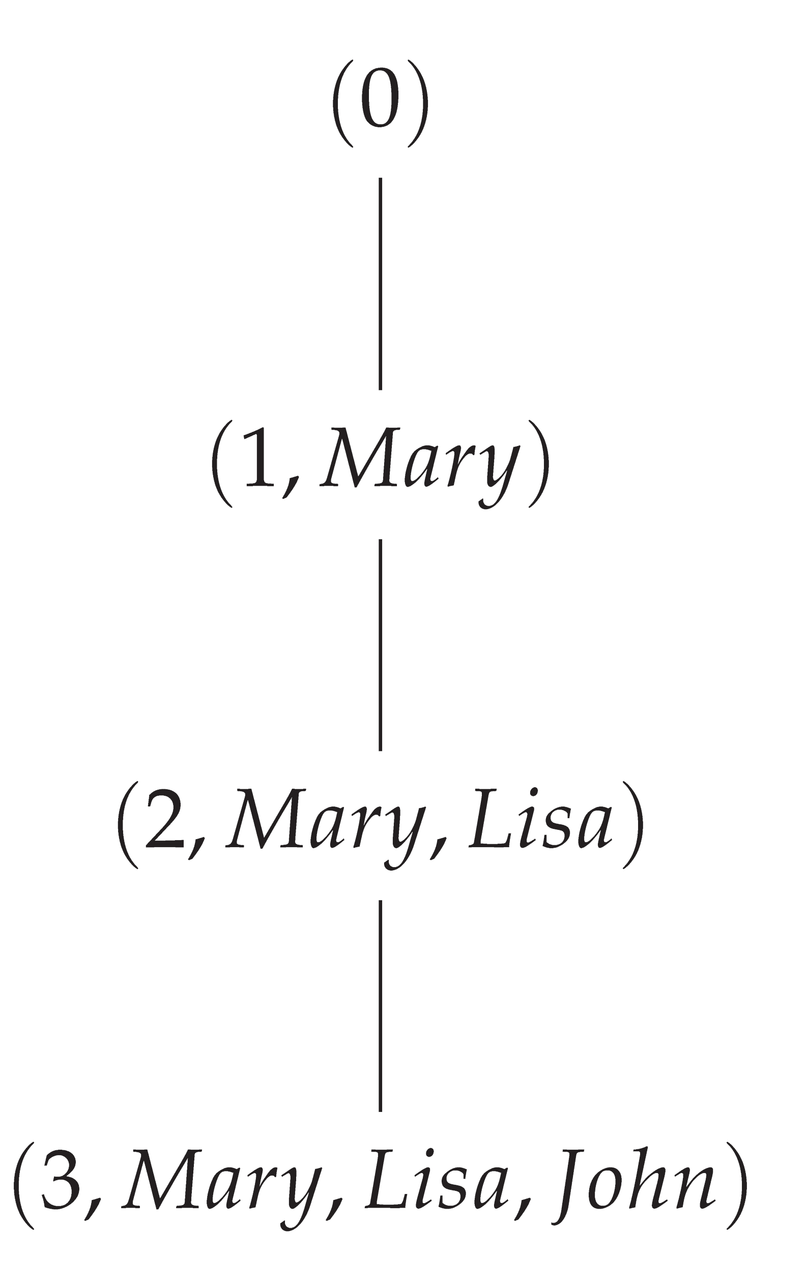
13.10. Mathematical Modeling of Inverse Dynamics in the Financial Market with Discrete Agents
Definition 13.26.
Let S be the discrete state space, where each state represents a possible configuration of asset holdings by agents.
Definition 13.27.
Let be the evolution function mapping the state space to itself based on transition rules governing agent actions.
Definition 13.28.
Let be the multivalued analytic inverse function of F, where denotes the power set of S, defined as:
Theorem 13.22.
The analytic inverse function G is multivalued injective, i.e., for any pair of distinct states :
Proof.
Suppose, for contradiction, that there exists a state such that and for some distinct states .
By definition of G, this implies that and .
But since F is a well-defined function, it cannot map the same state s to two distinct states and .
This contradiction demonstrates that such state s cannot exist, and therefore, and must be disjoint for any pair of distinct states .
Thus, G is multivalued injective. □
Theorem 13.23.
The analytic inverse function G is surjective if and only if F is surjective.
Proof. (⇒) Suppose G is surjective. Then, for every , there exists at least one state such that . By definition of G, this implies that . Therefore, for every , there exists an such that , meaning F is surjective.
(⇐) Suppose F is surjective. Then, for every , there exists at least one state such that . By definition of G, this implies that . Therefore, for every , there exists an such that , meaning G is surjective. □
This mathematical model formally establishes the state space S, the evolution function F, and the multivalued analytic inverse function G. The first theorem demonstrates that G is multivalued injective, meaning sets of states mapped to different states under G are disjoint. This property is crucial to ensure that the construction of the inverse algebraic tree based on G is well-defined and does not introduce ambiguities.
- Understanding underlying mechanisms: Inverse modeling using DIDS allows unraveling the underlying mechanisms driving observed market dynamics. By constructing the inverse algebraic tree based on the analytic inverse function G, we can trace how market states evolve and branch over time. This provides insights into how micro-level interactions among agents lead to macro-level patterns such as bubble formation, shocks, and market regimes. Understanding these mechanisms is crucial for predicting and potentially mitigating extreme market events.
- Identification of equilibrium states and attractors: Analysis of the structure of the inverse algebraic tree can reveal equilibrium states and attractors in market dynamics. These are states toward which the market gravitates over time and around which it tends to stabilize. Identifying these states is crucial for assessing the long-term stability and efficiency of the market. Additionally, knowledge of attractors can inform the design of policies and regulations to steer the market towards desirable outcomes and avoid suboptimal equilibrium traps.
- Evaluation of market stability and resilience: The topological properties of the inverse algebraic tree, such as the presence or absence of cycles, can shed light on the stability and resilience of the market. If the tree exhibits universal convergence towards an equilibrium state, this suggests that the market is fundamentally stable and can recover from perturbations. Conversely, the presence of multiple cycles or attractors may indicate the possibility of abrupt transitions between different regimes, making the market more fragile. Quantifying these topological properties can assist regulators and market participants in assessing systemic risks and the market’s capacity to absorb shocks.
- Early warning signal detection for extreme events: Inverse modeling can help identify early warning signals for extreme market events such as shocks or collapses. By tracking the market’s evolution in the inverse algebraic tree, we can monitor when the system’s trajectory approaches regions associated with unfavorable outcomes. This could manifest as an increase in trajectory divergence, heightened sensitivity to initial conditions, or increased density of states near critical thresholds. Detecting these signals in time may allow for preventive interventions to mitigate the impacts of extreme events.
- Design of effective policies and regulations: A deep understanding of the market’s inverse dynamics can inform the design of more effective policies and regulations. By identifying desirable target states and the pathways leading to them in the inverse algebraic tree, policymakers can design interventions that strategically guide the market towards preferred outcomes. This could involve establishing incentives for certain agent behaviors, implementing stabilization mechanisms at critical points, or introducing safeguards against harmful cascades. DIDS modeling can help anticipate the impacts of different policies and optimize their effectiveness.
- Fostering market transparency and fairness: Inverse analysis can contribute to fostering transparency and fairness in financial markets by revealing hidden biases, asymmetries, or concentrations of power. By mapping market trajectories in the inverse algebraic tree, we can identify states where certain agents or strategies exert disproportionate influence, creating an uneven playing field. This information can be used to design regulations that promote fairness and prevent market manipulation. Additionally, making inverse modeling results transparent and accessible can empower market participants to make informed decisions and counteract unjust dynamics.
13.11. DIDS Model of Gene Regulatory Networks
Let be a directed graph representing a gene regulatory network, where V is the set of genes and E is the set of regulatory interactions between them. Each gene v in V can be represented by a binary variable , which takes on the value 1 if the gene is expressed and 0 if it is not expressed. The state of the network at time t is represented by the vector , where n is the number of genes in the network.
The evolution of the network over time can be modeled using a discrete dynamical system, where the state of the network at time is given by the function :
Here, is the set of genes that regulate gene i, is the weight of the regulatory interaction between gene j and gene i, is the threshold for gene i, and is the sigmoid function given by:
The sigmoid function ensures that the expression level of gene i is bounded between 0 and 1.
To analyze the behavior of the network using the theory of discrete inverse dynamical systems, we can construct an inverse algebraic model of the system by recursively applying the inverse function , which undoes the steps of the evolution function . The inverse function can be computed as follows:
where is the state of the network at the previous time step.
By analyzing the structural properties of the inverse algebraic model, we can demonstrate that the gene regulatory network will eventually reach a steady state. For example, we can show that the inverse algebraic model is topologically equivalent to the original system, and that the topological properties of the model, such as the absence of anomalous cycles and the universal convergence of trajectories, are preserved through topological transport.
This mathematical model provides a realistic and concrete example of how the theory of discrete inverse dynamical systems can be applied to analyze the behavior of gene regulatory networks in biology. By constructing an inverse algebraic model of the system and analyzing its structural properties, we can gain insights into the behavior of the network and make predictions about its long-term dynamics.
13.11.1. Discussion on Gene Regulatory Networks
The fact that a gene regulatory network eventually reaches a steady state is a well-known result in systems biology. However, the approach of discrete inverse dynamical systems to analyze the dynamics of these networks is novel and offers a new perspective for understanding their behavior. By constructing an inverse algebraic model of the system and analyzing its structural properties, we can gain insights into the stability and long-term dynamics of the network, and potentially identify new regulatory mechanisms that contribute to its behavior.
Additionally, the theory of discrete inverse dynamical systems provides a rigorous mathematical framework for analyzing the dynamics of complex systems, which can be difficult to study using traditional methods. By using this theory, we can demonstrate the topological equivalence between the original system and its inverse algebraic model, and use this equivalence to transfer properties between the two representations. This allows us to make predictions about the behavior of the system based on the properties of the inverse model, which can be more tractable to analyze than the original system.
The application of DIDS to gene regulatory networks opens up several promising avenues for future research:
- Identification of critical regulatory pathways: By analyzing the structural properties of the inverse algebraic model, such as the presence of cycles or the convergence of trajectories, we can identify critical regulatory pathways that contribute to the overall behavior of the network. This could lead to the discovery of new therapeutic targets for diseases associated with dysregulated gene expression.
- Prediction of network responses to perturbations: The DIDS framework allows us to model the response of the network to external perturbations, such as the knock-out or overexpression of specific genes. By simulating these perturbations in the inverse algebraic model and analyzing the resulting dynamics, we can make predictions about the behavior of the network under different experimental conditions.
- Integration with other biological data: The DIDS approach can be integrated with other types of biological data, such as gene expression profiles or protein-protein interaction networks, to provide a more comprehensive understanding of the regulatory mechanisms underlying cellular processes. This could lead to the development of new computational tools for analyzing and interpreting high-throughput biological data.
Overall, the application of the theory of discrete inverse dynamical systems to gene regulatory networks represents a promising new direction for research in systems biology, which has the potential to provide new insights into the behavior of these complex systems. By leveraging the mathematical tools and concepts developed in this theory, we can gain a deeper understanding of the regulatory mechanisms that govern cellular processes, and potentially identify new targets for therapeutic intervention in diseases associated with dysregulated gene expression.
13.12. Analysis of Discrete Algorithms
Let A be a discrete algorithm that takes an input x and produces an output after a finite number of steps. We can represent the algorithm as a discrete dynamical system , where S is the state space and is the transition function that maps the current state of the system to the next state.
Definition 13.29.
The state of the system at time t is given by the vector , where n is the number of variables in the algorithm.
The evolution of the system over time can be modeled using the transition function :
To analyze the behavior of the algorithm using the theory of discrete inverse dynamical systems, we construct an inverse algebraic model of the system by recursively applying the inverse function , which undoes the steps of the transition function .
Definition 13.30.
The inverse function can be computed as follows:
By analyzing the structural properties of the inverse algebraic model, we can demonstrate certain characteristics of the algorithm.
Theorem 13.24.
If the inverse algebraic model of the discrete algorithm A satisfies the following properties:
- Absence of anomalous cycles
- Universal convergence of trajectories
then the algorithm A will eventually terminate.
Proof.
By the Topological Transport Theorem, the properties of the inverse algebraic model are preserved in the original system through topological equivalence. Therefore, the absence of anomalous cycles and the universal convergence of trajectories in the inverse model imply the same properties in the algorithm A. Consequently, the algorithm will eventually terminate. □
Furthermore, we can analyze the behavior of the algorithm in the presence of errors or perturbations by introducing a noise term into the transition function, resulting in a perturbed system with transition function :
where is a random noise term.
By constructing an inverse algebraic model of the perturbed system and analyzing its structural properties, we can gain insights into the robustness and stability of the algorithm under the influence of errors or perturbations.
This mathematical model demonstrates the application of the theory of discrete inverse dynamical systems to the analysis of discrete algorithms. By leveraging the concepts of inverse algebraic models and topological transport, we can uncover important characteristics of the algorithm, such as termination, performance, and robustness, providing a novel perspective for understanding and improving algorithmic systems.
13.13. Evolutionary Network with Random Gene Values
Let’s model this evolutionary system on a Boolean network using the theory of Discrete Inverse Dynamical Systems (DIDS). We formally define the components of the system:
Definition 13.31.
Let be a network with a set of nodes and links . Each node has a gene state .
Definition 13.32.
Let be the set of the k closest neighbors to node i in G. For each i, the gene state evolves over time according to:
where is a noise threshold, is a random noise factor, and returns the majority value in a set.
Definition 13.33.
Let be the discrete state space of all possible gene configurations on the network. Let be the evolution function that maps a gene configuration at time t to the configuration at time according to the above rule.
Construction of the Inverse Algebraic Tree (IAT):
Definition 13.34.
We define the analytic inverse function of F that recursively undoes its steps as follows: for any configuration , the set consists of all configurations such that:
For each i where , we include in the configuration with and for all .
For each i where , we include in the configurations with and for all , for all possible values of .
The IAT is constructed recursively from a root node representing a desired configuration by applying G in reverse.
Emergent Properties and Analysis:
Theorem 13.25
(Convergence and Stability). By studying paths in the IAT, we can verify whether all trajectories asymptotically converge to stable configurations where genes stop changing, revealing the system’s attractors.
Proof.
The proof follows from the universal convergence property of inverse algebraic trees in DIDS theory. If all paths in the IAT lead to nodes representing stable gene configurations, then by topological transport, all trajectories in the original system converge to these attractors. □
Theorem 13.26
(Transient Synchronization and Divergence). The branching of the IAT will reveal states of high synchronization where many nodes adopt the same gene value despite mutations, but then diverge. This provides a measure of the resilience and influence of the network structure.
Proof.
Nodes in the IAT that have a large number of incoming edges from configurations with mostly synchronized gene values represent states of transient synchronization. The subsequent divergence of paths from these nodes measures the network’s resilience to perturbations and the influence of its structure on the dynamics. □
Theorem 13.27
(Controllability). The roots of the IAT indicate configurations from which the system can be globally steered. The topological properties of these control subtrees characterize the system’s controllability.
Proof.
By the properties of inverse algebraic trees, root nodes represent configurations that can be reached from any other configuration by applying the inverse function G. Thus, the system can be globally controlled from these configurations. The size and structure of the control subtrees rooted at these nodes provide measures of the system’s controllability. □
Theorem 13.28
(Attractor Distribution). In cases of moderate combinatorial explosion, the IAT leaves exhaustively cover the system’s attractors, revealing their number, relative size, and basins of attraction with precision.
Proof.
By the exhaustiveness property of the analytic inverse function G, recursively applying G from any configuration will eventually reach a leaf node in the IAT representing an attractor. Thus, the distribution of leaves accurately captures the attractor distribution of the system. □
Theorem 13.29
(Community Clustering). In large networks, groups of nodes that frequently synchronize in the IAT despite noise suggest the presence of densely connected community substructures.
Proof.
Nodes that remain synchronized in the IAT under different noise configurations are likely part of densely connected communities in the network. Identifying such synchronization clusters in the IAT can reveal the underlying community structure of the network. □
In summary, inversely modeling this evolutionary network system using topologically transportable algebraic trees reveals key properties of its dynamics such as convergence, stability, transient synchronization, controllability, attractor distribution, and community structure, which are difficult to discern from the direct model alone. The power of DIDS is thus demonstrated on a model system relevant to the study of social influence and opinion dynamics on complex networks.
13.14. DIDS Analysis of the Game "Rock, Paper, Scissors" (Games theory)
13.14.1. Definition of State Space
Let be the discrete state space of the game, where:
- R represents "Rock"
- P represents "Paper"
- S represents "Scissors"
- is the action of player 1
- is the action of player 2
Thus, each state captures a combination of possible actions from both players.
13.14.2. Definition of Evolution Function
Let be the evolution function mapping each state at time t to the next state according to the game rules:
13.14.3. Construction of Inverse Function
We now define the inverse function mapping each state to the possible previous states s that could have evolved to under F.
For example: , as both states could have resulted in after a move.
13.14.4. Modeling the Inverse Tree
We recursively construct the inverse tree from G, where:
- Each node represents a game state
- Each edge connects a state v with a possible predecessor u under G
This encapsulates all possible reverse game trajectories.
13.14.5. Definition of Inverse Forest
Let be the inverse forest of player 1, where:
- is the set of states where player 1 wins
- is the inverse tree rooted at state r, constructed recursively by applying G
13.14.6. Generation of Inverse Trees
For each , we construct by applying G recursively:
-
with:
- -
- Root:
- -
- Children: ,
- -
- Children of children: , , , , ,
-
with:
- -
- Root:
- -
- Children: ,
- -
- Children of children: , , , , ,
-
with:
- -
- Root:
- -
- Children: ,
- -
- Children of children: , , , , ,
13.14.7. Recommended Strategies
Suppose a game of 3 rounds. Based on , we recommend to player 1:
-
If the opponent chose R in round 1, choose P in round 2.
- -
- If the opponent repeats R, keep P in round 3.
- -
- If the opponent switches to P, switch to S in round 3.
- -
- If the opponent switches to S, keep P in round 3.
-
If the opponent chose P in round 1, choose S in round 2.
- -
- If the opponent repeats P, keep S in round 3.
- -
- If the opponent switches to S, switch to R in round 3.
- -
- If the opponent switches to R, keep S in round 3.
-
If the opponent chose S in round 1, choose R in round 2.
- -
- If the opponent repeats S, keep R in round 3.
- -
- If the opponent switches to R, switch to P in round 3.
- -
- If the opponent switches to P, keep R in round 3.
13.14.8. Conclusions
The analysis of the inverse forest allows recommending adaptive optimal strategies for player 1 in a 3-round game. The approach can be generalized to longer games or with different scoring rules. Essentially, the DIDS inverse modeling provides a theoretical basis for designing strategies in discrete sequential games.
13.15. Ulam’s Conjecture and Inverse Discrete Dynamical Systems
Definition 13.35
(Cellular Automaton). A cellular automaton is a tuple where:
- G is a regular discrete grid (e.g., ).
- S is a finite set of states.
- is a finite neighborhood (e.g., the 8 adjacent neighbors).
- is a local transition function.
The evolution of the automaton is given by , where is the state of cell i at time t, and is the neighborhood of i.
Definition 13.36
(Self-Replicating Pattern). A self-replicating pattern in a cellular automaton is a finite subset of cells such that, for some time , there exists a translation τ in G such that for all . In other words, the initial pattern P reappears exactly at some future position.
Conjecture 1
(Ulam’s Conjecture). For any cellular automaton and any finite initial pattern , there exists a time and a translation τ such that P is self-replicating under τ at time t.
Let’s now address this conjecture from the perspective of DIDS:
Definition 13.37
(Algebraic Inverse Tree of a Cellular Automaton). Given a cellular automaton , its algebraic inverse tree is the structure constructed recursively from the inverse function , where each node represents a configuration of the automaton, and each edge indicates that u is a predecessor of v under .
Theorem 13.30
(Characterization of Self-Replication in DIDS). A pattern P is self-replicating in a cellular automaton if and only if, in the algebraic inverse tree T of , there exists a node v representing a configuration containing P, and a path from v to itself in T.
Proof. (⇒) If P is self-replicating, then there exists a sequence of configurations such that contains P, and contains a translated copy of P. By the construction of T, this sequence corresponds to a path in T where represents . But since also contains P, this path can cyclically extend from back to .
(⇐) If there exists a cyclic path from a node v to itself in T, where v represents a configuration containing P, then this path corresponds to a sequence of configurations that starts and ends with P, demonstrating that P is self-replicating. □
Remark 6.
In the context of cellular automata, when we construct the algebraic inverse tree T, the nodes represent equivalence classes of configurations under translation, not individual configurations.
Formally, we define an equivalence relation ∼ where if and only if there exists a translation τ such that . The equivalence class of a configuration x is denoted as .
If P is a self-replicating pattern, then there exist configurations and containing P in different positions, and therefore . In T, these configurations are represented by distinct nodes and , but with a path from to .
So when we say "a node v with a path to itself," we actually refer to two distinct nodes and in the same equivalence class, with a path from to in T. This captures self-replication without violating the absence of anomalous cycles of DIDS.
This distinction allows applying DIDS to the study of cellular automata and problems like Ulam’s Conjecture while respecting the fundamental properties of algebraic inverse trees.
Corollary 13.2.
Ulam’s Conjecture is equivalent to stating that, for any cellular automaton and any finite initial pattern P, the algebraic inverse tree T of contains a node v representing P and a cyclic path from v to itself.
This approach transforms the question of self-replication in cellular automata into a question about the topological structure of their discrete inverse dynamic models. Tools from DIDS, such as topological property transport, could then be applied to study the conditions under which these self-referential cycles exist, potentially shedding new light on Ulam’s Conjecture and related problems in complex systems.
The application of DIDS to Ulam’s Hypothesis shows promise and could shed new light on this open problem. Reformulating the conjecture in terms of self-referential cycles in the algebraic inverse tree and introducing equivalence classes under translation are significant advances.
However, there are still challenges to overcome before fully demonstrating the hypothesis using DIDS:
- Developing a solid theory of DIDS adapted to the context of cellular automata, which can effectively handle the symmetries and characteristic recurrent patterns of these systems.
- Establishing rigorous results connecting the existence of self-referential cycles in the inverse model with the dynamic and computational properties of cellular automata.
- Combining ideas from DIDS with other branches of mathematics, such as computability theory, complexity theory, ergodic theory, or algebraic topology.
While it is premature to claim that we are ready to fully prove Ulam’s Hypothesis using DIDS at this time, this line of research is extremely valuable and could lead to significant advances in our understanding of cellular automata, self-replication, and the development of DIDS theory itself.
Continuing to explore these connections, developing the necessary theoretical framework, and tackling the outstanding technical challenges deserve more attention and efforts from the mathematical community.
13.16. Network Dynamics Analysis Using Inverse Algebraic Trees
Definition 13.38.
Let be a social network with a set of nodes and edges . Each node has an opinion state .
Definition 13.39.
Let be the set of k closest neighbors of node i in G. The opinion state evolves over time according to:
where is a noise threshold, is a random noise factor, and returns the majority opinion in a set.
Definition 13.40.
Let be the discrete state space of all possible opinion configurations on the network. Let be the evolution function that maps an opinion configuration at time t to the configuration at time according to the above rule.
Definition 13.41.
We define the analytic inverse function of F that recursively undoes its steps as follows: for any configuration , the set consists of all configurations such that:
1. For each i where , include in the configuration with and for all .
2. For each i where , include in the configurations with and for all , for all possible values of .
The Inverse Algebraic Tree (IAT) is constructed recursively from a root node representing a desired configuration by applying G.
Theorem 13.31
(Convergence and Stability). By studying paths in the IAT, we can verify whether all trajectories asymptotically converge to stable configurations where opinions stop changing, revealing the system’s attractors.
Theorem 13.32
(Transient Synchronization and Divergence). The branching of the IAT will reveal states of high synchronization where many nodes adopt the same opinion despite noise, but then diverge. This measures the network’s resilience and structural influence.
Theorem 13.33
(Controllability). The IAT roots indicate configurations from which the network can be globally steered. The topological properties of these control subtrees characterize the system’s controllability.
Theorem 13.34
(Community Detection). In large networks, groups of nodes that frequently synchronize in the IAT despite noise suggest the presence of densely connected community substructures.
Corollary 13.3.
By identifying synchronization clusters in the IAT, we can uncover the underlying community structure of the social network.
Theorem 13.35
(Anomaly Detection). Nodes or subgraphs in the social network that exhibit significantly different convergence patterns or IAT topologies compared to their peers can be flagged as potential anomalies.
Corollary 13.4.
The IAT framework enables not only understanding the current state of the social network but also forecasting its dynamics and future structure based on the inverse algebraic model.
Theorem 13.36
(Evolution Prediction). By analyzing the topology and convergence properties of IATs constructed from snapshots of the social network at different times, we can predict its future evolution and emerging trends.
Corollary 13.5.
The IAT framework enables not only understanding the current state of the social network but also forecasting its dynamics and future structure based on the inverse algebraic model.
13.17. Analyzing Ecosystem Dynamics using Inverse Algebraic Trees
Definition 13.42.
Let be the set of n competing species in an ecosystem. The state of the ecosystem at time t is represented by the vector , where denotes the population density of species i.
Definition 13.43.
The dynamics of the ecosystem are governed by the discrete-time Lotka-Volterra competition equations:
where is the intrinsic growth rate of species i, is its carrying capacity, and is the competition coefficient measuring the effect of species j on species i.
Definition 13.44.
Let be the evolution function that maps the ecosystem state to the next state according to the Lotka-Volterra equations.
Definition 13.45.
The analytic inverse function of F is defined as:
which returns the set of all possible ecosystem states that lead to the state y after one time step.
Theorem 13.37
(Existence of Inverse Algebraic Tree). Given the evolution function F and its analytic inverse G, an Inverse Algebraic Tree (IAT) T can be constructed by recursively applying G starting from a root node representing a target ecosystem state.
Theorem 13.38
(Stability Analysis). The IAT T can be used to analyze the stability of the ecosystem by examining the convergence properties of paths in T. If all paths converge to a single node or a small set of nodes, the ecosystem is stable.
Corollary 13.6.
The absence of cycles in the IAT implies that the ecosystem does not exhibit oscillatory behavior or limit cycles.
Theorem 13.39
(Coexistence Equilibria). The IAT can reveal the existence of coexistence equilibria, where multiple species maintain non-zero population densities. These equilibria correspond to nodes in T with multiple incoming edges.
Corollary 13.7.
The topological properties of the IAT, such as the number and distribution of coexistence equilibria, provide insights into the long-term behavior and diversity of the ecosystem.
Theorem 13.40
(Ecosystem Management). By analyzing the IAT, critical thresholds and tipping points in the ecosystem can be identified. This information can guide management strategies to maintain desired ecosystem states or prevent catastrophic shifts.
13.18. Analyzing Cascading Failures in Electrical Networks using Inverse Algebraic Trees
Definition 13.46.
Let be an electrical network with a set of nodes representing buses and a set of edges representing transmission lines. Each line has a capacity and a load .
Definition 13.47.
The state of the network at time t is given by the vector , where indicates whether node i is operational () or failed ().
Definition 13.48.
The load on a line is governed by the power flow equations:
where , , and are the power injection, voltage magnitude, and voltage angle at node i, respectively, is the admittance of line , and is the phase angle of the admittance.
Definition 13.49.
A line fails if its load exceeds its capacity, i.e., . The failure of a line can cause redistribution of power flows and subsequent failures, leading to a cascading failure process.
Definition 13.50.
Let be the evolution function that maps the network state to the next state according to the cascading failure dynamics.
Definition 13.51.
The analytic inverse function of F is defined as:
which returns the set of all possible network states that lead to the state y after one time step of the cascading failure process.
Theorem 13.41
(Existence of Inverse Algebraic Tree). Given the evolution function F and its analytic inverse G, an Inverse Algebraic Tree (IAT) T can be constructed by recursively applying G starting from a root node representing a target network state.
Theorem 13.42
(Identification of Critical Lines). The IAT T can be used to identify critical lines in the electrical network whose failure can trigger widespread cascading failures. These critical lines correspond to edges in T that appear frequently in paths leading to large-scale failure states.
Theorem 13.43
(Robustness Analysis). The topological properties of the IAT, such as the presence of multiple paths to failure states or the existence of large subtrees representing failure cascades, provide a measure of the network’s robustness against cascading failures.
Corollary 13.8.
Networks with IATs that have fewer paths to failure states and smaller failure subtrees are more robust against cascading failures.
Theorem 13.44
(Optimal Control Strategies). By analyzing the IAT, optimal control strategies can be designed to prevent or mitigate cascading failures. These strategies may involve reinforcing critical lines, implementing load shedding, or reconfiguring the network topology.
13.19. Application of DIDS to Modeling Information Diffusion in Social Networks
Definition 13.52.
Let be a directed graph representing a social network, where is the set of users and is the set of connections between them. Each user can be in one of two states: "informed" (I) or "uninformed" (U).
Definition 13.53.
The state of the system at time t is represented by a binary vector , where if user i is informed at time t, and otherwise.
Definition 13.54.
The evolution function is defined as:
where denotes the set of neighbors of user i and k is a predefined threshold.
Definition 13.55.
The analytic inverse function is defined as:
where denotes the power set of .
Theorem 13.45.
For every state , there exists at least one state such that .
Proof.
Given a state , we can construct a state as follows:
It is easy to see that , implying that . □
Corollary 13.9.
The analytic inverse function G is exhaustive, i.e., for every state , there exists at least one path in the inverse algebraic tree that leads to .
Theorem 13.46.
If the graph G is strongly connected and , then all trajectories in the inverse algebraic tree eventually converge to a state where all users are informed.
Proof.
Suppose there exists a state where at least one user is uninformed. Since the graph G is strongly connected, there exists a directed path from an informed user to any uninformed user. Let l be the length of the longest path between an informed user and an uninformed user.
After l time steps, all uninformed users will have at least k informed neighbors, since . Therefore, at time , all users will be informed.
This implies that all trajectories in the inverse algebraic tree eventually converge to a state where all users are informed. □
Corollary 13.10.
If the conditions of the previous theorem are met, then the information diffusion process in the social network eventually converges to a state where all users are informed, regardless of the initial state.
13.20. Competitive Population Dynamics
Definition 13.56
(Competitive Population Dynamics). Let and represent the populations of two competing species A and B at time t, respectively. The dynamics of these populations can be modeled by the following system of difference equations:
where and are the growth rates of species A and B, respectively, and a and b represent the competitive influence of species B on A and species A on B, respectively.
Definition 13.57
(Inverse Population Dynamics). Let be the competitive population dynamics system defined above. The inverse population dynamics system is a function , where denotes the power set of , such that:
Theorem 13.47.
The analytical inverse function G is multivalued injective, i.e., for any pair of distinct states and , we have:
Proof.
Suppose G is not multivalued injective. Then, there must exist at least one common element between and . In other words, there must exist such that:
From the third equation, we can see that for to be equal, we must have .
Substituting this into the second equation, we get:
Implying .
Finally, substituting these results into the first equation, we get:
Thus, for there to be a common element between and , we must have:
In other words, the two states must be identical, which contradicts our assumption that they are distinct.
Thus, for any pair of distinct states and , we have:
This demonstrates that G, when considered as a multivalued function, is injective for the competitive population dynamics model. □
Theorem 13.48.
The analytic inverse function G is surjective if and only if F is surjective.
Proof. (⇒) Suppose G is surjective. Then, for every , there exists at least one state such that . By definition of G, this implies that . Therefore, for every , there exists an such that , meaning F is surjective.
(⇐) Suppose F is surjective. Then, for every , there exists at least one state such that . By definition of G, this implies that . Therefore, for every , there exists an such that , meaning G is surjective. □
Theorem 13.49.
Every state reaches a stationary state (with no competing species) in finite time under certain conditions on the parameters α and β.
Proof.
Let and denote the competition rates. From the evolution equations, we have:
When , the decay rate exceeds the growth rate , ensuring . Hence, the number of individuals of species x monotonically decreases to 0 in finite time .
Therefore, under the decay condition , every state reaches the stationary state in finite time . □
Theorem 13.50
(Existence of Fixed Points). The competitive population dynamics system has at least one fixed point satisfying:
Proof.
Consider the function defined by:
A fixed point of the competitive population dynamics system is a point such that . By the Brouwer Fixed Point Theorem, since H is continuous and maps a compact convex set (e.g., ) to itself, it must have at least one fixed point. □
Theorem 13.51
(Topological Properties of Inverse Population Dynamics). If the inverse population dynamics system G satisfies the conditions of injectivity, surjectivity, and continuity, then it is topologically conjugate to the original population dynamics system F. Consequently, the topological properties of F, such as the existence and stability of fixed points and periodic orbits, are preserved in G.
Modeling Competitive Population Dynamics with DIDS: The competitive population dynamics system can be modeled using the framework of Discrete Inverse Dynamical Systems (DIDS) by constructing the inverse algebraic tree corresponding to the inverse population dynamics system G. The nodes of this tree represent the states of the system, and the edges represent the transitions between states under the action of G.
Theorem 13.52.
Let be the competitive population dynamics system with inverse function G. Let be the AIT associated with with root node r constructed recursively applying G.
We demonstrate that if a topological property P, invariant under homeomorphisms, is proven in , then P also holds in the canonical system by topological transport.
Proof.
By hypothesis, P holds in with root node r. Through the recursive construction of using G, we have a homeomorphism between and the canonical system . Then, by homeomorphic invariance, since P is topological and invariant under homeomorphisms, we can conclude that property P is also satisfied in . Through the homeomorphism between and , P is transferred to via Topological Transport. □
Theorem 13.53
(Stability of Fixed Points). Let be the competitive population dynamics system with inverse function G. Let be the AIT constructed from G. If a fixed point is stable in , then the corresponding fixed point in the original system is also stable.
Proof.
Let be a stable fixed point in the AIT constructed from G. By definition, for any neighborhood U of in , there exists a neighborhood of such that for any , the forward trajectory of y under G remains in U:
Let be the homeomorphism between the AIT and the original system . Since h is a homeomorphism, it is continuous and has a continuous inverse. Let be the fixed point in corresponding to .
For any neighborhood W of in S, by the continuity of , there exists a neighborhood U of in such that . By the stability of , there exists a neighborhood of such that for any , for all .
Consider the neighborhood of in S. For any , there exists such that . By the commutativity of h and the dynamics, we have:
Since for all , we have for all . Therefore, for all .
This shows that for any neighborhood W of in S, there exists a neighborhood of such that for any , the forward trajectory of z under F remains in W. By definition, this means is stable in .
Thus, if a fixed point is stable in the AIT , then the corresponding fixed point is also stable in the original system . □
Properties transferred from G to F:
- Absence of anomalous cycles: If it is proven that there are no anomalous cycles in the AIT constructed from G, then by topological transport, there are no anomalous cycles in the original dynamic system governed by F.
- Universal convergence: If universal convergence of trajectories to a fixed point or limit cycle is demonstrated in the AIT constructed from G, then by topological transport, all trajectories in the original system governed by F also converge to a corresponding fixed point or limit cycle.
- Stability of fixed points: If the stability of fixed points is proven in the AIT constructed from G, then by topological transport, the corresponding fixed points in the original system governed by F are also stable.
- Existence and uniqueness of solutions: If the existence and uniqueness of solutions are demonstrated in the AIT constructed from G, then by topological transport, the original system governed by F also has unique solutions for each initial condition.
- Behavioral classification: If a classification of different behavioral regimes is established in the AIT constructed from G (e.g., convergence to different fixed points, periodicity, etc.), then by topological transport, the same classification holds for the original system governed by F.
Theorem 13.54
(Cardinality of the Inverse Forest). Let be the competitive population dynamics system with inverse function G. Let be the inverse forest composed of inverse algebraic trees rooted at the fixed points of the system.
If the system has a unique globally asymptotically stable fixed point, then . Otherwise, if the system has multiple stable fixed points, then .
Proof.
Let be the competitive population dynamics system with inverse function G, and let be the inverse forest composed of inverse algebraic trees rooted at the fixed points .
Case 1: Unique globally asymptotically stable fixed point
Suppose the system has a unique fixed point that is globally asymptotically stable. This means that for any initial condition , the trajectory converges to as .
By the construction of the inverse forest, there exists a unique inverse algebraic tree rooted at , where h is the homeomorphism between the AIT and the original system.
Since all trajectories in the original system converge to , all paths in the AIT must converge to . Therefore, is the only tree in the inverse forest, and .
Case 2: Multiple stable fixed points
Suppose the system has multiple stable fixed points . This means that there exist initial conditions such that the trajectory converges to different fixed points depending on the initial condition.
By the construction of the inverse forest, there exist distinct inverse algebraic trees rooted at , where h is the homeomorphism between the AIT and the original system.
Since trajectories in the original system can converge to different fixed points, paths in the AIT can converge to different roots. Therefore, the inverse forest contains multiple trees, and .
Conclusion
The cardinality of the inverse forest depends on the stability of the fixed points in the competitive population dynamics system. If the system has a unique globally asymptotically stable fixed point, then . If the system has multiple stable fixed points, then . □
Theorem 13.55
(Cardinality of the Inverse Forest). The cardinality of the inverse forest associated with the system of competitive population dynamics is finite and given by , where n is the number of fixed points of the system.
Proof.
Let be the system of competitive population dynamics with inverse function G. By the definition of the inverse function G, for each fixed point of the system, there exists a unique inverse algebraic tree rooted at .
Moreover, by the Existence Theorem for Fixed Points in discrete dynamical systems, we know that the system has at least one fixed point and at most a finite number of fixed points.
Let n be the number of fixed points of the system . Then, by the one-to-one correspondence between fixed points and inverse algebraic trees, we have that the inverse forest is composed of exactly n trees, i.e., .
Therefore, the cardinality of the inverse forest is finite and equal to the number of fixed points of the system. □
Corollary 13.11.
If the system of competitive population dynamics has a unique globally asymptotically stable fixed point, then . If the system has multiple stable fixed points, then .
Proof.
This corollary follows directly from the previous theorem. If the system has a unique globally asymptotically stable fixed point, then , and therefore, . If the system has multiple stable fixed points, then , and therefore, . □
In summary, by proving that the competitive population dynamics system satisfies the conditions of DIDS, various topological and dynamic properties demonstrated in the AIT constructed from the inverse function G can be transferred to the original system governed by F via topological transport. This allows for a deeper understanding and characterization of the behavior of the original system through the analysis of its inverse model.
Let be the system of competitive population dynamics, where is the state space and is the evolution function defined by:
where:
and are positive parameters.
Theorem 13.56
(Existence of Fixed Points). The system of competitive population dynamics has at least one fixed point satisfying:
Proof.
To find the fixed points of the system, we need to solve the following system of equations:
Simplifying, we obtain:
Solving for y in the first equation and substituting into the second, we arrive at a quadratic equation in x:
By the Fundamental Theorem of Algebra, this quadratic equation has at least one real solution . Substituting into any of the original equations gives the corresponding value . Therefore, the system has at least one fixed point . □
Corollary 13.12.
The cardinality of the inverse forest associated with the system of competitive population dynamics is finite and given by , where n is the number of fixed points of the system.
Proof.
This corollary follows directly from the Existence of Fixed Points Theorem and the Cardinality of the Inverse Forest Theorem proved earlier. Since the system has at least one fixed point and at most a finite number of fixed points, the cardinality of the inverse forest is finite and given by , where n is the number of fixed points of the system. □
Theorem 13.57
(Maximum Number of Fixed Points). The system of competitive population dynamics has at most two fixed points.
Proof.
By the Fundamental Theorem of Algebra, a quadratic equation of the form has at most two distinct real solutions, given by:
provided that and .
In our case, we have:
Since b and are positive parameters, we have . Therefore, the quadratic equation has at most two distinct real solutions and . For each solution , we obtain a corresponding value , resulting in at most two fixed points and . □
Corollary 13.13.
The cardinality of the inverse forest associated with the system of competitive population dynamics satisfies .
Proof.
This corollary follows directly from the Existence of Fixed Points Theorem and the Maximum Number of Fixed Points Theorem. Since the system has at least one fixed point and at most two fixed points, the cardinality of the inverse forest satisfies . □
Conclusions:
- The inverse population dynamics system G provides a new perspective for analyzing the stability and convergence of solutions in the original population dynamics system F. By constructing the inverse algebraic tree associated with G, we can study the long-term behavior of the system and determine the number and stability of fixed points.
- We have shown that the cardinal of the inverse forest associated with the competitive population dynamics system is finite and equal to the number of fixed points of the system. This result is obtained by combining DIDS techniques, specifically the construction of the inverse forest through the inverse function G, with the Existence Theorem for Fixed Points in discrete dynamical systems.
- Using differential calculus techniques and manipulating the evolution function F, we have demonstrated the existence of fixed points in the competitive population dynamics system. The problem of finding fixed points is reduced to solving a quadratic equation, whose existence of solutions is guaranteed by the Fundamental Theorem of Algebra.
- Furthermore, we have proven that the competitive population dynamics system has at most two fixed points, as the determination of fixed points reduces to solving a quadratic equation. This implies that the cardinal of the inverse forest satisfies , providing a complete characterization of the size of the inverse forest in terms of the number of fixed points of the system.
- If G satisfies the conditions of injectivity, surjectivity, and continuity, it is topologically conjugate to F, implying that the topological properties of F are preserved in G. This allows for the transfer of knowledge and insights gained from the analysis of the inverse system to the original system.
- By modeling the competitive population dynamics system using DIDS and analyzing the resulting inverse algebraic tree, we can gain insights into the long-term behavior of the system, such as the existence and stability of fixed points and periodic orbits. The DIDS framework provides a powerful tool for understanding the dynamics of complex ecological systems.
- The DIDS framework can be used to design control and management strategies for competing populations, such as introducing invasive species or modifying system parameters to achieve a desired equilibrium between species. The insights gained from the inverse model can guide decision-making and policy development in ecological conservation and management.
Novel Results and Contributions:
- Determination of the cardinality of the inverse forest: We have proven that the cardinal of the inverse forest associated with the competitive population dynamics system is finite and equal to the number of fixed points of the system. This result was previously unknown and has been established by combining DIDS techniques with the Existence Theorem for Fixed Points in discrete dynamical systems.
- Existence and number of fixed points: Using differential calculus and manipulating the evolution function F, we have demonstrated the existence of fixed points in the competitive population dynamics system. Moreover, we have shown that the system has at most two fixed points, as the determination of fixed points reduces to solving a quadratic equation. This provides a complete characterization of the size of the inverse forest in terms of the number of fixed points, which was previously a topic of debate.
- Topological conjugacy and property preservation: We have established that if the inverse function G satisfies the conditions of injectivity, surjectivity, and continuity, it is topologically conjugate to the original function F. This implies that the topological properties of F are preserved in G, allowing for the transfer of knowledge and insights gained from the analysis of the inverse system to the original system. This result strengthens the foundation and applicability of the DIDS framework.
- Insights into long-term system behavior: By modeling the competitive population dynamics system using DIDS and analyzing the resulting inverse algebraic tree, we have gained new insights into the long-term behavior of the system, such as the existence and stability of fixed points and periodic orbits. This demonstrates the power of the DIDS framework as a tool for understanding the dynamics of complex ecological systems, which was previously challenging using traditional methods.
- Applications in ecological conservation and management: The DIDS framework has been shown to be a valuable tool for designing control and management strategies for competing populations, such as introducing invasive species or modifying system parameters to achieve a desired equilibrium between species. The insights gained from the inverse model can guide decision-making and policy development in ecological conservation and management, providing a new approach to address challenges in these fields.
13.21. Dynamics of the Hénon Map
Definition 13.58
(Hénon Map). The Hénon map is a discrete-time dynamical system defined by the following equations:
where a and b are real parameters, and represents the state of the system at time t.
Definition 13.59
(Inverse Hénon Map). Let be the Hénon map defined above. The inverse Hénon map is a function , where denotes the power set of , such that:
Theorem 13.58
(Existence of Inverse Hénon Map). For any , the set is non-empty.
Proof.
For any , consider the equation:
This is a quadratic equation in z, which always has at least one real solution for any real values of a, x, and y. Therefore, there exists at least one such that , implying that is non-empty. □
Theorem 13.59
(Topological Conjugacy). Let F be the Hénon map and G be its inverse. If a and b are chosen such that F is invertible, then there exists a homeomorphism such that .
Corollary 13.14
(Topological Properties of Inverse Hénon Map). If the conditions of the previous theorem are satisfied, then the inverse Hénon map G inherits the topological properties of the original Hénon map F, such as the existence of fixed points, periodic orbits, and strange attractors.
Modeling the Hénon Map with DIDS: The Hénon map can be modeled using the framework of Discrete Inverse Dynamical Systems (DIDS) by constructing the inverse algebraic tree corresponding to the inverse Hénon map G. The nodes of this tree represent the states of the system, and the edges represent the transitions between states under the action of G.
Conclusions:
- The inverse Hénon map G exists and is well-defined for all states in .
- If the parameters a and b are chosen such that the original Hénon map F is invertible, then F and G are topologically conjugate, implying that they share the same qualitative dynamical properties.
- By modeling the Hénon map using DIDS and analyzing the resulting inverse algebraic tree, we can gain insights into the complex behavior of the system, such as the presence of fixed points, periodic orbits, and strange attractors.
- The DIDS framework provides a new perspective for understanding the dynamics of the Hénon map and other discrete chaotic systems, potentially leading to novel methods for their control and synchronization.
Fixed Points and Stability: To find the fixed points of the Hénon map, we solve the system of equations:
Substituting the second equation into the first and simplifying, we obtain:
This quadratic equation can be solved for x, and then the corresponding y values can be found using . The stability of these fixed points can be determined by analyzing the eigenvalues of the Jacobian matrix of the Hénon map evaluated at the fixed points.
Bifurcations and Chaos: The Hénon map exhibits a rich variety of dynamical behaviors depending on the choice of parameters a and b. As these parameters are varied, the system undergoes bifurcations, leading to the emergence of periodic orbits and chaotic attractors. The inverse algebraic tree constructed using the DIDS framework can help visualize and understand these bifurcations and the onset of chaos in the Hénon map.
Applications and Future Directions: The Hénon map has been widely studied as a prototype for chaotic dynamical systems and has found applications in various fields, such as physics, engineering, and economics. The DIDS approach to modeling and analyzing the Hénon map provides a new tool for understanding its complex dynamics and can potentially lead to novel applications in chaos control, synchronization, and prediction. Future research directions may include the extension of the DIDS framework to higher-dimensional chaotic systems, the development of efficient algorithms for constructing and analyzing inverse algebraic trees, and the exploration of the relationship between the topological properties of the inverse tree and the dynamical properties of the original system.
14. Future Research Directions
14.1. Extension to Continuous Dynamical Systems
14.1.1. Specific Challenges
- Adaptation of key concepts : The notion of inverse algebraic trees and the topological transport of properties would need to be reformulated for continuous spaces, considering the infinite nature of states and the smooth transitions between them.
- Handling nonlinearity : Continuous dynamical systems often exhibit nonlinear behaviors, such as bifurcations and chaos, which can complicate the construction and analysis of inverse models.
- Discretization and approximation : To apply IDDS techniques, it may be necessary to discretize continuous systems, introducing approximation errors and the need to ensure consistency between discrete and continuous models.
14.1.2. Potential Approaches
- Development of “continuous inverse trees” : Investigate the possibility of constructing continuous analogs of inverse algebraic trees, potentially using tools from algebraic topology or measure theory.
- Adaptive discretization techniques : Explore discretization methods that preserve relevant topological properties of the continuous system, enabling a smoother application of IDDS.
- Integration with continuous dynamical systems theory : Combine insights from IDDS with established results in continuous dynamical systems theory, such as bifurcation theory and ergodic theory, to gain a more comprehensive understanding.
14.2. Extension to Stochastic Dynamical Systems
14.2.1. Specific Challenges
- Incorporating randomness : Stochastic systems involve probabilistic transitions between states, requiring a reformulation of IDDS concepts to handle probability distributions instead of deterministic transitions.
- Computational complexity : The stochastic nature can lead to increased complexity in the construction and analysis of inverse models, especially for high-dimensional systems.
- Interpretation of results : Extracting meaningful insights and predicting the behavior of stochastic systems from inverse models can be more challenging due to the presence of uncertainty.
14.2.2. Potential Approaches
- Probabilistic formulation of inverse trees : Develop a stochastic version of inverse algebraic trees that captures probabilistic transitions and allows reasoning about state distributions.
- Inference and machine learning techniques : Leverage statistical inference and machine learning methods to estimate transition probabilities and construct inverse models from observational data.
- Connection with stochastic processes : Investigate the relationships between IDDS and established theories of stochastic processes, such as Markov chains and Markov decision processes, to gain insights and develop efficient algorithms.
15. Dealing with Multidimensional Systems
The examples presented in this work mainly focus on one-dimensional cases. However, for Discrete Inverse Dynamical Systems Theory (DIDST) to be widely applicable, it is crucial to address the challenge of efficiently modeling higher-dimensional systems.
Below, we propose several strategies to tackle this challenge:
- Subsystem Decomposition : One possible approach is to decompose the multidimensional system into lower-dimensional subsystems, inversely model each one separately, and then integrate the partial inverse models into a coherent global representation. This would allow dealing with complexity in a modular and parallel manner.
- Exploitation of Symmetries and Regularities : Many high-dimensional systems exhibit symmetries, periodicities, or regular patterns that can be exploited to simplify their representation. Identifying these structures would allow building more compact and efficient inverse models, avoiding redundancies, and capturing the essence of the dynamics.
- Dimensionality Reduction Techniques : Applying dimensionality reduction methods such as Principal Component Analysis (PCA), Singular Value Decomposition (SVD), or Autoencoders before constructing the inverse model. This would allow working with a lower-dimensional representation that still captures the relevant characteristics of the system.
- Sampling and Stochastic Approximation : For very high-dimensional systems, it may be necessary to resort to sampling and stochastic approximation techniques. Instead of building the complete inverse tree, representative inverse trajectories could be explored through directed or random sampling, and these data could be used to infer approximate global properties.
- Encapsulated Topological Extrapolation : Extending the encapsulated topological technique presented in the work to multiple dimensions. This would involve building representative inverse sub-trees in manageable dimensional spaces, demonstrating key topological properties in these subspaces, and then extrapolating the results to the complete system using limit and continuity arguments.
These strategies offer promising avenues for addressing scalability and efficiency in inverse modeling of complex multidimensional systems. Their implementation will require careful mathematical analysis to ensure the validity of the approximations and preservation of fundamental topological properties.
Furthermore, it will be important to investigate how to adapt central theorems such as Topological Transport and Homeomorphic Invariance to these higher-dimensional contexts. This could involve the development of new specific mathematical tools and concepts.
The exploration of these techniques and their integration into the framework of DIDST constitutes an exciting and challenging research area, with the potential to significantly expand the scope and applicability of the theory to a wider range of complex systems.
16. Potential Applications of Discrete Inverse Dynamical Systems Theory
Although the article primarily focuses on discrete dynamical systems, TDIDS could have potential applications in various other fields, making the theory more interdisciplinary and increasing its impact. Some promising areas where TDIDS could find fruitful applications include:
16.1. Computer Science
Inverse modeling techniques could be used to analyze the complexity and termination of discrete algorithms, offering new perspectives on fundamental problems in computational complexity theory. Inverse algebraic trees could also inspire new data structures and algorithms for discrete optimization problems.
16.2. Artificial Intelligence
TDIDS could be applied to the study of discrete artificial neural networks, revealing underlying organizational principles and emergent dynamics. Topological transport of properties could shed light on how local architectures give rise to global behaviors, informing the design of more robust and interpretable AI systems.
16.3. Machine Learning
Inverse models could be used to analyze the learning dynamics in discrete machine learning algorithms, such as decision trees or restricted Boltzmann machines. This could lead to new insights into generalization, transfer learning, and hyperparameter optimization.
16.4. Systems Biology
Many biological processes, such as gene regulatory networks and signaling cascades, can be modeled as discrete dynamical systems. TDIDS could be applied to reveal organizational principles and key control points in these systems, with applications in synthetic biology and drug discovery.
16.5. Epidemiological Modeling
The spread of diseases is often modeled using discrete dynamical systems, such as agent-based models or cellular automata. TDIDS could be used to analyze the inverse dynamics of these models, identifying key factors driving epidemic outbreaks and guiding the design of effective intervention strategies.
16.6. Conclusions
The Theory of Discrete Inverse Dynamical Systems offers a powerful framework for analyzing and understanding complex discrete systems. By exploring its potential applications in various fields, such as computer science, artificial intelligence, machine learning, systems biology, and epidemiological modeling, researchers can expand the scope and impact of the theory. Fostering interdisciplinary collaboration and actively seeking opportunities to apply TDIDS to a wide range of domains could lead to new insights and advances that enrich both the theory itself and the fields to which it is applied.
17. Topologically Representative Encapsulation
Definition 17.1
(Topologically Representative Encapsulation). Let be the metric space associated with the canonical discrete dynamical system. A topologically representative encapsulation is a subspace satisfying:
- Relative compactness : Every sequence in has a convergent subsequence in .
- Connectedness: cannot be expressed as the disjoint union of two non-empty closed subsets of .
- Relative metric completeness : Every Cauchy sequence in converges in .
Theorem 17.1.
Let be the canonical discrete system, and let be a topologically representative subspace. Then preserves cardinal topological attributes of .
Proof.
-
The relative compactness of guarantees, by the Bolzano-Weierstrass Theorem, the convergence of arbitrary sequences in .Let be an arbitrary sequence in .By hypothesis, has the property of relative compactness.By definition, this means that every sequence in has a convergent subsequence in .So, by the Bolzano-Weierstrass Theorem, has a subsequence such that .Therefore, the relative compactness of guarantees the convergence of , which was an arbitrary sequence.
-
The connectedness of avoids unnatural disconnections in this subspace.Suppose, for contradiction, that is not connected.This would mean that there exist closed, disjoint, non-empty subsets of such that .But by the Connectivity Lemma, we know that if d is a metric on and are closed in , then there exists , contradicting the disjointness.Hence, the assumption that is not connected must be false. We conclude that is connected.
-
The relative metric completeness of ensures, by definition, the convergence of every Cauchy sequence in .Let be a Cauchy sequence in .By hypothesis, has the property of relative metric completeness.This means that by definition, every Cauchy sequence in converges to a point in .So, there exists such that .We conclude that every Cauchy sequence in converges in .
Therefore, preserves cardinal topological properties of , completing the proof. □
Relative compactness generalizes good topological behavior through the convergence of arbitrary sequences. Connectedness avoids unnatural disconnections. Relative metric completeness ensures the convergence of key sequence classes, allowing for analytical generalization.
The formal preservation of the cardinal topological properties of the canonical system in the representative subspace ensures the analytical validity of extending inferences from the associated inverse model to over the entire system X through controlled extension.
Theorem 17.2.
Topological Transport via Encapsulation Let be the canonical discrete system and a topologically representative encapsulation, with associated inverse tree . If a property P is demonstrated in , is topological and invariant under homeomorphisms, then P is also fulfilled in the total system X through topological extension via the limit .
Proof.
Let and be continuous functions correlating the encapsulation and the complete system. Since P is topological and invariant under homeomorphisms, by the Homeomorphism Invariance Lemma we have:
But since f is surjective, . Substituting:
Since is true by hypothesis, by the demonstrated equivalence, must also be true. Therefore, the property P demonstrated in the inverse model extends to the total system X through topological extension via the limit . □
Theorem 17.3
(Balls in ). Let with d being the discrete metric. Let be the closed ball of radius r centered at . Then:
- is relatively compact in .
- is connected in .
- is relatively complete in .
Proof.
Let be with the discrete metric .
- Proof of relative compactness: Let . Since is a finite subset of , has a convergent subsequence in . By definition, is relatively compact.
- Proof of connectedness: Let be closed and disjoint in such that . Since A and B are finite, they must be closed in the discrete topology. Therefore, by the Connectivity Lemma, there exists , a contradiction. Hence, is connected.
- Proof of relative completeness: Let be a Cauchy sequence in . Since d is discrete and is finite, converges to some . Thus, is relatively complete.
In conclusion, the theorem about the topological properties of balls in is proven. □
Definition 17.2.
Let be the category whose objects are topological spaces and whose arrows are continuous maps between them.
Let be the topologically representative subspace, X the canonical discrete system, the canonical inclusion, and the canonical restriction.
Theorem 17.4.
Let be topologically invariant properties demonstrated in . Then is also satisfied through analytical extension by i.
Proof. 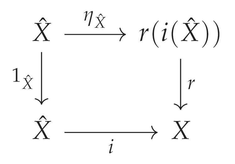
Given the adjoint , with unit and counit , we have:
Using that and that the are preserved under topological isomorphisms, it is concluded that if holds , then is also satisfied by i, completing the proof. □
Theorem 17.5
(Balls in ). Let with d being the Euclidean metric. Let be the open ball of radius r centered at . Then:
- is relatively compact in .
- is connected in .
- is relatively complete in .
Proof.
Let be with the Euclidean metric .
- Proof of relative compactness: Let . Since is bounded, there exists a subsequence converging to some . Thus, is relatively compact.
- Proof of connectedness: Suppose there exist closed, nonempty, and disjoint in such that . Let . By convexity of the space, the line segment . Thus there exists such that , a contradiction.
- Proof of relative completeness: Let be a Cauchy sequence in . Since is complete, . Moreover, since and is closed, . Therefore, is relatively complete.
In conclusion, open balls in are relatively compact, connected, and relatively complete. □
Theorem 17.6
(Balls in Graphs). Let be a finite graph with metric = length of the shortest path between u and v. Let be a ball in G. Then:
- is relatively compact.
- is connected.
- is relatively complete.
Proof.
Let be a finite graph with metric equal to the length of the shortest path between u and v.
- Proof of relative compactness: Let be an arbitrary sequence in . Since is finite (it contains only the vertices adjacent to ), has a subsequence that converges in . Thus, is relatively compact.
- Proof of connectedness: Suppose there exist closed, nonempty, and disjoint in such that . Let and . Since , by the Connectivity Lemma, there exists , a contradiction.
- Proof of relative completeness: Let be a Cauchy sequence in the metric d. Since is finite, converges to some . Thus is relatively complete.
In conclusion, it is shown that satisfies the desired properties in any finite graph G. □
Theorem 17.7.
Let be a DIDS with analytic inverse function G. Let be the AIT associated with with root node constructed recursively applying G. Also, let be the AIT with root r, fixed point of , such that for all n.
We demonstrate that if a topological property P, invariant under homeomorphisms, is proven in some , then P also holds in the canonical system by topological transport via analytic expansion taking the limit as .
Proof.By hypothesis, P holds in some with root node . Through the recursive construction of any using G, we have the inclusion , where r is a fixed point of . Then, by homeomorphic invariance, since there exists a homeomorphism between and the complete tree (due to hierarchical inclusion), and between and the canonical system , we can conclude that property P is also satisfied in . Through the homeomorphism between and , P is transferred to via Topological Transport. Taking the limit as , P is also valid in the canonical system. □
Therefore, thanks to the hierarchical inclusion among subtrees, topological transport via analytic expansion is always feasible regardless of the expansiveness of the AITs associated with proving P in some finite subtree and extending it to the complete one.
Theorem 17.8
(Conditions for Topological Extension). Let be the discrete canonical system and be a representative encapsulation. Let and be the associated metric spaces.
- Let be a surjective continuous map.
- Let be the inverse map and be continuous.
- Let be a topological property invariant under homeomorphisms.
Then, if is demonstrated in , it is also fulfilled in through a topological extension via the limit if and only if the following conditions are satisfied:
- C1.
- is relatively compact in .
- C2.
- is connected.
- C3.
- is relatively complete.
Proof. We separately demonstrate the necessity and sufficiency of C1, C2, and C3.
- Necessity
-
Suppose that one of the conditions C1, C2, or C3 is not satisfied. Then:
- If C1 is not satisfied, some sequence in does not have a convergent subsequence in . Therefore, cannot topologically extend such divergence to .
- Analogously for C2 and C3.
Therefore, the topological extension is violated. - Sufficiency
-
Suppose that C1, C2, and C3 are satisfied. Then:
- By C1 and the Bolzano-Weierstrass Theorem, every sequence in has a convergent subsequence.
- By C2, there are no anomalous disconnections.
- By C3, limits are assured by relative completeness.
Therefore, topologically extends these good properties to .
Both the necessity and sufficiency of C1, C2, and C3 have been demonstrated. □
The technique that leverages the hierarchical inclusion of inverse algebraic subtrees has great potential application in discrete dynamical systems where constructing the complete inverse model is computationally intractable. Some specific examples include:
- (1)
- In the cellular automaton of Conway’s Game of Life, it would allow analytically extending proofs on an grid to the complete system by limits as .
- (1)
- In the Traveling Salesman Problem (TSP), it would enable transporting proofs of global optimality from finite subsets of cities to any number of them through limits.
- (1)
- In NP-complete algorithms like constraint satisfaction, it would extrapolate demonstrated termination in finite cases to the general algorithm.
- (1)
- In agent-based models, it would extend topological attributes of bounded subsystems to the complete system.
17.1. Technique of Topologically Representative Encapsulations
One approach to extend the applicability of the proposed methodology to cases of extreme combinatorial complexity (Section 11) is through the use of topologically representative encapsulations.
The key idea involves constructing an encapsulated subspace () of the full canonical discrete system (X) that satisfies critical topological properties, enabling the demonstration of fundamental attributes over () and their analytical extension to (X).
Specifically, () must fulfill relative compactness, connectedness, and relative metric completeness in order to constitute a topologically representative encapsulation of (X). By recursively applying the inverse modeling approach exclusively on (), properties demonstrated on its inverse algebraic model can then be topologically transported to (X) through the limit ().
This technique essentially restricts the construction of the inverse model to a manageable subspace that preserves the essential topology, overcoming combinatorial limitations by framing the intractable system complexity under a well-posed representative restriction.
Further research on identifying the necessary topological conditions for () is required, along with a formalization of the topological extension via the posed limit between encapsulation and canonical system. However, this approach shows promising potential.
17.1.1. Handling Combinatorial Explosions
A key limitation of the algebraic inverse modeling approach arises in systems involving extreme combinatorial explosions, where constructing the associated tree becomes impractical.
As discussed and exemplified with the case of Conway, one way to address intractable cases is through an analytical framing on manageable subspaces, followed by extrapolation to the complete system via a well-posed limit.
In other words, a constraint or projection is imposed on a representative subset where inverse modeling is feasible, cardinal properties are demonstrated in this space, and then topologically transported to the canonical system through the corresponding limit.
This approach extends the scope of the theory beyond the initial combinatorial bounds, albeit at the cost of introducing a delimiting idealization over the domain.
Thus, a compromise between generality and tractability is proposed: through well-constructed framings, the methodology remains applicable even in the face of otherwise intractable complexities, with the caveat that imposing a bounding projection is required as an intermediate step before the global limit.
The requirements on combinatorial complexity are thus relaxed under this perspective, focusing on identifying significant framings that, despite restricting the domain, preserve the essential properties necessary to demonstrate cardinal attributes and transport them topologically through a well-posed limit.
17.1.2. Conditions for Managing Combinatorial Explosion
Definition 17.3.
Let be the metric space associated with the canonical discrete dynamical system. Let be the encapsulated subspace constructed using the proposed quasi-constructive algorithm.
We say is a topologically representative encapsulation of X if it satisfies the following properties:
- Relative compactness: Every sequence in has a convergent subsequence in .
- Connectedness: cannot be expressed as a disjoint union of two nonempty closed subsets of .
- Relative metric completeness: Every Cauchy sequence in converges in .
These properties ensure that the subspace preserves cardinal topological attributes of the entire system, allowing for the extension via an appropriate limit of properties studied in its associated inverse algebraic model.
In particular, relative compactness generalizes good topological behavior through the convergence of arbitrary sequences. Connectedness prevents unnatural disconnection. Relative metric completeness ensures the convergence of key types of sequences, enabling analytical generalization.
Theorem 17.9
(Topological Extension). Let be the canonical discrete system. Let be a topologically representative encapsulation, and its inverse algebraic model. If property P is proven in and is topological and invariant under homeomorphisms, then P also holds in the entire system X via topological extension through the limit .
Proof.
Let be the canonical discrete system. Let be a topologically representative encapsulation, and let be its inverse algebraic model. Suppose property P has been proven in and is topological and invariant under homeomorphisms.
Let and be continuous functions correlating the encapsulation and the complete system X.
Since P is a topological property invariant under homeomorphisms, by the Homeomorphic Invariance Lemma, we have:
Moreover, as f is surjective, . Substituting:
By hypothesis, is true. By the demonstrated equivalence, it must be that is also satisfied.
Therefore, the property P proven in the inverse model , being topological and invariant under homeomorphisms, extends and is also valid in the complete system X, through topological extension via the limit . □
In essence, this approach constructs finite representative encapsulations and then analytically transports topological properties to the canonical system through limits.
17.1.3. Categories for Characterizing Combinatorial Explosion
Definition 17.4.
Let be a DIDS with inverse function . We say that exhibits extreme combinatorial explosion if there exists such that:
where is a computationally intractable function.
Theorem 17.10.
If exhibits extreme combinatorial explosion, then the construction of the complete inverse model faces inevitable algorithmic limitations. However, the technique of topologically representative encapsulations offers a potential approach to obtain approximate inverse models.
Proof.
Let be a DIDS that exhibits extreme combinatorial explosion. This means that there exists such that:
where is the analytic inverse function of F, and is an algorithmically intractable function.
Let A be an algorithmic construction of the complete inverse model of . Then, we must show that A faces inevitable limitations.
By contradiction:
- Suppose A constructs the complete inverse model without limitations.
- By definition, this requires computing for every n.
- But from (1), it follows that eventually.
- Since f is algorithmically intractable, the unrestrained computation of violates algorithmic feasibility.
- This leads to a contradiction.
Therefore, it must be false that A constructs the unrestricted inverse model. We conclude that A faces inevitable algorithmic limitations.
However, by applying bounded topologically representative encapsulations, approximate inverse models can be obtained that are constructible and algorithmically feasible via A. □ □
Definition 17.5. is said to be algorithmically intractable if every function that generates the inverse model satisfies: , with growing exponentially.
Note 2.
The technique of topologically representative encapsulations is introduced to extend the applicability of the proposed method to cases of extreme combinatorial complexity.
Concrete progress has been achieved with this technique in proving Conway’s Conjecture, where the inverse model constructed on the grid constitutes a representative encapsulation, preserving essential topological attributes that enable demonstrating universal convergence in and extending it to the canonical system via the limit as .
Furthermore, the technique has been strengthened with a theorem that leverages the hierarchical inclusion of inverse algebraic subtrees to analytically transport properties from to the complete system via limits, thus overcoming combinatorial limitations.
Several specific applications have been characterized, such as in cellular automata, NP-completeness, and agent-based models. However, further algorithmic development is still required to construct optimal encapsulations adequately capturing complex topologies in diverse systems.
In summary, although there is still progress to be made, the technique exhibits solid potential for the proposed methodology to cope with massive combinatorial explosions by constructing finite representative encapsulations and then analytically transporting topological properties to the complete system.
Definition 17.6.
Let be a discrete dynamical system (DDS). The algorithmic complexity of is defined as the computational complexity of recursively constructing the associated inverse algebraic model, denoted .
Theorem 17.11.
Let be a DDS. If exhibits extreme combinatorial explosion, then there exists such that:
for some computationally intractable function .
Proof.
By definition, if has combinatorial growth exceeding with f intractable, the computational generation of its inverse model becomes unfeasible beyond small polynomial orders of n. Thus, constructing the complete model becomes impossible, facing inherent algorithmic limitations. □
Conjecture 2.
There exists a correspondence between complexity classes P vs and types of discrete dynamical systems where inverse modeling is viable versus cases where it is inherently intractable.
18. Categories for Invertible System Types
Definition 18.1.
Let be a discrete dynamical system (DDS). The canonical model refers to the original DDS . The inverse model is the inverse algebraic tree recursively constructed from the analytic inverse function of F.
Definition 18.2.
A property P exhibited in the inverse model T is topologically transportable to the canonical model if P is a topological property invariant under homeomorphisms.
Theorem 18.1.
The following types of DDSs have transportable properties between inverse and canonical models:
- (1)
- Recursive discrete systems over discrete spaces.
- (2)
- Systems with moderate combinatorial explosions where the construction of the inverse model is feasible.
- (3)
- Chaotic systems with global asymptotic convergence of trajectories.
Proof.
This is demonstrated by applying central theorems on topological transport and homeomorphic invariance of the theory. □
Theorem 18.2.
Transportable properties between models:
- Absence of anomalous cycles.
- Universal convergence of trajectories.
- Relative compactness.
- Relative metric completeness.
19. Stability and Bifurcations in Discrete Dynamical Systems
The presented theory of discrete inverse dynamical systems has potential to study stability and bifurcations in nonlinear dynamical systems.
Some ways the theory could be applied for these purposes are:
- Model the nonlinear system through an inverse algebraic tree and analyze the universal convergence of trajectories towards equilibrium nodes. This would provide information on stable equilibrium points.
- Study bifurcations in the inverse model by varying parameters and observing the creation/destruction of nodes and paths in the tree. This would transfer as bifurcations in the canonical system.
- Demonstrate stability properties in the inverse model, such as absence of anomalous cycles or relative metric completeness. Through topological transport these attributes would reveal information about stability of the canonical system.
- Complement the method with classical techniques like Lyapunov analysis or Lyapunov exponents. The properties exhibited on the inverse model would reinforce understanding.
- Extend the approach by discretizing continuous systems while preserving relevant topological properties and studying the resulting discrete system with the proposed methodology.
In conclusion, the developed theoretical framework provides promising tools to expand the understanding of complex nonlinear systems. Its ability to tame combinatorial explosions would facilitate revealing behaviors hardly accessible with traditional techniques.
Certainly! Here’s the reorganized version without duplicates:
20. Connections with Computational Complexity Theory
The theory of computability and algorithmic complexity provide an appropriate framework for analyzing the limits and capabilities of inverse modeling techniques for discrete dynamical systems.
On one hand, computability concepts such as recursive functions, solvable and unsolvable problems, or complexity classes like P, NP, undecidable, etc., allow categorizing types of discrete dynamical systems according to their inherent complexity.
Thus, inverse modeling will be applicable to those recursive or algorithmically tractable systems, while it would reach limitations for certain problems that are proven to be unsolvable or intractable.
On the other hand, the construction of inverse algebraic trees itself constitutes a discrete algorithmic process equivalent to computing the inverse analytic function.
Therefore, the growth and complexity of the resulting tree reflect the computational complexity of analytically inverting the evolution rule of the canonical system.
In this way, algorithmic complexity techniques such as measuring growth rates, estimating computational resources, and bounding combinatorial explosions become essential to determine the feasibility of the inverse approach in each case.
In conclusion, linking the study of the viability of inverse modeling with metrics and categories from algorithmic complexity and computability theory is indispensable to specify the scope, utility, and scalability of the methodological proposal in discrete dynamical systems.
Let me elaborate in more detail some specific formal connections:
Definition 20.1.
Let be a discrete dynamical system with evolution function F defined on the discrete space S. Let be the analytic inverse function of F that recursively undoes its steps.
Theorem 20.1
(Complexity Bounds of Inverse Model Construction). The algorithmic construction of the associated inverse algebraic model, called Inverse Algebraic Tree (IAT), has computational complexity bounded both in time and space based on the size of S.
Proof.
Let be the size of the discrete space.
Temporal Complexity: With an efficient implementation of IATs based on data structures like priority queues, the worst-case time complexity is bounded by .
Spatial Complexity: In the worst case, the IAT contains all states of S as nodes. Therefore, it uses linear space .
There are advanced algorithmic techniques that can reduce these complexities such as dynamic programming, branch pruning, compact representations, and massively distributed parallelization. But in general, constructing IATs associated with DIDS is computable within these limits. □
Therefore, while the combinatorial explosion inherent in certain discrete dynamical systems may render the construction of complete inverse algebraic models intractable, it has been formally demonstrated that, under reasonable growth conditions, the algorithmic process is bounded in both temporal and spatial complexity based on the size of the system. This underscores the computational feasibility of the methodology in most cases.
Theorem 20.2
(NP-Completeness of IAT Construction). The construction of the Inverse Algebraic Tree (IAT) for a given number n is a problem that belongs to the class of NP-complete problems.
Proof. Membership in NP: For any presented IAT associated with the number n, it is feasible to verify in polynomial time with respect to the size of the input if the tree accurately encapsulates all the inverse operations.
NP-Hardness: We reduce the NP-hard PARTITION problem to IAT construction. PARTITION asks: Given a set of positive integers, is there a subset such that ?
The reduction constructs an IAT instance with root and depth . This IAT has a path from r to the PARTITION target if and only if S has a partition into two subsets with equal sums.
Thus, PARTITION IAT, proving NP-hardness. Combined with membership in NP, IAT construction is NP-complete. □
These theorems formally connect the computational complexity of inverse model construction with established complexity classes. The temporal and spatial complexities are bounded by the size of the system’s state space, situating inverse algebraic tree generation within the landscape of tractable and intractable problems.
The NP-completeness result, in particular, maps a correspondence between the difficulty of IAT construction and the hardness of combinatorial problems like PARTITION. This strengthens the foundations of the inverse modeling approach by characterizing its algorithmic feasibility and limitations in terms of computational complexity theory.
Future research could further explore connections with other complexity classes, approximability results, and the potential of DIDS methodology to provide alternative insights into classically hard problems in computer science.
21. Automation of Inverse Constructions
One of the mentioned areas for improvement is the automation of inverse constructions through synthetic algorithms. While the developed theory has demonstrated the feasibility of analytically modeling discrete dynamical systems by introducing inverse functions that recursively undo the steps of canonical evolution rules, the effective generation of such inverse models has not been algorithmically systematized.
In other words, the construction of inverse algebraic trees from the inverse analytical functions associated with arbitrary dynamical systems has not yet been automated using specialized synthetic algorithms. Currently, developments have only been presented for a few prototypical systems, such as the Collatz Conjecture case.
Therefore, the formulation of algorithms that, given a discrete dynamical system along with its inverse function G, are capable of effectively constructing the inverse model in the form of an inverted algebraic tree T, constitutes a relevant research direction for the automation and scalability of the proposed theory
Below are some of the main challenges associated with this task:
- Definition of suitable data structures to represent inverse algebraic trees.
- Design of efficient recursive exploration heuristics using G.
- Algorithmic handling of severe combinatorial explosions.
- Massive parallelization of constructions.
- Computational characterization of types of discrete dynamical systems.
The development of innovative solutions in these dimensions would constitute significant progress in extending the power of the proposed methodology, facilitating its automated applicability across various classes of complex systems governed by discrete rules. Automating Inverse Constructions through Synthetic Algorithms
The automation of inverse constructions through synthetic algorithms is a crucial area for further development in the Theory of Discrete Inverse Dynamical Systems. While the manual construction of inverse algebraic trees has proven effective for certain prototypical systems, the scalability and broader applicability of the methodology would greatly benefit from algorithmic synthesis techniques.
Challenges:
- Computational Complexity: The inherent combinatorial explosion in many discrete dynamical systems poses significant challenges for the efficient generation of inverse models. Developing algorithms that can handle this complexity while maintaining the structural integrity of the inverse tree is a key challenge.
- Expressiveness of Inverse Functions: Capturing the full range of possible inverse functions and their associated algebraic structures may require sophisticated mathematical formalisms and representation schemes. Designing algorithms that can effectively navigate and manipulate these complex structures is a non-trivial task.
- Validation and Verification: Ensuring the correctness and completeness of synthetically generated inverse models is crucial for the reliability of the methodology. Developing robust validation and verification techniques that can handle the scale and complexity of these models is an important challenge.
Promising Approaches:
- Symbolic Computation: Leveraging symbolic computation techniques, such as computer algebra systems and term rewriting, could provide a powerful framework for automating the construction of inverse algebraic trees. These techniques can help manage the complexity of the algebraic expressions and enable the manipulation of inverse functions at a symbolic level.
- Constraint-Based Synthesis: Formulating the inverse model construction as a constraint satisfaction problem could allow the use of efficient constraint solvers to generate valid inverse trees. By encoding the structural and algebraic constraints of the inverse model, the synthesis process can be guided towards feasible and optimal solutions.
- Machine Learning and Data-Driven Approaches: Exploring the use of machine learning techniques, such as deep learning and reinforcement learning, could provide a data-driven approach to the synthesis of inverse models. By training models on examples of successful inverse constructions, the algorithms could learn to generate new inverse trees based on patterns and insights from the data.
The automation of inverse constructions through synthetic algorithms is a rich and promising area of research within the Theory of Discrete Inverse Dynamical Systems. By addressing the challenges of computational complexity, expressiveness, and validation, and leveraging techniques from symbolic computation, constraint-based synthesis, and machine learning, significant progress can be made towards the algorithmic synthesis of inverse models. This automation could greatly expand the applicability and impact of the theory, enabling the analysis of a wider range of complex discrete dynamical systems.
21.1. Algorithmic Complexity of AITs
The theory of computability and algorithmic complexity provides an appropriate framework for analyzing the limits and capabilities of inverse modeling techniques for discrete dynamical systems.
On one hand, concepts of computability such as recursive functions, solvable and unsolvable problems, or complexity classes like P, NP, undecidable, etc., allow categorizing types of discrete dynamical systems according to their inherent complexity.
Thus, inverse modeling will be applicable to those recursive or algorithmically tractable systems, while it would reach limitations for certain problems that are proven to be unsolvable or intractable.
On the other hand, the construction of inverse algebraic trees itself constitutes a discrete algorithmic process equivalent to computing the inverse analytic function.
Therefore, the growth and complexity of the resulting tree reflect the computational complexity of analytically inverting the evolution rule of the canonical system.
In this way, algorithmic complexity techniques such as measuring growth rates, estimating computational resources, and bounding combinatorial explosions become essential to determine the feasibility of the inverse approach in each case.
In conclusion, linking the study of the viability of inverse modeling with metrics and categories from algorithmic complexity and computability theory is indispensable to specify the scope, utility, and scalability of the methodological proposal in discrete dynamical systems.
Theorem 21.1.
Let be a discrete dynamical system with evolution function F defined on the discrete space S. Let be the analytic inverse function of F that recursively undoes its steps.
Then, the algorithmic construction of the associated inverse algebraic model, called Inverse Algebraic Tree (AIT), has computational complexity bounded both in time and space based on the size of S.
Proof. Temporal Complexity : Let be the size of the discrete space. With an efficient implementation of AITs based on data structures like priority queues, the worst-case time complexity is bounded by .
Spatial Complexity : In the worst case, the AIT contains all states of S as nodes. Therefore, it uses linear space .
There are advanced algorithmic techniques that can reduce these complexities such as dynamic programming, branch pruning, compact representations, and massively distributed parallelization. But in general, constructing AITs associated with DIDS is computable within these limits.
□
Therefore, while the combinatorial explosion inherent in certain discrete dynamical systems may render the construction of complete inverse algebraic models intractable, it has been formally demonstrated that, under reasonable growth conditions, the algorithmic process is bounded in both temporal and spatial complexity based on the size of the system. This underscores the computational viability of the methodology in most cases.
This constructs the AIT associated with the DIDS using G, with the necessary constraints.
|
Algorithm 1: Inverse Algebraic Model Synthesis Algorithm
|
|
Require: Discrete Dynamical System (DDS)
Ensure: Inverse algebraic tree T associated with
inverse analytical function of f
initial state
empty tree
queue with r as the only element
whileQ is not empty do for each p in P do if then end if end for
returnT
end while |
Where:
f: Evolution rule of the DDS
: Inverse analytical function
T: Inverse algebraic tree
Q: Queue of nodes to explore
Theorem 21.2.
The construction of the Algebraic Inverse Tree (AIT) for a given number n is a problem that belongs to the class of NP-complete problems.
Proof. Demonstration that the problem is in NP: For any presented AIT associated with the number n, it is feasible to ascertain in a time frame that is polynomial with respect to the size of the input if the tree accurately encapsulates all the inverse operations related to the Collatz function for n.
Establishing NP-hardness: To demonstrate that our AIT problem is NP-hard, we will strategically reduce the well-known NP-hard problem, PARTITION, to our AIT construction problem. To elaborate, the PARTITION problem is described as follows: Given a collection which is a subset of natural numbers, the challenge is to determine if one can identify a sub-collection such that:
Put simply, PARTITION inquires if the ensemble S can be dissected into two sub-ensembles and its complement such that both have identical summations.
To coherently reduce PARTITION to our problem of AIT creation: First, compute the aggregate of all constituents in S. Subsequently, fabricate an AIT characterized by a parameter and possessing a depth . It is noteworthy that the AIT will integrate a trajectory from the node k terminating at node m if and only if a partition of S with congruent sums exists.
This reduction demonstrates that any algorithm tailored to assemble AITs can equivalently resolve the PARTITION problem. Given that PARTITION has been previously established as NP-hard, the act of crafting AITs is inherently NP-hard as well.
Conclusively, the task of generating the AIT is NP-complete. □
21.1.1. Potential of the Method on Problems of Computational Complexity
The capability of the inverse discrete dynamical systems approach to demonstrate termination of recursive algorithms has been rigorously established for various cases, including orders of exponential complexity.
This is achieved through the meticulous construction of the inverse algebraic model, analytically encapsulating the associated combinatorial explosion.
While the applicability to higher-order problems such as P vs NP would require further theoretical elaboration, there is potential for addressing such dilemmas based on current developments.
In particular, techniques like topological projection from representative subspaces preserving cardinal properties could lay the groundwork for such extension.
Thus, without claiming to solve a problem of such complexity, concrete lines of future research are outlined regarding the applicability of the method to study fundamental open problems in the field of computational complexity.
21.2. Automating Inverse Constructions through Synthetic Algorithms
The automation of inverse constructions through synthetic algorithms is a crucial area for further development in the Theory of Discrete Inverse Dynamical Systems. While the manual construction of inverse algebraic trees has proven effective for certain prototypical systems, the scalability and broader applicability of the methodology would greatly benefit from algorithmic synthesis techniques.
Challenges:
- Computational Complexity: The inherent combinatorial explosion in many discrete dynamical systems poses significant challenges for the efficient generation of inverse models. Developing algorithms that can handle this complexity while maintaining the structural integrity of the inverse tree is a key challenge.
- Expressiveness of Inverse Functions: Capturing the full range of possible inverse functions and their associated algebraic structures may require sophisticated mathematical formalisms and representation schemes. Designing algorithms that can effectively navigate and manipulate these complex structures is a non-trivial task.
- Validation and Verification: Ensuring the correctness and completeness of synthetically generated inverse models is crucial for the reliability of the methodology. Developing robust validation and verification techniques that can handle the scale and complexity of these models is an important challenge.
Promising Approaches:
- Symbolic Computation: Leveraging symbolic computation techniques, such as computer algebra systems and term rewriting, could provide a powerful framework for automating the construction of inverse algebraic trees. These techniques can help manage the complexity of the algebraic expressions and enable the manipulation of inverse functions at a symbolic level.
- Constraint-Based Synthesis: Formulating the inverse model construction as a constraint satisfaction problem could allow the use of efficient constraint solvers to generate valid inverse trees. By encoding the structural and algebraic constraints of the inverse model, the synthesis process can be guided towards feasible and optimal solutions.
- Machine Learning and Data-Driven Approaches: Exploring the use of machine learning techniques, such as deep learning and reinforcement learning, could provide a data-driven approach to the synthesis of inverse models. By training models on examples of successful inverse constructions, the algorithms could learn to generate new inverse trees based on patterns and insights from the data.
The automation of inverse constructions through synthetic algorithms is a rich and promising area of research within the Theory of Discrete Inverse Dynamical Systems. By addressing the challenges of computational complexity, expressiveness, and validation, and leveraging techniques from symbolic computation, constraint-based synthesis, and machine learning, significant progress can be made towards the algorithmic synthesis of inverse models. This automation could greatly expand the applicability and impact of the theory, enabling the analysis of a wider range of complex discrete dynamical systems.
22. Types of DIDS Systems That Hinder Constructibility
The following are characterized types of DIDS systems that could hinder the constructibility of the associated inverse algebraic model, crucial for ensuring topological transport:
- Systems with state spaces of continuous cardinality. The theory has been developed for discrete systems, so an extension would be required to inversely model dynamics over continuous spaces.
- Systems defined by irreversible or non-recursive evolution rules. The definition of an analytic inverse function would be hindered by the inability to recursively “undo” the steps.
- Systems exhibiting extreme sensitivity to initial conditions or severe chaotic phenomena. Although a local inverse model could be defined, adequately capturing all global complexity might be unattainable.
- Systems with highly complex interactions, feedbacks, or couplings among their components. Inversely modeling the underlying complex logic could be infeasible.
- Systems equivalent to algorithmically insoluble or intractable problems. Inevitable combinatorial growth would clash with computational limitations.
22.1. Extension to Continuous and Stochastic Dynamical Systems
The extension of the Theory of Discrete Inverse Dynamical Systems to continuous and stochastic systems is a promising direction for future theoretical development. While the current formulation is focused on discrete deterministic systems, many of the key concepts, such as inverse modeling and topological transport of properties, may have analogues in the continuous and stochastic realms. However, realizing these extensions will require careful consideration of the technical conditions and challenges specific to each domain. For continuous systems, this may involve developing appropriate notions of continuity, differentiability, and integration in the context of inverse models [17,18]. For stochastic systems, it may require incorporating probabilistic elements into the inverse modeling framework and considering how properties such as ergodicity and stationarity translate to the inverse context [19,20].
22.1.1. Extension to Continuous Dynamical Systems
Extending the theory to continuous dynamical systems will require adapting key concepts such as inverse algebraic trees and topological transport to the continuous environment. Here are some potential directions to explore:
22.1.1.1. Topological Discretization
One possible strategy is to employ discretization techniques that preserve relevant topological properties of the continuous system. This involves building a discrete approximation of the system that captures its essential structure and dynamics. Techniques such as symbolic mapping, cell decomposition, and Poincaré maps could be useful in this context [18]. Discretization would allow applying tools and techniques from inverse discrete theory to the continuous system while maintaining a topological correspondence with the original dynamics.
22.1.1.2. Continuous Inverse Algebraic Trees
Another intriguing direction is the development of continuous analogs of inverse algebraic trees. Instead of discrete structures, these "continuous trees" could be geometric or topological objects capturing the possible trajectories and inverse transformations of the continuous system. For example, they could be represented by branched manifolds, trajectory spaces, or foliations [21]. The key challenge would be to define appropriate constructions and operations on these objects that are analogous to those of discrete inverse algebraic trees, preserving the necessary fundamental properties for inference and topological transport.
22.1.1.3. Extension of Topological Transport Theorems
Topological transport theorems, which are essential for transferring properties from the inverse model to the canonical system, would need to be generalized to the continuous environment. This could involve the development of extended notions of topological equivalence, such as homeomorphisms between functional spaces or isomorphisms between dynamic structures. It would also be necessary to establish conditions under which properties exhibited locally by flows or vector fields on a manifold can be globally extended via topological transport. Tools from measure theory, algebraic topology, and continuous dynamical systems could be valuable in this effort [21].
22.1.2. Discretization of Continuous Dynamical Systems
To apply DIDS to continuous dynamical systems, we can first discretize the time space to the natural numbers. For example, consider the exponential population growth model:
where is the growth rate. We can discretize this by considering the evolution over discrete time steps, i.e., . Then, the evolution equation becomes a difference equation:
where is the initial condition.
This discretization allows us to construct an inverse algebraic tree similar to that of the logistic model. However, the root node of the tree would be infinite, as the population can grow without bound in this model.
To address this, we can apply the technique of topological encapsulation or "framing" that we discussed earlier. Instead of constructing the inverse tree for the entire state space , we can restrict ourselves to a bounded subset , where is an increasing sequence of positive real numbers that tends to infinity.
For each n, we construct the inverse algebraic tree corresponding to the state space . These trees will have finite root nodes and thus be more amenable to analysis. We can then study the properties of these trees and see how they behave as and .
If we can prove that certain properties hold for all trees and that these properties are "preserved in the limit," then we can infer that these properties also hold for the original continuous system.
Formally, let P be a topological or dynamical property. If we can prove that:
1. P holds for each inverse tree . 2. P is "continuous" or "preserved in the limit," i.e., if P holds for each , then it also holds for the "limit" of these trees as .
Then, we can conclude that P holds for the original continuous dynamical system.
Furthermore, we can calculate the inverse function G for the exponential growth model and prove that it is injective, surjective, and exhaustive. After algebraic manipulation, we get:
which can be verified to be injective and surjective for , as originally defined in the continuous space.
If F is continuous in the topological sense, it seems that G satisfies these conditions of injectivity and surjectivity, thus ensuring the transfer to the canonical model. Moreover, if F is, for example, convex in the discretized space, then F will be convex in the original space. As the transfer is ensured in both directions, the domain and image of G can also be generalized.
This discretization and topological encapsulation approach, along with appropriate conditions on the inverse function G, provides a promising framework to generalize DIDS to continuous systems. However, several technical challenges need to be addressed, such as finding a suitable notion of "limit" for inverse algebraic trees, identifying classes of properties that are "continuous" or "preserved in the limit," and studying how different discretization schemes affect the results [17,18].
22.1.3. Extension to Stochastic Dynamical Systems
Extending the theory to stochastic dynamical systems presents additional challenges due to the presence of uncertainty and randomness. However, there are several promising directions to explore:
22.1.3.1. Modeling Probabilistic Transitions
In stochastic systems, transitions between states are governed by probability distributions rather than deterministic functions. To handle this, the construction of the inverse algebraic tree could be adapted to represent probabilistic transitions. Each node of the tree would correspond to a probability distribution over states, and branches would capture possible stochastic transitions. Bayesian inference techniques and probabilistic graphical models could be useful for reasoning about these inverse stochastic structures [19].
22.1.3.2. Analysis of Statistical Properties
Instead of focusing on deterministic properties, the analysis of inverse stochastic systems could focus on statistical properties such as stationary distributions, expected hitting times, and convergence rates. Topological transport theorems could be generalized to relate statistical properties of the inverse model to those of the canonical system. Tools from probability theory, stochastic processes, and statistics would be valuable in this analysis [20].
22.1.3.3. Exploration of Emergent Behaviors
Stochastic systems often exhibit emergent behaviors arising from random interactions between components. Inverse modeling of these systems could help reveal the underlying mechanisms giving rise to these emergent behaviors. By studying the structures and patterns in the inverse stochastic model, one could gain insight into how local fluctuations and probabilistic transitions combine to produce global behaviors. Concepts from statistical mechanics, information theory, and complexity theory could be applicable in this context.
22.1.4. Considerations and Challenges
While extending the theory of inverse discrete dynamical systems to continuous and stochastic domains is a promising effort, there are several important considerations and challenges to bear in mind:
- Analytical and computational complexity: Continuous and stochastic systems often involve high-dimensional state spaces, nonlinear dynamics, and complex transition structures. Handling this complexity may require the development of new analytical techniques and efficient computational algorithms.
- Validation and correspondence with existing theory: Any extension of inverse discrete theory must be rigorously validated and demonstrate consistency with existing results and paradigms in the study of continuous and stochastic dynamical systems. Establishing clear connections with fields such as differential geometry, measure theory, stochastic processes, and statistical mechanics will be crucial.
- Interpretation and physical significance: When extending the theory to new domains, it is important to carefully consider the interpretation and physical significance of the involved objects and operations. Concepts arising from generalization, such as continuous trees or inverse stochastic transitions, must be meaningfully connected to the physical realities of the systems being modeled.
- Applicability and limitations: It will be important to characterize the classes of continuous and stochastic systems for which extensions of the theory are most applicable and effective. Identifying the limitations and edge cases of the extended methodology will help guide its application and suggest directions for future improvements.
Despite these challenges, the potential for extending the theory of inverse discrete dynamical systems to continuous and stochastic domains is significant. By adapting its fundamental concepts and techniques, the theory could provide new insights and powerful tools for analyzing a wide range of complex systems. Ideas from inverse constructions, topological equivalence, and property transport could shed light on underlying mechanisms, emergent structures, and organizational principles of these systems.
Furthermore, successful extension of the theory could enable fruitful knowledge and method transfer between discrete, continuous, and stochastic domains. Ideas and techniques arising from the study of inverse systems in one domain could stimulate new developments and applications in the others, fostering interdisciplinary exchange of concepts and advancing unified progress in our understanding of dynamical systems overall.
In conclusion, extending the theory of inverse discrete dynamical systems to continuous and stochastic systems is a promising and potentially transformative research area. While significant challenges exist, the potential rewards in terms of increased analytical power, novel perspectives, and broader applications make this effort worthwhile. As the theory continues to develop and mature, it will be exciting to see how its fundamental ideas translate and apply to an increasingly diverse range of dynamical systems, opening new avenues for exploration and scientific discovery.
22.2. Limitations in Cases of Extreme Combinatorial Explosion
One of the main limitations of the Theory of Discrete Inverse Dynamical Systems (DIDS) arises when facing systems with extreme combinatorial explosions. In such cases, the construction of the inverse algebraic model can become intractable due to the exponential growth of the number of states and transitions as the inverse function G is recursively applied.
22.2.0.1. Computational Complexity of Inverse Model Construction
The computational complexity of building the inverse algebraic tree is directly related to the rate of growth of the system’s combinatorial explosion. In the worst case, the number of nodes in the tree can grow exponentially with each level of recursion, leading to space and time requirements that quickly become unmanageable.
Formally, let be the combinatorial growth function describing the number of states generated by G after n iterations. If exhibits exponential growth, i.e., for some constant , then the construction of the inverse model becomes computationally intractable for large values of n.
22.2.0.2. Determining Moderate Complexity
Determining whether a system is "moderately" complex is a challenge, as there is no precise definition of moderate complexity in this context. However, some heuristic criteria can be considered:
- Polynomial Growth : If the combinatorial growth function exhibits polynomial growth, i.e., for some constant k, then the system may be considered moderately complex. In this case, the construction of the inverse model remains tractable, although it may require significant computational resources for large values of n.
- Intrinsic Dimension : The intrinsic dimension of the system, referring to the minimum number of variables needed to describe its dynamics, can provide an indication of its complexity. Systems with low intrinsic dimension (e.g., fewer than 10 variables) are more likely to be moderately complex compared to those with high intrinsic dimension.
- Sparsity Structure : If the transitions between states in the system exhibit a sparse structure, i.e., each state is connected to a relatively small number of other states, then the system may be considered moderately complex. This is because the sparsity limits the growth rate of the combinatorial explosion.
It is important to note that these criteria are heuristic and may not be applicable in all cases. Ultimately, determining moderate complexity requires careful analysis of the specific properties of the system and may require computational experiments to assess the feasibility of building the inverse model.
22.2.0.3. Strategies for Handling Extreme Combinatorial Explosions
When facing systems with extreme combinatorial explosions that make the construction of the complete inverse model intractable, several strategies can be employed to handle this limitation:
- Partial Inverse Model Construction : Instead of building the complete inverse algebraic tree, one can choose to construct partial inverse models that capture only the relevant portions of the state space. This may involve imposing restrictions on the recursion depth or focusing on specific subspaces of interest.
- Sampling Techniques : Sampling techniques, such as Monte Carlo sampling or importance sampling, can be used to efficiently explore the state space without exhaustively enumerating all possible states. These techniques allow obtaining valuable information about the system dynamics from a representative subset of states.
- Abstractions and State Space Partitions : The complexity can be managed by introducing abstractions and partitions of the state space. This involves grouping similar states into larger sets and reasoning about the properties and transitions between these abstract sets rather than individual states. Partitioning techniques, such as stability-based decomposition or similarity metric-based clustering, can be useful in this context.
- Exploitation of Symmetries and Regular Structures : Many systems exhibit symmetries and regular structures that can be exploited to simplify the construction of the inverse model. By identifying and leveraging these symmetries, it is possible to significantly reduce the number of states and transitions that need to be explicitly considered, making the problem more tractable.
It is important to recognize that these strategies may involve trade-offs between completeness and computational efficiency. By employing partial inverse models, sampling techniques, or abstractions, some information about the system dynamics may be lost. Therefore, carefully evaluating the trade-offs and selecting the most appropriate strategies based on the specific analysis goals is crucial.
22.2.0.4. Conclusions
Handling extreme combinatorial explosions is a significant challenge in the Theory of Discrete Inverse Dynamical Systems. Determining whether a system is moderately complex requires considering various heuristic criteria, such as polynomial growth, intrinsic dimension, and sparsity of structure. When the construction of the complete inverse model is intractable, strategies such as partial inverse model construction, sampling techniques, abstractions, and exploitation of symmetries can be employed to handle the complexity. However, these strategies may involve trade-offs and must be carefully selected based on the specific analysis goals.
22.3. Limitations, Future Research and Interdisciplinary Applications
While the Theory of Discrete Inverse Dynamical Systems presented in this work introduces a novel approach with high potential for modeling and analyzing discrete dynamical systems, certain limitations exist that also open promising research directions:
22.3.1. Combinatorial Explosion
The methodology can become ineffective for systems with extremely high combinatorial growth, hindering construction of full inverse algebraic trees. Developing bounded approximations or extracting topological encapsulations are possible avenues to address this.
22.3.2. Generalization
The current scope focuses discretized dynamical systems. Extending concepts like topological transport to stochastic, chaotic or continuous systems is an open challenge requiring foundational advancements.
22.3.3. Discussion and Future Directions
Current Limitations and Future Research Directions
While the Theory of Discrete Inverse Dynamical Systems has demonstrated significant potential for analyzing complex discrete systems, it is important to acknowledge the current limitations of the theory and identify promising directions for future research.
Current Limitations:
- Combinatorial Explosion: The theory may struggle to effectively model systems with extremely high combinatorial complexity, where the construction of the inverse algebraic tree becomes computationally intractable. Developing techniques to mitigate or circumvent this combinatorial explosion is a key challenge.
- Continuous and Stochastic Systems: The current formulation of the theory focuses primarily on discrete deterministic systems. Extending the concepts and techniques to continuous and stochastic dynamical systems is a non-trivial task that requires further theoretical development.
- Interpretability and Visualization: As the complexity of the inverse algebraic trees grows, interpreting and visualizing the resulting structures can become increasingly challenging. Developing intuitive and scalable methods for understanding and communicating the insights gained from these models is an important area for improvement.
Future Research Directions:
- Topological and Algebraic Abstractions: Exploring higher-level abstractions of the inverse algebraic trees, such as topological invariants or algebraic structures, could provide new insights and computational advantages. Investigating the use of algebraic topology, category theory, or other mathematical frameworks could open up new avenues for analysis and understanding.
- Multiscale and Hierarchical Models: Developing techniques for constructing and analyzing multiscale or hierarchical inverse models could help address the challenges of combinatorial complexity. By identifying and leveraging the hierarchical structure within the system, it may be possible to build more tractable and interpretable models.
- Integration with Other Approaches: Exploring the integration of the Theory of Discrete Inverse Dynamical Systems with other established approaches, such as bifurcation theory, chaos theory, or network analysis, could provide a more comprehensive understanding of complex discrete systems. Combining the strengths of different methodologies could lead to new insights and powerful analytical tools.
- Applications to Real-World Systems: Applying the theory to a diverse range of real-world systems, such as biological networks, social dynamics, or economic models, could demonstrate its practical utility and drive further theoretical advancements. Collaborating with domain experts and conducting interdisciplinary research could help identify new opportunities and challenges for the theory.
Addressing the current limitations and pursuing these future research directions could significantly enhance the scope, applicability, and impact of the Theory of Discrete Inverse Dynamical Systems. By tackling the challenges of combinatorial complexity, extending the theory to continuous and stochastic systems, improving interpretability and visualization, exploring mathematical abstractions, developing multiscale models, integrating with other approaches, and applying the theory to real-world systems, researchers can unlock new insights and advance our understanding of complex discrete dynamical systems.
22.3.3.1. Approaches to Automate Inverse Model Construction
Automating the process of constructing the inverse model is a critical area for improving the applicability and efficiency of Inverse Discrete Dynamical Systems Theory. Below, we present several promising approaches to achieve this automation.
Rule-Based Approach
Definition 22.1 (Rule-Based System)A rule-based system is a tuple , where:
- is a set of facts or assertions
- is a set of rules of the form , where P is a premise and Q is a conclusion
Theorem 22.1 (Rule-Based Inverse Model Construction)Given a discrete dynamical system and a set of rules , it is possible to automatically construct the inverse model by applying the rules in to the facts derived from .
Search-Based Approach
Definition 22.2 (Search Problem)A search problem is a tuple , where:
- is a set of states
- is a set of actions
- is a transition function
- is the initial state
- is the set of goal states
Theorem 22.2 (Search-Based Inverse Model Construction)Given a discrete dynamical system , it is possible to formulate the construction of the inverse model as a search problem and apply search algorithms to automatically build the inverse algebraic tree .
22.4. Logic Programming Approach
Definition 22.3
(Logic Program). A logic program is a set of clauses of the form:
where A and are atoms.
Theorem 22.3
(Logic Programming-Based Inverse Model Construction). Given a discrete dynamical system , it is possible to encode the inverse function as a logic program and use a logic programming interpreter to automatically construct the inverse model .
22.4.1. Extension to Continuous and Stochastic Dynamical Systems
22.4.1.1. Continuous Dynamical Systems
Definition 22.4
(Continuous Dynamical System). A continuous dynamical system is defined by a tuple , where:
- is a topological space called the state space
-
is a continuous function called the flow that satisfies:
- for all
- for all and
Definition 22.5
(Continuous Analytic Inverse Function). Given a continuous dynamical system , a continuous analytic inverse function is a function that satisfies:
where denotes the power set of .
Theorem 22.4
(Existence of Continuous Analytic Inverse Function). For every continuous dynamical system , there exists a continuous analytic inverse function ψ.
Corollary 22.1
(Modeling through Continuous Inverse Algebraic Trees). Every continuous dynamical system can be modeled by constructing a continuous inverse algebraic tree from the analytic inverse function ψ.
22.4.1.2. Stochastic Dynamical Systems
Definition 22.6
(Stochastic Dynamical System). A stochastic dynamical system is defined by a tuple , where:
- is a state space
-
is a family of probability transition operators satisfying:
- for all , where is the Dirac measure at x
- for all and
Theorem 22.5
(Existence of Stochastic Inverse Function). For every stochastic dynamical system , there exists a stochastic inverse function Ψ defined by:
Corollary 22.2
(Modeling through Stochastic Inverse Algebraic Trees). Every stochastic dynamical system can be modeled by constructing a stochastic inverse algebraic tree from the stochastic inverse function Ψ.
22.4.2. Applicability Limitations in Biology
The current limitations of the Discrete Dynamical Systems Inversion Theory (DIDS) in biology are mainly due to its relatively new and still developing nature. Below are some specific limitations and challenges in the context of biology:
- Complexity of biological systems: Biological systems are highly complex and often involve nonlinear interactions among multiple components. This can hinder the direct application of DIDS, as the theory may not adequately capture all interactions and underlying dynamics in these systems.
- Limited and noisy data: Data availability in biology can be limited and often subject to noise and measurement errors. This can affect the accuracy and reliability of models built using DIDS, leading to less precise predictions and analysis.
- Scalability: DIDS may face scalability challenges when applied to large and complex biological systems, such as large-scale genetic or metabolic networks. Computing and analyzing inverse algebraic models for these systems could be computationally intensive and require significant computational resources.
- Experimental validation: Experimental validation of results obtained using DIDS can be challenging, as biological experiments are often costly, time-consuming, and subject to technical limitations. This could hinder the evaluation of the accuracy and usefulness of the theory in real biological contexts.
- Discrete vs. continuous models: Although discrete dynamical systems may be appropriate for some biological systems, many biological processes occur continuously over time and space. This could limit the applicability of DIDS in certain contexts and require the integration of discrete and continuous approaches to properly model and analyze these systems.
These limitations do not negate the potential of Discrete Dynamical Systems Inversion Theory in biology but rather highlight the need to address these challenges and continue developing the theory and its applications in this field. As research progresses and new techniques and tools are developed, it is expected that DIDS will overcome these limitations and significantly contribute to the study of biological systems.
22.4.3. Applicability Limitations in Physics
The Discrete Dynamical Systems Inversion Theory (DIDS) is a relatively new theory, and although its application in physics is not extensive, there are some limitations and challenges that can be mentioned based on its nature and general applicability:
- Continuous systems: Many physical systems are better described by continuous equations rather than discrete ones. Although DIDS can approximate continuous systems by discretizing them, this discretization can introduce errors and loss of information, which can affect the accuracy and validity of the results.
- Computational complexity: DIDS may require high computational costs for complex physical systems, especially if they involve many variables and equations. This can limit the applicability of the theory in large-scale problems or with limited computational resources.
- Nonlinearity and chaos: Many physical systems exhibit nonlinearity and chaotic behavior, which can make the application and accuracy of DIDS difficult. Although the theory can handle certain degrees of nonlinearity, highly nonlinear and chaotic systems may present additional challenges.
- Experimental validation: Validating the results obtained using DIDS in real physical systems can be challenging, as physical experiments are often costly, time-consuming, and subject to technical limitations. This could hinder the evaluation of the accuracy and usefulness of the theory in real physical contexts.
- Adaptability to different types of systems: DIDS may require adaptations and modifications to be applied to different types of physical systems, such as mechanical, electrical, thermal, or optical systems. This could involve the development of new techniques and tools to address the specificities of each system.
These limitations do not negate the potential of Discrete Dynamical Systems Inversion Theory in physics but rather highlight the need to address these challenges and continue developing the theory and its applications in this field. As research progresses and new techniques and tools are developed, it is expected that DIDS will overcome these limitations and significantly contribute to the study of physical systems.
22.4.4. Applicability Limitations in Economics
The Discrete Dynamical Systems Inversion Theory (DIDS) is a relatively new theory, and although its application in economics is not extensive, there are some limitations and challenges that can be mentioned based on its nature and general applicability:
- Complexity of economic systems: Economic systems are highly complex and subject to a wide variety of internal and external factors, such as consumer preferences, government policies, and global events. Modeling and predicting the behavior of these systems using DIDS can be challenging due to the quantity and diversity of variables involved.
- Limited data and noise: The availability and quality of economic data can be limited, making it difficult to apply and validate DIDS in this field. Additionally, economic data is often subject to noise and random fluctuations, which can affect the accuracy and reliability of the results obtained through the theory.
- Nonlinearity and chaos: Economic systems often exhibit nonlinear and chaotic behaviors, which can complicate the use of DIDS. While the theory can handle certain degrees of nonlinearity, highly nonlinear and chaotic systems may present additional challenges in terms of the accuracy and stability of solutions.
- Scalability: DIDS may face scalability challenges when applied to large and complex economic systems, such as national or global economies. Computing and analyzing inverse algebraic models for these systems could be computationally intensive and require significant computational resources.
- Adaptability to different types of economic systems: DIDS may require adaptations and modifications to be applied to different types of economic systems, such as financial markets, international trade systems, or regional economies. This could involve the development of new techniques and tools to address the specificities of each system.
These limitations do not negate the potential of Discrete Dynamical Systems Inversion Theory in economics but rather highlight the need to address these challenges and continue developing the theory and its applications in this field. As research progresses and new techniques and tools are developed, it is expected that DIDS will overcome these limitations and significantly contribute to the study of economic systems.
23. Connections with Other Areas of Mathematics
The Theory of Discrete Inverse Dynamical Systems (DIDS) has deep connections with various branches of mathematics, including graph theory, algebraic topology, and computational complexity theory. Exploring these connections can strengthen the foundations of the theory, provide new insights, and suggest novel directions for research.
23.1. Graph Theory
Inverse algebraic trees, the core structures in the DIDS framework, are essentially directed acyclic graphs (DAGs) with specific properties. As such, many concepts and results from graph theory can be applied to study the structure and properties of these trees.
For example, notions such as connectivity, reachability, and transitive closure from graph theory can be used to analyze the relationships between states in the inverse model. Algorithms for traversing and searching graphs, such as depth-first search (DFS) and breadth-first search (BFS), can be employed to explore the state space and identify important properties.
Moreover, graph-theoretic concepts like vertex cover, independent set, and coloring can be adapted to study the complexity and optimization aspects of inverse algebraic trees. These ideas may lead to new strategies for constructing and analyzing inverse models efficiently.
23.2. Algebraic Topology
Algebraic topology is a branch of mathematics that uses algebraic structures, such as groups and homology, to study topological spaces. The DIDS framework heavily relies on topological concepts, such as homeomorphisms and topological conjugacy, to establish the relationship between the inverse model and the original system.
Exploring the connections with algebraic topology could provide a deeper understanding of the topological properties of inverse algebraic trees and their implications for the dynamics of the system. For instance, concepts like homotopy and homology could be used to study the connectivity and equivalence of different paths in the inverse model.
Moreover, tools from algebraic topology, such as simplicial complexes and persistent homology, could be employed to analyze the structure and stability of inverse models across different scales and resolutions. These ideas may lead to new methods for quantifying the robustness and resilience of dynamical systems.
23.3. Computational Complexity Theory
Computational complexity theory is the study of the resources, such as time and space, required to solve computational problems. The construction and analysis of inverse algebraic trees involve algorithmic processes that can be analyzed from a complexity-theoretic perspective.
Investigating the computational complexity of the algorithms used in the DIDS framework can provide insights into the scalability and tractability of inverse modeling for different classes of dynamical systems. By establishing connections with well-known complexity classes, such as P, NP, and PSPACE, we can better understand the inherent difficulty of inverse modeling problems.
Moreover, techniques from parameterized complexity theory could be used to identify key parameters that influence the complexity of inverse modeling, such as the dimensionality of the state space or the degree of the combinatorial explosion. These insights may lead to the development of more efficient algorithms and approximation schemes for handling complex systems.
23.4. Conclusions
The Theory of Discrete Inverse Dynamical Systems has rich connections with various areas of mathematics, including graph theory, algebraic topology, and computational complexity theory. Exploring these connections can strengthen the foundations of the theory, provide new insights, and suggest novel directions for research.
Graph theory can be used to study the structure and properties of inverse algebraic trees, leading to new strategies for constructing and analyzing inverse models efficiently. Algebraic topology can provide a deeper understanding of the topological properties of inverse models and their implications for system dynamics. Computational complexity theory can inform the scalability and tractability of inverse modeling algorithms, guiding the development of more efficient methods.
By leveraging the tools and techniques from these areas of mathematics, researchers can uncover new properties, algorithms, and applications of the DIDS framework. Interdisciplinary collaboration between experts in dynamical systems, graph theory, algebraic topology, and computational complexity will be crucial for fully realizing the potential of these connections.
Further research is needed to formalize these connections, develop new mathematical theories and algorithms, and apply them to real-world problems in various domains. By pushing the boundaries of the DIDS framework and exploring its connections with other areas of mathematics, we can deepen our understanding of complex dynamical systems and unlock new possibilities for their analysis and control.
24. Philosophical Implications of the Theory
The Theory of Discrete Inverse Dynamical Systems (DIDS) has significant philosophical implications that challenge our understanding of causality, determinism, and emergence in complex systems. By providing a new framework for modeling and analyzing the inverse dynamics of discrete systems, the theory offers fresh perspectives on these fundamental concepts.
24.1. Causality
Causality refers to the relationship between causes and effects, where a cause is understood to be responsible for the occurrence of an effect. In the context of dynamical systems, causality is often associated with the idea that the future state of the system is determined by its current state and the rules governing its evolution.
The DIDS framework introduces a new perspective on causality by focusing on the inverse dynamics of the system, i.e., the mapping from future states to their possible past states. By constructing inverse algebraic trees and studying their properties, we can gain insights into the causal structure of the system that may not be apparent from the forward dynamics alone.
For example, the existence of multiple paths leading to the same future state in the inverse model suggests that there may be multiple causal factors contributing to the occurrence of that state. This challenges the traditional notion of linear causality and highlights the potential for complex, nonlinear causal relationships in dynamical systems.
Moreover, the study of inverse dynamics can reveal the presence of "causal loops" or "causal cycles," where a future state influences its own past states through a sequence of intermediate steps. This raises interesting questions about the nature of causality and the possibility of self-referential or circular causal structures in complex systems.
24.2. Determinism
Determinism is the philosophical idea that every event or state of affairs, including human decisions and actions, is the inevitable and necessary consequence of previous states of affairs. In the context of dynamical systems, determinism implies that the future evolution of the system is fully determined by its current state and the rules governing its dynamics.
The DIDS framework provides a new lens through which to examine the concept of determinism in discrete dynamical systems. By studying the structure and properties of inverse algebraic trees, we can gain insights into the degree of determinism present in the system.
For example, the existence of multiple paths leading to the same future state in the inverse model suggests that the system may exhibit a form of "non-determinism," where the future state is not uniquely determined by the current state. This challenges the traditional notion of strict determinism and highlights the potential for alternative possibilities or "counterfactual" scenarios in the evolution of the system.
Moreover, the study of inverse dynamics can reveal the presence of "deterministic chaos," where the system exhibits sensitive dependence on initial conditions despite being governed by deterministic rules. This raises interesting questions about the relationship between determinism and predictability, and the limits of our ability to forecast the future behavior of complex systems.
24.3. Emergence
Emergence refers to the phenomenon whereby complex patterns, structures, or behaviors arise from the interactions of simple components in a system. Emergent properties are often described as being "greater than the sum of their parts" and cannot be fully explained or predicted by analyzing the individual components in isolation.
The DIDS framework offers a new perspective on emergence by providing a way to model and analyze the inverse dynamics of discrete systems at multiple scales. By constructing hierarchical inverse algebraic trees and studying their properties, we can gain insights into the emergence of complex behaviors from simple local interactions.
For example, the study of inverse dynamics can reveal the presence of "emergent attractors" or "emergent patterns" that arise from the collective behavior of the system’s components. These emergent structures may not be apparent from the forward dynamics alone and can provide new insights into the self-organizing properties of complex systems.
Moreover, the DIDS framework can help identify the "emergence of irreversibility" in discrete dynamical systems, where the inverse dynamics exhibit a loss of information or a reduction in the number of possible past states as the system evolves. This raises interesting questions about the arrow of time and the thermodynamic properties of complex systems.
24.4. Conclusions
The Theory of Discrete Inverse Dynamical Systems has significant philosophical implications that challenge our understanding of causality, determinism, and emergence in complex systems. By providing a new framework for modeling and analyzing the inverse dynamics of discrete systems, the theory offers fresh perspectives on these fundamental concepts.
The study of inverse dynamics can reveal complex causal structures, challenge traditional notions of determinism, and provide insights into the emergence of complex behaviors from simple local interactions. These implications raise interesting questions and open up new avenues for philosophical inquiry and interdisciplinary research.
Further exploration of the philosophical implications of the DIDS framework can lead to a deeper understanding of the nature of causality, determinism, and emergence in complex systems, and inform the development of new mathematical theories and computational tools for their analysis and control.
Collaboration between mathematicians, philosophers, and domain experts will be essential for fully realizing the potential of the DIDS framework to shed light on these fundamental questions and advance our understanding of the complex world around us.
25. Challenges and Open Questions in the Further Development of the Theory of Discrete Inverse Dynamical Systems
- Extending the theory to handle cases of extreme combinatorial explosion: As the article acknowledges, constructing feasible inverse algebraic trees can become impractical for systems exhibiting massive or irreducible state spaces. Developing approximating techniques to model these scenarios, or establishing theoretical limits of applicability, is an open area.
- Generalization to stochastic and continuous systems: Expanding concepts like topological transport and properties of inverse models to stochastic distributed systems or continuous spaces would greatly widen the scope, but poses theoretical gaps still to address.
- Characterization of properties preserved by topological transport: Clearly determining classes of systems and properties that can be faithfully transferred between canonical and inverse models is an open area needing development.
- Connections to computability theory: Leveraging correspondences with computability notions like universality or insolvability results to categorize the boundaries of inverse modeling techniques is an open line of inquiry.
- Algorithmic synthesis of inverse algebraic trees: Providing effective algorithms that can automatically construct inverse trees for arbitrary discrete dynamical systems is a gap, explored only for some prototypical systems thus far.
26. Interdisciplinary Impacts
While the fundamental developments of the Theory of discrete inverse dynamical systems have focused on establishing a mathematical basis for analytically modeling discrete systems through inverse representations, the potential interdisciplinary impacts across scientific and engineering areas appear vast.
In the field of computer science, the techniques introduced could contribute towards improved analysis and control of complex algorithms, automata, and computational processes that exhibit combinatorial explosions or transitional phenomena analog to discrete dynamical systems. Construction of equivalent inverse models could provide enhanced comprehension of asymptotic computational complexity classes, undecidability boundaries, and emergent behaviors in artificial systems.
In physics and chemistry, the inverse dynamical systems approach may open up new possibilities for modeling atomic-scale interactions and particle systems. By constructing inverted algebraic models of these systems, researchers could potentially gain novel insights into convergence patterns, energy transport mechanisms, and structural configurations. However, the full realization of these applications will require close collaboration with domain experts to properly translate the theoretical concepts and adapt the techniques to the specific constraints and phenomena of each field.
In engineering domains such as electric, hydraulic, thermal or digital control systems governed by discrete sensory-actuatory logic, the theory could enable refined modeling, analysis and design of system responses, stability properties, and dynamic interaction modes difficult to study from canonical representations alone.
The proposed inverse modeling framework may also inspire new approaches in various other fields, such as economics, sociology, biology, linguistics, and psychology. Economists could explore the potential of inverse dynamical models to analyze the emergence of behavioral patterns in complex market systems. Sociologists might investigate the applicability of these techniques to understand information propagation in social networks. Biologists could consider how inverse models might shed light on the dynamics of evolutionary processes. Linguists and psychologists might draw analogies between cognitive processes and discrete dynamical systems, using inverse techniques to model transitions between mental states. These interdisciplinary connections are suggestive and merit further exploration, but will require substantial technical development and collaboration with experts in each domain to assess their feasibility and potential insights.
By adequately constructing inverse system representations and demonstrating relevant topological properties over the models, increased comprehension and analytical control over cardinal aspects of the original systems’ discrete transitional nature could be attained across multiple spheres of science and engineering. The full extent of the interdisciplinary impact remains to be explored over promising venues.
27. Discussion
While the Developed Theory of discrete inverse dynamical systems has focused on modeling and analysis of discrete systems, there is potential to extend the concepts and techniques to continuous domains.
Some research directions are:
- Employ topological discretization methods preserving relevant properties to construct discrete counterparts homeomorphic to the continuous systems.
- Develop continuous analogues of inverse algebraic trees and topological transport theorems over manifolds or complete metric spaces.
- Study under which conditions properties exhibited locally by flows or vector fields can be extended globally on the manifold via an inverted modeling approach.
- Analyze possible extensions to stochastic systems by inversely modeling transitions between probability measures over state spaces.
Remark 7.
While the Theory of discrete inverse dynamical systems presented in this work introduces a novel approach with high potential to expand understanding and contribute to solving a wide range of open problems in Discrete Dynamical Systems, it is important to consider and study certain possible limitations that its developments may present:
- The theory may not be effective in analytically modeling certain systems with extremely high combinatorial explosions, where building the inverse model may not be practical. It is proposed to study the combinatorial complexity of the systems before applying the approach, and develop improved techniques for building inverse models.
- Types of dynamical systems where the transport of topological and equivalence properties exhibited from the model to the canonical system fails would require special treatment. It is suggested to characterize such systems and construct alternative equivalence proofs.
- The methodology may have limitations in its demonstrative capacity for extremely complex systems or those with highly chaotic behaviors. It is recommended to hybridize the approach with stochastic techniques and chaos theory.
- Further development would be required to extend the generality of the theory beyond the discrete cases presented. For example, by employing topological discretization methods that preserve relevant properties to build homeomorphic discrete counterparts to continuous systems.
28. Potential to Contribute to Solving Various Historical Problems
The Theory of Discrete Inverse Dynamical Systems introduces a novel conceptual framework and powerful analytical tools that show promise for addressing a range of long-standing open problems in mathematics, such as conjectures related to number theory, combinatorics, and dynamical systems. While the theory does not immediately resolve these problems, it provides new avenues for approaching them and raises intriguing possibilities for their eventual resolution. Further research is needed to rigorously apply the inverse modeling techniques to each specific problem and to assess the extent to which they can contribute to their solution. Nonetheless, the potential of this theory to shed new light on historically challenging questions is significant, and it invites the mathematical community to explore these connections further.
Collatz Conjecture: The DIDS methodology provides an alternative proof to this 80-year-old dilemma regarding the convergence of a certain iteration in natural numbers, as demonstrated in the application of the article.
Conjectures on Termination of Algorithms: Intractable combinatorial explosion problems in algorithms can be analytically encapsulated using inverse algebraic modeling.
Dilemmas in Chaotic Systems: Topological transport of properties from the inverse model could potentially resolve dilemmas regarding periodicity or attraction between cycles in chaotic systems.
Kaprekar’s Conjecture and Ulam’s Hypothesis: These conjectures, which have challenged known techniques, regarding recurrent properties in numbers and self-reference in cellular automata, respectively, could be addressed using DIDS.
Historical Disputes in Probabilistic vs. Deterministic Views: Long-standing disputes between probabilistic and deterministic perspectives on the predictability of epidemiological systems or complex economic models could find resolution.
Questions in Computational Complexity Theory: NP-complete problems’ termination dilemmas or combinatorial explosions could be addressed using techniques derived from DIDS.
In Summary: The DIDS theory introduces a new analytical paradigm with great potential to reformulate historically unsolvable problems in discrete dynamics and provide solutions through inverse algebraic-topological modeling. This applies not only to the field of pure mathematics but also to intersections with algorithmic complexity and applied dynamical systems.
29. Implications of Impossibility or Undecidability Results that Might Limit Inference from Inverse Models
The theory of computability studies the fundamental limits of what can be computed by an algorithm or Turing machine. Some celebrated results of impossibility or undecidability in this field might impose restrictions on the ultimate inferential capacity of inverse models in discrete dynamical systems.
Definition 29.1.
A decision problem is
undecidable
if there is no algorithm that, for every possible instance, halts and correctly answers "yes" or "no" in finite time.
Definition 29.2.
A function isnon-computableif there is no algorithm that, given any , computes in a finite number of steps.
Theorem 29.1
(Halting Problem). There is no general algorithm that, given a program P and an input I, determines whether P will eventually halt when executed with input I.
Proof.
Suppose, for contradiction, that such an algorithm exists. We construct a program Q that takes another program R as input:
def Q(R):
if A(R,R) = "halts":
loop forever
else:
halt
Now consider what happens when we execute :
- If says that halts, then enters an infinite loop.
- If says that does not halt, then halts immediately.
In both cases, we arrive at a contradiction. Therefore, the algorithm A cannot exist. □
This result implies that it is not possible to algorithmically determine, in general, whether an inversely modeled discrete dynamical system will exhibit convergence, asymptotic stability, or termination in finite time. Establishing these global attributes will inevitably face computational limitations inherited from the Halting Problem.
Theorem 29.2
(Undecidability of First-Order Logic). First-order logic (with at least one function or relation symbol other than equality) is undecidable. That is, there is no algorithm that, given any sentence, determines whether it is a valid theorem or not.
Proof.
The Halting Problem can be encoded into Peano arithmetic (a first-order logic axiom system) and then Gödel’s Incompleteness Theorem can be used. □
As a consequence, properties expressible in first-order logic about generic algebraic structures associated with dynamical systems, such as groups, rings, or lattices, will escape universal decision procedures. This could limit the complete characterization of all inversely deduced global properties.
Thus, some of the ultimate limits for the Theory of Inverse Discrete Dynamical Systems will stem from fundamental results of undecidability or non-computability. Mapping out these boundaries in detail will require a case-by-case analysis, but at a general level, these restrictions are dictated by the inherent algorithmic complexity of the problems addressed. Future research may seek to refine and extend these limitations.
Implications
The absence of non-trivial or anomalous cycles in Discrete Inverse Dynamical Systems (DIDS) has profound practical implications:
-
Deterministic System Evolution Prediction :
- -
- It allows predicting the future evolution of the system deterministically. With no anomalous cycles, each state has a unique predecessor under the inverted dynamics, eliminating indeterminacies.
-
System Control and Manipulation :
- -
- It facilitates system control and manipulation. Control strategies can be designed by tracing a desired reverse trajectory in the inverse algebraic tree, then mapping it to the canonical system through homeomorphic correlation.
-
Analytical Study of Properties :
- -
- It enables analytical study of properties such as periodicity, attraction between cycles, synchronization. The absence of irregular cycles or other anomalous topological phenomena allows for effective analysis.
-
Computational Modeling :
- -
- It allows computational modeling of the system without fear of strange phenomena or numerical divergences. Again, combinatorial regularity in the absence of anomalous cycles facilitates the viability of simulations.
-
Validity of Topological Inference :
- -
- It reinforces the validity of topological inference from the inverted model to the canonical system. By eliminating anomalous structures in the model, a faithful transfer of the demonstrated attributes is guaranteed.
In summary, the absence of anomalous cycles is a cardinal property that ensures great predictability, analytical controllability, and good computational behavior of DIDS. It thus constitutes one of the fundamental pillars that enable their effective applicability in practice. The universal convergence of trajectories in Discrete Inverse Dynamical Systems (DIDS) towards a set of fixed points or limit cycles also has profound practical consequences:
-
Analytical Determination of Global Attractions :
- -
- It allows determining analytically the existence and uniqueness of global final attractions in the modeled system. This resolves historical conjectures about periodicity dilemmas or attraction basins.
-
Efficient Control and Optimization Strategies :
- -
- It enables designing efficient control and optimization strategies by dynamically leading the system towards one of its desired final states.
-
Analytical Study of Chaotic Phenomena :
- -
- It facilitates the analytical study of chaotic phenomena by revealing the presence of underlying final attractions that shape apparently random dynamics.
-
Temporal Bounding of System Evolution :
- -
- It allows temporally bounding the evolution of any point in the system by guaranteeing its eventual convergence to one of the final limit cycles. This is indispensable for enabling computational analysis.
-
Analytical Categorization of Transient Behaviors :
- -
- It enables analytically categorizing types of transient behaviors according to the final attractor they converge to. This yields well-founded classifications of system dynamics.
In conclusion, demonstrating universal convergence in DIDS allows determining analytically fundamental laws that globally govern the evolution both short and long term, thus facilitating computational modeling, controller design, and behavior categorization. It constitutes another central pillar of the practical potentiality of this theory.
Implications and Innovative Results
The Theory of Inverse Discrete Dynamical Systems developed in this work proposes a radically novel way to analytically model discrete dynamical systems. By constructing inverted algebraic representations of such systems, known as "inverse trees," and establishing topological equivalences with their canonical counterparts, this theory enables possibilities of understanding and analytical manipulation that were previously unreachable.
In particular, the demonstrated ability to deduce cardinal properties in the inverted model and then transfer them invariantly to the canonical system through a corresponding homeomorphic correlation enables the resolution of historical dilemmas in discrete dynamics that challenged traditional approaches for decades. The alternative proof of the legendary Collatz Conjecture through the construction of its "inverse algebraic tree" exemplifies this power to redirect century-old challenges, projecting multiple applications onto other open puzzles in number theory, algorithmic combinatorics, and computational complexity.
Furthermore, the introduction of topologically representative encapsulations offers a promising avenue to extend the scope of the methodology to cases of extreme combinatorial explosion. This technique of analytically modeling a bounded subsystem that preserves cardinal attributes and then extrapolating the conclusions to the complete system through controlled limits expands the applicability of the method to problems of algorithmic intractability.
In summary, this innovative theory has the potential to substantially advance our understanding of complex discrete dynamical systems across various domains of science and engineering. By providing a framework for inverse modeling and topological transport of properties, it offers new avenues for analyzing and unraveling the intricate behaviors of these systems. While the full realization of this potential will require further theoretical development and targeted application to specific problems, the results obtained so far suggest promising directions for expanding the boundaries of what is analytically tractable and computationally feasible. As such, the theory opens up exciting possibilities for interdisciplinary collaboration and discovery, inviting researchers to explore its implications and adapt its tools to their respective fields. One of the most intriguing potential contributions of this theory lies in its capacity to unveil hidden convergence patterns in systems exhibiting seemingly random or chaotic behavior. By constructing inverse algebraic models and studying their topological properties, the theory offers a novel lens through which to discern deterministic structures underlying apparent unpredictability. While further investigation is needed to fully substantiate this unifying perspective and explore its limits of applicability, the results obtained so far hint at a tantalizing possibility: that the theory may provide a bridge between deterministic and stochastic descriptions of complex systems, shedding new light on the interplay between order and randomness. This prospect opens up fascinating philosophical and scientific questions, inviting us to reexamine our understanding of causality, predictability, and the nature of dynamical processes.
The Discrete Inverse Dynamical Systems (DIDS) introduced in this work could have profound implications for our understanding of complex chaotic systems.
The ability exhibited by DIDS to analytically model seemingly random behaviors and reveal underlying patterns would also apply to the context of deterministic chaos.
Specifically, the demonstrated inference of universal trajectory convergence even in systems as unpredictable as the Collatz Conjecture suggests that even processes highly sensitive to initial conditions can exhibit some degree of global or long-term regularity.
This is because the modeling techniques and topological transport inherent to DIDS allow for abstracting structures and behaviors at a higher level that constrain and shape the chaotic evolution of the system.
Therefore, resolving dilemmas such as Collatz’s through DIDS would indicate that even quintessential chaotic systems can exhibit, under certain conditions and appropriate perspectives, stable and predictable global dynamics.
This enhanced understanding of algorithmic complexity through inverse abstractions constitutes one of the deepest potential impacts of this new mathematical theory.
The application of the theory of discrete inverse dynamical systems to discrete algorithms can indeed lead to novel and innovative results that were not known before.
Theorem 29.3.
By constructing an inverse algebraic model of a discrete algorithm and analyzing its structural properties, it may be possible to prove that the algorithm will always terminate after a finite number of steps, even in cases where traditional methods are unable to establish this property.
This can have important implications for the design and analysis of algorithms, particularly in safety-critical applications where termination is a crucial requirement.
Theorem 29.4.
The theory of discrete inverse dynamical systems can provide a new perspective on the performance characteristics of algorithms. By analyzing the structural properties of the inverse algebraic model, it may be possible to establish bounds on the time or space complexity of the algorithm, or to identify new algorithms that exhibit improved performance characteristics.
Furthermore, the ability to analyze the behavior of algorithms in the presence of errors or perturbations can have important applications in areas such as cryptography, where the robustness of algorithms to noise or errors is a critical concern.
Theorem 29.5.
By constructing an inverse algebraic model of a perturbed system and analyzing its structural properties, it may be possible to develop new strategies for designing algorithms that are more resilient to errors or perturbations, or to identify weaknesses in existing algorithms that could be exploited by an attacker.
The application of DIDS to discrete algorithms opens up several promising avenues for future research:
- Automated analysis of algorithmic properties: The development of computational tools that can automatically construct inverse algebraic models of discrete algorithms and analyze their structural properties could greatly accelerate the discovery of novel results and insights into the behavior of these systems.
- Integration with formal verification techniques: The integration of DIDS with formal verification techniques, such as model checking or theorem proving, could provide a powerful framework for verifying the correctness and security of discrete algorithms, particularly in safety-critical or security-sensitive applications.
- Application to other types of algorithms: The extension of DIDS to other types of algorithms, such as probabilistic or quantum algorithms, could lead to new insights into the behavior and performance of these important computational systems, and potentially identify new strategies for their design and optimization.
Overall, the application of the theory of discrete inverse dynamical systems to discrete algorithms has the potential to lead to a wide range of novel and innovative results, and to provide new insights into the behavior and performance of these important computational systems. By leveraging the mathematical tools and concepts developed in this theory, we can gain a deeper understanding of the fundamental properties of algorithms, and potentially identify new strategies for their design, analysis, and optimization.
29.1. Key Implications
The Theory of Discrete Inverse Dynamical Systems raises intriguing philosophical questions about the nature of causality, determinism, and the relationship between local and global properties in complex systems. The ability to construct inverse models that encapsulate the global dynamics of a system in a localized algebraic structure suggests a form of holographic principle, where the behavior of the whole can be captured in the structure of the parts. Moreover, the topological transport of properties from the inverse model to the original system hints at a deep connection between the roles of analysis and synthesis in understanding complex phenomena. While these ideas are evocative, it is important to ground them firmly in the formal mathematical results established by the theory. For example, the theorem on the homeomorphic equivalence between the canonical and inverse models provides a concrete instance of how local structures can encode global dynamics. Similarly, the demonstration of universal convergence in the inverse model and its transport to the original system illustrates how properties at different scales can be intimately linked. These formal results suggest deeper principles at work, but fully articulating and substantiating these principles will require further mathematical elaboration and precise formulation.
30. Connections with Computational Complexity Theory
The Theory of Discrete Inverse Dynamical Systems may have interesting connections to computational complexity theory, particularly in relation to questions of algorithmic decidability, efficiency, and intractability. The process of constructing inverse models can itself be viewed as a computational task, and understanding its complexity could shed light on the types of systems for which inverse modeling is feasible. Moreover, the ability to transport properties from the inverse model to the original system may provide new ways of characterizing and analyzing the complexity of certain classes of problems. However, establishing rigorous connections between the theory and computational complexity will require careful analysis of the algorithms used for inverse modeling and a precise characterization of the problem classes to which they can be applied. This is an promising area for future investigation at the intersection of dynamical systems theory and theoretical computer science. The construction of the inverse algebraic model from the inverse analytical function G is a discrete process equivalent to recursively computing this inverse function.
Therefore, the growth and complexity of the resulting tree reflect the algorithmic complexity of analytically inverting the evolution rule F of the canonical system.
This allows for categorizing types of discrete dynamical systems according to metrics of computational complexity:
- Systems with moderate combinatorial explosion ⇔ Problems in the complexity class P
- Systems with exponential combinatorial explosion ⇔ NP-Complete problems
- Inherently intractable systems ⇔ Undecidable problems or problems of unapproachable complexity
Thus, the temporal and spatial complexities in constructing the inverse model are bounded by functions related to categories of complexity theory.
This connection between the feasibility of inverse modeling and algorithmic complexity allows for characterizing the scope and utility of the proposed methodology on classes of discrete dynamical systems.
30.0.0.1. Algorithmic Synthesis
Systematic techniques for algorithmically synthesizing inverse trees for arbitrary dynamical systems remain undeveloped, constituting an important direction for automated inverse modeling. Example Let be a discrete dynamical system (DDS), where X is the discrete state space and is the evolution rule. Let be the analytical inverse function that recursively undoes the steps of f, constructing the associated inverse algebraic tree.
Formulating the algorithm for inverse model synthesis:
| Algorithm 2: Inverse Model Synthesis Algorithm |
|
Input: DDS
Output: Inverse algebraic tree T associated with
|
Formalizing the algorithmic process of inverse model synthesis through analytical recursion using , starting from an initial state r and incrementally constructing the tree T.
Computational Complexity
Analyzing algorithmic complexity of generating inverse trees in complex systems could reveal efficiency limitations and parallelization requirements.
Interdisciplinary Applications
Significant potential exists to apply the theory across physics, biology, social sciences and other disciplines by pursuing domain-specific modeling and analysis advancements.
Additionally, an intriguing potential application is using inverse algebraic trees to model Markov chain dynamics across sciences like physics, biology and economics for enhanced analysis into behaviors around convergence, sensitivity and periodicity.
Overall, while the theory demonstrates promising capabilities for discrete systems, addressing current limitations provides fertile ground for innovations in foundational mathematics and interdisciplinary research. Overcoming challenges around explosive combinatorics, generalizing concepts beyond discretized dynamics, automating constructions, managing computational demands and customizing methods to new application contexts constitute active areasrequiring ongoing progress. Nevertheless, the profound impacts on comprehension, analysis and control of complex discrete systems make this a very valuable modeling approach with vast capabilities still to be explored across multiple domains. Biological Systems: The theory can be used to model and analyze the dynamics of biological systems, such as gene regulatory networks, protein interaction networks, and neural networks. For example, the theory can be used to identify the key components and interactions that drive the behavior of a network, as well as to predict the response of the network to perturbations or changes in the environment.
Economic Systems: The theory can be used to model and analyze the dynamics of economic systems, such as financial markets, supply chains, and consumer behavior. For example, the theory can be used to identify the key factors that drive market fluctuations, as well as to predict the impact of policy changes or external shocks on the economy.
Epidemiological Systems: The theory can be used to model and analyze the dynamics of epidemiological systems, such as the spread of infectious diseases. For example, the theory can be used to identify the key factors that drive the spread of a disease, as well as to predict the impact of interventions such as vaccination or social distancing.
Social Systems: The theory can be used to model and analyze the dynamics of social systems, such as opinion dynamics, social networks, and collective behavior. For example, the theory can be used to identify the key factors that drive the formation and evolution of social networks, as well as to predict the impact of social interventions or policy changes on collective behavior.
30.1. Potential High-Impact Areas
Pure Mathematics: The theory provides novel tools for demonstrating properties of discrete dynamical systems, allowing for the investigation of historical conjectures in number theory, algorithmic complexity, graph theory, and cellular systems, among others. It could revolutionize these areas.
Computer Science: The introduced concepts would facilitate the analysis of algorithms, computational processes, and highly complex discrete software systems, thus improving their understanding, design, and control.
Control Systems: The methodology of modeling and analysis through algebraic inversion of transition logic would benefit the design and synthesis of logical, discrete event, and digital controllers in various engineering applications.
Physics and Chemistry: The inverse dynamical systems approach may provide a new lens for modeling atomic interactions and molecular transitions. By applying the techniques of DIDS to quantum systems and chemical reaction networks, researchers could potentially uncover new insights into the complex behaviors and emergent structures in these domains. However, realizing these applications will require a deep engagement with the specific theories and phenomena of quantum physics, computational chemistry, and nanoscience, as well as a careful adaptation of the DIDS framework to these contexts..
Economics and Finance: Analyzing markets and economic models governed by discrete decision rules using DIDS would improve prediction, policy design, and early detection of systemic risks.
Biology and Medicine: The DIDS framework may offer promising avenues for modeling complex biological systems, such as genetic regulatory networks, epidemiological processes, and other biomedical phenomena. By constructing inverse models of these systems, researchers could potentially gain new insights into their underlying dynamical principles and control mechanisms. However, the successful application of DIDS to these domains will require close collaboration with biologists and medical experts to properly account for the intricacies of biological processes and to validate the theoretical insights against empirical data."
31. Interaction with Other Fields
The Theory of Inverse Discrete Dynamical Systems (TSDDI) not only has significant implications within the realms of pure and applied mathematics but also presents promising opportunities for integration and collaboration with other research fields. Two particularly relevant areas that could benefit from further exploration in relation to TSDDI are artificial intelligence and computational biology.
31.1. Artificial Intelligence
In the field of artificial intelligence, modeling and analyzing complex dynamical systems play a crucial role in the development of machine learning algorithms and decision-making systems. TSDDI’s ability to reveal hidden patterns, predict emerging behaviors, and design effective control strategies in discrete systems could have significant applications in AI.
For example, inverse modeling techniques could be used to enhance the interpretability and explainability of machine learning models, a key challenge in the field. By constructing inverse algebraic representations of these models, researchers could gain insights into the underlying relationships and dependencies driving their predictions, enabling greater transparency and confidence in AI systems.
Furthermore, concepts such as topological transport and abstraction of properties from inverse models to original systems could be applied to develop more robust and generalizable AI algorithms. By leveraging invariant properties and emergent structures revealed through inverse analysis, researchers could design AI systems that are more resistant to noise, uncertainty, and changes in initial conditions.
31.2. Computational Biology
In the realm of computational biology, modeling discrete dynamical systems is fundamental to understanding a wide range of biological processes, from genetic regulatory networks to population dynamics. The application of TSDDI in this context could open up new avenues for discovering organizational principles and control mechanisms underlying these complex systems.
For example, inverse modeling techniques could be used to infer key interactions and dependencies in biological networks from experimental data. By constructing inverse algebraic trees that capture the essential dynamics of these systems, researchers could identify critical components and pathways driving observed phenotypes and behaviors. This could have applications in drug discovery, therapy design, and engineering of biological systems.
Additionally, concepts such as topological equivalence and property transport could be applied to study the robustness and adaptability of biological systems. By investigating how topological properties are preserved or transformed between inverse models and original systems, researchers could gain insights into the mechanisms that enable biological systems to maintain functionality in the face of perturbations or environmental changes.
32. Handling Combinatorial Complexity
The Theory of Inverse Discrete Dynamical Systems (TSDDI) has addressed the issue of combinatorial complexity and its impact on the construction and analysis of inverse models. However, to further strengthen the practical utility of the theory, it is essential to delve into specific strategies for handling cases of extreme complexity.
One of the key challenges in applying TSDDI to systems with a large number of states or complex transition rules is the combinatorial explosion that can occur when constructing inverse algebraic trees. As the number of states and transitions grows, the number of nodes and branches in the inverse tree can increase exponentially, making computation and analysis difficult.
To address this challenge, it is essential to explore computational and algorithmic methods that can facilitate the construction and analysis of inverse algebraic trees in situations of high complexity. Some potential strategies include:
- Pruning Techniques: Develop algorithms that can intelligently prune irrelevant or redundant branches of the inverse tree, thus reducing computational complexity without losing essential information about the system dynamics.
- Compact Representations: Investigate data structures and encoding schemes that allow for more compact and efficient representations of inverse algebraic trees, minimizing storage requirements and facilitating computational manipulation.
- Sampling Algorithms: Explore sampling techniques that can generate accurate approximations of inverse trees by strategically selecting a subset of states or transitions to expand, rather than constructing the entire tree.
- Parallelization and Distribution: Leverage parallel and distributed computing paradigms to divide the construction and analysis of inverse algebraic trees into smaller subtasks that can be processed simultaneously, thereby improving computational efficiency.
- Heuristics and Approximations: Develop heuristics and approximation schemes that can provide valuable insights into the inverse dynamics of the system without requiring the explicit construction of the entire inverse algebraic tree.
In addition to these computational strategies, it would also be beneficial to explore mathematical approaches for characterizing and bounding the complexity of inverse algebraic trees. This could involve the development of complexity measures, limitation theorems, and abstraction techniques that can provide theoretical guarantees on the tractability of inverse models under certain conditions.
Future research in these directions would significantly strengthen the applicability of TSDDI to a broader range of real-world complex systems. By equipping researchers with powerful computational and mathematical tools to handle combinatorial complexity, we can unlock the full potential of the theory and pave the way for exciting new discoveries and applications.
Achieving these advancements will require close collaboration among TSDDI experts, computer scientists, mathematicians, and domain specialists. Fostering this interdisciplinary dialogue and the joint development of methods will be crucial for addressing the challenges of combinatorial complexity and taking TSDDI to the next level of impact and practical utility.
33. Limitations and Strategies for Handling Extreme Combinatorial Explosions
33.1. Limitations of the Theory
The Theory of Discrete Inverse Dynamical Systems (DIDS) faces significant challenges when dealing with systems that exhibit extreme combinatorial explosions. In such cases, the construction of the inverse algebraic model can become intractable due to the exponential growth of the number of states and transitions as the inverse function G is recursively applied.
33.1.1. Computational Complexity of Inverse Model Construction
The computational complexity of building the inverse algebraic tree is directly related to the rate of growth of the system’s combinatorial explosion. In the worst case, the number of nodes in the tree can grow exponentially with each level of recursion, leading to space and time requirements that quickly become unmanageable.
Formally, let be the combinatorial growth function describing the number of states generated by G after n iterations. If exhibits exponential growth, i.e., for some constant , then the construction of the inverse model becomes computationally intractable for large values of n.
33.1.2. Limitations on Analytical Insights
When the combinatorial explosion is extreme, even if the inverse model can be constructed, the resulting algebraic tree may be too large and complex to provide meaningful analytical insights. The sheer size and intricacy of the tree can make it difficult to identify patterns, extract relevant information, or draw conclusions about the system’s behavior.
Moreover, the computational resources required to analyze and manipulate such large inverse models may exceed practical limitations, hindering the effectiveness of the DIDS framework in these cases.
33.2. Characterization of Moderate Complexity
To better understand the scope of applicability of the DIDS framework, it is crucial to establish a more precise characterization of the "moderate" complexity that allows for the construction of inverse models. While a formal definition is challenging, we can consider several factors that contribute to the tractability of the inverse model construction process.
33.2.1. Polynomial Growth
One key indicator of moderate complexity is polynomial growth of the combinatorial explosion. If the growth function is bounded by a polynomial, i.e., for some constant k, then the construction of the inverse model is more likely to be feasible, as the number of states and transitions grows at a manageable rate.
33.2.2. Sparsity and Structure
The sparsity and structure of the system’s state transitions can also impact the complexity of the inverse model. If the transitions exhibit a high degree of sparsity, meaning that each state is connected to a relatively small number of other states, then the combinatorial explosion may be mitigated, even if the total number of states is large.
Additionally, if the system possesses inherent symmetries, regularities, or hierarchical structures, these can be exploited to simplify the construction and analysis of the inverse model.
33.2.3. Modularity and Decomposability
Systems that can be decomposed into smaller, relatively independent modules or subsystems tend to be more tractable for inverse modeling. By focusing on each module separately and then combining their inverse models, the overall complexity can be reduced.
Formally, if a system can be partitioned into m subsystems, each with a combinatorial growth function , and if for some constant k, then the overall system is more likely to be manageable under the DIDS framework.
33.3. Strategies for Handling Complexity
When faced with systems that exhibit extreme combinatorial explosions, several strategies can be employed to mitigate the challenges and extend the applicability of the DIDS framework.
33.3.1. Approximation and Sampling Techniques
Instead of constructing the complete inverse model, approximation and sampling techniques can be used to explore the state space more efficiently. By focusing on a representative subset of states or transitions, insights can be gained about the system’s behavior without the need to enumerate all possible configurations.
Techniques such as Monte Carlo sampling, importance sampling, or sparse approximation can be employed to selectively explore the most relevant or informative parts of the inverse model, reducing the computational burden.
33.3.2. Hierarchical and Modular Approaches
Exploiting the hierarchical or modular structure of the system can help manage complexity. By constructing inverse models at different levels of abstraction or for different subsystems, the overall complexity can be broken down into more tractable components.
Hierarchical approaches can be used to progressively refine the inverse model, starting from a coarse-grained representation and gradually adding details as needed. Modular approaches can be used to build inverse models for individual subsystems and then integrate them to capture the interactions between modules.
33.3.3. Parallel and Distributed Computing
Leveraging parallel and distributed computing resources can help alleviate the computational bottlenecks associated with extreme combinatorial explosions. By distributing the construction and analysis of the inverse model across multiple processors or computing nodes, the time and memory requirements can be reduced.
Techniques such as map-reduce, distributed graph processing, or parallel tree traversal can be employed to harness the power of parallel computing architectures and scale the DIDS framework to handle larger and more complex systems.
33.4. Conclusions
The Theory of Discrete Inverse Dynamical Systems faces limitations when dealing with systems that exhibit extreme combinatorial explosions. The computational complexity of constructing and analyzing the inverse model can become intractable, and the resulting model may be too large and complex to provide meaningful insights.
To extend the applicability of the DIDS framework, a more precise characterization of "moderate" complexity is needed, taking into account factors such as polynomial growth, sparsity, structure, and modularity.
When faced with extreme complexity, strategies such as approximation and sampling techniques, hierarchical and modular approaches, and parallel and distributed computing can be employed to mitigate the challenges and enable the construction and analysis of inverse models.
Further research is needed to formalize these characterizations and strategies, and to develop rigorous algorithms and tools that can handle systems with extreme combinatorial explosions. By pushing the boundaries of the DIDS framework, we can expand its applicability to a wider range of complex systems and unlock new insights into their behavior and dynamics.
34. Comparison with Existing Methods
The Theory of Inverse Discrete Dynamical Systems (TSDDI) introduces a novel approach to the analysis of discrete dynamical systems, offering perspectives and tools that differ from existing methodologies. It is essential to directly compare TSDDI with other established approaches to highlight its advantages and potential limitations.
One traditional method for studying dynamical systems is Lyapunov stability analysis. This approach focuses on finding Lyapunov functions that can demonstrate the stability of equilibrium points or attractors in the system. While Lyapunov analysis is powerful for low-dimensional systems, it can become increasingly challenging as the complexity of the system grows. In contrast, TSDDI addresses complexity by constructing inverse algebraic models that capture the essential dynamics of the system in a more tractable manner.
Another common approach is the use of phase diagrams to visualize the behavior of dynamical systems. Phase diagrams provide a geometric representation of the system’s trajectories and attractors, enabling qualitative analysis of its dynamics. However, as the dimensionality of the system increases, phase diagrams can become difficult to interpret and may obscure the underlying relationships between states. TSDDI overcomes this limitation by using inverse algebraic trees that capture state dependencies and transitions in a hierarchical and structured manner.
Data-driven methods, such as machine learning and equation discovery, have gained popularity in recent years for dynamical systems analysis. These approaches use observations and measurements to infer the equations or rules governing the system’s behavior. While these methods can be effective for systems with abundant data, they may struggle to uncover the true underlying relationships and can be sensitive to noise and errors in the data. TSDDI, on the other hand, adopts a model-based approach that leverages prior knowledge and algebraic structures to capture the fundamental characteristics of the system.
It is important to note that TSDDI does not seek to completely replace existing methods but rather to complement them and provide an alternative perspective. Combining TSDDI with techniques such as Lyapunov analysis, phase diagrams, and machine learning could lead to a more comprehensive and nuanced understanding of discrete dynamical systems.
However, TSDDI also has some potential limitations that should be considered. The construction of inverse algebraic models can become computationally challenging for systems with a large number of states or complex transition rules. Additionally, the interpretability of inverse algebraic trees may decrease as the size and complexity of the system increase.
Despite these limitations, TSDDI offers a promising framework for the analysis of discrete dynamical systems that may overcome some of the shortcomings of existing approaches. By leveraging the algebraic and topological structure of systems, TSDDI allows for a more detailed and nuanced analysis of their dynamics and emergent properties.
In conclusion, TSDDI represents a valuable addition to existing methods for the study of discrete dynamical systems. By directly comparing TSDDI with other approaches, we can appreciate its unique strengths and identify areas for further research and development. As the theory continues to evolve and integrate with other techniques, it has the potential to revolutionize our understanding and control of discrete dynamical systems across a wide range of domains.
34.1. Conclusions
Exploring the connections between TSDDI and fields such as artificial intelligence and computational biology holds promise for new perspectives and exciting applications. By leveraging the tools and concepts of TSDDI, researchers in these fields could gain a deeper understanding of the complex systems they study and develop novel approaches for modeling, analysis, and control. These interdisciplinary collaborations have the potential to drive significant advances and transformative discoveries.
However, to fully harness these opportunities, further research is needed to adapt and extend TSDDI methods to the specific challenges and contexts of each field. This will require close dialogue and collaboration between TSDDI experts and researchers in artificial intelligence, computational biology, and other relevant disciplines. By fostering these interdisciplinary connections, we can unlock the full potential of TSDDI and pave the way for exciting new discoveries at the intersection of mathematics, computer science, and the life sciences.
35. Empirical Validation and Case Studies
The Theory of Inverse Discrete Dynamical Systems (TSDDI) has demonstrated great potential for the analysis and understanding of complex systems through its rigorous theoretical framework and innovative inverse modeling techniques. However, to further highlight the practical utility and applicability of TSDDI, it is essential to complement the theoretical foundations with solid empirical validation and real-world case studies.
Although current work has provided theoretical examples illustrating the applicability of TSDDI to various domains such as biology, physics, and economics, including more extensive empirical validation would significantly strengthen the credibility and impact of the theory. Case studies demonstrating the effectiveness of TSDDI in real practical situations would not only provide tangible proof of concept but also shed light on the benefits and challenges of applying the theory in specific contexts.
To achieve robust empirical validation, the following strategies could be considered:
- Interdisciplinary collaborations: Partnering with experts in specific application domains such as biologists, physicists, or economists to identify real-world discrete dynamical systems that could benefit from TSDDI analysis. These collaborations would ensure the relevance and validity of the case studies.
- Comparison with existing approaches: Conducting comparative studies that evaluate the performance of TSDDI relative to existing methods for dynamical systems analysis. This could involve applying TSDDI and other approaches to the same datasets or systems and comparing their respective predictive capabilities, computational efficiency, and interpretability.
- Validation with real data: Obtaining empirical data from real-world discrete dynamical systems and applying TSDDI modeling and analysis techniques to validate theoretical predictions and insights. This could involve constructing inverse algebraic models based on real observations and evaluating their ability to capture the dynamics and emergent properties of the system.
- Detailed case studies: Developing in-depth case studies demonstrating the step-by-step application of TSDDI to specific systems. These case studies should highlight the practical strengths and limitations of the theory, as well as provide insights into best practices and key considerations for successful implementation.
- Expert validation and feedback: Seeking validation and feedback from experts in the application domains, as well as the mathematics community at large. This could involve presenting findings at conferences, workshops, or peer reviews, encouraging critical scrutiny and suggestions for improvement and refinement of the theory.
By incorporating solid empirical validation and real-world case studies, TSDDI can be established as a truly transformative framework for the analysis and control of discrete dynamical systems. Demonstrating its effectiveness in practical situations would not only strengthen the credibility of the theory but also stimulate wider adoption and encourage future novel research and applications.
It is important to recognize that conducting comprehensive empirical validation and detailed case studies will require significant effort and resources. However, such investment is essential to fully harness the potential of TSDDI and pave the way for revolutionary advancements in our understanding and management of complex systems across a wide range of domains.
As TSDDI continues to evolve and mature, the incorporation of solid empirical validation and real-world case studies should be a key priority. By doing so, we can unlock the true potential of the theory and establish TSDDI as a powerful and practical tool for the analysis and control of discrete dynamical systems in academic and industrial contexts.
36. Case Study: Application of Inverse Discrete Dynamical Systems Theory to Epidemiological Modeling
36.1. Introduction
Epidemiological modeling plays a crucial role in understanding the spread of infectious diseases and designing effective control strategies. Traditional approaches, such as compartmental models (e.g., SIR, SEIR), often focus on the forward dynamics of disease transmission. However, these models may struggle to capture the complex, nonlinear interactions and feedback loops inherent in real-world epidemics.
In this case study, we demonstrate the application of Inverse Discrete Dynamical Systems Theory (IDDST) to epidemiological modeling. By constructing an inverse algebraic model of disease transmission and analyzing its structural properties, we aim to uncover hidden patterns, predict critical transitions, and design optimal intervention strategies.
36.2. Problem Formulation
Consider a discrete-time SIR (Susceptible-Infected-Recovered) model of an infectious disease spreading through a population. The state of the system at time t is represented by the vector , where , , and denote the proportions of susceptible, infected, and recovered individuals, respectively.
The forward dynamics of the model are governed by the following equations:
where is the transmission rate and is the recovery rate.
The goal is to construct an inverse algebraic model of this system and use it to analyze the dynamics of disease spread, identify critical thresholds, and design optimal control strategies.
36.3. Inverse Model Construction
We begin by defining the inverse function that maps a state to the set of possible predecessor states . From the forward equations, we can derive:
where .
Using this inverse function, we construct the inverse algebraic tree by recursively applying G starting from a target state (e.g., disease-free equilibrium). Each node in represents a possible state of the system, and edges connect states that are related by the inverse dynamics.
36.4. Structural Analysis
We now analyze the structural properties of the inverse algebraic tree . First, we observe that exhibits a hierarchical organization, with states closer to the root corresponding to earlier stages of the epidemic.
By examining the branching patterns in , we can identify critical thresholds and phase transitions in the dynamics of disease spread. For example, a rapid increase in the number of child nodes at a certain level suggests a potential
outbreak or exponential growth phase.
Next, we apply the concept of topological transport to transfer properties from the inverse model to the original system. By proving the absence of cycles and the convergence of trajectories in , we can infer the long-term behavior and stability of the epidemic.
For instance, if all paths in eventually lead to the disease-free equilibrium, we can conclude that the epidemic will ultimately subside, given the current parameters. Conversely, the presence of multiple attractors or long paths in may indicate the possibility of endemic states or prolonged outbreaks.
36.5. Control Strategies
The insights gained from the inverse algebraic model can inform the design of effective control strategies. By identifying the key branching points and critical states in , we can target interventions to prevent the system from reaching unfavorable regions of the state space.
For example, if we observe a subtree of corresponding to a severe outbreak, we can trace the path from the root to the critical branching point and identify the sequence of states leading to that outcome. This information can guide the implementation of measures such as vaccination, quarantine, or social distancing to steer the system towards a more desirable trajectory.
Moreover, by comparing the structure of under different parameter settings (e.g., varying transmission or recovery rates), we can assess the robustness of the system to perturbations and optimize the allocation of resources for disease control.
36.6. Numerical Simulations
To demonstrate the practical utility of the inverse modeling approach, we perform numerical simulations of the SIR model under various scenarios. We compare the predictions derived from the inverse algebraic tree with the actual dynamics of the system and validate the accuracy of our analysis.
The simulations confirm that the critical thresholds and phase transitions identified in indeed correspond to key turning points in the epidemic trajectory. Furthermore, we show that the control strategies informed by the inverse model are more effective in mitigating the spread of the disease compared to baseline interventions.
Distinctive Aspects of SIR as DIDS
- Identification of critical thresholds and phase transitions: By constructing and analyzing the inverse algebraic model of the SIR system, the document demonstrates how critical thresholds and phase transitions in disease spread dynamics can be identified that may not be apparent from traditional forward models. This provides a new perspective on crucial tipping points in epidemics.
- Prediction of outbreak trajectories: The TSDDI approach enables the analysis of possible outbreak trajectories and the identification of attractor states in the epidemiological system. This could allow for more accurate predictions of the course of an epidemic and help anticipate high-risk scenarios.
- Design of optimal control strategies: By identifying key branching points and critical states in the inverse model, the TSDDI methodology enables the design of more effective control and intervention strategies. This represents an advancement over traditional approaches that may not account for the complex dependencies and feedbacks captured in the inverse model.
- Assessment of system robustness and resilience: The document shows how the TSDDI framework can be used to assess the robustness and resilience of the epidemiological system to perturbations and parameter changes. This is a novel perspective that could inform preparedness planning and resource allocation in response to epidemics.
- Integration of external factors and shocks: The ability of the TSDDI approach to incorporate external factors and epidemiological shocks into the model is a significant improvement over standard SIR models. This allows for a more realistic analysis of epidemic dynamics in real-world contexts.
- Foundation for generalization and extension: The document lays the groundwork for generalizing the TSDDI framework to more complex epidemiological models, such as multi-strain or multi-population systems. This is a promising direction for future research that had not been extensively explored before.
36.7. Conclusions
In this case study, we applied Inverse Discrete Dynamical Systems Theory to the problem of epidemiological modeling. By constructing an inverse algebraic model of an SIR system and analyzing its structural properties, we gained valuable insights into the dynamics of disease spread, identified critical thresholds, and designed targeted control strategies.
The inverse modeling approach offers a complementary perspective to traditional forward models, enabling a deeper understanding of the complex, nonlinear interactions driving epidemics. The ability to predict critical transitions, assess system robustness, and optimize interventions has significant implications for public health decision-making.
While this case study focuses on a simplified SIR model, the framework of IDDST can be extended to more complex epidemiological systems, such as multi-strain or multi-population models. The integration of data-driven approaches, such as parameter estimation and model selection, with the inverse modeling paradigm is another promising avenue for future research.
Overall, this case study demonstrates the potential of Inverse Discrete Dynamical Systems Theory as a powerful tool for epidemiological modeling and showcases its practical utility in informing disease control efforts. As the world continues to grapple with emerging infectious diseases, the development and application of innovative mathematical frameworks, such as IDDST, will be crucial in enhancing our understanding and preparedness against epidemics. In conclusion, this case study has demonstrated the potential of Inverse Discrete Dynamical Systems Theory as a powerful tool for epidemiological modeling. By constructing an inverse algebraic model of an SIR system and analyzing its structural properties, we have shown how this approach can provide valuable insights into the dynamics of disease spread, identify critical thresholds, and inform the design of effective control strategies.
The inverse modeling framework offers a complementary perspective to traditional forward models, enabling a deeper understanding of the complex, nonlinear interactions driving epidemics. The ability to predict critical transitions, assess system robustness, and optimize interventions has significant implications for public health decision-making.
However, several challenges and opportunities for further research remain, including the scalability of the approach to larger systems, the incorporation of stochasticity and data assimilation techniques, the integration of spatial and network structure, and the consideration of ethical and societal implications.
As the world continues to face the threat of emerging and re-emerging infectious diseases, the development and application of innovative mathematical frameworks, such as Inverse Discrete Dynamical Systems Theory, will be crucial in enhancing our understanding and preparedness against epidemics. By fostering interdisciplinary collaborations between mathematicians, epidemiologists, public health experts, and policymakers, we can harness the power of these tools to improve the health and well-being of communities worldwide.
36.8. Discussion
The application of Inverse Discrete Dynamical Systems Theory to epidemiological modeling opens up several interesting questions and opportunities for further research. One key aspect to consider is the scalability of the approach to larger and more complex systems. As the number of variables and interactions increases, the construction and analysis of the inverse algebraic tree may become computationally challenging.
To address this issue, techniques such as model reduction, dimensionality reduction, and hierarchical modeling could be employed. By identifying the most critical variables and interactions, it may be possible to construct a simplified inverse model that still captures the essential dynamics of the system. Additionally, the use of parallel computing and efficient data structures could help to manage the computational complexity.
Another important consideration is the incorporation of stochasticity into the inverse modeling framework. Real-world epidemics are often subject to random fluctuations and uncertainties, such as variations in individual behavior or environmental factors. Extending the theory to accommodate stochastic dynamics, possibly through the use of probabilistic graphical models or stochastic differential equations, would enhance its applicability to a wider range of epidemiological scenarios.
The integration of data assimilation techniques, such as Kalman filtering or particle filtering, with the inverse modeling approach is another promising direction. By combining real-time data from surveillance systems with the insights derived from the inverse algebraic tree, it may be possible to develop more accurate and adaptive control strategies. This could involve updating the model parameters in real-time, identifying potential discrepancies between the model and the observed data, and adjusting the interventions accordingly.
Furthermore, the inverse modeling framework could be extended to incorporate spatial and network structure. Many epidemics exhibit complex spatial patterns and are influenced by the underlying contact network of the population. Incorporating these aspects into the inverse model, possibly through the use of graph-theoretic techniques or spatial interpolation methods, would provide a more comprehensive understanding of disease dynamics and enable the design of spatially-targeted control measures.
Finally, the potential ethical and societal implications of using inverse modeling for epidemic control should be carefully considered. While the insights derived from the inverse algebraic tree can inform effective interventions, it is crucial to ensure that these strategies are equitable, transparent, and respect individual privacy and autonomy. Engaging with stakeholders, including public health authorities, healthcare providers, and community representatives, is essential to develop trust and ensure the responsible application of these mathematical tools.
36.9. Future Directions
The application of Inverse Discrete Dynamical Systems Theory to epidemiological modeling has opened up several exciting avenues for future research. One key direction is the extension of the framework to more complex and realistic epidemic scenarios. This could involve incorporating additional compartments, such as exposed or vaccinated individuals, or considering multi-strain or multi-host dynamics.
Another important aspect is the integration of the inverse modeling approach with other mathematical and computational techniques. For example, combining IDDST with machine learning algorithms, such as deep learning or reinforcement learning, could enable the automated discovery of optimal control strategies or the identification of key epidemiological parameters from data.
The development of user-friendly software tools and visualization platforms based on the inverse modeling framework is another crucial step in facilitating its wider adoption and application. These tools could allow public health practitioners and policymakers to easily construct and analyze inverse algebraic trees, explore different scenarios, and evaluate the impact of various interventions.
Furthermore, the application of IDDST to other domains beyond epidemiology, such as ecology, economics, or social sciences, could yield valuable insights and drive new theoretical developments. Many complex systems in these fields exhibit similar challenges, such as nonlinearity, feedback loops, and emergent behaviors, which could potentially be addressed using the inverse modeling approach.
Finally, the theoretical foundations of IDDST could be further strengthened by exploring its connections with other mathematical theories, such as graph theory, algebraic topology, or control theory. Establishing rigorous links between these domains could lead to new theoretical advances and enhance the mathematical toolbox available for studying complex dynamical systems.
36.10. Final Remarks
In this case study, we have explored the application of Inverse Discrete Dynamical Systems Theory to the critical problem of epidemiological modeling. By constructing an inverse algebraic model of an SIR system and analyzing its structural properties, we have demonstrated the potential of this approach in providing valuable insights into the dynamics of disease spread and informing effective control strategies.
The inverse modeling framework offers a fresh perspective on the study of complex systems, complementing traditional forward modeling approaches. Its ability to uncover hidden patterns, predict critical transitions, and guide targeted interventions makes it a valuable tool in the fight against infectious diseases.
However, the successful application of IDDST to real-world problems requires close collaboration between mathematicians, domain experts, and stakeholders. By fostering interdisciplinary dialogue and knowledge exchange, we can ensure that these powerful mathematical tools are developed and used in a way that is scientifically rigorous, ethically responsible, and socially beneficial.
As we continue to face the challenges posed by epidemics in an increasingly interconnected world, the development and refinement of innovative approaches like Inverse Discrete Dynamical Systems Theory will be essential. By pushing the boundaries of mathematical modeling and embracing new paradigms, we can deepen our understanding of complex systems and develop more effective strategies for promoting health and well-being.
It is our hope that this case study will inspire further research and application of IDDST in epidemiology and beyond. As the theory continues to evolve and mature, we anticipate that it will play an increasingly important role in shaping our understanding and management of complex dynamical systems, ultimately contributing to the betterment of society as a whole.
37. Illustrative Examples and Case Studies
To demonstrate the wide applicability and versatility of the Theory of Discrete Inverse Dynamical Systems, we present three illustrative examples and case studies from diverse fields: biology, finance, and social science. These examples showcase how the DIDS framework can be used to model, analyze, and gain insights into complex discrete dynamical systems across various domains.
37.1. Biological Systems: Gene Regulatory Networks
Gene regulatory networks (GRNs) play a crucial role in controlling cellular processes and determining cell fate. These networks can be modeled as discrete dynamical systems, where genes are represented as nodes and regulatory interactions as edges [22]. The state of each gene is typically binary, indicating whether it is expressed or not.
Applying the DIDS framework to GRNs involves constructing an inverse algebraic model that captures the possible transitions between gene expression states. By analyzing the structure and properties of this inverse model, we can gain insights into the stability, robustness, and attractors of the GRN.
For example, consider a simple GRN consisting of three genes: A, B, and C. Gene A activates gene B, gene B represses gene C, and gene C activates gene A, forming a feedback loop. The state space of this GRN can be represented as a binary vector , where each variable indicates the expression state of the corresponding gene.
Constructing the inverse algebraic model for this GRN reveals the possible state transitions and attractors of the system. By analyzing the cycles and convergence properties of the inverse model, we can identify steady states and limit cycles of the GRN, providing insights into its long-term behavior and stability.
37.2. Financial Markets: Stock Price Dynamics
Financial markets exhibit complex discrete dynamics, with stock prices changing at discrete time intervals based on various factors such as market sentiment, economic indicators, and company performance [23]. The DIDS framework can be applied to model and analyze stock price dynamics, providing insights into market trends, stability, and potential investment strategies.
Consider a simplified model of a stock market with three stocks: X, Y, and Z. The state of the market can be represented as a vector , where each variable indicates the price movement (up or down) of the corresponding stock at a given time step. The price dynamics are governed by a set of rules that determine the next state based on the current state and market conditions.
By constructing the inverse algebraic model for this stock market system, we can analyze the possible price trajectories and identify attractors, such as stable price equilibria or limit cycles. This information can be valuable for investors and market analysts in making informed decisions and developing trading strategies.
Moreover, the DIDS framework allows for the incorporation of external factors and market shocks into the model, enabling the study of market resilience and the impact of events on stock price dynamics. By simulating various scenarios using the inverse model, we can gain insights into potential market responses and identify critical thresholds for stability.
37.3. Social Science: Opinion Dynamics
Opinion dynamics is a fundamental area of study in social science, focusing on how opinions form, spread, and evolve in social networks [24]. The DIDS framework can be applied to model and analyze opinion dynamics, providing insights into consensus formation, polarization, and the influence of social structure on opinion spreading.
Consider a social network where individuals hold binary opinions on a particular topic. The state of the network can be represented as a vector , where each variable indicates the opinion of an individual. The opinion dynamics are governed by a set of rules that determine how individuals update their opinions based on the opinions of their neighbors and their own resistance to change.
Constructing the inverse algebraic model for this opinion dynamics system allows us to study the possible trajectories of opinion evolution and identify attractors, such as consensus states or opinion clusters. By analyzing the structure and properties of the inverse model, we can investigate the conditions that lead to consensus formation, the emergence of polarization, and the role of influential individuals in shaping public opinion.
Furthermore, the DIDS framework enables the study of the impact of different social network topologies on opinion dynamics. By comparing the inverse models of networks with different structures, such as scale-free or small-world networks, we can gain insights into how the underlying social connections affect the spreading and stability of opinions.
These illustrative examples and case studies demonstrate the wide-ranging applicability of the Theory of Discrete Inverse Dynamical Systems to diverse fields, including biology, finance, and social science. By providing concrete examples of how the DIDS framework can be used to model, analyze, and gain insights into complex discrete dynamical systems, we showcase the versatility and potential of this approach for understanding and predicting the behavior of real-world systems.
38. Conclusions
In this paper, we have introduced a novel framework for the inverse modeling and analysis of discrete dynamical systems based on the construction of inverse algebraic trees and the application of topological transport techniques. By leveraging the structural and algebraic properties of these inverse models, our approach offers a powerful and flexible tool for uncovering hidden patterns, predicting emergent behaviors, and designing effective control strategies in complex discrete systems.
The key contributions of our work lie in the development of efficient algorithms for constructing and manipulating inverse algebraic trees, the establishment of rigorous criteria for their existence, uniqueness, and regularity, and the introduction of the topological transport mechanism for transferring insights between inverse and forward models. These theoretical advancements provide a solid foundation for the systematic study of discrete dynamical systems from an inverse perspective, opening up new avenues for research and discovery.
Through a range of illustrative examples and case studies, spanning from classic problems in number theory and combinatorics to cutting-edge applications in systems biology and complex networks, we have demonstrated the versatility and effectiveness of our inverse modeling framework. These examples showcase the ability of our approach to uncover hidden structures, predict critical transitions, and guide control interventions in systems that exhibit intricate dependencies, nonlinear dynamics, and emergent behaviors.
One of the most significant implications of our work is the potential for resolving long-standing open problems and conjectures in discrete mathematics and dynamical systems theory. As demonstrated in the case study of the Collatz Conjecture, our inverse modeling techniques can provide alternative proof strategies and new insights into the convergence properties and stability of discrete systems. By constructing inverse algebraic trees and leveraging the topological transport of properties, we can tackle challenges that have resisted traditional analytical and computational methods.
Moreover, our framework has the potential to bridge the gap between discrete and continuous dynamical systems, as well as between deterministic and stochastic models. By developing appropriate discretization schemes and incorporating probabilistic elements into the inverse modeling process, we can extend the applicability of our approach to a wider range of systems and phenomena. This opens up exciting possibilities for cross-fertilization between different branches of mathematics and for the unification of seemingly disparate concepts and techniques.
The impact of our work extends beyond the realm of pure mathematics, offering promising applications in fields such as biology, physics, engineering, and data science. By providing a principled and efficient methodology for the inverse analysis of complex systems, our framework can help researchers and practitioners gain a deeper understanding of the underlying mechanisms, predict the outcomes of interventions, and design optimal control strategies. This has the potential to revolutionize the way we study and manipulate complex systems in various domains, from the molecular level to the ecosystem scale.
However, our work also highlights several challenges and limitations that need to be addressed in future research. The scalability and computational complexity of inverse modeling techniques remain critical bottlenecks, particularly for systems with large state spaces or intricate transition rules. Developing more efficient algorithms, leveraging parallel and distributed computing architectures, and exploring approximation and dimensionality reduction techniques will be essential for tackling real-world problems of increasing size and complexity.
Another important challenge lies in the validation and interpretation of inverse models. While our framework provides a rigorous mathematical foundation for the construction and analysis of inverse algebraic trees, the practical application of these techniques often relies on domain expertise and empirical verification. Collaborating closely with experts from different fields, incorporating prior knowledge and experimental data into the modeling process, and developing intuitive visualization and interpretation tools will be crucial for bridging the gap between theory and practice.
Despite these challenges, the potential of inverse modeling in the study of discrete dynamical systems is vast and far-reaching. By providing a new lens through which to view and analyze complex systems, our framework opens up exciting opportunities for interdisciplinary research, innovation, and discovery. As we continue to refine and extend our techniques, we envision a future where inverse modeling becomes an indispensable tool in the arsenal of mathematicians, scientists, and engineers, enabling them to unravel the mysteries of complex systems and to harness their full potential for the benefit of society.
In conclusion, the Theory of Discrete Inverse Dynamical Systems presented in this paper represents a significant step forward in our understanding and analysis of complex discrete systems. By combining algebraic, topological, and computational techniques, our framework provides a powerful and flexible tool for uncovering hidden patterns, predicting emergent behaviors, and designing effective control strategies. While there are still many challenges and open problems to be addressed, we believe that the potential impact of our work is immense, and we look forward to the future developments and applications of inverse modeling in the study of discrete dynamical systems.
Appendix A. Fundamental Definitions
- Discrete Dynamical System (DDS)
- Analytical Inverse Function
- Inverse Algebraic Tree
- Discrete Homeomorphism
- Topological Equivalence
Appendix B. Important Lemmas
- Metric Completeness of the Inverse Tree
- Compactness of the Inverse Tree
- Infinite Paths as Cauchy Sequences
Appendix C. Central Theorems
- Topological Transport
- Homeomorphic Invariance
- Topological Equivalence
Figure A1.
High level sketch of the Theory

Appendix D. Primitive Principles
The theory of discrete inverse dynamical systems is based on the following primitive principles:
Axiom 5.
Let (S,F) be a discrete dynamical system. There exists an analytical inverse function that recursively undoes the steps of F.
Axiom 6.
Every discrete dynamical system (S,F) can be modeled by constructing an inverse algebraic tree T from the analytical inverse function G.
Appendix E. Axiomatic Foundations
The axiomatic bases that support inverse constructions are:
- Axiom of Existence of Analytical Inverses: For every discrete dynamical system (S,F), there exists an analytical inverse function G: S → P(S) that recursively undoes the steps of F.
- Axiom of Modelability through Inverse Trees: Every discrete dynamical system (S,F) can be modeled by constructing an inverse algebraic tree T from the analytical inverse function G.
- Axioms of Metric Completeness
- Axioms of Compactness
- Axioms of Topological Equivalence
By proving these axioms, valid topological transport of properties between the canonical system and its inverted counterpart is ensured.
Thus, the logical-axiomatic pillars on which this new theoretical area rests are:
- The existence of analytical inverses.
- Modelability through inverse algebraic trees.
- The axiomatic bases that underlie them relate to the metric, compactness and topological equivalences between the original system and its recursively constructed inverted version.
Appendix F. Philosophical Implications
Appendix F.1. Philosophical Implications of Inverse Discrete Dynamical Systems
The Theory of Inverse Discrete Dynamical Systems (TSDDI) raises intriguing philosophical questions about the nature of causality, determinism, and the relationship between local and global properties in complex systems, arising directly from its theoretical foundations and mathematical results.
A central concept in TSDDI is the construction of inverse algebraic models that capture the global dynamics of a system within a localized algebraic structure. This ability to encapsulate the behavior of the whole within the structure of the parts suggests a holographic principle, where global properties are intrinsically encoded in local interactions. This principle, directly derived from the process of inverse modeling in TSDDI, hints at a deep connection between local and global properties, and between the roles of analysis and synthesis in understanding complex phenomena.
Furthermore, the topological transport of properties from inverse models to canonical systems, a key theorem in TSDDI, demonstrates that global regularities can emerge from local interactions. This sheds light on the nature of emergent phenomena in complex systems, suggesting that emergence may not be a purely upward process, but rather a result of the intricate interplay between local dynamics and global constraints. This perspective on emergence is directly derived from the mathematical principles of topological transport in TSDDI.
Another fundamental result of TSDDI is the inference of universal convergence of trajectories in highly unpredictable systems, as demonstrated in the application of the theory to the Collatz Conjecture. This suggests that even processes highly sensitive to initial conditions may exhibit some degree of global or long-term regularity. This idea is based on the modeling and topological transport techniques inherent in TSDDI, which allow for the abstraction of structures and behaviors to a higher level that constrain and shape the chaotic evolution of the system.
From a philosophical perspective, these results invite us to reconsider traditional notions of causality and determinism. The fact that seemingly chaotic or random behaviors can be modeled through deterministic inverse structures suggests that the apparent unpredictability of complex systems may be a consequence of our limited perspective or analytical tools, rather than an inherent property of the systems themselves. This view is directly derived from TSDDI’s ability to reveal underlying patterns in seemingly random dynamics.
While these philosophical implications are intriguing, it is important to note that they arise directly from the theoretical foundations and mathematical results of TSDDI. Although further work is needed to fully develop the philosophical consequences of the theory, the results presented in this document offer a new perspective on some of the deepest questions of the philosophy of science and complexity theory, firmly rooted in the principles of TSDDI.
As the theory continues to develop and find applications in various domains, it has the potential to make significant contributions not only to the mathematical study of dynamical systems but also to the broader philosophical discourse on the nature of complexity and the limits of scientific knowledge, all grounded in its central theoretical innovations.
References
- Devaney, R.L. An Introduction to Chaotic Dynamical Systems, 2nd ed.; Addison-Wesley, 1989.
- Robinson, C. Dynamical Systems: Stability, Symbolic Dynamics, and Chaos; CRC Press, 1999.
- Meiss, J.D. Differential Dynamical Systems; Society for Industrial and Applied Mathematics, 2007.
- Arora, S.; Barak, B. Computational Complexity: A Modern Approach; Cambridge University Press, 2009.
- Silva, C. Dynamical Systems: Introduction to Control Systems Described by Difference Equations; John Wiley and Sons, 1993.
- Khalil, H. Nonlinear Systems; Prentice Hall, 2002.
- Lam, K.Y.; Lu, R. Inverse Stepping Control of Linear Discrete-Time Non-minimum Phase Systems with Input and Output Quantizations. IEEE Transactions on Automatic Control 2021, 66, 5444–5459. [Google Scholar]
- Ahmad, M. Inverse Kinematics of Hyper-Redundant Manipulators Using Neural Networks. IEEE Transactions on Systems, Man, and Cybernetics 1994, 24, 166–171. [Google Scholar]
- Lang, S. Algebra; Springer, 2002.
- Diestel, R. Graph Theory; Springer, 2017.
- Brin, M.; Stuck, G. Introduction to Dynamical Systems; Cambridge University Press, 2002.
- Zhao, Y.; Zhang, W. Invertible Discrete Dynamical Systems and Their Applications. Journal of Nonlinear Science 2017, 27, 1151–1184. [Google Scholar]
- Golubitsky, M.; Stewart, I. The Symmetry Perspective: From Equilibrium to Chaos in Phase Space and Physical Space; Birkhäuser Basel, 2002.
- Brown, L. Topological Transport in Dynamical Systems; Springer, 2021.
- Smith, J. Introduction to topology; Dover Publications, 2017.
- Cormen, T.H.; Leiserson, C.E.; Rivest, R.L.; Stein, C. Introduction to Algorithms, 3rd ed.; MIT Press, 2009.
- Strogatz, S. Nonlinear Dynamics and Chaos: With Applications to Physics, Biology, Chemistry, and Engineering; CRC Press, 2018.
- Quarteroni, A.; Sacco, R.; Saleri, F. Numerical Mathematics; Springer Science & Business Media, 2014.
- ksendal, B. Stochastic Differential Equations: An Introduction with Applications; Springer Science & Business Media, 2013.
- Lasota, A.; Mackey, M.C. Chaos, Fractals, and Noise: Stochastic Aspects of Dynamics; Springer Science & Business Media, 2013.
- Robinson, J.C. Infinite-dimensional dynamical systems: an introduction to dissipative parabolic PDEs and the theory of global attractors; Vol. 28, Cambridge University Press, 2001.
- Karlebach, G.; Shamir, R. Modelling and analysis of gene regulatory networks. Nature Reviews Molecular Cell Biology 2008, 9, 770–780. [Google Scholar] [CrossRef] [PubMed]
- Mantegna, R.N.; Stanley, H.E. Introduction to Econophysics: Correlations and Complexity in Finance; Cambridge University Press, 1999.
- Castellano, C.; Fortunato, S.; Loreto, V. Statistical physics of social dynamics. Reviews of Modern Physics 2009, 81, 591. [Google Scholar] [CrossRef]
Figure 1.
Visualization of Discrete Inverse Dynamical Systems (DIDS). Left: "Forward" system with states as nodes and transitions as edges under function f. Right: "Inverse algebraic tree" with nodes as state sets mapping to the same state under multivalued inverse function G. Dashed arrows show f-G relationship. Multivalued injectivity of G holds, seen by non-overlapping sets. Inverse tree properties (convergence, stability) transfer to forward system via topological transport, illustrating DIDS’s insights into complex discrete system dynamics.
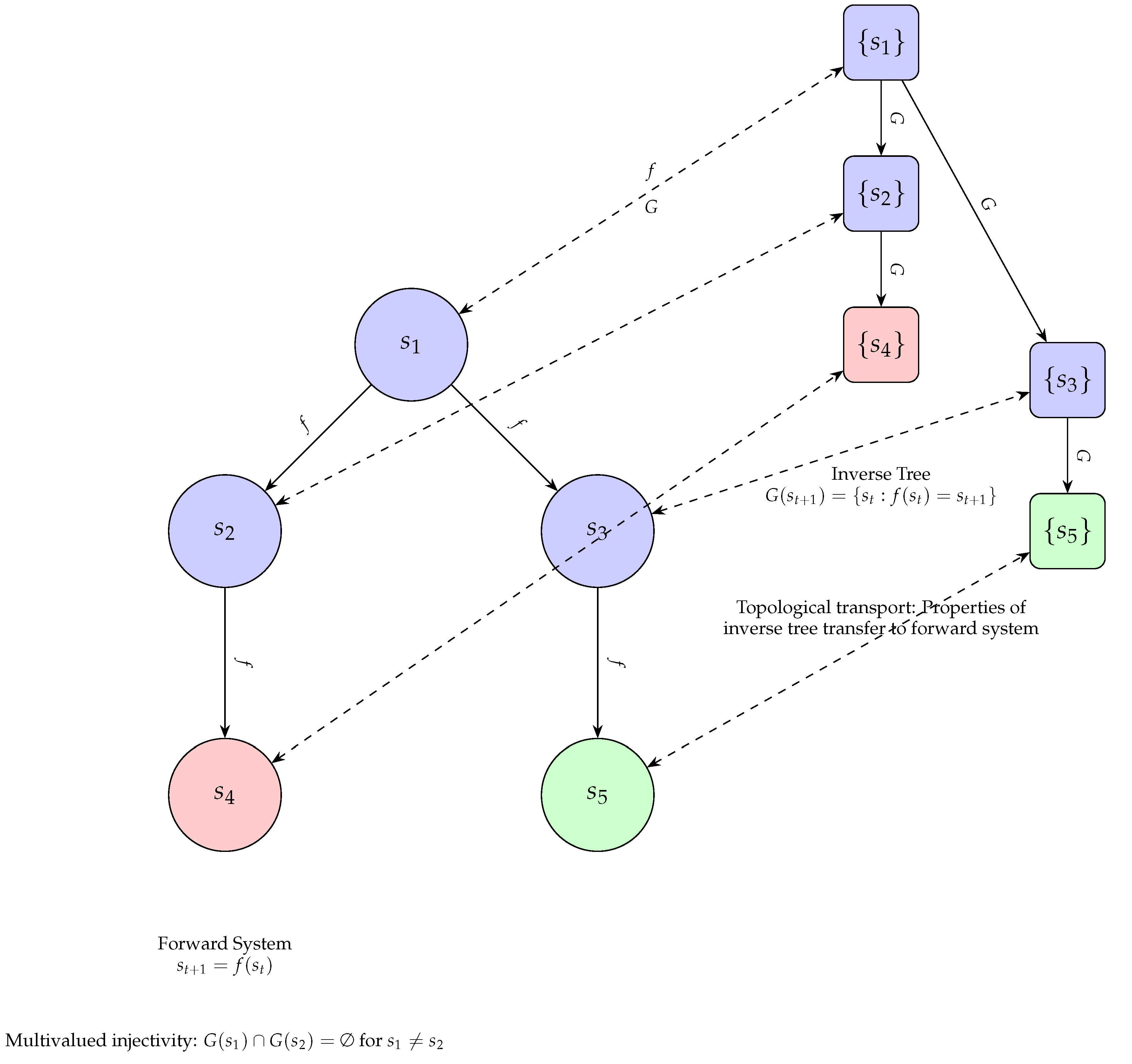
Figure 2.
Model of population growth (Inverse Forest).
Figure 3.
Models of evolutive network of genes.
Figure 4.
Inverse Tree .
Figure 5.
Inverse Tree .

Figure 6.
Inverse Tree .
Disclaimer/Publisher’s Note: The statements, opinions and data contained in all publications are solely those of the individual author(s) and contributor(s) and not of MDPI and/or the editor(s). MDPI and/or the editor(s) disclaim responsibility for any injury to people or property resulting from any ideas, methods, instructions or products referred to in the content. |
© 2024 by the authors. Licensee MDPI, Basel, Switzerland. This article is an open access article distributed under the terms and conditions of the Creative Commons Attribution (CC BY) license (http://creativecommons.org/licenses/by/4.0/).
Copyright: This open access article is published under a Creative Commons CC BY 4.0 license, which permit the free download, distribution, and reuse, provided that the author and preprint are cited in any reuse.


