1. Introduction
In the present era, software represents one of the most rapidly evolving domains. Companies are leveraging software as a core component for enhancing productivity, reducing costs, and exploring new markets. Today's software is providing more functionalities, processing bigger data and executing more complex algorithm compared to the past. Furthermore, it should interact with increasingly intricate external environments and must satisfy diverse constraints. Consequently, the scale and complexity of software exhibit swift escalation. Measurement data at Volvo showed that a Volvo vehicle in year 2020 had about 100 million LOC. This means that the vehicle had software equivalent to 6000 average books, which can be equivalent for a decent town library [
1].
As the scope and intricacy of software expand, ensuring its reliability becomes increasingly formidable [
2]. It is practically unattainable to detect and remediate of all defects within a given finite time and resources. Software defects refer to ‘errors or failures in software’ which could be resulted in inaccurate or unintended behavior and triggering unforeseen behaviors [
3,
4]. Quality management and testing expenditures aimed at guaranteeing reliability constitute a substantial portion of overall software development costs. The expense is escalating exponentially to rectify software defects in the later stages of development [
5]. Hence, utilizing available resources and minimize defects at the initial phase of a software development are crucial to obtaining high-quality outcomes [
6]. Such measures can curtail the expenses associated with defect rectification and mitigate the adverse ramifications of defects.
Software Defect Prediction (SDP) stands as a technique geared towards identifying flawed modules within source code, playing a crucial role in ensuring software quality [
7,
8]. SDP not only bolsters software quality but also economizes time and costs by concentrating testing resources to a heightened propensity of defects within constrained time and resources. Additionally, SDP augments testing efficiency by facilitating the identification of critical test cases and optimizing test sets effectively [
9]. Machine Learning-Based Software Defect Prediction (ML-SDP or SDP) represents a technological framework that leverages attributes gleaned from historical software defect data, software update records, and software metrics to train machine learning models for defect prediction [
8]. M. K. Thota [
8] envisions that ML-SDP will engender more sophisticated and automated defect detection mechanisms, emerging as focal points of research within the realm of software engineering.
Figure 1 elucidates the foundational process of SDP. The process includes collecting data (①), extracting features and labeling (②), training and testing models (③), and operationalizing the defect predictor for real-world application (④).
Nonetheless, the applicability of SDP models derived from previous research may encounter limitations when we directly transposed to industrial sectors. Disparities in software attributes and root causes of defects are apparent across various industry sectors, and even within a singular industrial sector. Discrepancies in software development methodologies and practices among projects can engender variations in software attribute and causes of defects. However, accessing real industrial sector data is often challenging as it is either not publicly available or difficult to obtain, making research challenging to utilize such data [
10]. Stradowski et al. [
11] underscore that although machine learning research aimed at predicting software defects is increasingly validated in industrial settings, there is still a lack of sufficient practical focus on bridging the gap between industrial requirements and academic research, which could help narrow the gap between them. Practical impediments, including disparities in software attributes, constraints in metric measurement, data scarcity, and inadequate cost-effectiveness, may impede the application of SDP methodologies from academic research to industrial sectors. Hence, we can facilitate the harnessing of SDP methodologies and foster future research initiatives via suggesting practical applicability, implementation and deployment of SDP through empirical case studies within industrial sectors.
In this research, we have endeavored to devise an SDP model leveraging data sourced from embedded software utilized in Samsung's telecommunication systems. To tailor the SDP model to the specific nuances of embedded software for telecommunication systems, we have introduced nine novel features. These features encompass six software quality metrics and three source code type indicators. Harnessing these features, we have trained a machine learning model to formulate the SDP model and scrutinized the impact of the new features on predictive efficacy to validate their effectiveness. Experimental outcomes revealed that the SDP model incorporating the nine new features exhibited a notable enhancement of 0.05 in both Recall and F-measurement metrics. Moreover, the overall predictive performance of the SDP model was characterized by an Accuracy of 0.8, Precision of 0.55, Recall of 0.74, and F-measurement of 0.63. This performance level is comparable to the average accuracy achieved across 11 projects as discussed by Kamei et al. [
12]. The results of this study confirm the contribution of the nine new features to predictive performance. Moreover, by examining the predictive contributions of each software quality metric, we can identify meaningful indicators for software quality management. Additionally, providing source codes to the machine learner resulted in enhanced predictive capability. These findings suggest that SDP can be utilized for early detection of software defects, efficient utilization of testing resources, and evaluation of the usefulness of software quality metrics in similar domains.
This paper adheres to the following structure: Chapter 2 delves into the theoretical underpinnings of Software Defect Prediction (SDP), reviews prior research in the field, and elucidates the limitations of previous studies. Chapter 3 encompasses an in-depth analysis of the characteristics of embedded software data pertinent to telecommunication systems, outlines the research questions, and delineates the experimental methodology employed. Chapter 4 scrutinizes the experimental findings and extrapolates conclusions pertaining to the research questions posited. Lastly, Chapter 5 expounds upon the implications and constraints of this study, alongside outlining avenues for future research endeavors.
3. Materials and Methods
3.1. Research Qeustion
In this study, we formulate the following four Research Questions (RQs):
RQ1. How effectively does the Software Defect Prediction (SDP) model anticipate defects?
Utilizing performance evaluation metrics such as Accuracy, Precision, Recall, F-measurement, and ROC-AUC Score, the performance of the SDP with embedded software for telecommunication system is compared with prior research findings.
RQ2. Did the incorporation of new features augment the performance of SDP?
Through a comparative analysis of performance before and after the integration of previously utilized features and novel features, and leveraging the Shapley Value to assess the contribution of new features, the significance of software quality indicators and source file type information is evaluated.
RQ3. How accurately does the SDP model forecast defects across different versions?
The predictive efficacy within the same version of the dataset, when randomly partitioned into training and testing subsets, is contrasted with predictive performance across distinct versions of the dataset utilized for training and testing. This investigation seeks to discern variances in defect prediction performance when trained on historical versions with defect data and tasted with predicting defects in new versions.
RQ4. Does predictive performance differ when segregating source files by type?
Software developers and organizational characteristics are important factors to consider in software defect research. F. Huang et al. [
37] analyzed software defects in 29 companies related to the Chinese aviation industry and found that individual cognitive failures accounted for 87% of defects. This suggests that individual characteristics and environmental factors may significantly impact defect occurrence. Source files are grouped based on software structure and software development organization structure, and the predictive performance is compared between cases where the training and prediction data are in the same group and cases where they are in different groups. This aims to ascertain the impact of source file type information on prediction accuracy.
3.2. Dataset
In this study, data originating from the base station software development at Samsung were utilized.
A base station serves as a wireless communication infrastructure facilitating the connection between user equipment (UE) and the core network, thereby enabling wireless communication services. The base station software, deployed within the base station, assumes responsibility for controlling the hardware of the base station and facilitating communication between mobile users and the base station itself. Its functionalities encompass signal processing, channel coding, scheduling, radio resource management, handover, and security protocols.
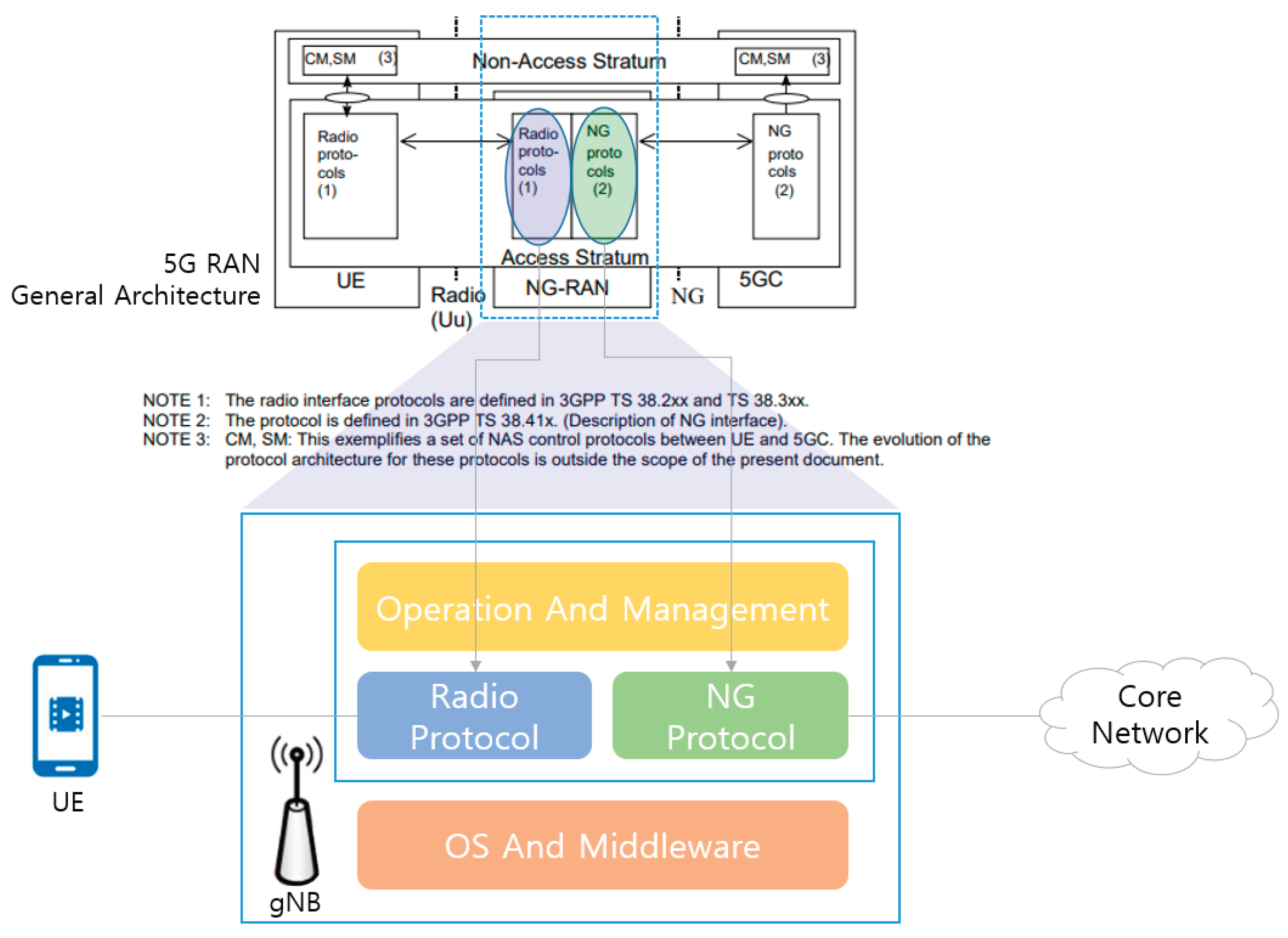
Figure 2 elucidates the structure of the base station software, illustrating the mapping relationship between the components of the base station software and the specifications outlined in the 3rd Generation Partnership Project Technical Specification (3GPP TS) 38.401 [
38].
The base station software undergoes continuous development of new versions. The development of 5G base station software, according to the roadmap of 5G mobile communication services, commenced around 2010 or earlier, with two or more packages being developed and deployed annually. Prior to the introduction of 5G mobile communication services, there existed 4G mobile communication services. Therefore, the development of 5G base station software involved extending the functionality of 4G base station software to support 5G services additionally. Consequently, if we consider the inclusion of 4G base station software, the development of base station software dates back to before 2000, indicating over 20 years of continuous development and deployment of new features.
The requirements for base station software stem from various factors.
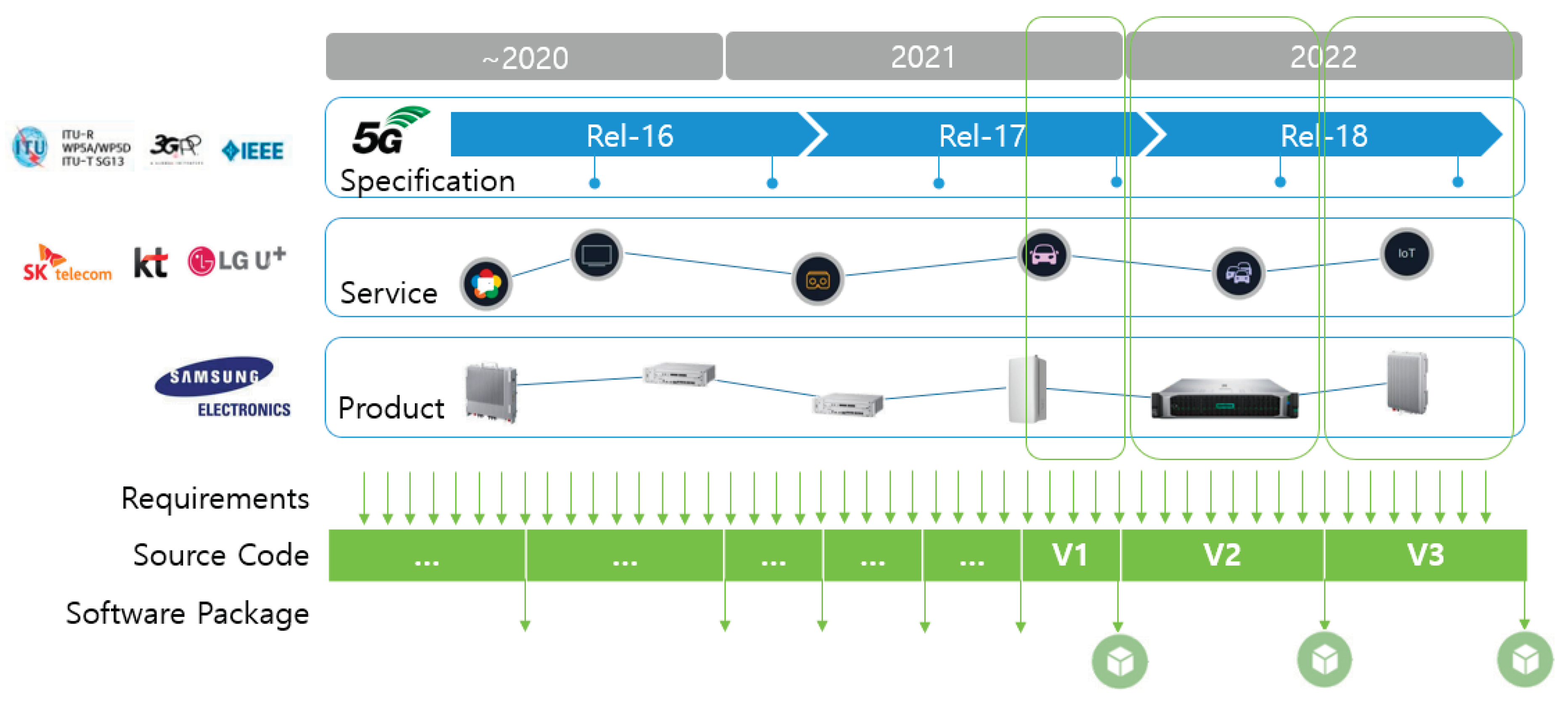
Figure 3 delineates the process that they are reflected on new versions of base station software.
The first set of requirements originates from international standardization organizations such as ITU-T, 3GPP, and IEEE. These organizations continually enhance existing standards and introduce new ones to align with advancements in wireless communication technology, thereby necessitating the development of base station software to accommodate these evolving specifications. The second set of requirements emerges from customers of base station systems, including network operators and service providers. These entities consistently pursue novel service development and service differentiation strategies to maintain a competitive advantage in the market. The requirements stemming from these endeavors drive the development of base station software to meet the evolving demands of customers. Lastly, internal demands within base station manufacturers contribute to requirements generation. In order to sustain a competitive edge in the market, base station manufacturers continuously innovate by developing new hardware products and introducing differentiated features compared to other manufacturers.
The requirements arising from these three sources are translated into features of the base station and are subsequently incorporated into the base station software. These additional base station features are then included in future base station software packages for deployment, ultimately facilitating the delivery of services to end-users, namely mobile subscribers, through deployment on operational base stations.
The base station software exhibits several characteristics. Firstly, due to continuous development of new versions over a period of more than 20 years, the existing code undergoes expansion and branching, leading to increased complexity and a higher likelihood of duplicate code. Secondly, differentiation demands from various customers result in multiple branches in the codebase, contributing to increased complexity and making code maintenance challenging. Thirdly, there is continuous development of new hardware models. The base station software is continuously expanded to support new hardware products, leading to increased code complexity to accommodate various models and address non-functional requirements such as real-time processing and memory optimization. This complexity results in features such as increased code complexity to support diverse models, preprocessing to reduce runtime image size, and the use of common memory to minimize data copying [
39,
40,
41,
42,
43]. Lastly, there are heterogeneous characteristics among subsystems and blocks of these software systems. The subcomponents of these systems possess unique software characteristics due to differences in technical domains and are developed by personnel with expertise in each technical domain. Examples of these technical domains include wireless communication technology, call processing, traffic processing, network management, and operating system and middleware technology.
In this study, three versions of base station software developed between 2021 and 2022 serve as the experimental dataset. The cumulative number of sample files across the three versions amounts to 17,727, with 3,993 instances (22.5%) exhibiting defects, labeled as Buggy files within their respective versions. Notably, there exist variations in both the number of samples and the Buggy Rate across the different versions. The codebase comprises a blend of C and C++ languages, with C constituting 60.7% and C++ encompassing 39.3% of the total codebase. Additionally, the Sample Rate denotes the proportion of files that were either newly created or modified relative to the total files, spanning a range from 40% to 74%. The Submitter count signifies the number of individuals involved in coding, ranging from 897 to 1,159 individuals. Furthermore, the Feature count denotes the tally of added or modified base station features, with 353, 642, and 568 features integrated in Versions 1, 2, and 3, respectively. The Development Period for each package is either 3 or 6 months.
Table 3.
The distribution of base station software development data across versions.
Table 3.
The distribution of base station software development data across versions.
| Version |
Samples
(Files) |
Buggy Files |
Buggy Rate |
Sample
Rate |
Code
Submitter |
Feature
Count |
Dev.
Period |
| V1 |
4,282 |
1,126 |
26.3% |
42% |
897 |
353 |
3M |
| V2 |
4,637 |
1,575 |
34.0% |
40% |
1,159 |
642 |
6M |
| V3 |
8,808 |
1,292 |
14.7% |
74% |
1,098 |
568 |
6M |
| Sum |
17,727 |
3,993 |
- |
- |
- |
- |
- |
| Average |
5,909 |
1,331 |
22.5% |
- |
- |
- |
- |
Table 4.
The distribution of base station software development data across programming languages.
Table 4.
The distribution of base station software development data across programming languages.
| Language |
Samples (Files) |
Buggy Files |
Buggy Rate |
| C |
8,585 |
2,188 |
20.3% |
| C++ |
5,149 |
1,805 |
26.0% |
| Sum |
17,727 |
3,993 |
- |
| Average |
5,909 |
1,331 |
22.5% |
3.3. Resrarch Design
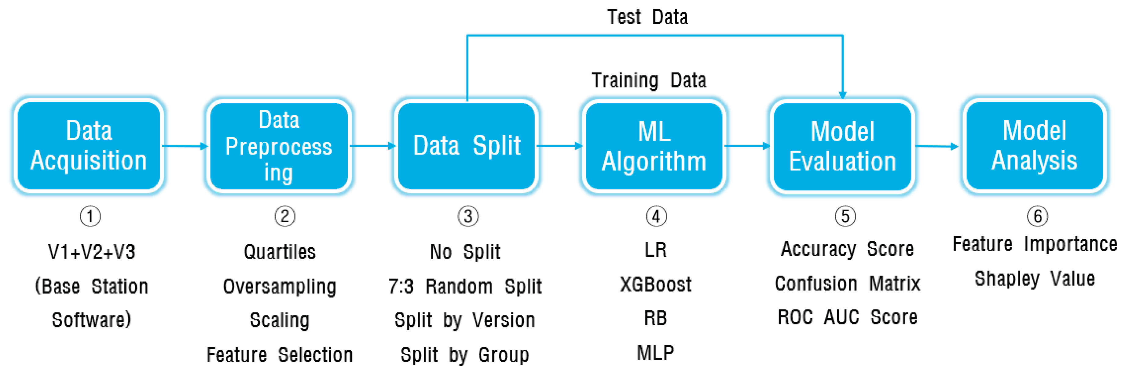
The experiments for developing the SDP model are organized into six distinct steps, each delineated to accomplish specific objectives.
Figure 4 provides an overview of the scope encompassed by each step within the experiment.
In the first data collection step (①), the recent data from the development projects of the base station software, encompassing the latest three versions, are gathered to be utilized as experimental data. The second data processing step (②) involves various tasks such as outlier correction based on Quartiles, oversampling to resolve class imbalance, scaling for uniformity in feature value ranges, appropriate feature selection for model construction, and data selection suitable for model building. In the third data splitting step (③), the training and testing data are divided using random splitting, version-based splitting, and specific group-based splitting methods. Version-based splitting is utilized for cross-version prediction, while group-based splitting is employed for experiments involving cross-group prediction. The fourth step (④) involves model selection, where machine learning algorithms like LR (Linear Regression), RB (Random Forest), XGB (XGBoost), and MDP are employed, and the model with the highest prediction performance is chosen. In the fifth step (⑤), model evaluation is conducted using metrics such as Accuracy, Precision, Recall, F-measurement, and ROC-AUC Score. Finally, in the sixth step (⑥) of model analysis, Feature Importance and Shapley Value are utilized to analyze the significance of features.
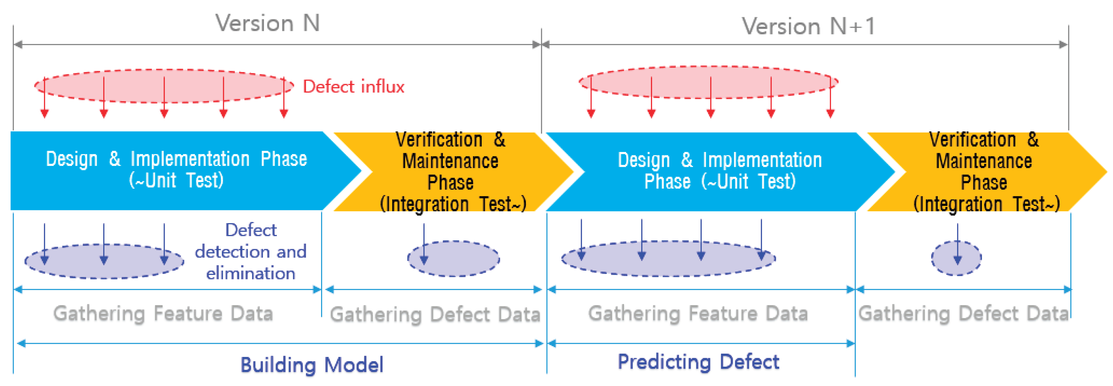
Figure 5 delineates the process of gathering training data and executing defect prediction in a scenario characterized by the continuous development of new software versions. Feature data and defect data acquired from version N serve as the training dataset for the machine learning model. Subsequently, the trained model is applied to predict defects using the feature data collected from version N+1.
In the design/implementation phase, both the introduction and removal of defects occur simultaneously. During this phase, defects are addressed through methods such as code reviews, unit testing, and other quality assurance practices. Ideally, all defects introduced during the design/implementation phase should be removed before the verification/maintenance phase. Defects that are not addressed during the design/implementation phase are detected during the verification/maintenance phase. Machine learning is then employed to learn the characteristics of modules containing these defects. In the design/implementation phase of version N+1, software defect prediction (SDP) is used to identify modules similar to those in version N that experienced defects, categorizing them as likely buggy modules with similar characteristics.
3.4. Software Metrics
Software metrics quantify the characteristics of software into objective numerical values and are classified into Project metrics, Product metrics, and Process metrics [
44]. In this study, Product metrics and Process metrics are utilized as features for machine learning training. Product metrics pertain to metrics related to product quality assessment and tracking. Representative examples of Product metrics include code complexity and the number of lines of code. Process metrics, on the other hand, relate to process performance and analysis. Examples of Process metrics accumulated during the development process include code change volume, code commit count, and number of coding personnel. Raw data collected from software quality measurement systems consist of metrics at both the function and file levels, necessitating the transformation of function-level metrics into file-level metrics. The "min/max/sum" in the “Comments” field of the table indicate the conversion of function-level metrics to the corresponding file-level metrics. Additionally, identifiers such as subsystem identifier, block identifier, and language identifier are employed to differentiate between file types. Subsystems represent the subcomponents of software systems, while blocks are subcomponents of subsystems.
In this study, the selection of features was guided by established metrics validated in prior research, aligning with Samsung's software quality management policy, which encompasses quality indicators and source file type information. Given the amalgamation of C and C++ programming languages within the codebase, we considered metrics applicable to both languages. Our feature set encompassed foundational software metrics such as code size, code churn, and code complexity, complemented by additional metrics specified by Samsung's software quality indicators to bolster prediction efficacy. Additionally, we extracted subsystem and block information, representing the software's hierarchical structure, from the file path information. To account for the mixed presence of C and C++ files, we also incorporated identifiers to distinguish between them. The added metrics are highlighted in gray in
Table 5 above.
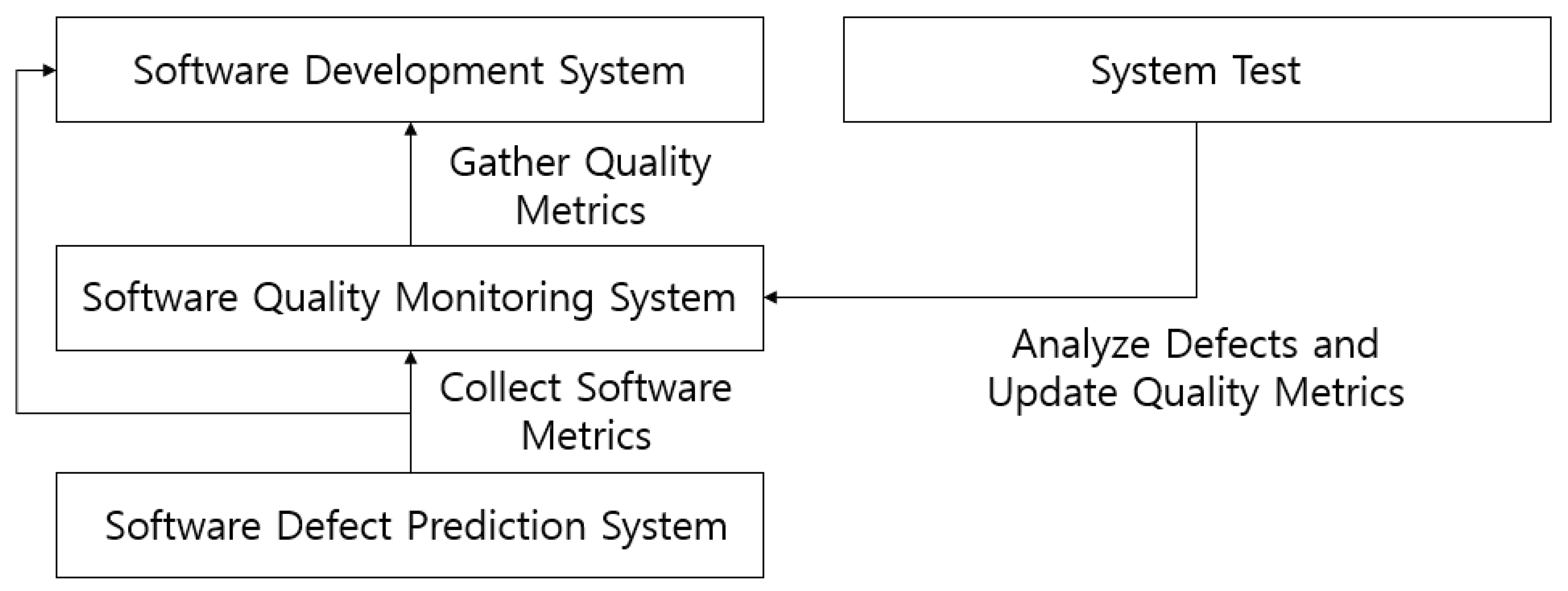
Metrics derived from Samsung's software quality indicators include GV (Global Variable), MCD (Module Circular Dependency), DC (Duplicate Code), and PPLoc (Pre-Processor Loc). These metrics were derived by analyzing defects identified during system testing by the software validation department.
Figure 6 illustrates the process of measuring metrics in the software development process and improving metrics based on defect prevention. The software quality management system periodically measures quality metrics, including metrics related to code. When defects are detected during system testing, an analysis of these defects is conducted, leading to the derivation of metrics for proactive defect detection. These metrics are then added back into the software quality management system's quality indicators and measured regularly.
In industrial software development projects, domain-specific metrics are frequently utilized to bolster prediction accuracy. Many of those metrics were omitted from this study due to disparities in development methodologies or insufficient data accumulation. For instance, metrics such as EXP (Developer Experience), REXT (Recent Developer Experience), and SEXP (Developer Experience on a Subsystem) employed by Kamei [
12] were not integrated into our research. Instead, to better align with the attributes of embedded software for telecommunication systems, we introduced nine supplementary features, as delineated below.
GV (Global Variable) represents the count of global variables in each file that reference variables in other files. Global variables increase dependencies between modules, deteriorating maintainability, and making it difficult to predict when and by which module a value is changed, thereby complicating debugging. Therefore, it is generally recommended to use global variables at a moderate level to minimize the risk of such issues. However, in embedded software, there is a tendency for increased usage of global variables due to constraints in speed and memory.
MCD (Module Circular Dependency) indicates the number of loops formed when connecting files with dependencies. Having loops deteriorates the maintainability of the code, so it is recommended to avoid creating loops. In the case of large-scale software development, such as communication system software, where multiple developers work on it for extended periods, these dependencies can unintentionally arise.
DC (Duplicate Code) represents the size of repetitive code. When there is a lot of duplicate code, there is a higher risk of missing modifications to some code during the maintenance process, which can be problematic. Therefore, removing duplicate code is recommended. Embedded software for communication systems tends to have a large overall codebase, and the code continuously expands to support new hardware developments. At the same time, development schedules may not allow sufficient time for timely market releases, and there is less likelihood of the same developer consistently handling the same code. In such environments, developers may not have enough time to analyze existing code thoroughly, leading them to copy existing code to develop code for new hardware models, resulting in duplicate.
PPLoc (PreProcessor Loc) is the size of code within preprocessor directives such as #ifdef... and #if.... These codes are determined for compilation inclusion based on the satisfaction of conditions written alongside preprocessor directives during compile time. In embedded software for communication systems, due to memory constraints of hardware devices like DSPs (Digital Signal Processors), codes executing on each hardware are included in the execution image to minimize code size. For this purpose, preprocessor directives are employed. However, similar to DC, this practice leads to the generation of repetitive, similar codes, increasing the risk of missing modifications to some codes during code editing.
cov_l and cov_b respectively represents Line Coverage and Branch Coverage, indicating the proportion of tested code out of the total code. A lower proportion of tested code in developer testing increases the likelihood of defects being discovered during system testing.
Critical/Major denotes the number of defects detected by static analysis tools. If these defects are not addressed by the developer testing phase, the likelihood of defects being discovered during system testing increases.
FileType serves as an identifier for distinguishing between C code and C++ code. It is a feature aimed at incorporating the differences between C and C++ code into machine learning training.
Group_SSYS serves as information to identify subsystems. Subsystems are subunits that constitute the entire software structure. This feature enables the machine learning model to reflect the differences between subsystems in its training.
Group_BLK serves as information to identify blocks. Blocks are subunits that constitute subsystems in the software structure. This feature enables the machine learning model to reflect the differences between blocks in its training.
3.5. Defect Labeling
The defect labels are determined based on the defect information described in the Code Commit Description. In reality, it is challenging to manage defect information in a way that enables perfect tracking of defect codes in industrial domains. Defect tracking requires additional effort, but it is often difficult to allocate resources for this purpose. Therefore, it is necessary to find the optimal solution tailored to the specific development processes and practices of each domain or organization. In this study, Code Commit Descriptions were subjected to text mining to classify Code Commits containing topics highly relevant to defects as code commits resulting from defect fixes.
3.6. Mitigating Class Imblance
The data used in this study contains class imbalance, with the Buggy class accounting for 22.5% of the data. This imbalance arises because the proportion of actual buggy code in the entire source code is significantly lower than that of clean code. Balancing class ratios is an important step to improve prediction performance in software defect prediction. In software defect prediction, the goal is to increase Recall, which measures the model's ability to predict actual defects, and to reduce the False Positive (FP) rate, which represents the proportion of non-defective classes misclassified as defective among all non-defective classes. With the advancement of machine learning technology, various techniques have been proposed to address class imbalance. In the field of software defect prediction, SMOTE (Synthetic Minority Over-sampling Technique) [
45,
46] is commonly used, but research is ongoing to further enhance prediction performance, including studies applying GAN models [
27,
47]. In this study, we utilize SMOTEENN, a technique that combines over-sampling and under-sampling methods.
3.7. Machine Learning Models
Software defect prediction can be approached using various machine learning models. Research in this area aims to compare the performance of different models, identify the most superior model, or analyze the strengths and weaknesses of each model to guide their selection for real-world industrial domain applications. In this study, LR (Logistic Regression), RF (Random Forest), and XGB (XGBoost) [
48], which are commonly used in industrial domain applications and offer interpretable prediction results, are used as the base models. Additionally, MLP (Multilayer Perceptron) is employed to evaluate prediction performance. Among these models, XGB exhibited the most superior performance in this study and was selected as the SDP model.
3.8. Model Performance Assessment
Performance evaluation metrics widely used in software defect prediction include Accuracy, Precision, Recall, F-measure, and ROC-AUC Score.
Table 6 presents the confusion matrix used to define these performance evaluation metrics. In this study, the goal is to increase both Recall and Precision, which together contribute to F-measure, reflecting the model's ability to predict defects among actual defects in software defect prediction.
Accuracy (ACC) quantifies the proportion of accurately predicted instances relative to the total number of instances.
Precision delineates the ratio of accurately predicted positive instances to the total number of instances classified as positive.
Recall signifies the ratio of accurately predicted positive instances to the total number of actual positive instances.
F-measure amalgamates both Precision and Recall, calculated as the harmonic mean of the two values.
3.9. Feature Importance Analysis
Feature importance analysis aims to determine how much each feature contributes to predictions. In this study, Feature Importance and Shapley Value are used to assess the importance of features.
Shapley Value [
49,
50], derived from Coalitional Game Theory, indicates how much a feature contributes to the model's predictions. This concept helps measure the importance of each feature and interpret the model's prediction results. To understand how much a specific feature contributes to predictability, Shapley Value calculates the contribution of a particular feature by comparing scenarios where the feature is included and excluded in all combinations of features.
Shapley Value is defined through the following Value Function. The Shapley value of features in set S represents their contribution to the predicted value, assigning weights to all possible combinations of feature values and summing them. The contribution of using all features equals the sum of the contributions of individual features.
3.10. Cross-Version Performance Measurement
In this study, an SDP model is constructed using the complete dataset comprising three versions: V1, V2, and V3. The dataset is randomly partitioned, with 70% allocated for training purposes and the remaining 30% for testing. Subsequently, the finalized SDP model is deployed within an environment characterized by continuous software development, leveraging historical version data to train and predict faulty files in newly developed iterations. Consequently, cross-version performance assessment entails scrutinizing and interpreting variations in prediction efficacy when employing data from preceding versions for training and subsequent versions for testing.
Although the optimal scenario would entail training with data from past versions (Vn) and testing with data from the succeeding version (Vn+1) to gauge cross-version performance comprehensively, the limited availability of data spanning solely three versions necessitate a more nuanced approach. Hence, experiments are executed by considering all feasible permutations of versions, wherein each version alternately serves as both training and testing data, facilitating a comprehensive evaluation of cross-version performance.
3.11. Cross-Group Performance Measurement
Large-scale software can exhibit different software characteristics among its subcomponents, each contributing to the overall functionality. In the software utilized in this study, with over a thousand developers, the technical domains of the software are distinctly categorized into wireless protocols, NG protocols, operations management, and OS and middleware. Leveraging the file path information, the entire dataset is segmented into several groups with identical features. Cross-group performance measurements are then conducted to ascertain whether there are differences in characteristics among these groups.
Figure 7 illustrates the method of instance grouping.
To separate groups using path information, the paths are tokenized into words and then vectorized using TF-IDF (Term Frequency Inverse Document Frequency) (②). Subsequently, K-NN clustering is applied to the vectorized path information to cluster similar paths into five groups (four representative subsystem codes + miscellaneous code) (③). Defining groups in this manner allows for the identification of differences in characteristics among the groups. When such differences are observed, adding group information as a feature to the model can provide additional information, thereby potentially improving prediction performance.
Table 7.
Distribution of base station software data groups (subsystems).
Table 7.
Distribution of base station software data groups (subsystems).
| Group |
Samples (Files) |
Buggy Files |
Buggy Rate |
| G0 |
3,999 |
1,321 |
24.8% |
| G1 |
3,477 |
1,319 |
27.5% |
| G2 |
1,743 |
328 |
15.8% |
| G3 |
2,118 |
263 |
11.0% |
| G4 |
2,397 |
762 |
24.1% |
| Sum |
17,727 |
3,993 |
22.5% |
4. Results
In this chapter, we delve into addressing the four Research Questions (RQs) delineated in
Section 3.1, leveraging insights gleaned from the experimental outcomes.
Answer for RQ1. How effectively does the Software Defect Prediction (SDP) model anticipate defects?
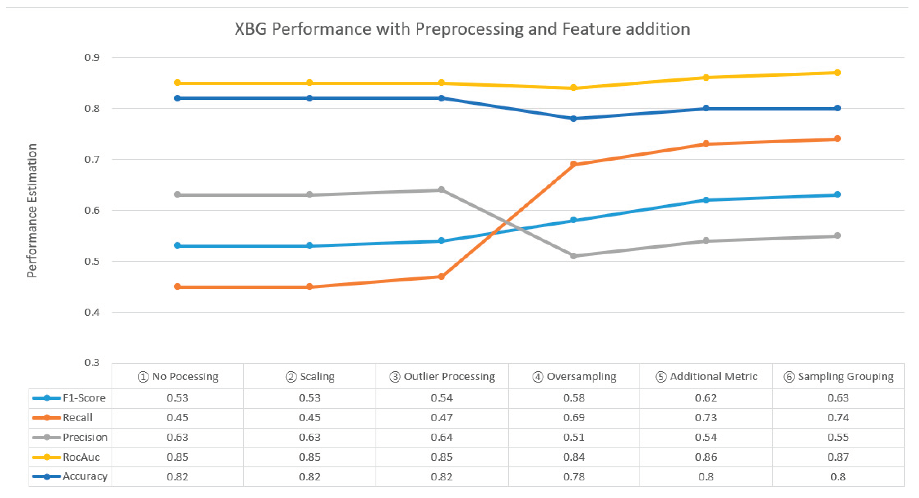
Table 8 showcases the performance measurement outcomes of the XGB-based SDP model across six distinct scenarios. Initially, performance evaluation was conducted without any data preprocessing (①), followed by successive additions of scaling (②), outlier removal (③), class imbalance resolution through oversampling (④), incorporation of new metrics (⑤), and eventually the addition of file type information (⑥). The ML-SDP exhibited its optimal performance when comprehensive preprocessing was applied, incorporating all new features, and employing the XGB classifier. In this scenario, the performance metrics were as follows: Recall of 0.63, F-measurement of 0.74, and ROC-AUC Score of 0.87.
In comparison with prior studies, the predicted performance displayed notable variations, with some studies indicating higher performance and others demonstrating lower performance compared to our experiment.
Table 9 provides a comparative analysis of our results with those from previous studies. Among twelve prior studies including seven on open-source projects and 5 on industrial domain projects, our study exhibited lower performance than six studies and comparable performance to six studies. Thus, it can be inferred that the ML-SDP model developed using Samsung's embedded software for telecommunication system has achieved a meaningful level of performance.
Answer for RQ2. Did the incorporation of new features augment the performance of SDP?
Figure 8 provides a visual representation of the changes in predictive performance resulting from data processing and feature addition. Before incorporating the six new metrics and three source file type information, the performance metrics were as follows: Precision 0.51, Recall 0.69, F-measurement 0.58, Accuracy 0.78, and ROC-AUC Score 0.84. Subsequently, after integrating the new metrics and source file type information, the performance metrics improved to Precision 0.55, Recall 0.74, F-measurement 0.63, Accuracy 0.80, and ROC-AUC Score 0.87. After introducing the new metrics, all five indicators exhibited improvement. Upon closer examination of the F-measure, there was a 6.90% increase from 0.58 to 0.62 (⑤) and upon the inclusion of three additional source file types, four out of the five indicators showed further enhancement, resulting in a 1.72% increase from 0.62 to 0.63 (⑥). Overall, the total increase amounted to 0.86%. It is evident that the additional features introduced in this study significantly contributed to the enhancement of the predictive power of the SDP model.
The examination of feature contributions, as depicted in
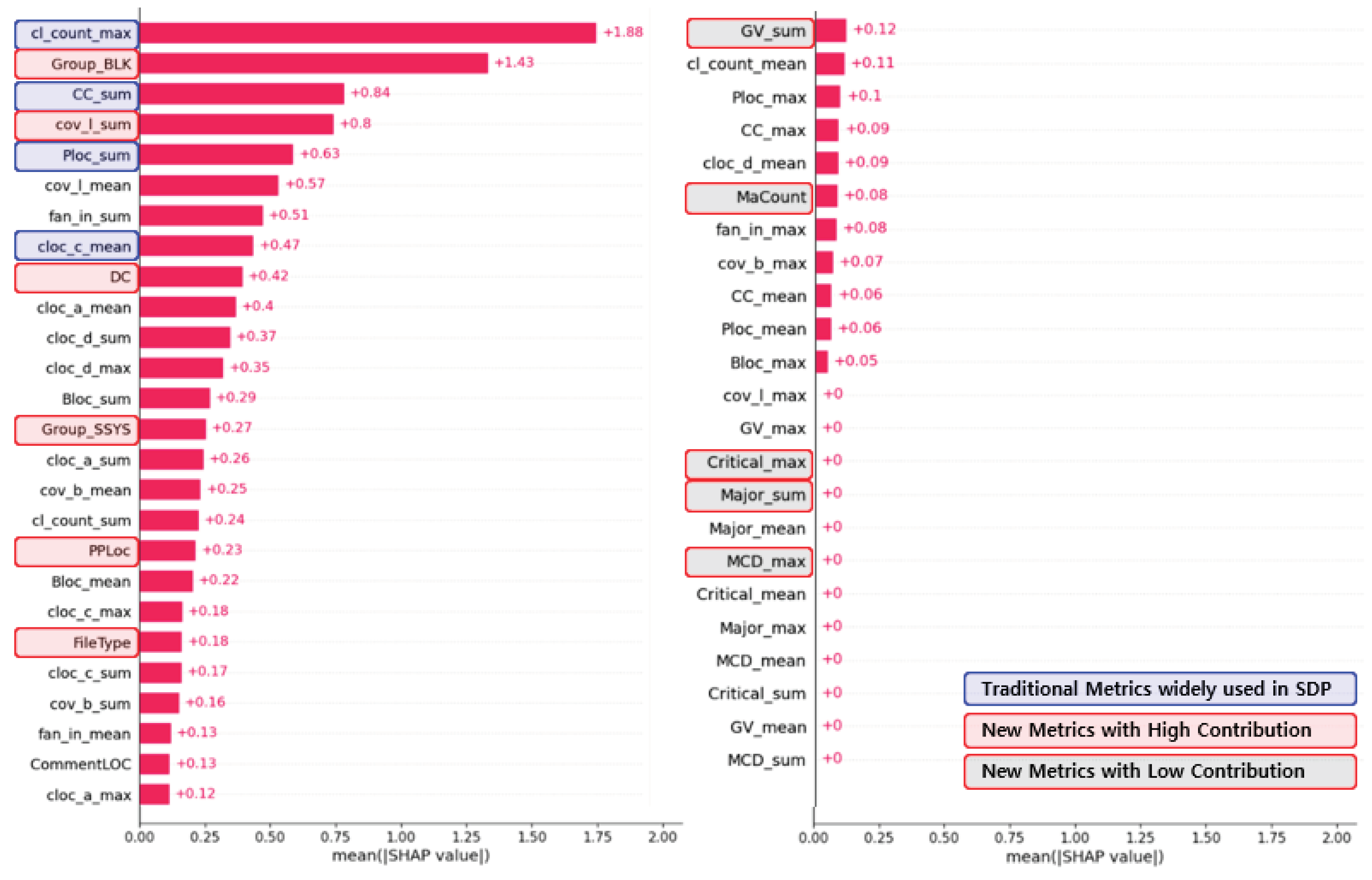
Figure 9, reveals notable insights into the predictive power of various metrics. The contributions of traditional and widely used metrics in SDP, such as BLOC (Build LOC), CLOC (Changed LOC), and CC (Cyclomatic Complexity) remained still high. However, some of the new features such as Group_BLK, cov_l (Line Coverage), DC (Duplicate Code), Group_SSYS, and PPLoc also played an important role in improving prediction performance. Meanwhile GV, Critical/Major, and MCD features show only minimal contributions.
Moreover, the Shapley Value analysis underscored the pivotal role of certain quality metrics in capturing fault occurrence trends. Specifically, Coverage, DC, and PPLoc displayed robust associations with fault occurrence, affirming their effectiveness as indicators for quality enhancement initiatives. On the contrary, GV, Critical/Major, and MCD features demonstrated minimal associations with fault occurrence, implying their limited utility in defect prediction scenarios. These findings provide actionable insights for prioritizing metrics and refining defect prediction strategies to bolster software quality.
Answer for RQ3. How accurately does the SDP model forecast defects across different versions?
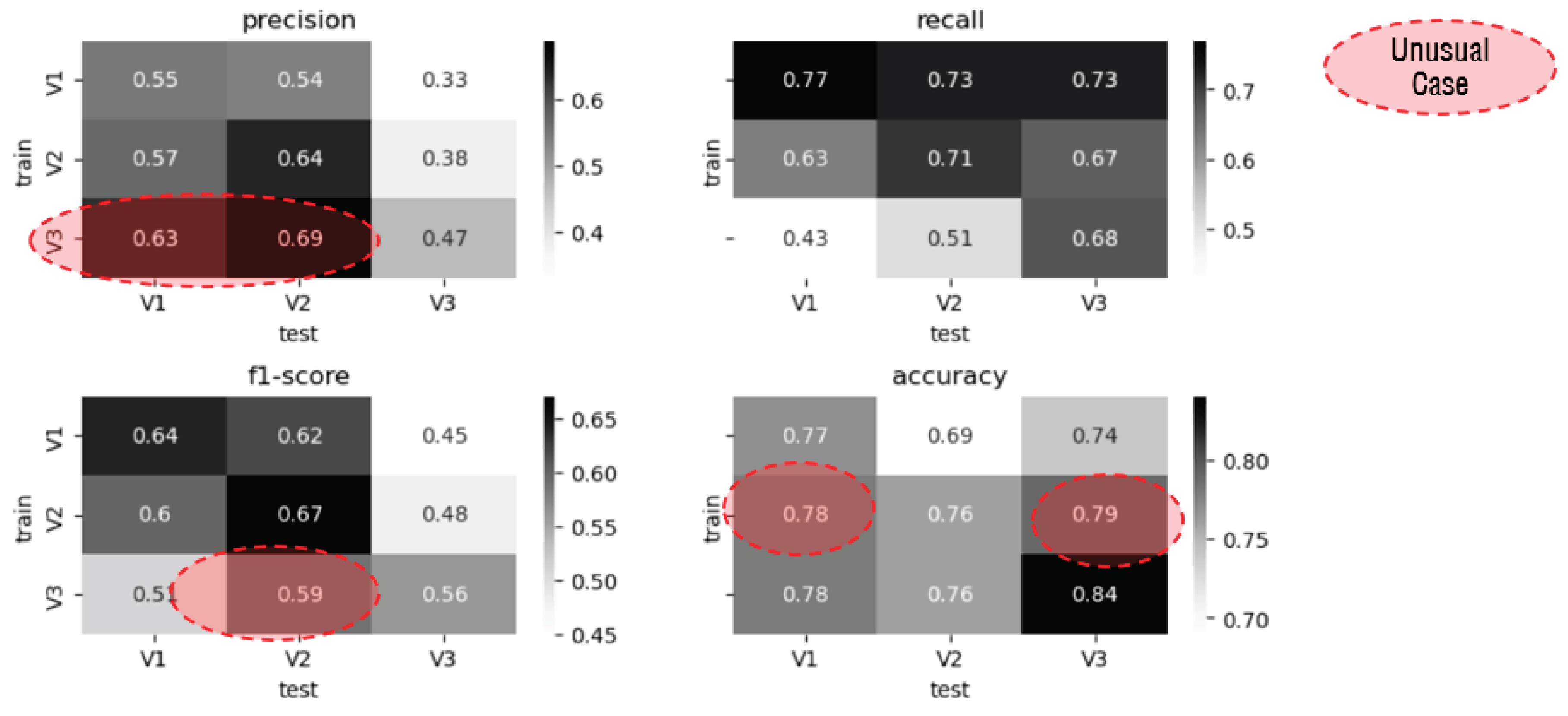
The comparative analysis of prediction performance across both same-version and cross-version scenarios yielded insightful observations. Precision metrics revealed that, among the six cross-version predictions, four exhibited lower values than their same-version counterparts, while two displayed higher values. Similarly, Recall metrics indicated consistently lower performance across all six cross-version predictions. F-measurement metrics exhibited lower values in five out of six cross-version cases and higher values in one case. Accuracy metrics followed a similar trend, with lower values observed in four cases and higher values in two cases compared to the same-version predictions.
Overall, the average prediction performance under cross-version conditions demonstrated a notable decline across all five metrics compared to the same-version predictions. Particularly noteworthy was the average F-measurement (f1-score), which decreased from 0.62 for the same version to 0.54 for cross-version predictions, reflecting a significant 13% decrease in prediction performance.
The observed deterioration in prediction performance under cross-version conditions underscores the presence of distinct data characteristics among different versions. It also suggests that the anticipated prediction performance under cross-version conditions is approximately 0.54 based on the F-measurement metric. These findings highlight the importance of considering version-specific nuances and adapting prediction models accordingly to maintain optimal performance across diverse software versions.
Table 10.
Comparison of Prediction Performance under Cross-Version Conditions.
Table 10.
Comparison of Prediction Performance under Cross-Version Conditions.
| Case |
Precision |
Recall |
F-measurement |
Accuracy |
ROC-AUC |
| Average for Within Version |
0.55 |
0.72 |
0.62 |
0.79 |
0.86 |
| Average for Cross Version |
0.52 |
0.62 |
0.54 |
0.76 |
0.81 |
Figure 10.
Prediction Performance under Cross-Version.
Figure 10.
Prediction Performance under Cross-Version.
Answer for RQ4. Does predictive performance differ when segregating source files by type?
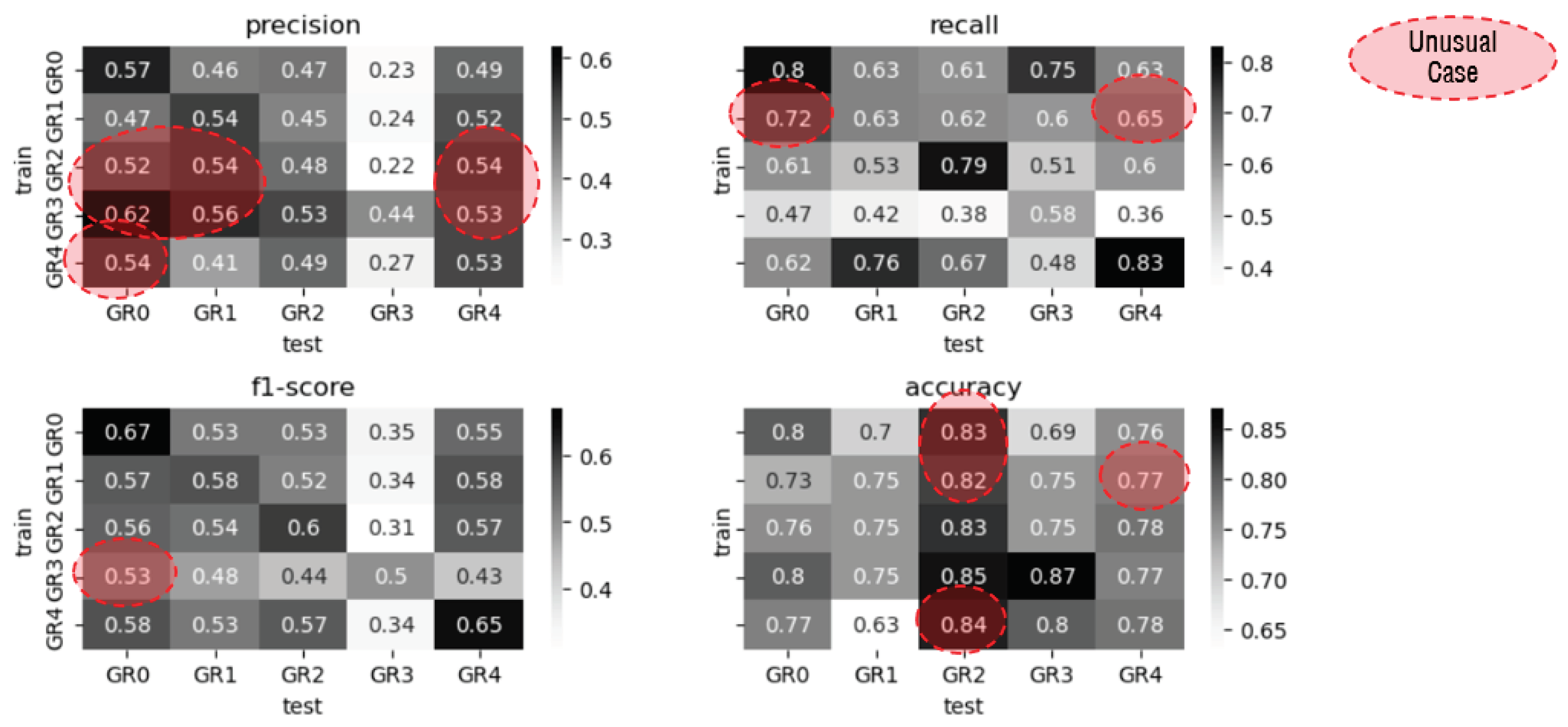
The analysis of prediction performance across cross-group scenarios revealed notable trends. Among the 20 cross-group predictions, 13 exhibited lower Precision compared to the same group, while 7 showed higher Precision. Similarly, 18 predictions demonstrated lower Recall, with only 2 displaying higher values. F-measurement scores followed a similar pattern, with 19 predictions showing lower values and 1 demonstrating improvement. Accuracy metrics indicated lower values in 16 cases and higher values in 4 cases compared to the same group predictions.
On average, predictive performance under cross-group conditions was consistently lower across all five metrics compared to the same group predictions. Specifically, the average F-measurement for the same group was 0.60, while for cross-group predictions, it decreased to 0.50, reflecting a notable 17% decrease in predictive performance.
The observed decline in predictive performance under cross-group conditions underscores the significance of variations in data characteristics among different groups. To address this, we incorporated source file type information for group identification.
Figure 8 demonstrates that the addition of source file type information resulted in a 1% improvement in Precision, Recall, and F-measurement metrics, indicating its effectiveness in enhancing prediction performance across diverse group scenarios.
Table 11.
Comparison of Prediction Performance under Cross-Group Conditions.
Table 11.
Comparison of Prediction Performance under Cross-Group Conditions.
| Case |
Precision |
Recall |
F-measurement |
Accuracy |
ROC-AUC |
| Average of Within Group |
0.51 |
0.73 |
0.60 |
0.81 |
0.85 |
| Average of Cross Group |
0.46 |
0.58 |
0.50 |
0.77 |
0.79 |
Figure 11.
Prediction Performance under Cross-Group.
Figure 11.
Prediction Performance under Cross-Group.
5. Conclusions
The study proposes an SDP model tailored for Samsung's embedded software in telecommunication systems, yielding several significant results and implications. Firstly, it validates the applicability of SDP in the practical realm of embedded software in telecommunication systems. The model demonstrated moderate performance levels compared to existing research, with F-measurement at 0.63, Recall at 0.74, and Accuracy at 0.80. Secondly, specialized features like DC and PPLoc, specific to Samsung, were found to enhance predictive performance, leading to an increase in F-measurement from 0.58 to 0.62. Thirdly, the inclusion of three file type information of subsystem, block and language identifiers as features for machine learning training contributed to performance improvements, evidenced by an increase in F-measurement from 0.62 to 0.63. Lastly, the study quantitatively confirmed the significance of Samsung's software quality metrics as indicators of software quality, enhancing predictive performance when incorporated as features.
Our SDP model has been adopted to the real projects to evaluate the effectiveness of software quality metrics, implement Just-in-Time Buggy module detection [
51], and enhance test efficiency through recommendations for buggy module-centric test cases. The model is aiding developers in identifying faulty modules early, understanding their causes, and making targeted improvements such as removing duplicate code and optimizing preprocessing directives.
The study has successfully developed the ML-SDP model tailored for embedded software in telecommunication systems, highlighting its applicability in similar domains and the effectiveness of novel features. However, several avenues for further research and expansion are identified. Firstly, there is a crucial need to delve into cases where predicted values deviate from actual values. Investigating such instances, pinpointing the underlying causes of discrepancies, and mitigating prediction errors can significantly enhance the accuracy of predictions. Secondly, it is imperative to explore the applicability of advanced methods known to enhance prediction performance in real-world industrial settings. One promising direction is the utilization of SDP models leveraging Transformer, a cutting-edge Deep Learning (DL) technology.
