Submitted:
07 March 2024
Posted:
08 March 2024
You are already at the latest version
Abstract
The dust originating from the extinct lake of the Aral Sea poses a considerable threat to the sur-rounding communities and ecosystems. The accurate location of these wind erosion areas is an essential prerequisite for controlling sand and dust activity. However, few relevant indicators re-ported in the current study can accurately describe and measure wind erosion intensity. A novel wind erosion intensity (WEI) of a resolution unit was defined in this paper based on the deformation due to the wind erosion in this resolution unit. We also derived the relationship between WEI and soil InSAR temporal decorrelation (ITD). The ITD is usually caused by the surface change over time, which is very suitable for describing wind erosion. However, within one resolution unit, the ITD signal usually includes soil and vegetation contributions, and few studies are referred to this. Therefore, we proposed an ITD decomposition model (ITDDM) to decompose the ITD signal of a resolution unit. The least-squares method (LSM) based on singular value decomposition (SVD) is used to estimate the ITD of soil (SITD) within a resolution unit. We verified the results qualitatively by the landscape photos, which can reflect the actual conditions of the soil. At last, the WEI of the Aral Sea from June 23, 2020, to July 05, 2020, was mapped. The results confirmed that (1) Based on the ITDDM model, the SITD can be accurately estimated by the LSM method, (2) the Aral Sea is experiencing severe wind erosion, and (3) The middle, northeast, and southeast bare areas of the South Aral Sea are where salt dust storms may occur.
Keywords:
Aral Sea
; InSAR temporal decorrelation
; backscattering coefficient
; wind erosion
; dust storms
1. Introduction
The fine particles produced by wind erosion are
essential for sand and dust activities. The sand and dust activities,
especially the salt dust activities, are a disaster for surrounding residents
and ecosystems in the Aral Sea [1]. Wind
erosion accelerated the desertification process and promoted the formation of
the Aralkum Desert. Sufficient fine particles from this new desert provide
favorable conditions for sand and dust activities. The salt storms generated by
winds caused various diseases to the surrounding residents and result in the
death of a large area of vegetation, especially the crops. Accurate
localization of these wind erosion areas is necessary for human intervention in
salt and dust storms. Scientists developed numerous models based on traditional
experimental physics and remote sensing technology to distinguish different
degrees of wind erosion.
Wind erosion research results based on traditional
experimental physics provide a solid theoretical foundation for wind erosion
research. According to the study of Liu and Zobeck based on experimental
physics methods, wind blowing, impact and abrasion of moving particles are the
three primary forms of particle moving and separation [2,3]. Bagnold derived the threshold of the starting
wind speed of the particle fluid according to the moment balance equation [4]. The research results of Lu and Shao show that
when the ground particles are mainly dust, the vertical dust flux caused by the
impact is proportional to the 3-4 power of the wind speed [5]. Numerous scientists have studied the forms and
laws of the movement of sand and dust and provided many physical models of
different forms of movement [3,6–15].
Particles suspended in the air fall to the ground mainly through dry and wet
sedimentation. The physical processes involved in dry and wet sedimentation are
relatively complex, and there is no effective means to describe the dry and wet
sedimentation process [6,16–18]. Clarifying
the influencing factors of the wind erosion process is the basis for
establishing the wind erosion model, and Chepil’s classification of wind
erosion factors plays an essential role in advancing the research on the wind
erosion process [19]. Based on Chepil’s
research results, subsequent researchers have proposed many well-known wind
erosion models [20–25]. The research of wind
erosion process based on traditional experimental physics has essential value
and significance for human understanding of the fundamental laws of wind
erosion activity. However, the uncertainty of the wind erosion model itself and
the difficulty of obtaining high spatial and temporal resolution data greatly
limit the wind erosion model in the application of describing large-scale wind
erosion scenarios.
InSAR (Interferometric
Synthetic Aperture Radar) decorrelation can be used to describe the random
changes of the surface due to wind erosion, expecting to solve the problem of
quantitative characterization of the wind erosion intensity [26]. Coherence is commonly employed to assess
the similarity of InSAR echo signals. It quantifies the correlation between two
complex InSAR echo signals by calculating their correlation coefficient.
Computation of radar echo signal coherence typically involves spatial averaging
of the radar echo signals within a moving window. Decorrelation, numerically
equal to 1 minus the coherence coefficient, denotes the loss of coherence.
Various factors contribute to decorrelation, including temporal, thermal, and
spatial. Estimating temporal decorrelation involves eliminating the impacts of
thermal and spatial decorrelation from the total decorrelation [27].
In 1992, Zebker and Villasenor studied the
relationship between ITD and surface erosion of the Death Valley in California,
and the results showed that ITD and wind erosion degrees have a negative linear
correlation. In another study in 2000, Wegmuller confirmed this relationship,
and he pointed out that the above relationship is still valid when the
vegetation coverage is less than 40% [28].
Later, InSAR decorrelation was used to study the desertification due to wind
erosion, also showing that this technology has the ability to detect ground
changes due to wind erosion [29–31]. In some
other studies related to dune stability, it has been confirmed that temporal
decorrelation technology can detect changes in the surface of dunes due to wind
erosion [32,33].
Although many indicators in the current study were
proposed to describe the WEI, few can be used to describe and measure the WEI
of a resolution unit accurately. This paper proposed a novel WEI of a
resolution unit based on the surface deformation caused by wind erosion.
Zebker’s research shows that the ITD in the resolution unit is related to the
displacement of scatters in it [26]. Based on
the relationship between scatters’ random displacement and the surface random
deformation within a resolution unit, we related the WEI with the SITD of a
resolution unit. In fact, the resolution unit’ ITD often involves the
contribution of soil and vegetation in the bare lands of the Aral Sea.
Wegmuller’s study indicates that the ITD of a resolution unit was equal to the
sum of the weighted ITD of all scatterers within the resolution unit [28]. However, few studies are involved in
decomposing the ITD contributions of all scatterers within a resolution unit.
Therefore, this paper focuses on the:
- Model the WEI of a resolution unit and relate the WEI with the SITD of this resolution unit.
- SITD estimation within a resolution unit.
- Mapping the WEI of the dry lakebed of the Aral Sea.
2. Study Area
Part of the Aral Sea is in southern Kazakhstan, and
the rest is in northern Uzbekistan. Due to the extended distance from the sea,
the Aral Sea has a classical continental dry climate. The study area is shown
in Figure 1.
Figure 1.
Study area and the corresponding land types. The 2017 land surface coverage map with a resolution of 10 m is from Tsinghua University (http://data.ess.tsinghua.edu.cn/).
Figure 1.
Study area and the corresponding land types. The 2017 land surface coverage map with a resolution of 10 m is from Tsinghua University (http://data.ess.tsinghua.edu.cn/).
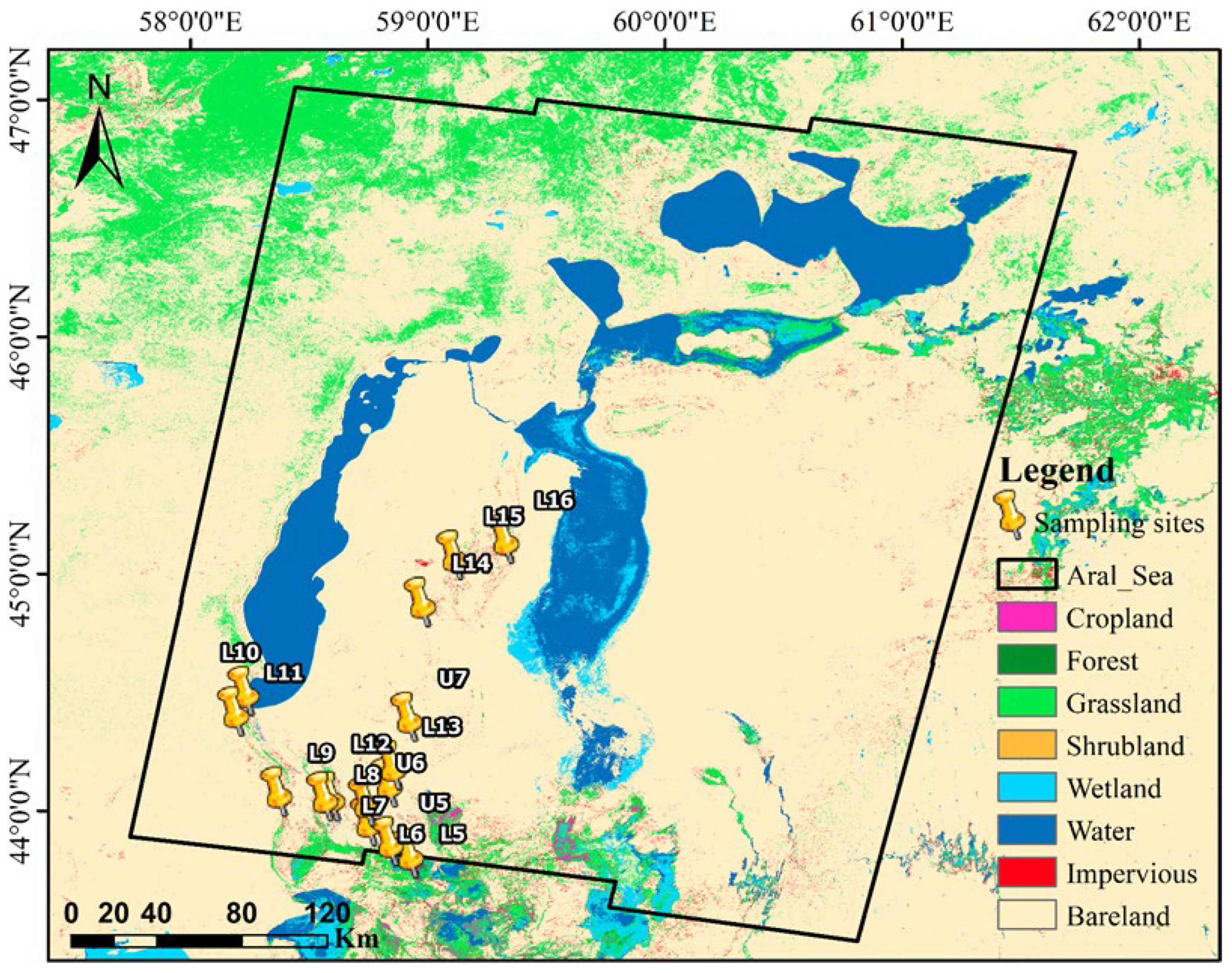
In the Aral Sea, the maximum temperature difference
between spring and summer can reach 60 °C, and the average annual precipitation
is about 100mm, which is very rare. The significant temperature difference and
scarce rainfall are very conducive to wind erosion. The significant temperature
difference and scarce rainfall are very conducive to wind erosion. Furthermore,
as shown in Figure 1, this area is
dominated by bare land. Besides, the desertification of the dry lakebed is
badly severe, and the loose soil is vulnerable to erosion. Thus, the dry
climate, sparse vegetation coverage, and loose soil properties make this area a
potential wind erosion area. Sampling data was from a field survey about the
Aral Sea’s desertification in November 2018, and parts of the sampling sites
are listed in Figure 1.
3. Method and Data
3.1. Soil Sampling and Volumetric Soil Moisture Data
We obtained soil data at the sampling point in this
field survey, including soil photos and soil salinity data. The landscape
photos can visually indicate whether the soil is vulnerable to wind erosion.
Therefore, we can use these data to qualitatively assess the ITDDM model and
the estimation results of SITD. The volumetric soil moisture (topsoil from 0 to
7 cm) data comes from the EAR5 data set on the Google Earth Engine platform and
will be used to extract potential dust emission areas.
3.2. Vegetation Fraction Coverage Data
Vegetation fraction coverage (VFC) is related to
the vegetation and soil’s backscattering weights under the assumption that only
these two land types are in this resolution unit [34].
We can use VFC to estimate the soil microwave backscattring coefficient (SMBC)
and soil microwave backscattring coefficient (VMBC) related to the ITD weights
of vegetation and soil. In this paper, we used NDVI of Landsat 8 to compute VFC
based on the Pixel dichotomy [35], and the
spatial resolution of NDVI data was 30 m.
3.3. Microwave Backscattering Data
Sentinel-1 dataset C-band Synthetic Aperture Radar
(SAR) dataset will be used to estimate SMBC of VMBC of a resolution unit. The
spatial resolution of this data is about 10 m. Usually, the normalized
microwave backscattring coefficient (NMBC) is between 0 and 1. The NMBC and the
microwave backscattring coefficient (MBC) described in dB have a relationship
like this [28]:
Where denotes the MBC in dB, and is NMBC. Due to the very sparse vegetation
coverage in the arid and semi-arid area, the volume scattering is very weak,
and thus we use the ITD of VV polarization to characterize wind erosion of
topsoil. The ITD weights of vegetation and soil are related to the SMBC and
VMBC in the resolution unit. Therefore, the SMBC and VMBC in a resolution unit
will be estimated firstly by the VFC and the total MBC. The backscattering
images with VV polarization taken on June 23, 2020, and July 05, 2020
(https://code.earthengine.google.com/), were obtained, and this time interval
is the same as that for calculating the VFC.
3.4. Soil Sampling Data
We used the Sentinel-1A satellite C-band single
look complex (SLC) SAR images to calculate the ITD of a resolution unit. In
this study, the satellite mode was right-looking, and the orbit cycle was 12
days. We acquired two SLC image pairs with a descending strip-map pattern on
June 23, 2020, and July 05, 2020. The incident angle was about 34.23°, and the
spatial resolution was 20 m after multi look processing. Other information of
two SLC image pairs is shown in Table 1.

Table 1.
Information and interferometry pattern of two SLC image pairs.
| Footprint | Acquisition date | Obit number | Combination mode | Time baseline | Normal baseline |
|---|---|---|---|---|---|
| North Aral Sea | 2020/06/23 | 33138 | master | 12 days | -33.064 m |
| 2020/07/05 | 33313 | slaver | |||
| Aral Sea South | 2020/06/23 | 33138 | master | 12 days | -35.154 m |
| 2020/07/05 | 33313 | slave |
* The Sentinel-1A data is from the copernicus dataspace (https://dataspace.copernicus.eu/).
As is shown in Table. 1, the SLC images acquired on June 23, 2020, were set as the master images, and the others were set as slave images. The absolute time baseline of these two SLC image pairs is 12 days, and the normal baseline is about -33.064 m and -33.154 m for the SLC image pairs of the study area, respectively. The relatively short time baseline setup mainly meets the assumption of identical backscattering levels for acquisitions 1 and 2 [28]. The short spatial baseline is much smaller than the critical baseline, indicating that the influence of the spatial baseline on ITD is negligible [26].
3.5. Method
3.5.1. Wind Erosion Intensity Modeling
Generally, the areas where wind erosion occurs within a resolution unit are randomly distributed. Therefore, the degree of wind erosion of the 1 - D soil profile can help us analyze and define a resolution unit’s degree of wind erosion. Figure 2 shows the deformation of the soil surface in the resolution unit after wind erosion.
The ground surface will sink slightly and randomly after wind erosion for most arid bare lands, except for desert regions. Due to particles’ deposition or surface movement, the ground surface may slightly uplift after wind erosion in desert areas. Fortunately, there are few active deserts in the study area. The deformation of different positions in the resolution unit can be regarded as a random signal at the point . Since the root mean square can describe the intensity of the random signal, we can use the root mean square of the erosion depth at different locations within the resolution unit to define the WEI.
In order to simplify this process, we only consider the discrete case. Assuming that there are N differential elements in a resolution unit, the wind erosion intensity of the resolution unit can be simplified as:
3.5.2. InSAR Temporal Decorrelation
Coherence is used to measure the similarity of the InSAR echoes and is often used to describe different degrees of terrain changes. The coherence between two complex echo signals ( and ) is defined as their correlation coefficient .
Decorrelation , which is equal to , is usually caused by thermal decorrelation , spatial decorrelation , and the temporal decorrelation . Temporal decorrelation due to environmental changes over time can be described by the following formula [26].
3.5.3. The Ralationship between InSAR Temporal Decorrelation and Wind Erosion Intensity
According to the microwave backscattering theory, the differential element’s random subsidence in the resolution unit can be equivalent to the random displacement of the scatterers (or scattering differential bins) in the vertical direction (Figure 3).
Zebker derived the relationship between the root mean square (RMS) displacement of scatterers and ITD [26]:
Where is the ITD for scatterers within a resolution unit, denotes the horizontal displacement of the scatterer, denotes the vertical displacement of the scatterer, and is the incident angle. Since wind erosion in a resolution unit can be equivalent to the vertical displacement of the scatterers within the resolution unit, Equation (5) can be simplified to:
However, it must be noted that the vertical displacement of the scatterers may be positive or negative because of the existence of horizontal displacement of the scatterers or the deposition of the soil particles. In fact, except for the more mobile deserts, most of the bare land in the Aral Sea exhibited random subsidence rather than uplift under wind erosion. Furthermore, the ground uplift caused by the particles’ horizontal displacement and the particles’ deposition is so tiny that it can be ignored. We plotted the relationship between the ITD of the C-band and the wind erosion intensity when the incident angle was 34°, and the results are shown in Figure 4.
According to Figure 4 and formula (6), ITD and WEI have a non-linear negative correlation, which coincides well with Wegmuller’s field survey [28]. However, in bare land of the Aral Sea, a resolution unit usually contains soil and vegetation. Therefore, we must decompose these contributions and estimate the SITD, which can be used to describe the wind erosion degree of soils.
3.5.4. InSAR temporal Decorrelation Decomposition Model
Usually, there is sparse vegetation on the arid bare lands. According to Wegmuller, the ITD of a resolution unit can be decomposed into the contributions of soil and vegetation when there is only soil and vegetation within it [28].
, , and are the VMBC, SMBC and total MBC of this resolution unit, respectively. , and denote the SITD, vegetation ITD (VITD) and total ITD of this resolution unit, respectively. However, before formula 7 can be used to estimate the SITD, we must know the backscattering coefficient of soils and vegetation of a resolution unit. Therefore, a backscattering contribution decomposition (MBCD) model within a resolution unit proposed in our previous work will be used to unmix the backscattering contributions of vegetation and soil and estimate the VMBC and SMBC within a resolution unit [34].
3.5.5. Backscattering Contribution Decomposition and Estimation Within a Resolution Unit
In our previous work about the backscattering contribution decomposition within a resolution unit, we have reached an important conclusion: the SMBC, VMBC, and total MBC of a resolution unit satisfy a simple linear relationship. This relationship can be expressed as [34]:
, and are the VMBC, SMBC and total MBC of a resolution unit, respectively. is the VFC of this resolution unit. Our previous work also provided the estimation method of VMBC and SMBC, which will be used to estimate the SITD [34].
3.5.6. SITD Estimation Based on LSM-SVD Method
The continuity of the spatial distribution of soil and vegetation allows them to have nearly the same temporal decorrelation in adjacent resolution units. Thus, the temporal decorrelation of a resolution unit can be estimated by the sample points within the buffer of this resolution unit. If n sample points around the resolution unit (resolution P) were used to estimate the ITD of vegetation and soil of this resolution unit, n linear equations can be written as:
Where and are the ITD weights of vegetation and soil of the sampling point, and denote VITD and SITD of the resolution unit P, respectively, and is the composite ITD of the sampling point. The system equations (formula (9)) can also be written in the form of a matrix:
Let be the ITD weight matrix, be the InSAR temporal decorrelation decomposition matrix of the resolution unit P, be the InSAR temporal decorrelation composite matrix, and make the following conventions:
Then formula (9) can be can be simplified as:
Then the least squares estimation of can be expressed as:
Considering the huge computational load, we can use the SVD method to estimate SITD. Assume that can be decomposed as follows:
The SVD-based least square estimation of can be expressed as:
When the first singular value of is greater than or equal to 90% of the sum of all its singular values, the value of is 1, and has the following form:
Where is the first singular value of . Otherwise, S has the following form:
Where is the second singular value of .
4. Results
4.1. VFC and MBC of the Study Area
The VFC with a resolution of 30 m calculated by Landsat 8 NDVI and the Sentinel-1A C-band microwave backscattering coefficient of VV polarization with a resolution of 10 m from the Google Earth Engine platform were used to estimate the VMBC and SMBC. To evaluate the vegetation’s influence on the SITD estimation, we also calculated the SMBC to VMBC (SDV) ratio. Suppose the total ITD of the resolution unit replaces the SITD of a resolution unit. In that case, the error mainly depends on the VMBC and SMBC in the resolution unit. The VFC, total MBC, SMBC, VMBC, and SDV are shown in Figure 5. As shown in Figure 5(a), Vegetation coverage in the Aral Sea and its surrounding areas is very sparse. The vegetation coverage of most of the study areas is between 0 and 0.1608. In comparison, the vegetation coverage is relatively high in the northwest and northeast (VFC ranges from 0.1608 to 0.3137) and the southern part of the study area (VFC is between 0.3137 and 1).
It can be seen from Figure 5(b) that, except for the area around the east branch of the South Aral Sea, the backscattering coefficients in other regions are relatively low. Figure 5(c) shows that the soil’s backscattering coefficient is very close to the total backscattering coefficient of the resolution unit. However, there are obvious errors in estimating soil backscattering coefficients in the northwest and northeast of the study area, most probably due to the uniform spatial distribution of vegetation [34]. In addition, the results of backscattering coefficient estimation have been fully verified in our previous work, so this paper will not refer to the verification of backscattering coefficient estimation results [34]. Furthermore, the areas with incorrect backscattering coefficient estimation results often have relatively high soil water content or vegetation coverage, so we can remove these places from the study area, which will be discussed in Section 4.2. Figure 5(c) shows that the backscattering coefficient of soil is much higher for most of the study area than that of vegetation. According to formula (10) and SDV shown in Figure 5, the influence of vegetation on SITD in the resolution unit may be negligible. However, when the SMBC in a resolution unit is close to the VMBC (such as in severely desertified areas), the ITD weights of vegetation and soil are almost the same. In this case, the impact of vegetation on SITD is not negligible. The process of MBC and ITD estimation is badly time-consuming. Extracting the potential wind erosion area can significantly reduce the target area and effectively reduce the amount of calculation. Numerous studies have shown that wind erosion is almost impossible in these areas when the soil moisture exceeds 10%, or the VFC is higher than 40% [36,37,38,39,40,41,42]. When the vegetation coverage exceeds 40%, the volumetric soil moisture is usually higher than 10%. Our survey results also show that when the vegetation coverage exceeds 40%, the soil volumetric water content is usually higher than 10% [34]. Therefore, these areas can be removed from the study area to reduce the amount of calculation effectively. In the following section, we obtained soil moisture data. Soil moisture and vegetation coverage data were used to extract potential wind erosion areas.
4.2. Potential Wind Erosion Areas
We used GIS software to label the areas with vegetation coverage higher than 0.4 or volumetric soil moisture higher than 0.1 in the study area. Then we got the potential wind erosion area, and the result is shown in Figure 6. It should be noted that since the volumetric soil moisture (VSM) of only one pixel in area B exceeds 10%, we have ignored this area. Figure 6 shows that except for areas B, E, and F, the rest of the lakebed is vulnerable to wind erosion.
4.3. InSAR Temporal Decorrelation of Soil
We calculated the SITD of all regions except regions A, B, D, E, and F based on Equation 15. The process of SITD estimation was like that of MBC. The upper and lower thresholds of the VFC difference are set to 0.2 and 0.05, respectively, and the buffer size is set to 100 meters in this paper. Even so, the calculation process is still quite time-consuming. Therefore, we resample the ITD weights of soil and vegetation and the total ITD to 50 meters to further reduce the amount of calculation. The estimated result of SITD is shown in Figure 7. Figure 7 shows that the areas with severe temporal decorrelation are mainly distributed in the bare lands of the middle, northeast, and southeast of the South Aral Sea. In addition, the coastal areas of the North Aral Sea are also areas with severe soil InSAR temporal decorrelation. Beyond the boundaries of the water body of the Aral Sea in 1973, the soil InSAR temporal decorrelation in most areas is very slight. This significant contrast indicates that the dry lakebed is highly susceptible to wind erosion.
The pixel-scale SITD and the corresponding landscape photos are shown in Figure 8.
The landscape photos in Figure 8 clearly show the soil’s actual condition near the sampling points, which can be used to visually judge the degree of soil susceptibility to wind erosion. The SITD will be used to describe the spatial distribution of wind erosion of different degrees. Like the description in part 3.3, because the waters and wetland cannot be the potential place where wind erosion will happen, the SITD was not be estimated for these two land types. In the next section, SITD will be used to describe the WEI of the study area.
4.4. Wind Erosion at the Dry Bottom of the Aral Sea
Do an inverse transform to Equation (6), and then we can convert SITD to WEI. Furthermore, we divided WEI into eight levels, and the results are shown in Figure 9. Figure 9 shows that the wind erosion in the study area mainly occurs on the lakebed. Besides, our previous field survey showed that the dry lakebed is rich in salt and toxic substances [34]. Therefore, the fine particles produced in the wind erosion process should also be rich in these materials.
Salt storms that carry fine particles rich in salt and toxic substances will badly threaten the surrounding ecosystems and human health. Therefore, we simply count the wind erosion area of the dry lakebed. We used GIS software to remove areas with VFC greater than or equal to 4, areas with VSM greater than or equal to 0.1, wetlands, and water bodies from the Aral Sea water surface in 1973. Then, we used this vector to extract the WEI map of the potential wind erosion area on the dry bottom of the Aral Sea. At last, we performed simple statistics on the wind erosion intensity, and the results are shown in Table 2.
5. Discussion
Due to the harsh natural environmental conditions of the Aral Sea, it is a challenge to verify the accuracy of dust activity intensity described by soil temporal decorrelation through the measurement of dust activity intensity. The sampling data for validation is from a joint desertification survey referring to the Aral Sea in 2018 by China and Uzbekistan. However, the survey was not designed specifically for this research, so we can only provide limited validation by analyzing the partial sampling data. Nevertheless, through rigorous theoretical derivation, little sampling points, and supporting literature, we can still prove the accuracy of the spatiotemporal distribution results of dust activity intensity described in this paper. The accuracy of the spatiotemporal distribution results of dust activity intensity in the Aral Sea depends on three aspects:
1. Can soil temporal decorrelation accurately describe dust activity intensity?
2. Whether soil temporal decorrelation only depends on the mathematical expectation of phase random variation within the resolution unit and whether other factors, such as variation of soil dielectric constant and soil roughness, will affect soil temporal decorrelation.
3. Are the estimation results of soil temporal decorrelation accurate?
For the first question, we have provided a comprehensive argumentation through the proposal of dust activity intensity in Section 3.5.2 and the derivation of the relationship between dust activity intensity and soil temporal decorrelation in Section 3.5.3, which demonstrates the feasibility of using soil temporal decorrelation to describe dust activity intensity. Next, we will discuss the impact of the other two factors.
5.1. The Impact of Non-Phase Factors on Soil Temporal Decorrelation
According to the definition of soil temporal decorrelation, it mainly depends on the variations in the backscattering coefficient and phase during the interferometric period. Significant changes in soil roughness, moisture content, and salinity can all lead to notable variations in backscattering levels. Through an investigation of precipitation during the interferometric period, no significant rainfall was observed in these regions within 1-2 days before the second imaging (in June and July, the temperature in the Aral Sea is high, and any small amount of rainfall occurring a few days before the second imaging would quickly evaporate). This survey indicates that the soil moisture content in most areas is unlikely to undergo significant changes, thus not significantly influencing the backscattering coefficient. The soil salinity of the Aral Sea primarily comes from the evaporated seawater, and after the seawater dries up, the salt deposits in the soil at the bottom of the dried-up lake. Therefore, the soil salinity is unlikely to undergo significant changes over a relatively short time interval (12 days), and thus, it cannot cause drastic variations in the backscattering coefficient. The spatial continuity of soil types within the resolution unit and similar wind conditions within the unit ensure slight variation in erosion levels among different regions within the unit. Consequently, the surface roughness variation is relatively minor. Therefore, the soil temporal decorrelation of a resolution unit primarily depends on the mathematical expectation of phase random variations at different locations within this resolution unit, representing dust activity intensity, and these phase variations are mainly caused by wind erosion.
5.2. The Results of SITD Estimation Assessment
The accuracy of soil temporal decorrelation estimation primarily depends on the assumptions made during the decomposition and estimation. According to Wegmuller’s research, two assumptions regarding the soil temporal decorrelation decomposition model are often valid for bare soil and sparse low vegetation regions in arid and semi-arid areas. The estimation was based on the assumption that "spatial adjacent resolution units have the same soil and vegetation temporal decorrelation." Soil and vegetation’s temporal decorrelation primarily depend on all scatterers’ root mean square displacement within a resolution unit. Spatial adjacent resolution units have similar vegetation types and structures, soil types and structures, and highly similar wind conditions. Therefore, the root mean square of soil random erosion of a resolution unit is almost the same as that of an adjacent resolution unit. Similarly, a resolution unit’s vegetation temporal decorrelation is nearly the same as that of an adjoining resolution unit. Hence, the assumption that a resolution unit’s soil or vegetation temporal decorrelation is almost the same as that of a spatial adjacent resolution unit is reasonable.
The differences in the backscattering coefficients of soil and vegetation among adjacent resolution units are the prerequisite for estimating the soil and vegetation temporal decorrelation. Because of the slight differences in soil dielectric constant (due to spatial variations in soil moisture and salinity), soil roughness (due to the spatial difference of wind erosion depth within a resolution units), vegetation dielectric constant (due to spatial variations in vegetation moisture content, vegetation type, vegetation density, health, and condition), and vegetation roughness (due to the spatial distribution variations in leaf structure, branching patterns, vegetation canopy height and density, vegetation growth stage, and environmental factors.), the backscattering coefficients of soil and vegetation in adjacent resolution units often exhibit differences. Consequently, it is possible to accurately estimate the soil temporal decorrelation of a resolution unit.
As described in Section 4.3, we use the SITD maps (SITDMs) and the corresponding landscape photos to verify the estimation results of SITD. As is shown in landscape photos of L5, L6 and L15, some parts of arid soil are covered by relatively dense vegetation, while some are covered by very sparse vegetation. Besides, these two landscape photos also showed that the soil is relatively loose here. According to the study of Bagnold, the ground surface wind speed will significantly decrease when the vegetation exists, and the degree of wind erosion will also be declined [4]. So, the wind erosion of soils around L5, L6 and L15 with few vegetation coverages is severe but is relatively slight for soils around L5, L6 and L15 with relatively dense vegetation coverage, and the wind erosion of soils shown in SITDMs coincides well with the actual soil property shown in the corresponding landscape photos. Although there is few vegetation at site L7, the soil was very stable according to the ITDM of L7. Precipitation around L7 between June 22, 2020, and July 05, 2020, is a possible cause of the stable status of soils. The relatively stable status of L8, L9 and L11 shown in their corresponding SITDMs is most probably the result of dense vegetation coverage showed in their corresponding landscape photos. The relatively slight wind erosion of L10 (SITDM of L10) may be due to soil’s high-water content, which is most probably the result of the short distance between L10 and water. As shown in the landscape photos of site L12, the desertification trend is severe. However, the SITDM of L12 indicates the soil here is very stable, and the relatively stable status of the soil is most probably due to the rain between June 23, 2020, and July 05, 2020, which can reduce the wind erosion significantly [33]. In Figure 8, the soil property of L13 is just the same as that of L12, and the corresponding SITDM indicates the wind erosion here is very severe, so the actual soil property shown in the landscape photo is also in good agreement with the wind erosion degree shown in the corresponding SITDM. The landscape photos of L14 and U7 shows that there is few vegetation at these places, but this place is rich in relatively large stones. The large stones are hard to be moved by wind, and meanwhile, they can reduce the wind speed on the ground surface, which made this place remarkably stable. For L16, as is shown in the landscape photos of L16, there are many artificial buildings and roads here, the SITD and backscattering coefficient of which are much higher than that of vegetation [32]. Therefore, the SITD should be very high for the resolution unit with buildings in it according to formula (10). The high SITD of L16 showed in its SITDM coincides nicely with the soil property shown in the landscape photo of L16. Large areas of bare soil were found around U5 and U6, and there are few large stones here, so U5 and U6 are very vulnerable to soil erosion. The analysis above is consistent with the severity of wind erosion shown in the SITDMs of U5 and U6. In conclusion, the SITDMs, except for some influenced by precipitation, are all consistent with the actual soil property shown in the corresponding landscape photos, and this result indicates that SITD can be used to describe the severity of wind erosion.
The 2008 NOAA AVHRR images (Figure 10) show that the dust emission areas are mainly distributed in the bare land between the two branches of the South Aral Sea, the northeast and southeast of the South Aral Sea [43]. These areas spatially coincide well with the results of this study.
Besides, investigation regarding the dust storm events in the Aral Sea (2005-2008) also indicates that the northeastern and southeastern parts of the South Aral Sea are the right places where dust storms often occur [43]. Although sandstorm events also happened in the bare land between the two branches of the South Aral Sea, the frequency is much lower than that of the northeast and southeast of the South Aral Sea. Therefore, the locations of dust emission identified in this study, except for the bare land between the two branches of the South Aral Sea, are consistent with the investigation results. A plausible explanation is that desertification had already occurred in the bare land between the two branches of the South Aral Sea in 2008 or even before, but the desertification was mild. After about 12 years of desertification, this region’s desertification becomes severe.
Furthermore, the dust activity intensity of this region described in this paper is confirmed by the landscape photographs of the three sampling points falling in this area (Figure 11). Therefore, it is highly likely that the bare land between the two branches of the South Aral Sea has developed into a new outbreak area for salt and dust storms.
5.3. Wind Erosion at the Dry Bottom of the Aral Sea
(1) Overview of the wind erosion in the Aral Sea
We conducted a simple statistic of different degrees of the WEI according to Figure 9, and the results showed that the dry lakebed is suffering from different degrees of wind erosion. The area with wind erosion intensity greater than 1.5 cm accounts for 0.2790% of the lakebed, which is about 176 square kilometers. The area with wind erosion intensity ranging from 1 to 1.5 cm accounts for 2.2560%, approximately 1,426 square kilometers. The site with a wind erosion intensity of 0.5 to 1 cm accounts for 35.5420%, approximately 22,471 square kilometers. The area with a wind erosion intensity of 0.4 to 0.5 cm accounts for 15.3211%, approximately 9,687 square kilometers. The site with wind erosion intensity between 0.3 and 0.4 cm accounts for 15.4784%, about 9,786 square kilometers. The area with a wind erosion intensity of 0.2 to 0.3 cm accounts for 27.2261%, approximately 17,214 square kilometers. The site with wind erosion intensity ranging from 0.1 to 0.2 cm accounts for 3.723%, about 2,354 square kilometers. The area with wind erosion intensity between 0 and 0.1 cm occupies 0.1736%, approximately 110 square kilometers.
(2) Spatial distribution of wind erosion
According to the WEI of the study area, the severe wind erosion areas () are mainly distributed in bare lands of the middle, the northeast, and southeast of the South Aral Sea. The spatial distribution of the moderate wind erosion area () is the same as that of the severe wind erosion area. The moderate and the severe wind erosion area coincide well with the area of sand and dust activities, and these areas can be treated as the focus areas for people to intervene in sand and dust activities [43]. The severe wind erosion areas within the dry lakebed are the most probably where salt dust storms occur.
5. Conclusions
For areas where desertification is not severe, since the backscattering coefficient of rough topsoil is much higher than that of vegetation, the ITD weight of the soil is far higher than that of the vegetation. Therefore, in these areas, the soil ITD can be approximately replaced by the total ITD of the resolution unit. However, for areas with desertification, the backscattering coefficient of smooth topsoil is very close to the backscattering coefficient of vegetation, so the ITD weights of soil and vegetation should also be very close to each other. In this case, the influence of vegetation on SITD cannot be ignored. The consistency between the SITDM of the sampling points and the actual soil property shown in the corresponding landscape photos indicates that ITDDM and the corresponding estimation method can accurately estimate the SITD in the resolution unit. The wind erosion areas are mainly distributed in bare lands of the middle, the northeast, and southeast of the South Aral Sea. The severe wind erosion areas within the range of the dry lakebed are the most possible places where salt dust storms occur.
Author Contributions
Conceptualization, H.Z. and Y.S.; methodology, Y.S.; software, Q.G.; validation, Y.S., H.Z. and X.X.; formal analysis, G.L.; investigation, W.X.; resources, H.Z.; data curation, O.H.; writing—original draft preparation, Y.S.; writing—review and editing, H.Z.; visualization, T.L.; supervision, A.B.; project administration, J.L.; funding acquisition, H.Z. All authors have read and agreed to the published version of the manuscript.
Funding
This work was supported by the National Natural Science Foundation of China (E0130105 and 42230708), the Tianshan Talent Training Program of Xinjiang Uygur Autonomous region (2022TSYCLJ0011), the Key R&D Program of Xinjiang Uygur Autonomous Region (2022B03021, 2022B03001), the High-End Foreign Experts Project (2020-2023, G2023046005L), the West Light Foundation of The Chinese Academy of Sciences (No. 2020-XBQNXZ-009), the Science and Technology Project of Hebei Education Department (Grant No. QN2020429), the Deprtment of Education, Hebei Province (ZD2022089), The grant from the Deprtment of Education, North China Institute of Aerospace Engineering (BKY-2023-03), the Youth Fund project of the Department of Education of Hebei province, (Grant No. QN2022076), the Science and Technology Project of Hebei Education Department (Grant No. QN2024113), and the central government guides local science and technology development fund projects (Grant No. 216Z0303G).
Data Availability Statement
The data used in this article can be obtained from the Google Earth Engine cloud platform (https://earthengine.google.com/) and the European Space Agency website (https://dataspace.copernicus.eu/), and the relevant code can be obtained from the corresponding author.
Acknowledgments
Thanks to Professor Dong Xiaolong from the National Space Science Center of the Chinese Academy of Sciences for his help in the derivation of the ITDDM model.
Conflicts of Interest
The authors declare no conflicts of interest.
References
- Micklin, P. The Aral Sea disaster. In Annual Review of Earth and Planetary Sciences; Annual Review of Earth and Planetary Sciences; 2007; Volume 35, pp. 47-72.
- Kok, J.F.; Parteli, E.J.R.; Michaels, T.I.; Karam, D.B. The physics of wind-blown sand and dust. Reports on Progress in Physics 2012, 75. [Google Scholar] [CrossRef] [PubMed]
- Shao, Y. Physics and Modelling of Wind Erosion. In Physics and Modelling of Wind Erosion; Atmospheric and Oceanographic Sciences Library; 2009; Volume 37, pp. 1-452.
- Bagnold, R.A. Sand and Dust. In The Physics of Blown Sand and Desert Dunes; Springer Netherlands: Dordrecht, 1974; pp. 1–9. [Google Scholar]
- Lu, H.; Shao, Y.P. A new model for dust emission by saltation bombardment. Journal of Geophysical Research-Atmospheres 1999, 104, 16827–16841. [Google Scholar] [CrossRef]
- Bagnold, R.A. The Behaviour of Sand Grains in the Air. In The Physics of Blown Sand and Desert Dunes; Springer Netherlands: Dordrecht, 1974; pp. 10–24. [Google Scholar]
- Ungar, J.E.; Haff, P.K. STEADY-STATE SALTATION IN AIR. Sedimentology 1987, 34, 289–299. [Google Scholar] [CrossRef]
- Anderson, R.S.; Sørensen, M.; Willetts, B.B. A review of recent progress in our understanding of aeolian sediment transport. Vienna, 1991; pp. 1-19.
- Ruff, S.W.; Pankine, A.A.; Barta, G. Aeolian Dust Deposits. In Encyclopedia of Planetary Landforms, Hargitai, H., Kereszturi, Á., Eds.; Springer New York: New York, NY, 2015; pp. 12–18. [Google Scholar]
- Rice, M.A.; Willetts, B.B.; McEwan, I.K. Observations of collisions of saltating grains with a granular bed from high-speed cine-film. Sedimentology 1996, 43, 21–31. [Google Scholar] [CrossRef]
- Pye, K.; Tsoar, H. Mechanics of Aeolian Sand Transport. In Aeolian Sand and Sand Dunes; Springer Berlin Heidelberg: Berlin, Heidelberg, 2009; pp. 99–139. [Google Scholar]
- Wang, Z.-T.; Zhang, C.-L.; Wang, H.-T. Forces on a saltating grain in air. European Physical Journal E 2013, 36. [Google Scholar] [CrossRef] [PubMed]
- Owen, P.R. SALTATION OF UNIFORM GRAINS IN AIR. Journal of Fluid Mechanics 1964, 20, 225–242. [Google Scholar] [CrossRef]
- Anderson, R.S.; Haff, P.K. SIMULATION OF EOLIAN SALTATION. Science 1988, 241, 820–823. [Google Scholar] [CrossRef]
- Walter, B.; Horender, S.; Voegeli, C.; Lehning, M. Experimental assessment of Owen’s second hypothesis on surface shear stress induced by a fluid during sediment saltation. Geophysical Research Letters 2014, 41, 6298–6305. [Google Scholar] [CrossRef]
- Malina, F.J. Recent developments in the dynamics of wind erosion. Transactions-American Geophysical Union 1941, 22, 262–287. [Google Scholar]
- Anderson, R.S. THE PATTERN OF GRAINFALL DEPOSITION IN THE LEE OF AEOLIAN DUNES. Sedimentology 1988, 35, 175–188. [Google Scholar] [CrossRef]
- Ning, H.; Yandan, G.U. Review of the Mechanism of Dust Emission and Deposition. Advance in Earth Sciences 2009, 24, 1175–1184. [Google Scholar]
- Chepil, W.S. DYNAMICS OF WIND EROSION.1. NATURE OF MOVEMENT OF SOIL BY WIND. Soil Science 1945, 60, 305–320. [Google Scholar] [CrossRef]
- Woodruff, N.P.; Armbrust, D.V. A MONTHLY CLIMATIC FACTOR FOR WIND EROSION EQUATION. Journal of Soil and Water Conservation 1968, 23, 103-&. [Google Scholar]
- Bocharov, A. A description of devices used in the study of wind erosion of soils; AA Balkema: 1984.
- Singh, U.B.; Gregory, J.M.; Wilson, G.R. Texas erosion analysis model: theory and validation. In Proceedings of the Proceedings of Wind Erosion: An International Symposium/Workshop, 1997; pp. 3–5.
- Shao, Y.P.; Raupach, M.R.; Leys, J.F. A model for predicting aeolian sand drift and dust entrainment on scales from paddock to region. Australian Journal of Soil Research 1996, 34, 309–342. [Google Scholar] [CrossRef]
- Van Pelt, R.S.; Zobeck, T.M.; Potter, K.N.; Stout, J.E.; Popham, T.J.E.M. ; Software. Validation of the wind erosion stochastic simulator (WESS) and the revised wind erosion equation (RWEQ) for single events. 2004, 19, 191–198. [Google Scholar]
- Hagen, L. A wind erosion prediction system to meet user needs. Journal of soil water conservation 1991, 46, 106–111. [Google Scholar]
- Zebker, H.A.; Villasenor, J. DECORRELATION IN INTERFEROMETRIC RADAR ECHOES. Ieee Transactions on Geoscience and Remote Sensing 1992, 30, 950–959. [Google Scholar] [CrossRef]
- Wang, T.; Liao, M.; Perissin, D. InSAR Coherence-Decomposition Analysis. Ieee Geoscience and Remote Sensing Letters 2010, 7, 156–160. [Google Scholar] [CrossRef]
- Wegmuller, U.; Strozzi, T.; Farr, T.; Werner, C.L. Arid land surface characterization with repeat-pass SAR interferometry. Ieee Transactions on Geoscience and Remote Sensing 2000, 38, 776–781. [Google Scholar] [CrossRef]
- Bodart, C.; Ozer, A.J.E.S.A.S.; Reports, T. The use of SAR interferometric coherence images to study sandy desertification in southeast Niger: Preliminary results. 2007, 636.
- Bodart, C.; Gassani, J.; Salmon, M.; Ozer, A. Contribution of SAR interferometry (from ERS1/2) in the study of aeolian transport processes: the cases of Niger, Mauritania and Morocco. In Desertification and risk analysis using high and medium resolution satellite data; Springer: 2009; pp. 129-136.
- Gaber, A.; Abdelkareem, M.; Abdelsadek, I.S.; Koch, M.; El-Baz, F. Using InSAR Coherence for Investigating the Interplay of Fluvial and Aeolian Features in Arid Lands: Implications for Groundwater Potential in Egypt. Remote Sensing 2018, 10. [Google Scholar] [CrossRef]
- Havivi, S.; Amir, D.; Schvartzman, I.; August, Y.; Maman, S.; Rotman, S.R.; Blumberg, D.G. Mapping dune dynamics by InSAR coherence. Earth Surface Processes and Landforms 2018, 43, 1229–1240. [Google Scholar] [CrossRef]
- Song, Y.; Chen, C.; Xu, W.; Zheng, H.; Bao, A.; Lei, J.; Luo, G.; Chen, X.; Zhang, R.; Tan, Z. Mapping the temporal and spatial changes in crescent dunes using an interferometric synthetic aperture radar temporal decorrelation model. Aeolian Research 2020, 46. [Google Scholar] [CrossRef]
- Song, Y.; Zheng, H.; Chen, X.; Bao, A.; Lei, J.; Xu, W.; Luo, G.; Guan, Q. Desertification Extraction Based on a Microwave Backscattering Contribution Decomposition Model at the Dry Bottom of the Aral Sea. 2021, 13, 4850. [Google Scholar] [CrossRef]
- Li, M.; Wu, B.; Yan, C.; Zhou, W. Estimation of Vegetation Fraction in the Upper Basin of Miyun Reservoir by Remote Sensing. Resources science 2004, 26, 153–159. [Google Scholar]
- Chen, W.N.; Dong, Z.B.; Li, Z.S.; Yang, Z.T. Wind tunnel test of the influence of moisture on the erodibility of loessial sandy loam soils by wind. Journal of Arid Environments 1996, 34, 391–402. [Google Scholar] [CrossRef]
- Wang, Y.; Tang, Z.; Chen, C.; Cui, Y.; Wang, J. Wind tunnel experimental study on desert surface of Kubuqi desert, Inner Mongolia. China Environmental Science 2017, 37, 2888–2895. [Google Scholar]
- vanDijk, P.M.; Stroosnijder, L.; deLima, J. The influence of rainfall on transport of beach sand by wind. Earth Surface Processes and Landforms 1996, 21, 341–352. [Google Scholar] [CrossRef]
- Bisal, F.; Hsieh, J. INFLUENCE OF MOISTURE ON ERODIBILITY OF SOIL BY WIND. Soil Science 1966, 102, 143. [Google Scholar] [CrossRef]
- Wolfe, S.A.; Nickling, W.G. THE PROTECTIVE ROLE OF SPARSE VEGETATION IN WIND EROSION. Progress in Physical Geography 1993, 17, 50–68. [Google Scholar] [CrossRef]
- Okin, G.S. A new model of wind erosion in the presence of vegetation. Journal of Geophysical Research-Earth Surface 2008, 113. [Google Scholar] [CrossRef]
- Zhang, C.; Zou, X.; Dong, G.; Liu, Y. Wind Tunnel Studies on Influences of Vegetation on Soil Wind Erosion. Journal of Soil and Water Conservation 2003, 17, 31–33. [Google Scholar]
- Indoitu, R.; Kozhoridze, G.; Batyrbaeva, M.; Vitkovskaya, I.; Orlovsky, N.; Blumberg, D.; Orlovsky, L. Dust emission and environmental changes in the dried bottom of the Aral Sea. Aeolian Research 2015, 17, 101–115. [Google Scholar] [CrossRef]
Figure 2.
Wind erosion at 1–D soil surface.
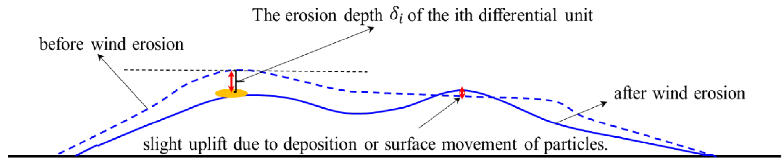
Figure 3.
Wind erosion from the perspective of microwave remote sensing. The displacement of the scatterer in the resolution unit caused by wind erosion can be described by the random variable
Figure 3.
Wind erosion from the perspective of microwave remote sensing. The displacement of the scatterer in the resolution unit caused by wind erosion can be described by the random variable
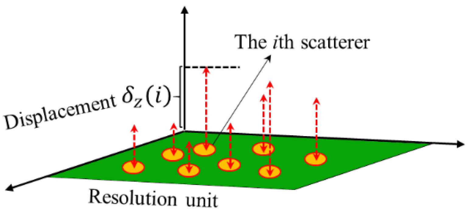
Figure 4.
Relationship between the ITD and WEI.
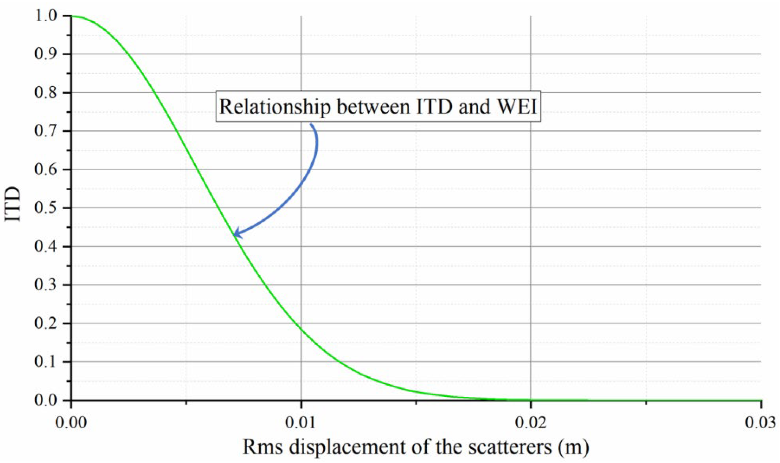
Figure 5.
The VFC, total MBC, SMBC, VMBC, and SDV of the study area. Figure 5(a), Figure 5(b), Figure 5(c), Figure 5(d), and Figure 5(e) are the VFC, total MBC, SMBC, VMBC, and SDV, respectively.
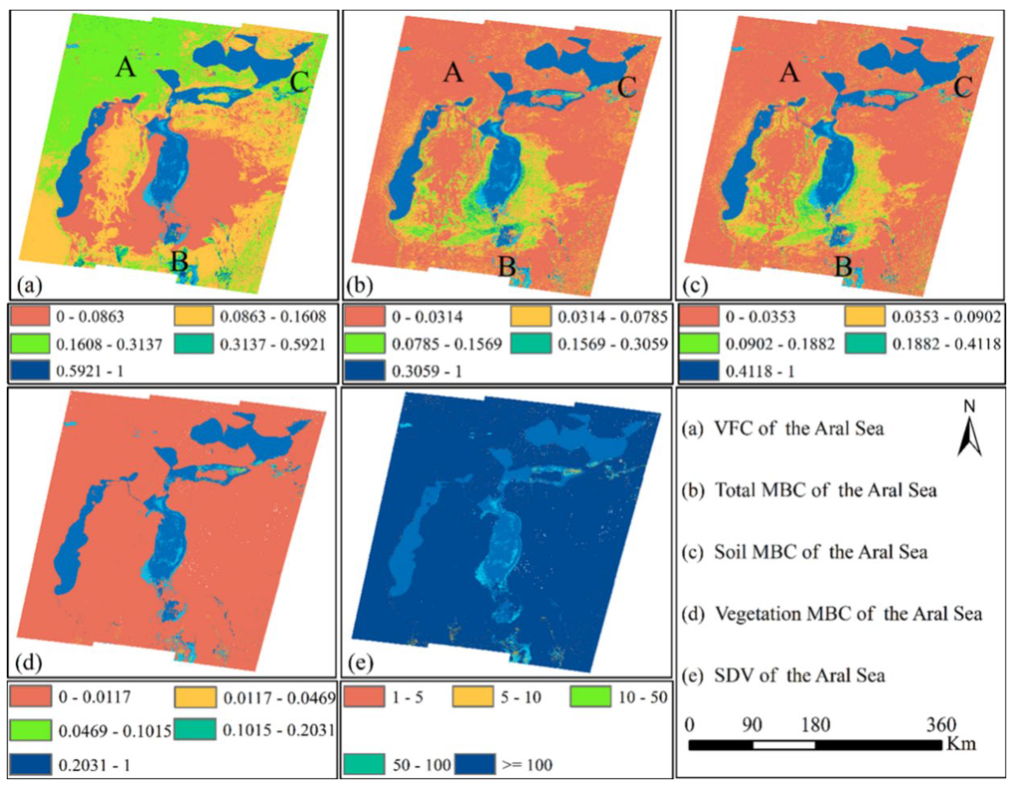
Figure 6.
The potential wind erosion regions in the study area.
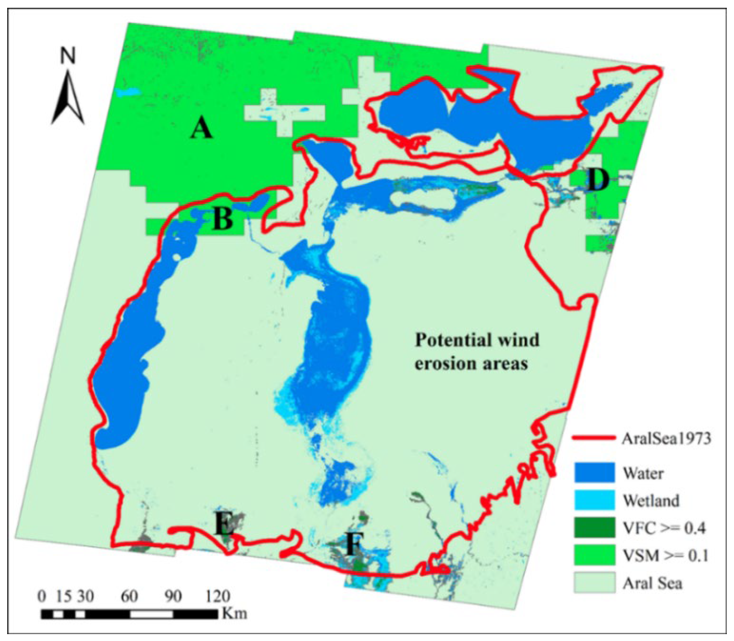
Figure 7.
The SITD map of Aral Sea.
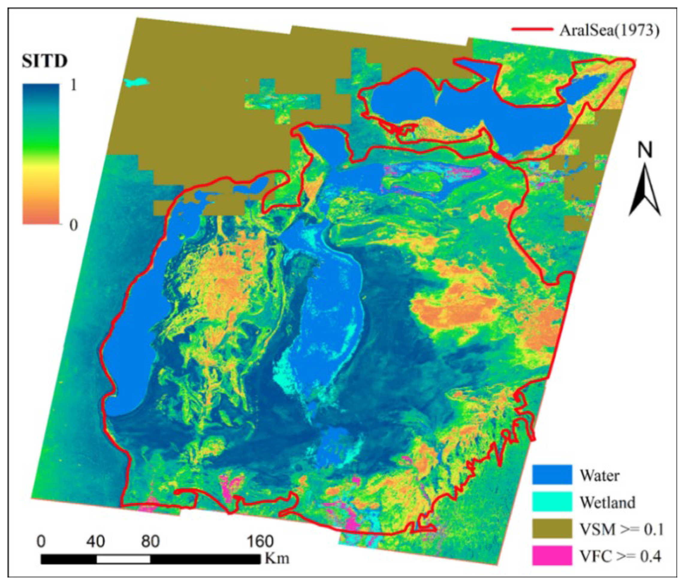
Figure 8.
The results of SITD estimation and their corresponding landscape photos of 15 sampling sites.
Figure 8.
The results of SITD estimation and their corresponding landscape photos of 15 sampling sites.
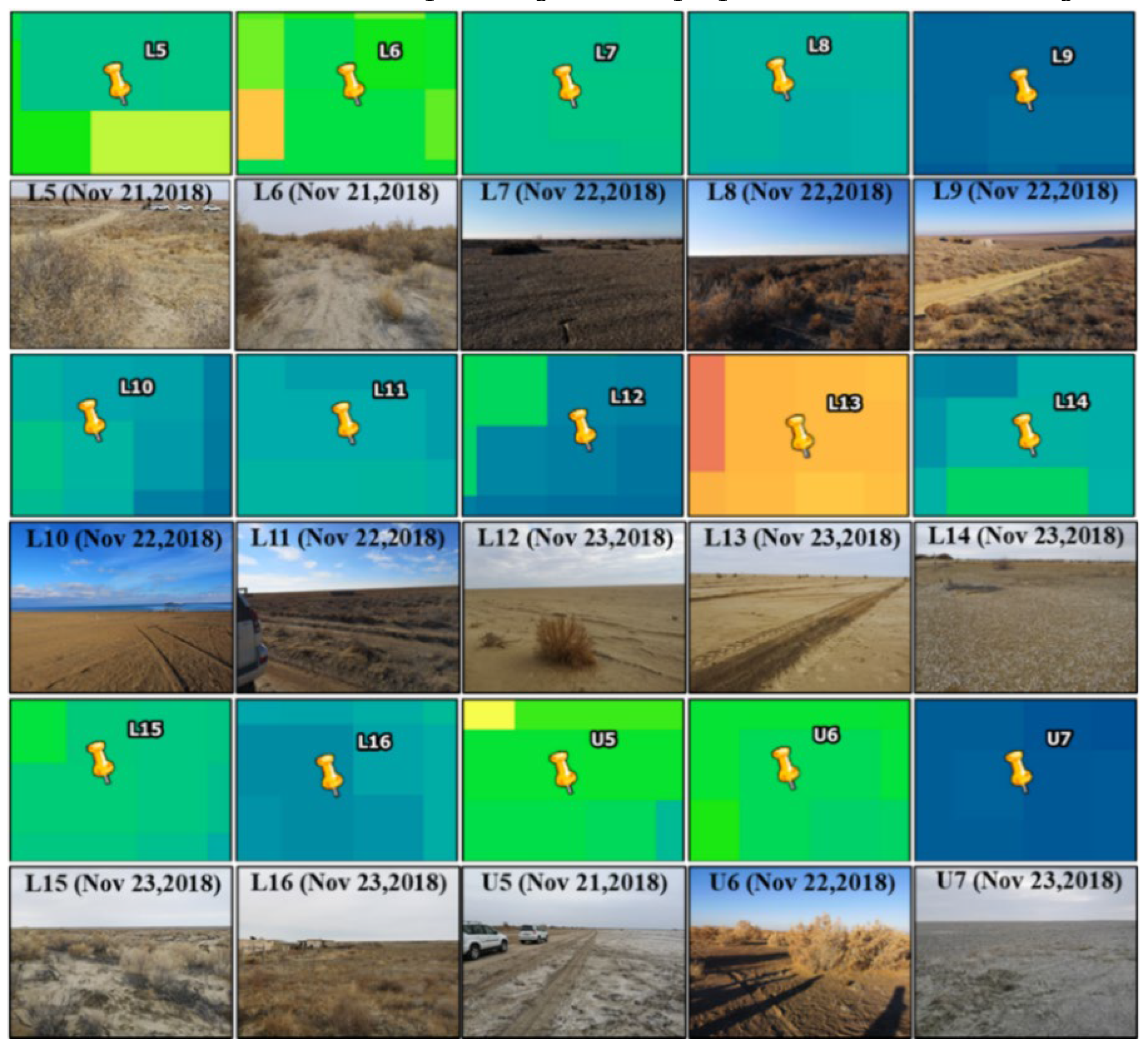
Figure 9.
WEI of the Aral Sea.
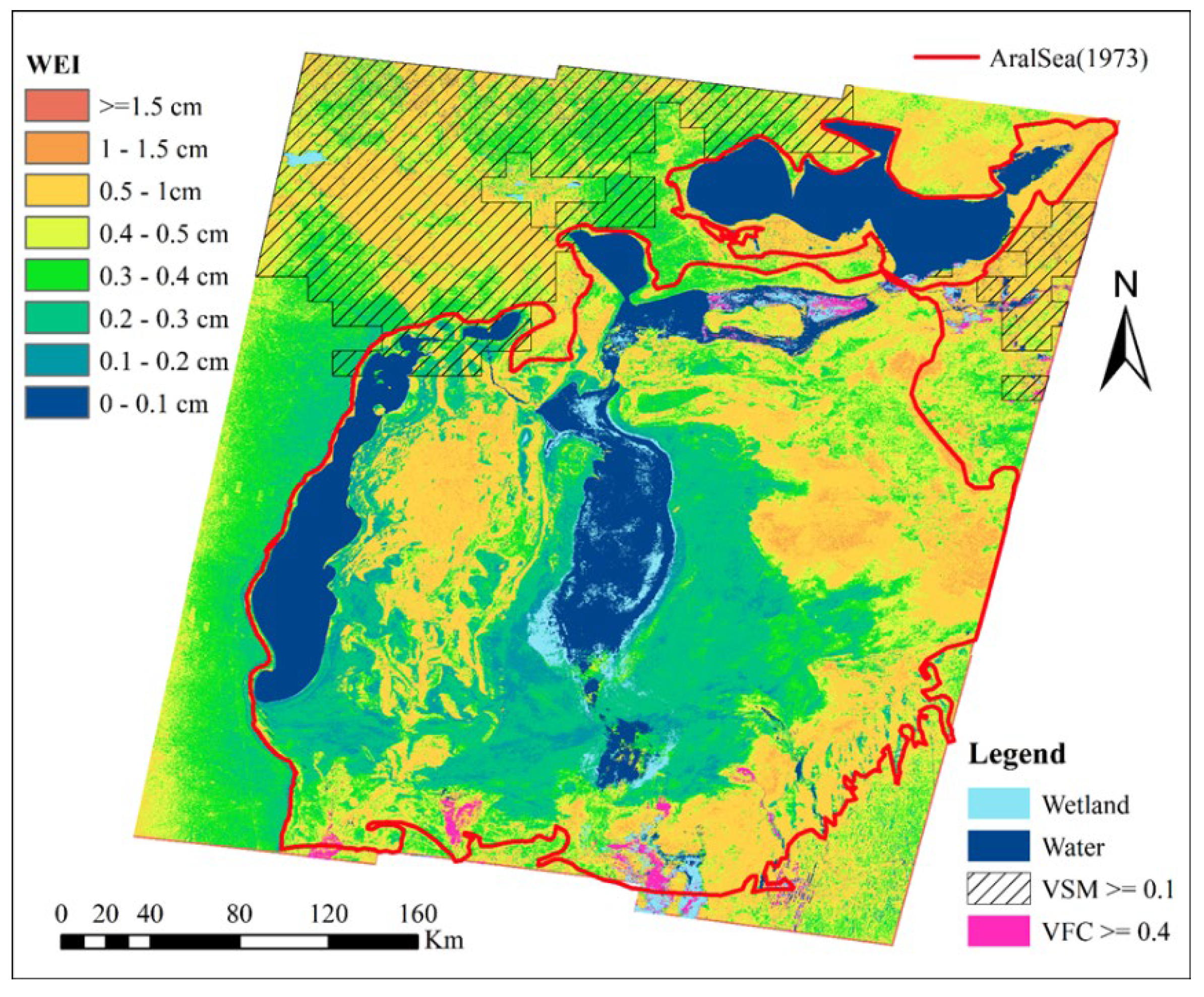
Figure 10.
NOAA-AVHRR images for the dust event from 2005 to 2008 [43].
Figure 10.
NOAA-AVHRR images for the dust event from 2005 to 2008 [43].
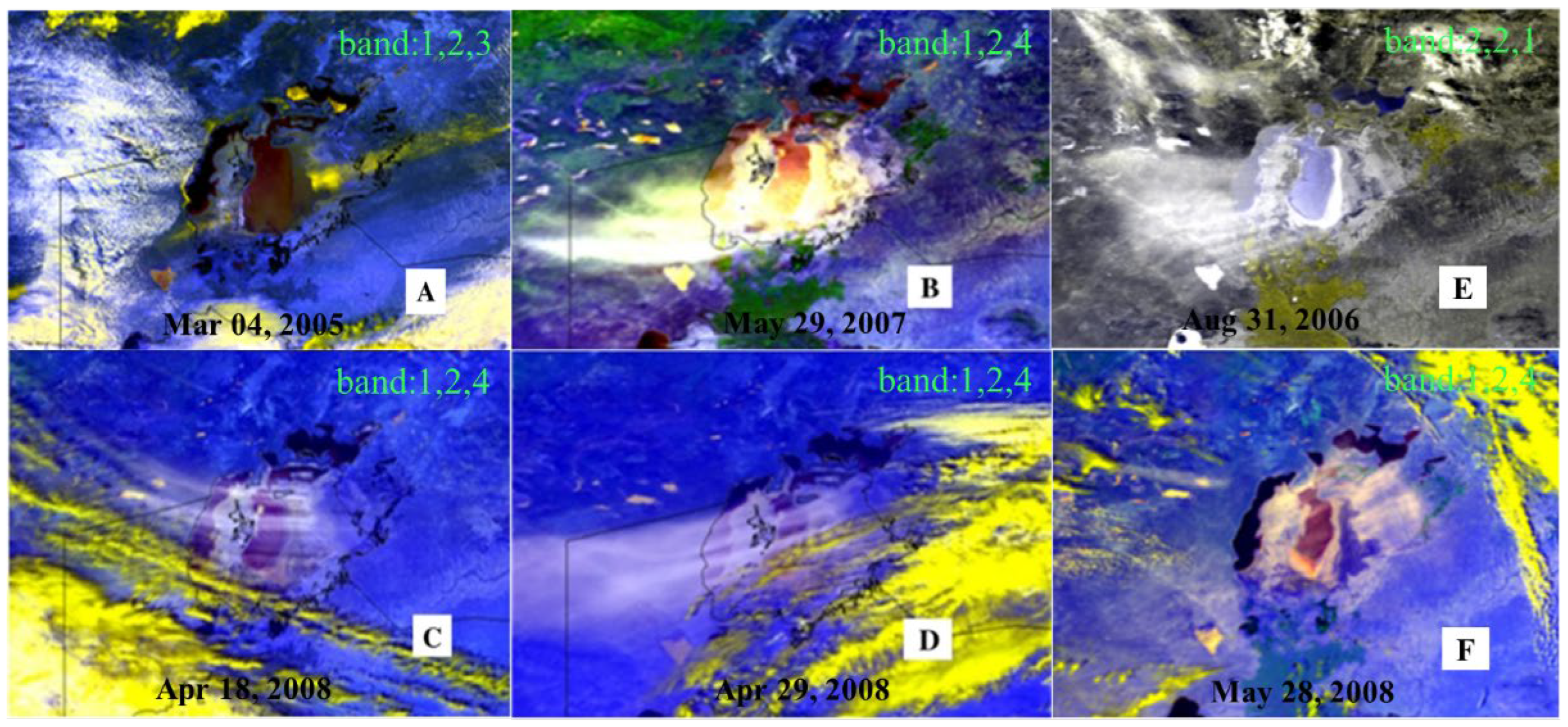
Figure 11.
Soil temporal decorrelation with landscape photos of sampling sites in the bare land between the two branches of the South Aral Sea. The value of soil time decorrelation is between 0 and 1. The smaller the value, the darker the corresponding pixel, and the larger the value, the brighter the corresponding pixel.
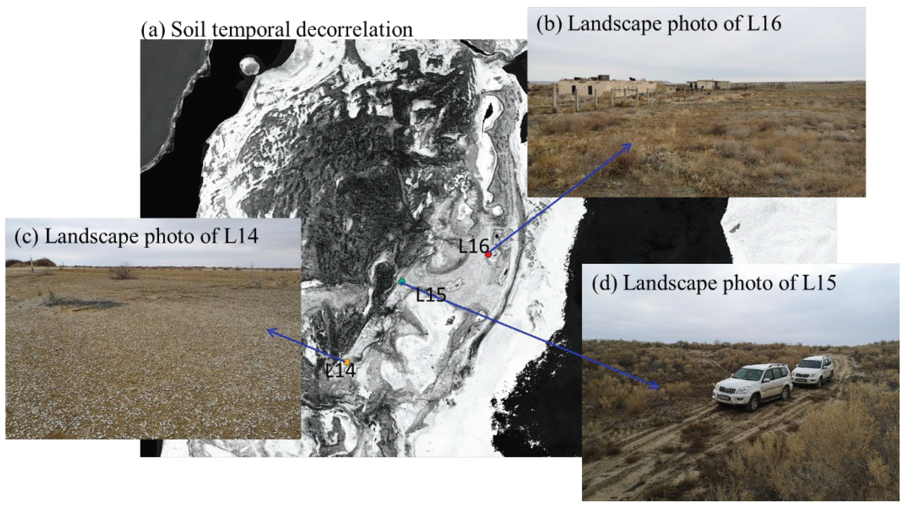
Table 2.
Sample statistics of the WEI at the dry bottom of the Aral Sea.
| Interval number | SITD interval | SITD interval | Percent (%) |
|---|---|---|---|
| 1 | .0000 | 0.1736 | |
| 2 | 3.7238 | ||
| 3 | 27.2261 | ||
| 4 | 15.4784 | ||
| 5 | 15.3211 | ||
| 6 | 35.5420 | ||
| 7 | 2.2560 | ||
| 8 | 0.2790 | ||
| total | 100 | ||
Disclaimer/Publisher’s Note: The statements, opinions and data contained in all publications are solely those of the individual author(s) and contributor(s) and not of MDPI and/or the editor(s). MDPI and/or the editor(s) disclaim responsibility for any injury to people or property resulting from any ideas, methods, instructions or products referred to in the content. |
© 2024 by the authors. Licensee MDPI, Basel, Switzerland. This article is an open access article distributed under the terms and conditions of the Creative Commons Attribution (CC BY) license (http://creativecommons.org/licenses/by/4.0/).
Copyright: This open access article is published under a Creative Commons CC BY 4.0 license, which permit the free download, distribution, and reuse, provided that the author and preprint are cited in any reuse.


