Submitted:
05 March 2024
Posted:
06 March 2024
Read the latest preprint version here
Abstract
Partial Information Decompositions (PIDs) aim to categorize how a set of source variables provide information about a target variable redundantly, uniquely, or synergetically. The original proposal for such an analysis used a lattice-based approach and gained significant attention. However, finding a suitable underlying decomposition measure is still an open research question, even at an arbitrary number of discrete random variables. This work proposes a solution to this case with a non-negative PID that satisfies an inclusion-exclusion relation for any f-information measure. The decomposition is constructed from a pointwise perspective of the target variable to take advantage of the equivalence between the Blackwell and zonogon order in this setting. We prove that the decomposition satisfies the axioms of the original decomposition framework and guarantees non-negative partial information results. We highlight that our decomposition behaves differently depending on the used information measure, which can be utilized for different applications. We additionally show how our proposal can be used to obtain a non-negative decomposition of Rényi-information at a transformed inclusion-exclusion relation, and for tracing partial information flows through Markov chains.
Keywords:
partial information decomposition
; redundancy
; synergy
; information flow analysis
; f-information
; rényi-information
1. Introduction
From computer science to neuroscience, we can find the following problem: We would like to know information about a random variable T, called the target, that we cannot observe directly. However, we can obtain information about the target indirectly from another set of variables . We can use information measures to quantify how much information any set of variables provides about the target. When doing so, we can identify the concept of redundancy: For example, if we have two identical variables , then we can use one variable to predict the other and thus anything that this other variable can predict. Similarly, we can identify the concept of synergy: For example, if we have two independent variables and a target that corresponds to their XOR operation , then both variables provide no advantage on their own for predicting the state of T, yet their combination fully determines it. Williams and Beer [1] suggested that it is possible to characterize information as visualized by the Venn diagram for two variables in Figure 1a. This decomposition attributes the total information about the target to being redundant, synergetic, or unique to a particular variable. As indicated in Figure 1a by , we can quantify three of the areas using information measures. However, this is insufficient to determine the four partial areas that represent the individual contributions. This causes the necessity to extend an information measure to either quantify the amount of redundancy or synergy between a set of variables.
Williams and Beer [1] first proposed a framework for Partial Information Decompositions (PIDs) and found favor by the community [2]. However, the proposed measure of redundancy was criticized for not distinguishing ”the same information and the same amount of information“ [3,4,5,6]. The proposal of Williams and Beer [1] focused specifically on mutual information. This work additionally studies the decomposition of any f-information or Rényi-information at discrete random variables. They have significance, among others, in parameter estimations, high-dimensional statistics, hypothesis testing, channel coding, data compression and privacy analyses [7,8].
1.1. Related Work
Most of the literature focuses on the decomposition of mutual information. Here, many alternative measures have been proposed but cannot suitably replace the original measure of Williams and Beer [1]: They are either limited to two observable variables [5,9,10], provide negative partial contributions [11,12,13], or provide results in which the partial contributions do not sum to the total amount [14]. Griffith et al. [3] studied the decomposition of zero-error information and obtained negative partial contributions. Kolchinsky [14] proposed a decomposition framework that is applicable beyond Shannon information theory, however, where the partial contributions do not sum to the total amount.
In this work, we propose a decomposition measure for replacing the one presented by William and Beer’s [14] while maintaining its desired properties. To achieve this, we combine several concepts from the literature: We use the Blackwell order, a preorder of information channels, for the decomposition and for deriving its operational interpretation, similar to Bertschinger et al. [9] and Kolchinsky [14]. We use its special case for binary input channels, the zonogon order studied by Bertschinger and Rauh [15], to achieve non-negativity at an arbitrary number of variables and provide it with a practical meaning. To utilize this special case for a general decomposition, we use the concept of a target pointwise decomposition as demonstrated by Williams and Beer [1] and related to Lizier et al. [16], Finn and Lizier [11], and Ince [12]. Finally, we apply the concepts from measuring on lattices, discussed by Knuth [17], to transform a non-negative decomposition with inclusion-exclusion relation from one information measure to another while maintaining the decomposition properties.
1.2. Contributions
In a recent work [18], we presented a decomposition of mutual information on the redundancy lattice (Figure 1b). This work aims to simplify, generalize and extend these ideas to make the following contributions to the area of Partial Information Decompositions:
- We propose a representation of distinct uncertainty and distinct information, which is used to demonstrate the unexpected behavior of the measure by Williams and Beer [1] (Section 2.2 and Section 3).
- We propose a decomposition for any f-information on both the redundancy lattice (Figure 1b) and synergy lattice (Figure 1c) that satisfies an inclusion-exclusion relation and provides a meaningful operational interpretation (Section 3.2).
- We prove that the proposed decomposition satisfies the original axioms of Williams and Beer [1] and guarantees non-negative partial information (Theorem 3).
- We propose to transform the non-negative decomposition of one information measure into another. This transformation maintains the non-negativity and its inclusion-exclusion relation under a re-definition of information addition (Section 3.3).
- We demonstrate the transformation of an f-information decomposition into a decomposition for Rényi- and Bhattacharyya-information (Section 3.3).
- We demonstrate that the proposed decomposition obtains different properties from different information measures and analyze the behavior of total variation in more detail (Section 4).
- We demonstrate the analysis of partial information flows through Markov chains (Figure 1) for each information measure on both the redundancy and synergy lattice (Section 4.2).
2. Background
This section aims to provide the required background information and introduce the used notation. Section 2.1 discusses the Blackwell order and its special case at binary targets, the zonogon order, which will be used for operational interpretations and the representation of f-information for its decomposition. Section 2.2 discusses the PID framework of Williams and Beer [1] and the relation between a decomposition based on the redundancy lattice and one based on the synergy lattice. We also demonstrate the unintuitive behavior of the original decomposition measure which will be resolved by our proposal in Section 3. Section 2.3 provides the considered definitions of f-information, Rényi-information, and Bhattacharyya information for the later demonstration of transforming decomposition results between measures.
Notation 1
(Random variables and their distribution). We use the notation T (upper case) to represent a random variable, ranging over the event space (calligraphic) containing events (lower case), and use the notation (P with subscript) to indicate its probability distribution. The same convention applies to other variables, such as a random variable S with events and distribution . We indicate the outer product of two probability distributions as , which assigns the product of their marginals to each event of the Cartesian product . Unless stated otherwise, we use the notation T, S and V to represent random variables throughout this work.
2.1. Blackwell and Zonogon Order
Definition 1
(Channel). A channel from to represents a garbling of the input variable T that results in variable S. Within this work, we represent an information channel μ as (row) stochastic matrix, where each element is non-negative, and all rows sum to one.
For the context of this work, we consider a variable S to be the observation of the output from an information channel from the target variable T, such that the corresponding channel can be obtained from their conditional probability distribution, as shown in Equation 1 where and .
Notation 2
(Binary input channels). Throughout this work, we reserve the symbol κ for binary input channels, meaning κ signals a stochastic matrix of dimension . We use the notation to indicate a column of this matrix.
Definition 2
(More informative [15,19]). An information channel is more informative than another channel if - for any decision problem involving a set of actions and a reward function that depends on the chosen action and state of the variable T - an agent with access to can always achieve an expected reward at least as high as another agent with access to .
Definition 3
Blackwell 19 showed that a channel is more informative if and only if it is Blackwell superior. Bertschinger and Rauh [15] showed that the Blackwell order does not form a lattice for channels if since the ordering does not provide unique meet and join elements. However, binary target variables are a special case where the Blackwell order is equivalent to the zonogon order (discussed next) and does form a lattice [15].
Definition 4
The zonogon is a centrally symmetric convex polygon, and the set of vectors span its perimeter. Figure 2 shows the example of a binary input channel and its corresponding zonogon.
Definition 5
(Zonogon sum). The addition of two zonogons corresponds to their Minkowski sum as shown in Equation 4.
Definition 6
(Zonogon order [15]). A zonogon is zonogon superior to another if and only if .
Bertschinger and Rauh [15] showed that for binary input channels, the zonogon order is equivalent to the Blackwell order and forms a lattice (Equation 5). In the remaining work, we will only discuss binary input channels, such that the orderings of Definition 2, 3 and 6 are equivalent and can be thought of as zonogons with subset relation.
For obtaining an interpretation of what a channel zonogon represents, we can consider a binary decision problem by aiming to predict the state of a binary target variable T using the output of channel . Any decision strategy for obtaining a binary prediction can be fully characterized by its resulting pair of True-Positive Rate (TPR) and False-Positive Rate (FPR), as shown in Equation 6
Therefore, a channel zonogon provides the set of all achievable (TPR,FPR)-pairs for a given channel [18,20]. This can also be seen from Equation 3, where the unit cube represents all possible first columns of the decision strategy . The first column of fully determines the second since each row has to sum to one. As a result, provides the (TPR,FPR)-pair for the decision strategy and the definition of Equation 3 all achievable (TPR,FPR)-pairs for predicting the state of a binary target variable. Since this will be helpful for operational interpretations, we label the axis of zonogon plots accordingly, as shown in Figure 2, and refer to regions within this plot as reachable decision regions:
Definition 7
(Reachable decision region). A reachable decision region for a binary decision problem is a set of achievable (TPR,FPR) performance pairs and can be visualized in a TPR/FPR-plot such as Figure 2.
Notation 3
(Channel lattice). We use the notation for the meet element of binary input channels under the Blackwell order and for their join element. We use the notation for the top element of binary input channels under the Blackwell order and for the bottom element.
For binary input channels, the meet element of the Blackwell order corresponds to the zonogon intersection and the join element of the Blackwell order corresponds to the convex hull of their union . Equation 7 describes this for an arbitrary number of channels.
2.2. Partial Information Decomposition
The commonly used framework for PIDs was introduced by Williams and Beer [1]. A PID is computed with respect to a particular random variable that we would like to know information about, called the target, and tries to identify from which variables that we have access to, called visible variables, we obtain this information. Therefore, this section considers sets of variables that represent their joint distribution.
Notation 4.
Throughout this work, we use the notation T for the target variable and for the set of visible variables. We use the notation for the power set of , and for its power set without the empty set.
Definition 8
(Sources, Atoms [1]).
- A source is a non-empty set of visible variables.
- An atoms is a set of sources constructed by Equation 8.
The used filter for obtaining the set of atoms (Equation 8) removes sets that would be equivalent to other elements. This is required for obtaining a lattice from the following two ordering relations:
Definition 9
The redundancy lattice for three visible variables is visualized in Figure 3a. On this lattice, we can think of an atom as representing the information that can be obtained from all of its sources about the target T (their redundancy or informational intersection). For example, the atom represents on the redundancy lattice the information that is contained in both and about T. Since both sources in provide the information of , their redundancy contains at least this information, and the atom is considered its predecessor. Therefore, the ordering indicates an informational subset relation for the redundancy of atoms, and the information that is represented by an atom increases as we move up. The up-set of an atom on the redundancy lattice indicates the information that is lost when losing all of its sources. Considering the example from above, if we lose access to and , then we lose access to all atoms in the up-set of .
Definition 10
(Synergy-/Loss-lattice [21]). The synergy lattice is obtained by applying the ordering relation of Equation 10 to all atoms .
The synergy lattice for three visible variables is visualized in Figure 3b. On this lattice, we can think of an atom as representing the information that is contained in neither of its sources (information outside their union). For example, the atom represents on the synergy lattice the information that is obtained from neither nor about T. The ordering again indicates their expected subset relation: the information that is obtained from neither nor is fully contained in the information that cannot be obtained from and thus is a predecessor of .
With an intuition for both ordering relations in mind, we can see how the filter in the construction of atoms (Equation 8) removes sets that would be equivalent to another atom: the set is removed from the power set of sources since it would be equivalent to the atom under the ordering of the redundancy lattice and equivalent to the atom under the ordering of the synergy lattice.
Notation 5
(Redundancy/Synergy lattices). We use the notation for the join and meet operators on the redundancy lattice, and for the join and meet operators on the synergy lattice. We use the notation for the top and for the bottom atom on the redundancy lattice, and and for the top and bottom atom on the synergy lattice. For an atom α, we use the notation for its down-set, for its strict down-set, and for its cover set. These definitions will only appear in the Möbius inverse of a function that is directly associated with either the synergy or redundancy lattice such that there is no ambiguity about which ordering relation has to be considered.
The redundant, unique, or synergetic information (partial contributions) can be calculated based on either lattice. They are obtained by quantifying each atom of the redundancy or synergy lattice with a cumulative measure that increases as we move up in the lattice. The partial contributions are then obtained in a second step from a Möbius inverse.
Definition 11
([Cumulative] redundancy measure [1]). A redundancy measure is a function that assigns a real value to each atom of the redundancy lattice. It is interpreted as a cumulative information measure that quantifies the redundancy between all sources of an atom about the target T.
Definition 12
([Cumulative] loss measure [21]). A loss measure is a function that assigns a real value to each atom of the synergy lattice. It is interpreted as a cumulative measure that quantifies the information about T that is provided by neither of the sources of an atom .
To ensure that a redundancy measure actually captures the desired concept of redundancy, Williams and Beer [1] defined three axioms that a measure should satisfy. For the synergy lattice, we consider the equivalent axioms discussed by Chicharro and Panzeri [21]:
Axiom 1
Axiom 2
Axiom 3
The first axiom states that an atom’s redundancy and information loss should not depend on the order of its sources. The second axiom states that adding sources to an atom can only decrease the redundancy of all sources (redundancy lattice) and decrease the information from neither source (synergy lattice). The third axiom binds the measures to be consistent with mutual information and ensures that the bottom element of both lattices is quantified to zero.
Once a lattice with corresponding cumulative measure (/) is defined, we can use the Möbius inverse to compute the partial contribution of each atom. This partial information can be visualized as partial area in a Venn diagram (see Figure 1a) and corresponds to the desired redundant, unique, and synergetic contributions. However, the same atom represents different partial contributions on each lattice: As visualized for the case of two visible variables in Figure 1, the unique information of variable is represented by on the redundancy lattice and by on the synergy lattice.
Definition 13
Remark 2.
Using the Möbius inverse for defining partial information enforces an inclusion-exclusion relation in that all partial information contributions have to sum to the corresponding cumulative measure. Kolchinsky [14] argues that an inclusion-exclusion relation should not be expected to hold for PIDs and proposes an alternative decomposition framework. In this case, the sum of partial contributions (unique/redundant/synergetic information) is no longer expected to sum to the total amount .
Property 1
The non-negativity property is important if we assume an inclusion-exclusion relation since it states that the unique, redundant, or synergetic information cannot be negative. If an atom provides a negative partial contribution in the framework of Williams and Beer [1], then this may indicate that we over-counted some information in its down-set.
Remark 3.
Several additional axioms and properties have been suggested since the original proposal of Williams and Beer [1], such as target monotonicity and target chain rule [4]. However, this work will only consider the axioms and properties of Williams and Beer [1]. To the best of our knowledge, no other measure since the original proposal (discussed below) has been able to satisfy these properties for an arbitrary number of visible variables while ensuring an inclusion-exclusion relation for their partial contributions.
It is possible to convert between both representations due to a lattice duality:
Definition 14
(Lattice duality and dual decompositions [21]). Let be a redundancy lattice with associated measure and let be a synergy lattice with measure , then the two decompositions are said to be dual if and only if the down-set on one lattice corresponds to the up-set in the other as shown in Equation 13.
Williams and Beer [1] proposed , as shown in Equation 14, to be used as measure of redundancy and demonstrated that it satisfies the three required axioms and local positivity. They define redundancy (Equation 14b) as the expected value of the minimum specific information (Equation 14a).
Remark 4.
Throughout this work, we use the term ’target pointwise information’ or simply ’pointwise information’ to refer to ’specific information’. This shall avoid confusion when naming their corresponding binary input channels in Section 3.
However, the measure could be criticized for not providing a notion of distinct information due to its use of a pointwise minimum (for each ) over the sources. This leads to the question of distinguishing ”the same information and the same amount of information“ [3,4,5,6]. We can use the definition through a pointwise minimum (Equation 14) to construct examples of unexpected behavior: consider for example a uniform binary target variable T and two visible variables as output of the channels visualized in Figure 4. The channels are constructed to be equivalent for both target states and provide access to distinct decision regions while ensuring a constant pointwise information .
Even though our ability to predict the target variable significantly depends on which of the two indicated channel outputs we observe (blue or green in Figure 4), the measure concludes full redundancy between them . We think this behavior is undesired and, as discussed in the literature, caused by an underlying lack of distinguishing the same information. To resolve this issue, we will present a representation of f-information in Section 3.1, which allows the use of all (TPR,FPR)-pairs for each state of the target variable to represent a distinct notion of uncertainty.
2.3. Information Measures
This section discusses two generalizations of mutual information at discrete random variables based on f-divergences and Rényi divergences [22,23]. While mutual information has interpretational significance in channel coding and data compression, other f-divergences have their significance in parameter estimations, high-dimensional statistics, and hypothesis testing [7, p. 88], while Rényi-divergences can be found among others in privacy analysis [8]. Finally, we introduce Bhattacharyya information for demonstrating that it is possible to chain decomposition transformations in Section 3.3. All definitions in this section only consider the case of discrete random variables (which is what we need for the context of this work).
Definition 15
- f is convex,
- ,
- is finite for all .
By convention we understand that and . For any such function f and two discrete probability distributions P and Q over the event space , the f-divergence for discrete random variables is defined as shown in Equation 15.
Notation 6.
Throughout this work, we reserve the name f for functions that satisfy the required properties for an f-divergence of Definition 15.
An f-divergence quantifies a notion of dissimilarity between two probability distributions P and Q. Key properties of f-divergences are their non-negativity, their invariance under bijective transformations, and them satisfying a data-processing inequality [7, p. 89]. A list of commonly used f-divergences is shown in Table 1. Notably, the continuation for of both the Hellinger- and -divergence result in the KL-divergence [24].
The generator function of an f-divergence is not unique since for a real constant [7]. As a result, the considered -divergence is a linear scaling of the Hellinger divergence () as shown in Equation 16.
Definition 16
Definition 17
(f-entropy). A notion of f-entropy for a discrete random variable is obtained from the self-information of a variable .
Notation 7.
Using the KL-divergence results in the definition of mutual information and Shannon entropy. Therefore, we use the notation for mutual information (KL-information) and (KL-entropy ) for the Shannon entropy.
The remaining part of this section will define Rényi- and Bhattacharyya-information to highlight that they can be represented as an invertible transformation of Hellinger-information. This will be used in Section 3.3 to transform the decomposition of Hellinger-information to a decomposition of Rényi- and Bhattacharyya-information.
Remark 5.
We could similarly choose to represent Renyi divergence as a transformation of the α-divergence. A liner scaling of the considered f-divergence will however not affect our later results (see Section 3.3).
Definition 18
Notably, the continuation of Rényi divergence for also equals the KL-divergence [7, p. 116]. Renyi divergence can be expressed as an invertible transformation of the Hellinger divergence (, see Equation 18) [24].
Definition 19
Finally, we consider the Bhattacharyya distance (Definition 20), which is equivalent to a linear scaling from a special case of Rényi divergence (Equation 20) [24]. It is applied, among others, in signal processing [25] and coding theory [26]. The corresponding information measure (Equation 21) is like its distance the scaling of a special case of Rényi-information.
Definition 20
Definition 21
(Bhattacharyya-information). Bhattacharyya-information is defined equivalent to f-information as shown in Equation 21.
3. Decomposition Methodology
To construct a partial information decomposition in the framework of Williams and Beer [1], we only have to define a cumulative redundancy measure () or cumulative loss measure (). However, doing this requires a meaningful definition of when information is the same. Therefore, Section 3.1 presents an interpretation of f-information that enables a representation of distinct information. Specifically, we demonstrate that f-information quantifies the expected perimeter for the channel zonogons of each state . This allows for the interpretation that each distinct (TPR,FPR)-pair for predicting a state of the target variable provides a distinct notion of uncertainty. Information corresponds accordingly to reachable decision regions, which are quantified by their perimeter. This interpretation of f-information is used in Section 3.2 to construct a partial information decomposition under the zonogon order for each state individually. These individual decompositions are then combined into the final result. Therefore, we decompose specific information based on the Blackwell order rather than using its minimum, like Williams and Beer [1]. We use the resulting decomposition of any f-information in Section 3.3 to transform a Hellinger-information decomposition into a Rényi-information decomposition while maintaining its non-negativity and an inclusion-exclusion relation. In Section 3.2 and Section 3.3, we first demonstrate the decomposition on the synergy lattice and then its corresponding dual decomposition on the redundancy lattice. To achieve the desired axioms and properties, we combine different aspects of the existing literature:
- In a similar manner to how Finn and Lizier [11] used probability mass exclusion to differentiate distinct information, we use the achievable decision regions for each state of a target variable to differentiate distinct information.
- We propose applying the concepts about lattice re-graduations discussed by Knuth [17] to PIDs to transform the decomposition of one information measure to another while maintaining its consistency.
We extend Axiom 3 of Williams and Beer [1] as shown below, to allow binding any information measure to the decomposition.
Axiom 3* (Self-redundancy).
For a single source, redundancy and information loss correspond to information measure as shown below:
3.1. Representing f-Information
We begin with an interpretation of f-information, for which we define a pointwise variable that represents one state of the target variable (Equation 23a) and construct its pointwise information channel (Definition 22). Then, we define a function based on the generator function of an f-divergence. This function acts like a pseudo-distance for measuring half the length of the zonogon perimeters for each pointwise information channel (see Figure 2). These zonogon perimeter lengths are pointwise f-information.
Definition 22
([Target] pointwise binary input channel). We define a target pointwise binary input channel from one state of the target variable to an information source with event space as shown in Equation 23b.
Definition 23
([Target] pointwise f-information).
- We define a function as shown in Equation 24a to quantify a vector, where .
- We define a target pointwise f-information function , as shown in Equation 24b, to quantify half the zonogon perimeter for the corresponding pointwise channel .
Theorem 1
(Properties of ). For a constant : (1) the function is convex in , (2) scales linearly in , (3) satisfies a triangle inequality in , (4) quantifies any vector of slope one to zero, and (5) quantifies the zero vector to zero.
Proof.
- The convexity of in is shown separately in Lemma A1 of Appendix A.
- That scales linearly in can directly be seen from Equation 24a.
- The triangle inequality of in is shown separately in Corollary A1 of Appendix A.
- A vector of slope one is quantified to zero , since is a requirement on the generator function of an f-divergence (Definition 15).
- The zero vector is quantified to zero by the convention of generator functions for an f-divergence (Definition 15).
□
The properties of the function are useful since we can interpret it as a pseudo-distance when quantifying the perimeter length of a channel zonogon . The function provides the following properties to the pointwise information measure .
Theorem 2
(Properties of ). The pointwise information measure (1) maintains the ordering relation of the Blackwell order for binary input channels and (2) is non-negative.
Proof.
- That the function maintains the ordering relation of the Blackwell order on binary input channels is shown separately in Lemma A2 of Appendix A (Equation 25a).
- The bottom element consists of a single vector of slope one, which is quantified to zero by Theorem 1 (Equation 25b). The combination with Equation 25a ensures the non-negativity.
□
An f-information corresponds to the expected value of the target pointwise f-information function defined above (Equation 26). As a result, we can interpret f-information as quantifying (half) the expected zonogon perimeter length for the pointwise channels , where the function acts as a pseudo-distance.
3.2. Decomposing f-Information
With the representation of Section 3.1 in mind, we can define a non-negative partial information decomposition for a set of visible variables about a target variable T for any f-information. The decomposition is performed from a pointwise perspective, which means that we decompose the pointwise measure on the synergy lattice for each . The pointwise synergy lattices are then combined using a weighted sum to obtain the decomposition of .
We map each atom of the synergy lattice to the join of pointwise channels for its contained sources.
Definition 24
(From atoms to channels). We define the channel corresponding to an atom as shown in Eqation 27.
Lemma 1.
For any set of sources and target variable T with state , the function maintains the ordering of the synergy lattice under the Blackwell order as shown in Equation 28.
Lemma 1 is shown separately in Section B.1 of Appendix B. The mapping from Definition 24 provides a lattice that can be quantified using pointwise f-information to construct a cumulative loss measure for its decomposition using the Möbius inverse.
Definition 25
([Target] pointwise cumulative and partial loss measures). We define the target pointwise cumulative and partial loss functions as shown in Equation 29a and 29b.
The combined cumulative and partial measures are the expected value of their corresponding pointwise measures. This corresponds to combining the pointwise decomposition lattices by a weighted sum.
Definition 26
Theorem 3.
The presented definitions for the pointwise and expected loss measures ( and ) provide a non-negative PID on the synergy lattice with inclusion-exclusion relation that satisfies the Axioms 1, 2 and 3* for any f-information measure.
Proof.
- Axiom 1: The measure (Equation 29a) is invariant to permuting the order of sources in , since the join operator of the zonogon order () is. Therefore, also satisfies Axiom 1.
- Axiom 2: The monotonicity of both and on the synergy lattice is shown separately as Corollary A2 in Appendix B.
- Non-negativity: The non-negativity of and is shown separately as Lemma A7 in Appendix B.
□
Consider the pointwise and combined redundancy measures ( and ) as shown in Equation 32, which are defined through an additional inclusion-exclusion relation on the sources of an atom (pointwise using Equation 32a and 32b or combined using Equation 32c). The partial contributions ( and ) are obtained from the Möbius inverse. This defines the corresponding dual decomposition on the redundancy lattice.
Definition 27
(Dual decomposition on the redundancy lattice). We define the pointwise and cumulative redundancy measure as shown in Equation 32.
Corollary 1.
The dual decomposition as defined by Equation 32 provides a non-negative PID which satisfies an inclusion-exclusion relation and the axioms of Williams and Beer [1] on the redundancy lattice.
Proof.
The Axioms 1 and 3* are transformed from Theorem 3 by Equation 32c. The non-negativity is obtained from Theorem 3 since the partial contributions are identical between dual decompositions. The non-negativity ensures monotonicity (Axiom 2) since the cumulative measure is the sum of (non-negative) partial contributions in its down-set due to the Möbius inverse. □
Remark 6.
As discussed before [18], it is possible to further split the redundant component in the decomposition for extracting the pointwise meet under the Blackwell order (zonogon intersection). The second component of redundancy as defined above contains decision regions that are part of the convex hull but not the individual channel zonogons (discussed as shared information in [18]).
From a pointwise perspective, there always exists a dependency between the sources for which the synergy of this state becomes zero. This dependence corresponds, by definition, to the join of their channels. This is helpful for the operational interpretation in the following paragraph since, individually, each pointwise synergy becomes fully volatile to the dependence between the sources.
Operational interpretation: The decomposition obtains the operational interpretation that if a variable provides pointwise unique information, then there exists a unique decision region for some that this variable provides access to. Moreover, if a set of variables provides synergetic information, then a decision region for some may become inaccessible if the dependence between the variables changes. Due to the equivalence of the zonogon and Blackwell order for binary input variables, these interpretations can also be transferred to a set of actions and a pointwise reward function , which only depends on one state of the target variable (see Section 2.1): If a variable provides unique information, then it provides an advantage for some set of actions and pointwise reward function, while synergy indicates that the advantage for some pointwise reward function is based on the dependence between variables.
The implication of the interpretation does not hold in the other direction, which we will also highlight in the example of in Section 4.1. Finally, the definition of the Blackwell order through the chaining of channels (Equation 2) highlights its suitability for tracing the flows of information in Markov chains (see Section 4.2).
3.3. Decomposing Rényi-Information
Since Rényi-information is an invertible transformation of Hellinger-information and -information, we argue that their decompositions should be consistent. We propose to view the decomposition of Rényi-information as a transformation from an f-information and demonstrate the approach by transferring the Hellinger-information decomposition to a Rényi-information decomposition. Then, we demonstrate that the result is invariant to a linear scaling of the considered f-information, such that the transformation from -information provides identical results. The obtained Rényi-information decomposition is non-negative and satisfies the three axioms proposed by Williams and Beer [1] (see below). However, its inclusion-exclusion relation is based on a transformed addition operator. For transforming the decomposition, we consider Rényi-information to be a re-graduation of Hellinger-information, as shown in Equation 33.
To maintain consistency when transforming the measure, we also have to transform its operators [17, p. 6 ff.]:
Definition 28
(Addition of Rényi-information). We define the addition of Rényi-information with its corresponding inverse function by Equation 34.
To transform a decomposition of the synergy lattice, we define the cumulative loss measures as shown in Equation 35 and use the transformed operators when computing the Möbius inverse (Equation 36a) to maintain consistency in the results (Equation 36b).
Definition 29.
The cumulative and partial Rényi-information loss measures are defined as transformations of the cumulative and partial Hellinger-information loss measures, as shown in Equation 35 and 36.
Remark 7.
We show in Lemma A8 of Appendix C that re-scaling the original f-information does not affect the resulting decomposition or transformed operators. Therefore, transforming a Hellinger-information decomposition or a α-information decomposition to a Rényi-information decomposition provides identical results.
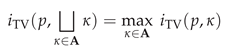
The operational interpretation presented in Section 3.2 is similarly applicable to partial Rényi-information ( , Equation 36b), since the function satisfies and .
Theorem 4.
The presented definitions for the cumulative loss measure provide a non-negative PID on the synergy lattice with inclusion-exclusion relation under the transformed addition (Definition 28) that satisfies the Axioms 1, 2 and 3* for any Rényi-information measure.
Proof.
- Axiom 1: is invariant to permuting the order of sources, since satisfies Axiom 1 (see Section 3.2).
- Axiom 2: satisfies monotonicity, since satisfies Axiom 2 (see Section 3.2) and the transformation function is monotonically increasing for .
- Axiom 3*: Since satisfies Axiom 3* (see Section 3.2, Equation 33 and 35), satisfies the self-redundancy axiom by definition, however, at a transformed operator: .
- Non-negativity: The decomposition of is non negative, since is non-negative (see Section 3.2), the Möbius inverse is computed with transformed operators (Equation 36b) and the function satisfies .
□
Remark 8.
To obtain an equivalent decomposition of Rényi-information on the redundancy lattice, we can correspondingly transform the dual decomposition from the redundancy lattice of Hellinger-Information as shown in Equation 37. The resulting decomposition will satisfy the non-negativity, axioms of Williams and Beer [1] and an inclusion-exclusion relation under the transformed operators (Definition 28) for the same reasons described above from Corollary 1.
Remark 9.
When taking the limit of Rényi-information for , we obtain mutual information (). Since mutual information is also an f-information, we expect its operators in the Möbius inverse to be addition. This is indeed the case (Equation 38), and the measures will be consistent.
Finally, the decomposition of Bhattacharyya-information can be obtained by re-scaling the decomposition of Rényi-information at , which causes another transform of the addition operator for the inclusion-exclusion relation.
4. Evaluation
A comparison of the proposed decomposition with other methods of the literature can be found in [18] for mutual information. Therefore, this section first compares different f-information measures at typical decomposition examples and discusses the special case of total variation (TV)-information to explain its distinct behavior. Since we can see larger differences between measures in more complex scenarios, we compare the measures by analyzing the information flows in a Markov chain. We provide the used implementation for both dual decompositions of f-information and the examples used in this work at [28].
4.1. Partial Information Decomposition
4.1.1. Comparison of Different f-Information Measures
We use the examples discussed by Finn and Lizier [11] to compare different f-information decompositions and add a generic example from [18]. All used probability distributions and their abbreviations can be found in Appendix D. We normalize the decomposition results to the f-Entropy of the target variable for the visualization in Figure 5.
Since all results are based on the same framework, they behave similarly at examples that analyze a specific aspect of the decomposition function (XOR, Unq, PwUnq, RdnErr, Tbc, AND). However, it can be observed that the decomposition of total variation (TV) appears to differ from others: (1) In all examples, total variation attributes more information to being redundant than other measures. (2) In the generic example, total variation is the only measure that does not attribute any information to being unique to variable one or synergetic. We discuss the case of total variation in Section 4.1.2 to explain its distinct behavior.
We visualize the zonogons for the generic example in Figure A2, which shall highlight that the implication of the operational interpretation does not hold in the other direction: the existence of partial information implies an advantage for the expected reward towards some state of the target variable, but an advantage for the expected reward towards some state of the target variable does not imply partial information in the example of total variation.
4.1.2. The Special Case of Total Variation
The behavior of total variation appears different compared to other f-information measures (Figure 5). This is due to total variation measuring the perimeter of a zonogon such that the result corresponds to a linear scaling of the maximal (Euclidean) height that the zonogon reaches above the diagonal as visualized in Figure 6:
Lemma 2.
- a)
- b)
- For a non-empty set of pointwise channels , pointwise total variation quantifies the join element to the maximum of its individual channels (Equation 39b).
- c)
- The loss measure quantifies the meet for a set of sources on the synergy lattice to their minimum (Equation 39c).
Proof.
The proof of the first two statements (Equation 39b and 39b) is provided separately in Appendix E, which imply the third (Equation 39c) by Definition 25. □
Quantifying the meet element on the synergy lattice to the minimum has the following consequences for total variation: (1) It attributes a minimum amount of synergy, and therefore more information to redundancy than other measures. (2) For each state of the target, at most one variable can provide unique information. In the case of , the pointwise channels are symmetric (see Equation 6), such that the same variable provides the maximal zonogon height both times. This is the case in the generic example of Figure 5, and the reason why at most one variable can provide unique information in this setting. However, beyond binary targets (), both variables may provide unique information at the same time since different sources can provide the maximal zonogon height for different target states (see later example in Figure 7).
Remark 10.
Using the pointwise minimum on the synergy lattice results in a similar structure to the proposed measure of Williams and Beer [1]. However, TV-information is based on a different pointwise measure , which displays the same behavior (Equation 39b), unlike pointwise KL-information.
4.2. Information Flow Analysis
The differences between f-information measures in Section 4.1 appear more visible in complex scenarios. Therefore, this section compares different measures in the information flow analysis of a Markov chain.
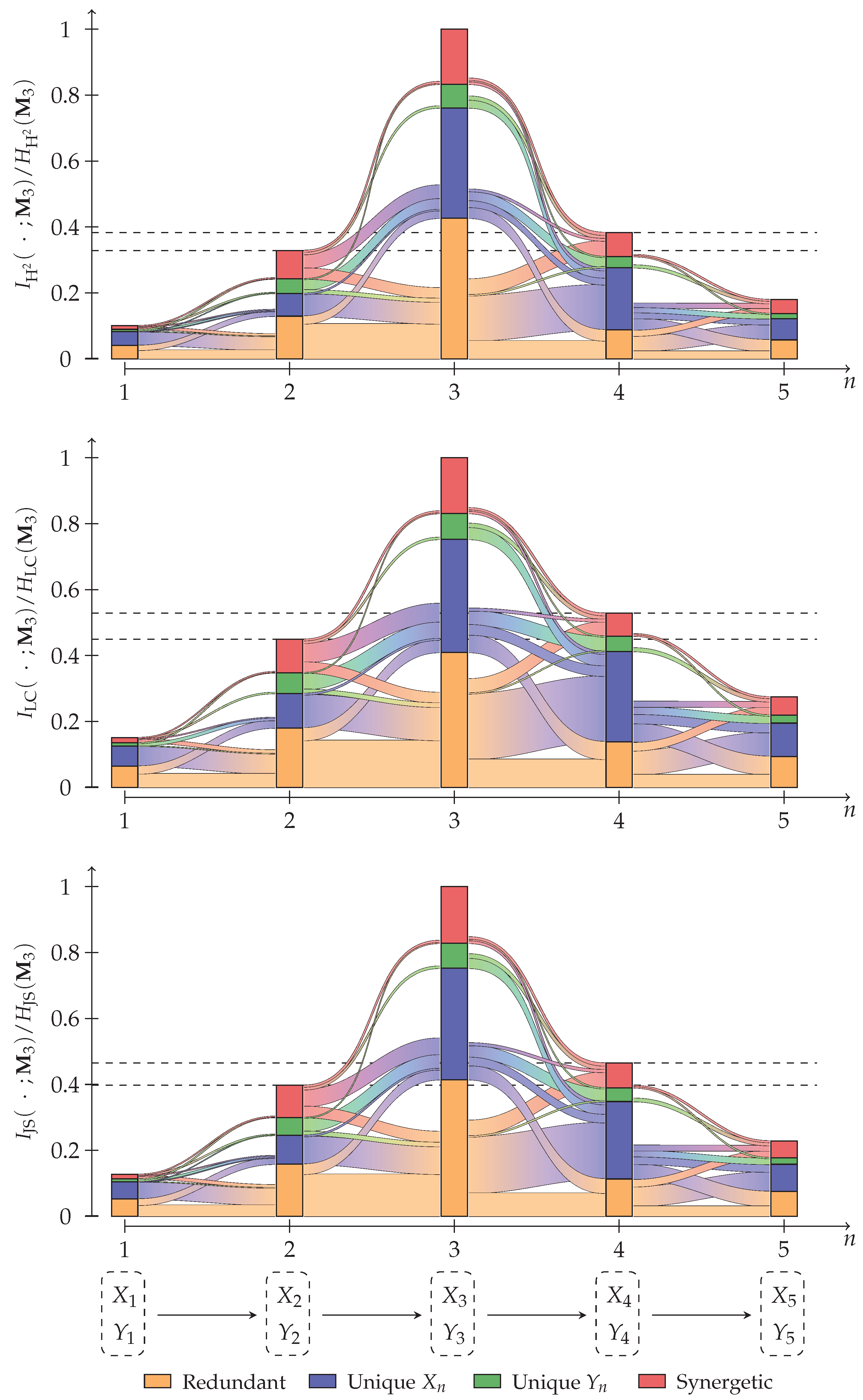
Consider a Markov chain , where is the joint distribution of two variables. Assume that we are interested in state three and thus define as the target variable. Using the approach described in Section 3, we can compute an information decomposition for each state of the Markov chain with respect to the target. Now, we are additionally interested in how the partial information decomposition from stage propagates into the next , as visualized in Figure 7.
Definition 30
(Partial information flow). The partial information flow of an atom into the atom quantifies the redundancy between the partial contributions of their respective decomposition lattices.
Notation 8.
We use the notation with to refer to either the loss measure or redundancy measure . The same applies to the functions and of Equation 40.
Let and , then we compute information flows equivalently on the redundancy or synergy lattice as shown in Equation 40. When using a redundancy measure , then the strict down-set of refers to the strict down-set on its redundancy lattice and when using a loss measure , then the strict down-set refers to the strict down-set on its synergy lattice . We obtain the intersection of cumulative measures by quantifying their meet, which is on both lattice equivalent to their union of sources (, Equation 40a). To obtain how much of the partial contribution of can be found in the cumulative measure of (), we remove the contributions of its down-set ( on lattice for , see Equation 40b). To finally obtain the flow from the partial contribution of to the partial contribution of (), we similarly remove the contributions of the down-set of ( on lattice for , see Equation 40c). The approach can be extended for tracing information flows over multiple steps, however, we will only trace one step in this example.
Remark 11.
The resulting partial information flows are equivalent (dual) between the redundancy and loss measure except for the bottom element since their functionality differs: The flow from or to the bottom element on the redundancy lattice is always zero. In contrast, the flow from or to the bottom element on the synergy lattice quantifies the information gained or lost in the step.
Remark 12.
The information flow analysis of Rényi- and Bhattacharyya-information can be obtained as a transformation of the information flow from Hellinger-information. Alternatively, the information flow can be computed directly using Equation 40 under the corresponding definition of addition and subtraction for the used information measure.
Figure 7.
Analysis of the Markov chain information flow (Equation A27). Visualized results for the information measures: KL, TV, and . The remaining results (-, LC-, and JS-information) can be found in Figure A3.
Figure 7.
Analysis of the Markov chain information flow (Equation A27). Visualized results for the information measures: KL, TV, and . The remaining results (-, LC-, and JS-information) can be found in Figure A3.
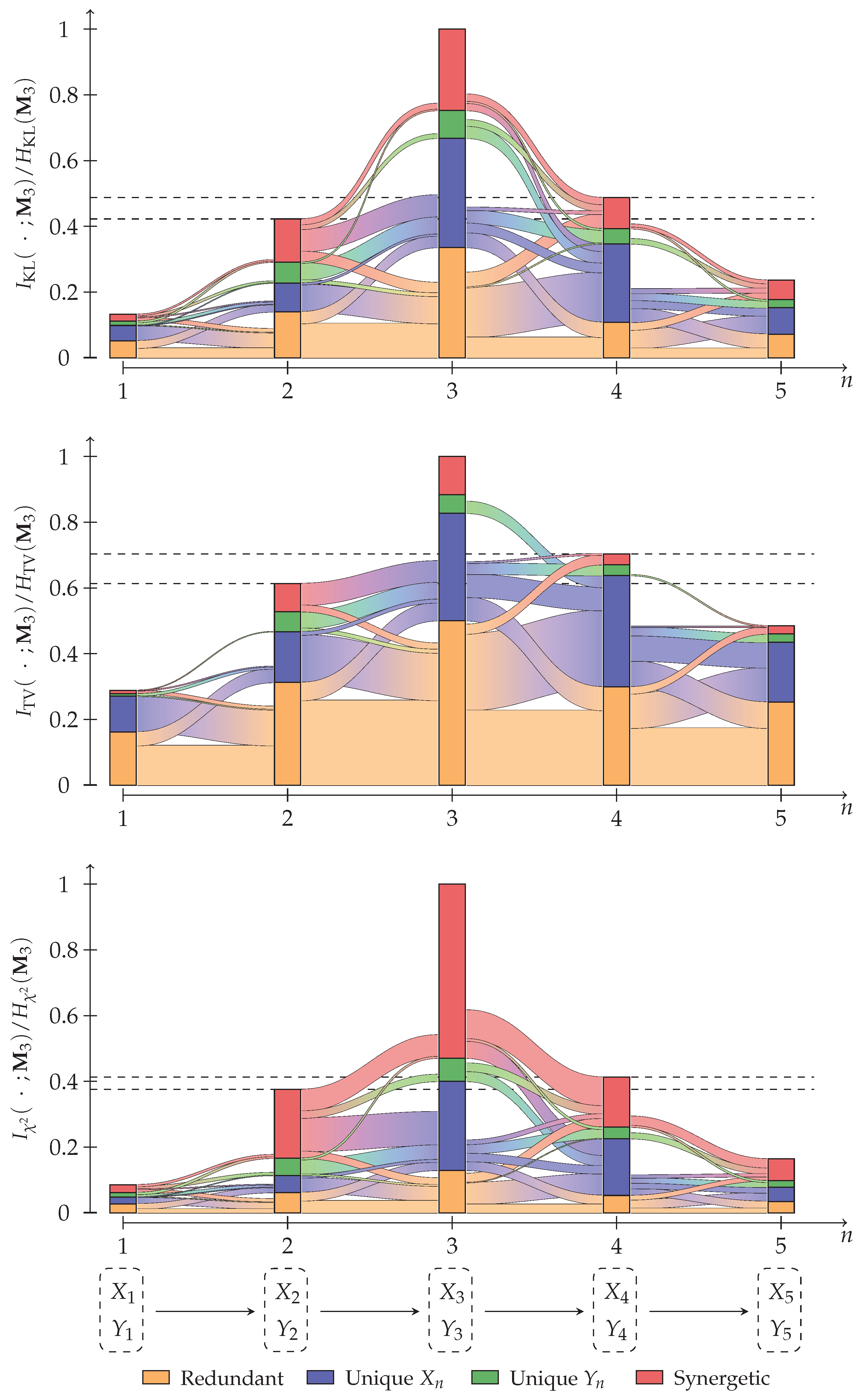
We randomly generate an initial distribution and each row of a transition matrix under the constraint that at least one value shall be above 0.8 to avoid an information decay that is too rapid through the chain. The specific parameters of the example are shown in Appendix F. The used event spaces are and such that . We construct a Markov chain of five steps with the target and trace each partial information for one step using Equation 40. We visualized the results for KL-, TV-, and -information in Figure 7, and the results for -, LC- and JS-information in Figure A3 of Appendix F.
All results display the expected behavior that the information that provides about increases for and decreases for . The information flow results of KL-, -, LC-, and JS-information are conceptually similar. Their main differences appear in the rate at which the information decays and, therefore, how much of the total information we can trace. In contrast, the results of TV- and -information display different behavior, as shown in Figure 7: TV-information indicates significantly more redundancy, and -information displays significantly more synergy than the other measures. Additionally, the decomposition of TV-information contains fever information flows. For example, it is the only analysis that does not show any information flow from into the unique contribution of or from into the synergy of . This demonstrates that the same decomposition method can obtain different behaviors from different f-divergences.
5. Discussion
We perform the decomposition on a pointwise lattice using the zonogon join since it is possible to represent f-information as quantification of the zonogon perimeter on pointwise channels. Correspondingly, if we identified an information measure that was based on quantifying the zonogons of the pointwise channels by their area, then we would need to decompose it on a pointwise lattice using the zonogon meet to achieve non-negativity.
In the literature, PIDs have been defined based on different ordering relations [14]. This diversity is desirable since each approach provides a different operational interpretation of redundancy and synergy. For this reason, we wonder if obtaining a non-negative decomposition with inclusion-exclusion relation for other ordering relations was possible when transferring them to a pointwise perspective or from mutual information to other information measures.
We think studying the relations between different information measures for the same decomposition method may provide further insights into their properties, as demonstrated by the example of total variation in Section 4.2. Similarly, allowing the re-definition of addition for different information measures, as demonstrated in the example of Rényi-information in Section 3.3, opens new possibilities for satisfying the inclusion-exclusion relation and providing consistent decomposition results between related information measures.
Finally, there is currently no universally accepted definition of conditional Rényi information. Assuming that should capture the information that provides about T when already knowing the information from , then one could propose that this quantity should correspond to the according partial information contributions (unique/synergetic) and thus the definition of Equation 41.
6. Conclusions
In this work, we demonstrated a non-negative PID in the framework of Williams and Beer [1] for any f-information with practical operational interpretation. We demonstrated that the decomposition of f-information can be used to obtain a non-negative decomposition of Rényi-information, for which we re-defined the addition to demonstrate that its results satisfy an inclusion-exclusion relation. Finally, we demonstrated how the proposed decomposition method can be used for tracing the flow of information through Markov chains and how the decomposition obtains different properties depending on the chosen information measure.
Author Contributions
Conceptualization, Writing - original draft: T.M.; Analysis of non-negativity: T.M. and E.A.; Writing - review & editing: E.A. and C.R.; Supervision: C.R.
Funding
This research was funded by Swedish Civil Contingencies Agency (MSB) through the project RIOT grant number MSB 2018-12526.
Conflicts of Interest
The authors declare no conflict of interest. The funders had no role in the design of the study; in the collection, analyses, or interpretation of data; in the writing of the manuscript; or in the decision to publish the results.
Appendix A. Quantifying Zonogon Perimeters
Lemma A1.
If the function f is convex, then the function as defined in Equation 24a is convex in its second argument () for a constant and .
Proof.
We use the following definitions for abbreviating the notation. Let and :
The case of is handled by the convention that . Therefore, we can assume that and use with to apply the definition of convexity on the function f:
□
Corollary A1.
For a constant and , the function as defined in Equation 24a satisfies a triangle inequality on its second argument: .
Proof.
□
Lemma A2.
For a constant , the function maintains the ordering relation from the Blackwell order on binary input channels: .
Proof.
Let be represented by a matrix and by a matrix. By the definition of the Blackwell order (, Equation 2), there exists a stochastic matrix such that . We use the notation to refer to the column of matrix and indicate the element at row and column of by . Since is a valid (row) stochastic matrix of dimension , its rows sum to one .
□
Lemma A3.
Consider two non-empty sets of binary input channels with equal cardinality () and a constant . If the Minkowski sum for the zonogons of channels in is a subset of the Minkowski sum for the zonogons of channels in , then the sum of pointwise information for the channels in is less than the sum of pointwise information for the channels in as shown in Equation A1.
Proof.
Let . We use the notation with to indicate the channel within the set .
□
Appendix B. The Non-Negativity of Partial f-Information
The proof of non-negativity can be divided into three parts. First, we show that the loss measure maintains the ordering relation of the synergy lattice and how the quantification of a meet element can be computed. Second, we demonstrate the construction of a bijective mapping between all subsets of even and odd cardinality that maintains a required subset relation for any selection function. Finally, we combine these two results to demonstrate that an inclusion-exclusion relation using the convex hull of zonogons is greater than their intersection and obtain the non-negativity of the decomposition by transitivity.
Appendix B.1. Properties of the Loss Measure on the Synergy Lattice
We require some of the following properties to hold for any set of sources . Therefore, we define an equivalence relation from the ordering of the synergy lattice (≅) as shown in Equation A2.
Notation A1
(Equivalence under synergy-ordering). We use the notation for the equivalence of two sets of sources on the synergy lattice.
Lemma A4.
Any set of sources is equivalent (≅) to some atom of the synergy lattice .
The union for two sets of sources is equivalent to the meet of their corresponding atoms on the synergy lattice. Let and :
Proof.
The used filter in the definition of an atom (, Equation 8) only removes sets of cardinality and for any removed set of sources, we can construct an equivalent set which contains one less source by removing the subset as shown in Equation A3a. Therefore, all sets of sources are equivalent to some atom within the lattice (Equation A3b).
The union of two sets of sources is inferior to each individual set and :
All sets of sources that are inferior of both and ( and ) are also inferior to their union.
Therefore, the union of and is equivalent to the meet of their corresponding atoms on the synergy lattice. □
Proof of Lemma 1 from Section 3.2:
For any set of sources and target variable T with state , the function (Equation 27) maintains the ordering from the synergy lattice under the Blackwell order.
Proof.
We consider two cases for :
- If , then the implication holds for any since the bottom element is inferior (⊑) to any other channel.
- If , then is also a non-empty set since .
Since the implication holds for both cases, the ordering is maintained. □
Corollary A2.
Proof.
Corollary A3.
The cumulative pointwise loss of the meet from two atoms is equivalent to the cumulative pointwise loss of their union for any target variable T with state :
.
Proof.
The result follows from Lemma A4 and Corollary A2. □
Appendix B.2. Mapping Subsets of Even and Odd Cardinality
Let represent the power-set of a non-empty set and separate the subsets of even () and odd () cardinality as shown below. Additionally, let represent all subsets with cardinality less or equal to one and all subsets of cardinality equal to one:
The number of subsets with even cardinality is equal to the number of subsets with odd cardinality as shown in Equation A6.
Consider a function , which takes an even subset and returns a subset of cardinality according to Equation A7.
Lemma A5.
For any function , there exists a function which satisfies the following two properties:
- a)
- For any subset with even cardinality, the function returns a subset of function :
- b)
- The function which satisfies Equation A8 has an inverse on its first argument .
Figure A1.
Intuition for the definition of Equation A11. We can divide the set into and . The definition of function mirrors if (blue) and otherwise breaks its mapping (orange).
Figure A1.
Intuition for the definition of Equation A11. We can divide the set into and . The definition of function mirrors if (blue) and otherwise breaks its mapping (orange).
Proof.
We construct a function G for an arbitrary and demonstrate that it satisfies both properties (Equation A8 and A9) by induction on the cardinality of . We indicate the cardinality of with as subscript , , and :
-
At the base case , the sets of subsets are and . We define the function for any to satisfy both required properties:
-
For the induction step, we show the definition of a function that satisfies both required properties. For sets , the subsets of even and odd cardinality can be expanded as shown in Equation A10.We define for and at any as shown in Equation A11 using the function and its inverse from the induction hypothesis. The function is defined for any subset in as it can be seen from Equation A10.Figure A1 provides an intuition for the definition of : the outcome of determines, if the function maintains or breaks the mapping of .The function F as defined in Equation A11 satisfies both requirements (Equation A8 and A9) for any :
- a)
-
To demonstrate that the function satisfies the subset relation of Equation A8, we analyze the four cases for the return value of as defined in Equation A11 individually:
- holds, since the function always returns a subset of its input (Equation A7).
- holds by the induction hypothesis.
- if then : Since the input to function is not the empty set, the function returns a singleton subset of its input (Equation A7). If the element in the singleton subset is unequal to q, then it is a subset of .
- if then holds trivially.
- b)
-
To demonstrate that the function has an inverse (Equation A9), we show that the function is a bijection from to . Since the function is defined for all elements in and both sets have the same cardinality (, Equation A6), it is sufficient to show that the function is distinct for all inputs.The return value of has four cases, two of which return a set containing q (case 1 and 4 in Equation A11), while the two others do not (case 2 and 3 in Equation A11). Therefore, we have to show that both of these cases cannot coincide for any input:
- -
- Case 2 and 3 in Equation A11: If the return value of both cases was equal, then and therefore . This leads to a contradiction, since the condition of case 3 ensures , while the condition of case 2 ensures . Hence, the return values of case 2 and 3 are distinct.
- -
- Case 1 and 4 in Equation A11: If the return value of both cases was equal, then and therefore . This leads to a contradiction, since the condition of case 4 ensures , while the condition of case 1 ensures . Hence, the return values of case 1 and 4 are distinct.
Since the function is a bijection, there exists an inverse .
□
Appendix B.3. The non-negativity of the decomposition
Lemma A6.
Consider a Non-Empty Set of of Binary Input Channel and . Quantifying an inclusion-exclusion principle on the pointwise information of their Blackwell join is larger than the pointwise information of their Blackwell meet as shown in Equation A12.
Proof.
Consider a function , where such that the function returns a singleton subset for a set of odd cardinality. Equation A13 can be obtained from the constraints on (Equation A7) and Lemma A5.
Equation A14a holds since we can replace with , meaning there exists a for creating a (Minkowski) sum over the same set of channel zonogons on both sides of the quality. Equation A14b holds since Lemma A5 ensured that the existing function G is a bijection. Equation A14c holds since the intersection is a subset of each individual zonogon.
Equation A14c is parameterized by and subsets are closed under set union. Therefore, we can combine all choices for and using the set-theoretic union as shown below. For the notation, let and we indicate subsets of with even cardinality as , where . We use the last index for the empty set . The subsets of with odd cardinality are correspondingly noted as . For clarity, we note binary input channels from an even subset as and binary input channels from an odd subset as .
□
Lemma A7.
The decomposition of f-information is non-negative on the pointwise and combined synergy lattice for any target variable T with state :
Proof.
We show the non-negativity of pointwise partial information () in two cases . We write to represent the cover set of on the synergy lattice and use as abbreviation:
-
Let , then its cover set is non-empty (). Additionally, we know that no atom in the cover set is the empty set (), since the empty atom is the top element ().Since it will be required later, note that the inclusion-exclusion principle of a constant is the constant itself as shown in Equation A16 since without the empty set there exists one more subset of odd cardinality than with even cardinality (see Equation A6).We can re-write the Möbious inverse as shown in Equation A17.Consider the non-empty set of channels , then we obtain Equation A18b from Lemma A6.We can construct an upper bound on based on the cover set as shown in Equation A19.By transitivity of Equation A18b and A19d, we obtain Equation A20.By Equation A17 and A20, we obtain the non-negativity of pointwise partial information as shown in Equation A21.
From Equation A15 and A21, we obtain that pointwise partial information is non-negative for all atoms of the lattice:
If all pointwise partial components are non-negative, then their expected value will also be non-negative (see Equation 31):
□
Appendix C. Scaling f-information does not affect its transformation
Lemma A8.
The Linear Scaling of an f-Information Does Not Affect the Transformation Result and Operator: Consider Scaling an f-Information Measure with , then their decomposition transformation to another measure will be equivalent.
Proof.
Based on the definitions of Section 3.2, the loss measures scale linear with the scaling of their f-divergence. Therefore, we obtain two cumulative loss measures, where and are a linear scaling of each other (Equation A24a). They can be transformed into another measure , as shown in Equation A24b.
Equation A24b already demonstrates that their transformation results will be equivalent and that and . Therefore, their operators will also be equivalent as shown below:

Appendix D. Decomposition Example Distributions
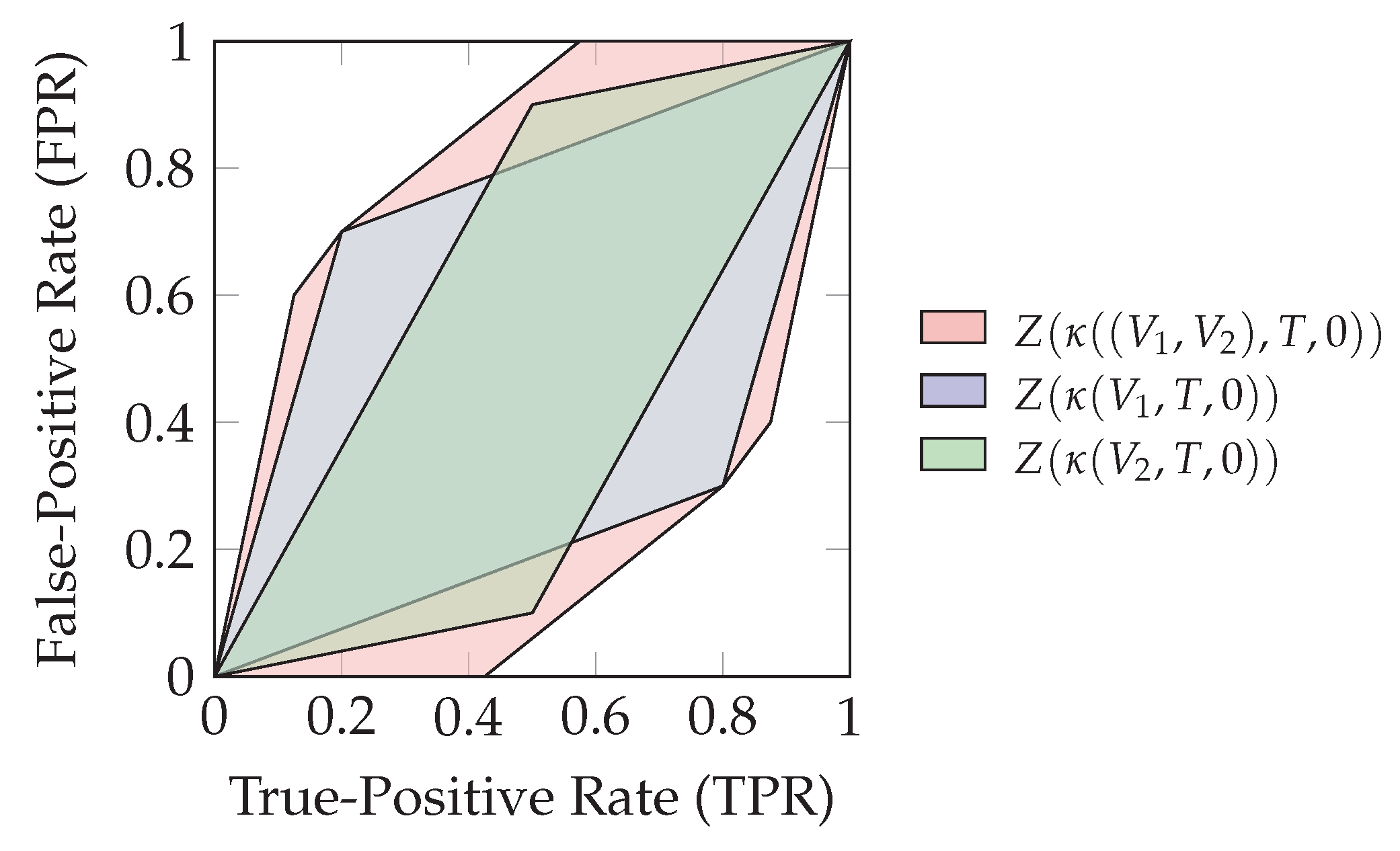
The probability distributions used in Figure 5 can be found in Table A1. For providing an intuition of the decomposition result for IU,TV at the generic example, we visualized its corresponding zonogons in Figure A2. It can be seen that the maximal zonogon height is obtained from V1 (blue) which equals the maximal zonogon height of their joint distribution (V1,V2) (red). Therefore, IU,TV does not attribute partial information uniquely to V2 or their synergy by Lemma 2.

Table A1.
The used distributions from [11] and the generic example from [18]. The example names are abbreviations for: XOR-gate (XOR), Unique (Unq), Pointwise Unique (PwUnq), Redundant-Error (RdnErr), Two-Bit-copy (Tbc) and the AND-gate (AND) [11].
Table A1.
The used distributions from [11] and the generic example from [18]. The example names are abbreviations for: XOR-gate (XOR), Unique (Unq), Pointwise Unique (PwUnq), Redundant-Error (RdnErr), Two-Bit-copy (Tbc) and the AND-gate (AND) [11].
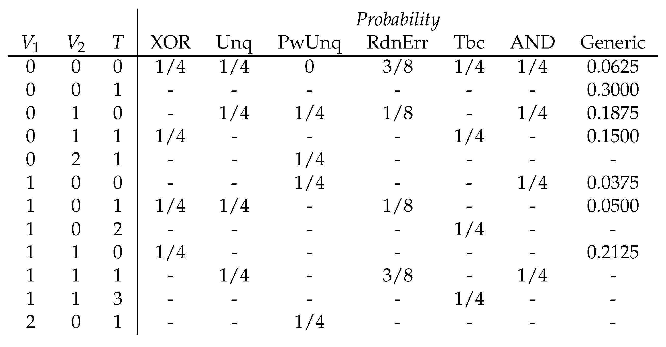 |
Figure A2.
Visualization of the zongons from the generic example of [18] at state t = 0. The target variable T has two states. Therefore, the zonogons of its second state are symmetric (second column of Equation 6) and have identical heights.
Figure A2.
Visualization of the zongons from the generic example of [18] at state t = 0. The target variable T has two states. Therefore, the zonogons of its second state are symmetric (second column of Equation 6) and have identical heights.
Appendix E. The Relation of Total Variation to the Zonogon Height
Proof of Lemma 2 a) from Section 4.1.2:
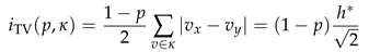
The pointwise total variation (iTV) is a linear scaling of the maximal (Euclidean) height h* that the corresponding zonogon Z(K) reaches above the diagonal as visualized in Figure 6 for any 0 ≤ p ≤ 1.
Proof.
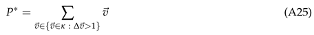
The point of maximal height P* that a zonogon Z(K) reaches above the diagonal is visualized in Figure 6 and can be obtained as shown in Equation A25, where  represents the slope of vector
represents the slope of vector
The maximal height (Euclidean distance) above the diagonal is calculated as shown in Equation A26, where 

The pointwise total variation iTV can be expressed as invertible transformation of the maximal euclidean zonogon height above the diagonal as shown in Equation E, where 
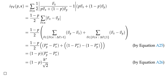
Proof of Lemma 2 b) from Section 4.1.2:
For a non-empty set of pointwise channel A and 0 ≤ p ≤ 1, pointwise total variation iTV quantifies the join element to the maximum of its individual channels:
Proof.
The join element  corresponds to the convex hull of all individual zonogons (see Equation 7). The maximal height that the convex hull reaches above the diagonal is equal to the maximum of the maximal height that each individual zonogon reaches. Since pointwise total variation
is a liner scaling of the (Euclidean) zonogon height above the diagonal (Lemma 2 a) shown above), the join element is valuated to the maximum of its individual channels. □
corresponds to the convex hull of all individual zonogons (see Equation 7). The maximal height that the convex hull reaches above the diagonal is equal to the maximum of the maximal height that each individual zonogon reaches. Since pointwise total variation
is a liner scaling of the (Euclidean) zonogon height above the diagonal (Lemma 2 a) shown above), the join element is valuated to the maximum of its individual channels. □Appendix F. Information Flow Example Parameters and Visualization
The parameters for the Markov chain used in Section 4.2 are shown in Equation A27, where Mn = (Xn,Yn), Xi = {0, 1, 2}, Yi = {0, 1}, PM1 is the initial distribution and PMn+1|Mn is the transition
matrix. The visualized results for the information flow of KL-, TV-, and X2-information can be found
in Figure 7, and the visualized results of H2-, LC-, and JS-information in Figure A3.
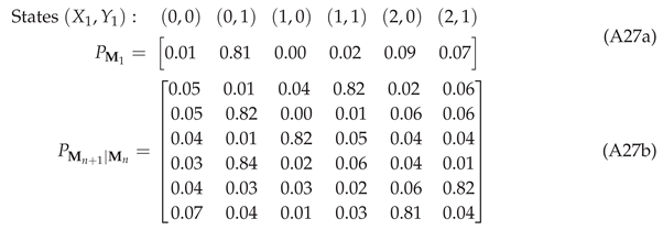
Figure A3.
Analysis of the Markov chain information flow (Equation A27). Visualized results for the information measures: H2, LC, and JS. The remaining results (KL, TV, and X2) can be found in Figure 7.
Figure A3.
Analysis of the Markov chain information flow (Equation A27). Visualized results for the information measures: H2, LC, and JS. The remaining results (KL, TV, and X2) can be found in Figure 7.
References
- Williams, P.L.; Beer, R.D. Nonnegative Decomposition of Multivariate Information. arXiv 2010, arXiv:1004.2515. [Google Scholar]
- Lizier, J.T.; Bertschinger, N.; Jost, J.; Wibral, M. Information Decomposition of Target Effects from Multi-Source Interactions: Perspectives on Previous, Current and Future Work. Entropy 2018, 20. [Google Scholar] [CrossRef]
- Griffith, V.; Chong, E.K.P.; James, R.G.; Ellison, C.J.; Crutchfield, J.P. Intersection Information Based on Common Randomness. Entropy 2014, 16, 1985–2000. [Google Scholar] [CrossRef]
- Bertschinger, N.; Rauh, J.; Olbrich, E.; Jost, J. Shared Information—New Insights and Problems in Decomposing Information in Complex Systems. In Proceedings of the Proceedings of the European Conference on Complex Systems 2012; 2013; pp. 251–269. [Google Scholar]
- Harder, M.; Salge, C.; Polani, D. Bivariate measure of redundant information. Phys. Rev. E 2013, 87, 012130. [Google Scholar] [CrossRef]
- Finn, C. A New Framework for Decomposing Multivariate Information. PhD thesis, University of Sydney, 2019.
- Polyanskiy, Y.; Wu, Y. Information theory: From coding to learning. Book draft 2022.
- Mironov, I. Renyi Differential Privacy. In Proceedings of the 2017 IEEE 30th Computer Security Foundations Symposium (CSF); 2017; pp. 263–275. [Google Scholar] [CrossRef]
- Bertschinger, N.; Rauh, J.; Olbrich, E.; Jost, J.; Ay, N. Quantifying Unique Information. Entropy 2014, 16, 2161–2183. [Google Scholar] [CrossRef]
- Griffith, V.; Koch, C. , Heidelberg, 2014; pp. 159–190. https://doi.org/10.1007/978-3-642-53734-9_6.Information. In Guided Self-Organization: Inception; Springer Berlin Heidelberg: Berlin, Heidelberg, 2014; pp. 159–190. [Google Scholar] [CrossRef]
- Finn, C.; Lizier, J.T. Pointwise Partial Information Decomposition Using the Specificity and Ambiguity Lattices. Entropy 2018, 20. [Google Scholar] [CrossRef]
- Ince, R.A.A. Measuring Multivariate Redundant Information with Pointwise Common Change in Surprisal. Entropy 2017, 19. [Google Scholar] [CrossRef]
- Rosas, F.E.; Mediano, P.A.M.; Rassouli, B.; Barrett, A.B. An operational information decomposition via synergistic disclosure. Journal of Physics A: Mathematical and Theoretical 2020, 53, 485001. [Google Scholar] [CrossRef]
- Kolchinsky, A. A Novel Approach to the Partial Information Decomposition. Entropy 2022, 24. [Google Scholar] [CrossRef]
- Bertschinger, N.; Rauh, J. The Blackwell relation defines no lattice. In Proceedings of the 2014 IEEE International Symposium on Information Theory; 2014; pp. 2479–2483. [Google Scholar] [CrossRef]
- Lizier, J.T.; Flecker, B.; Williams, P.L. Towards a synergy-based approach to measuring information modification. In Proceedings of the 2013 IEEE Symposium on Artificial Life (ALife); 2013; pp. 43–51. [Google Scholar] [CrossRef]
- Knuth, K.H. Lattices and Their Consistent Quantification. Annalen der Physik 2019, 531, 1700370. [Google Scholar] [CrossRef]
- Mages, T.; Rohner, C. Decomposing and Tracing Mutual Information by Quantifying Reachable Decision Regions. Entropy 2023, 25. [Google Scholar] [CrossRef]
- Blackwell, D. Equivalent comparisons of experiments. The annals of mathematical statistics, 1953; 265–272. [Google Scholar]
- Neyman, J.; Pearson, E.S. IX. On the problem of the most efficient tests of statistical hypotheses. Philosophical Transactions of the Royal Society of London. Series A, Containing Papers of a Mathematical or Physical Character 1933, 231, 289–337. [Google Scholar]
- Chicharro, D.; Panzeri, S. Synergy and Redundancy in Dual Decompositions of Mutual Information Gain and Information Loss. Entropy 2017, 19. [Google Scholar] [CrossRef]
- Csiszar, I. On information-type measure of difference of probability distributions and indirect observations. Studia Sci. Math. Hungar. 1967, 2, 299–318. [Google Scholar]
- Renyi, A. On measures of entropy and information. In Proceedings of the Proceedings of the Fourth Berkeley Symposium on Mathematical Statistics and Probability, Volume 1: Contributions to the Theory of Statistics.; 1961; Volume 4, pp. 547–562. [Google Scholar]
- Sason, I.; Verdu, S. f -Divergence Inequalities. IEEE Transactions on Information Theory 2016, 62, 5973–6006. [Google Scholar] [CrossRef]
- Kailath, T. The divergence and Bhattacharyya distance measures in signal selection. IEEE transactions on communication technology 1967, 15, 52–60. [Google Scholar] [CrossRef]
- Arikan, E. Channel Polarization: A Method for Constructing Capacity-Achieving Codes for Symmetric Binary-Input Memoryless Channels. IEEE Transactions on Information Theory 2009, 55, 3051–3073. [Google Scholar] [CrossRef]
- Bhattacharyya, A. On a measure of divergence between two statistical populations defined by their probability distribution. Bulletin of the Calcutta Mathematical Society 1943, 35, 99–110. [Google Scholar]
- Mages, T.; Anastasiadi, E.; Rohner, C. Implementation: PID Blackwell specific information. https://github.com/uucore/pid-blackwell-specific-information, 2024.
Figure 1.
Partial information decomposition representations at two variables . (a) Visualization of the desired intuition for multivariate information as Venn diagram. (b) Representation as redundancy lattice, where quantifies the information that is contained in all of its provided variables (inside their intersection). The ordering represents the expected subset relation of redundancy. (c) Representation as synergy lattice, where quantifies the information that is contained in neither of its provided variables (outside their union). (d) When having two partial information decompositions with respect to the same target variable, we can study how the partial information of one decomposition propagates into the next. We refer to this as information flow analysis of a Markov chain such as .
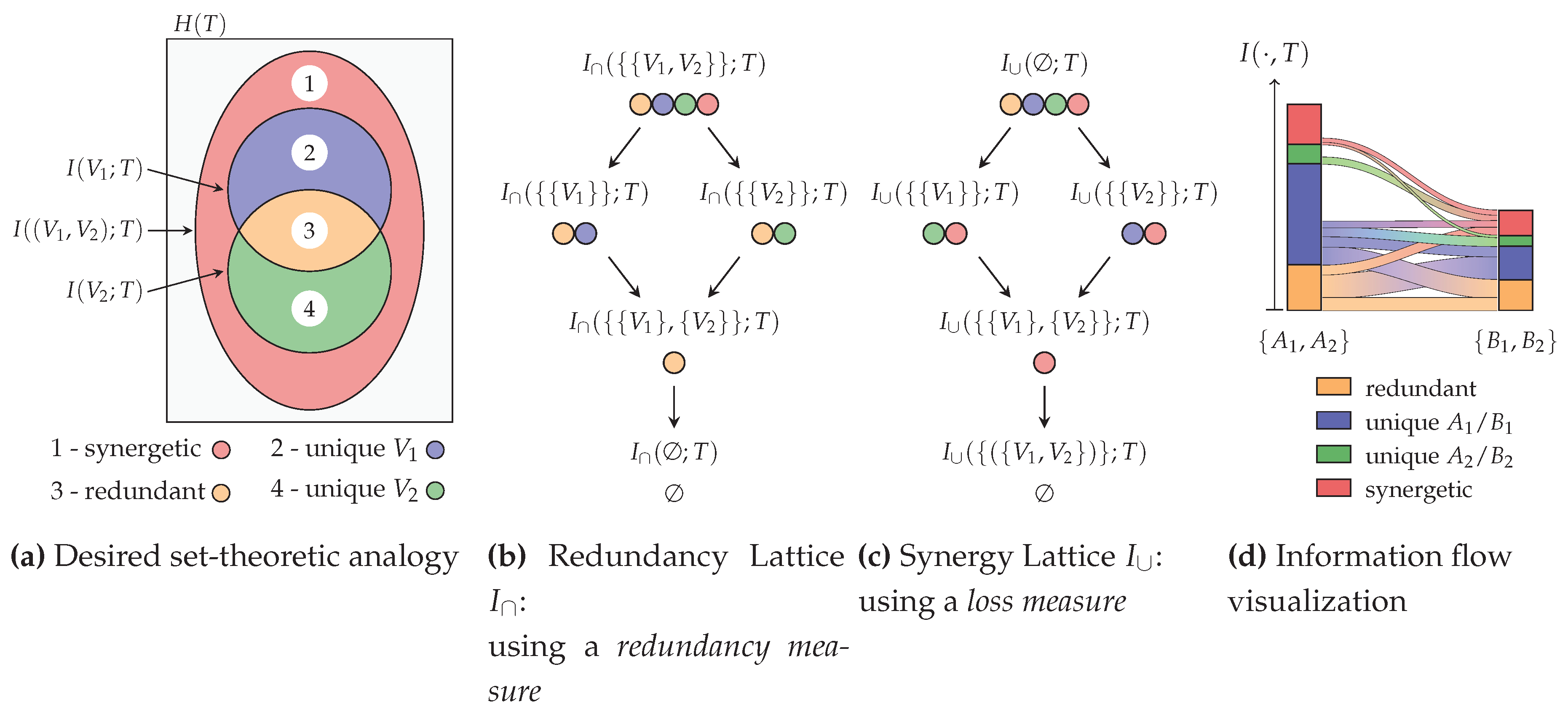
Figure 2.
An example zonogon (blue) for a binary input channel . The zonogon perimeter corresponds to the vectors sorted by increasing/decreasing slope for the lower/upper half. The zonogon also corresponds to the set of (TPR,FPR)-pairs that are achievable when predicting the binary target variable.
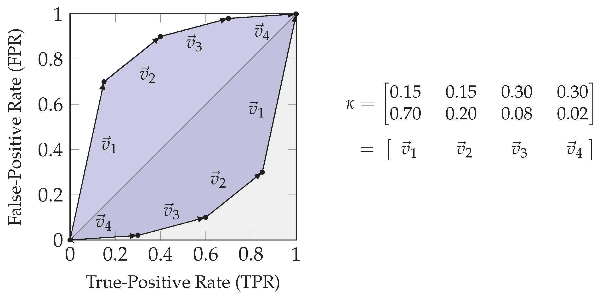
Figure 3.
For the visualization, we abbreviated the notation by indicating the contained visible variable as index of the source, for example, to represent their joint distribution: (a) A redundancy lattice based on the ordering ≼ of Equation 9. (b) A synergy lattice based on the ordering ⪯ of Equation 10 for the partial information decomposition at . On the redundancy lattice, the redundancy of all sources within an atom increases while moving up. On the synergy lattice, the information that is obtained from neither source of an atom increases while moving up.
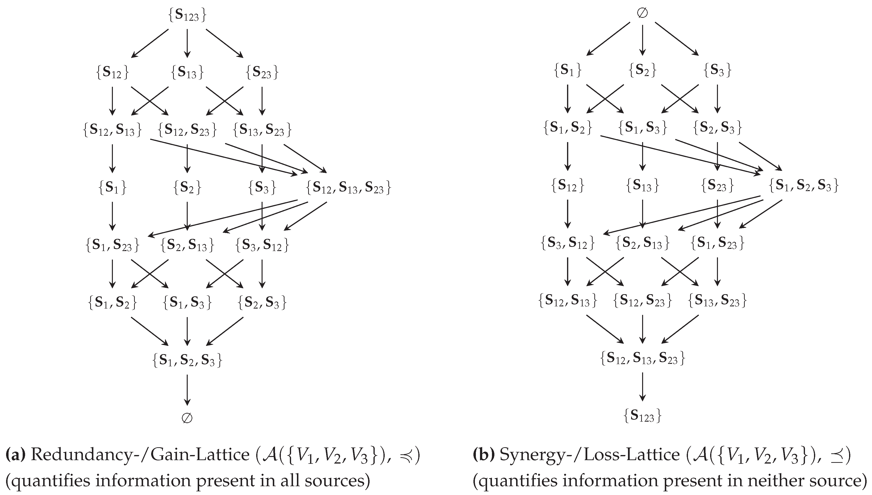
Figure 4.
Example of the unexpected behavior of : the dashed isoline indicates the pairs for which channel results in a pointwise information for a uniform binary target variable. Even though observing the output of both indicated example channels (blue/green) provides significantly different abilities for predicting the target variable state, the measure indicates full redundancy.
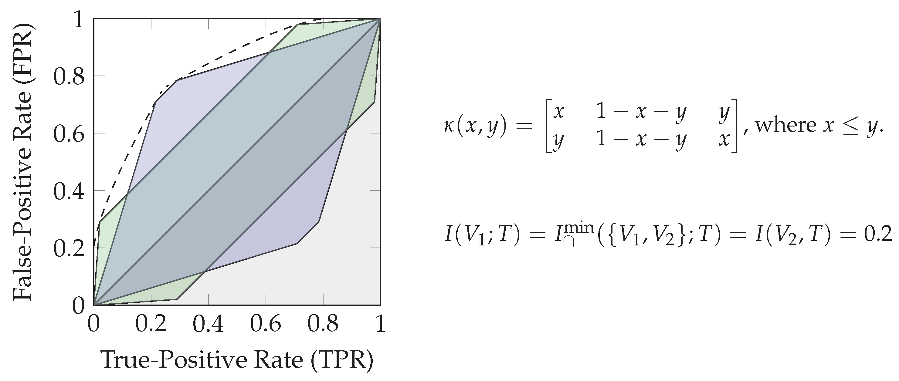
Figure 5.
Comparison of different f-information measures normalized to the f-Entropy of the target variable. All distributions are shown in Appendix D and correspond to the examples of [11,18]. The example name abbreviations are listed below Table A1. The measures behave mostly similarly since the decompositions follow an identical structure. However, it can be seen that total variation attributes more information to being redundant than other measures and appears to behave differently in the generic example since it does not attribute any partial information to the first variable or their synergy.
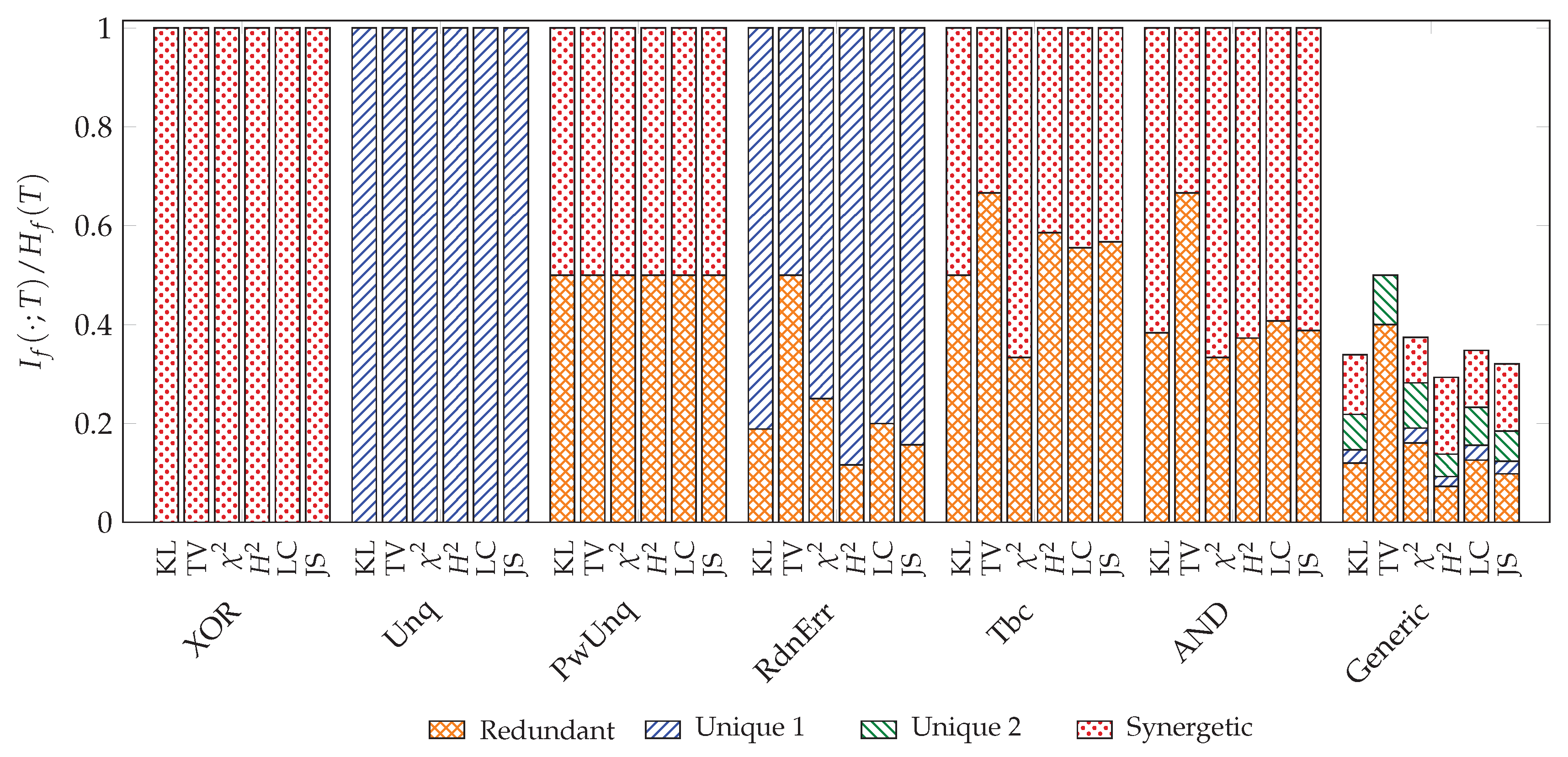
Figure 6.
Visualization of the maximal (Euclidean) height at point that a zonogon (blue) reaches above the diagonal.
Figure 6.
Visualization of the maximal (Euclidean) height at point that a zonogon (blue) reaches above the diagonal.
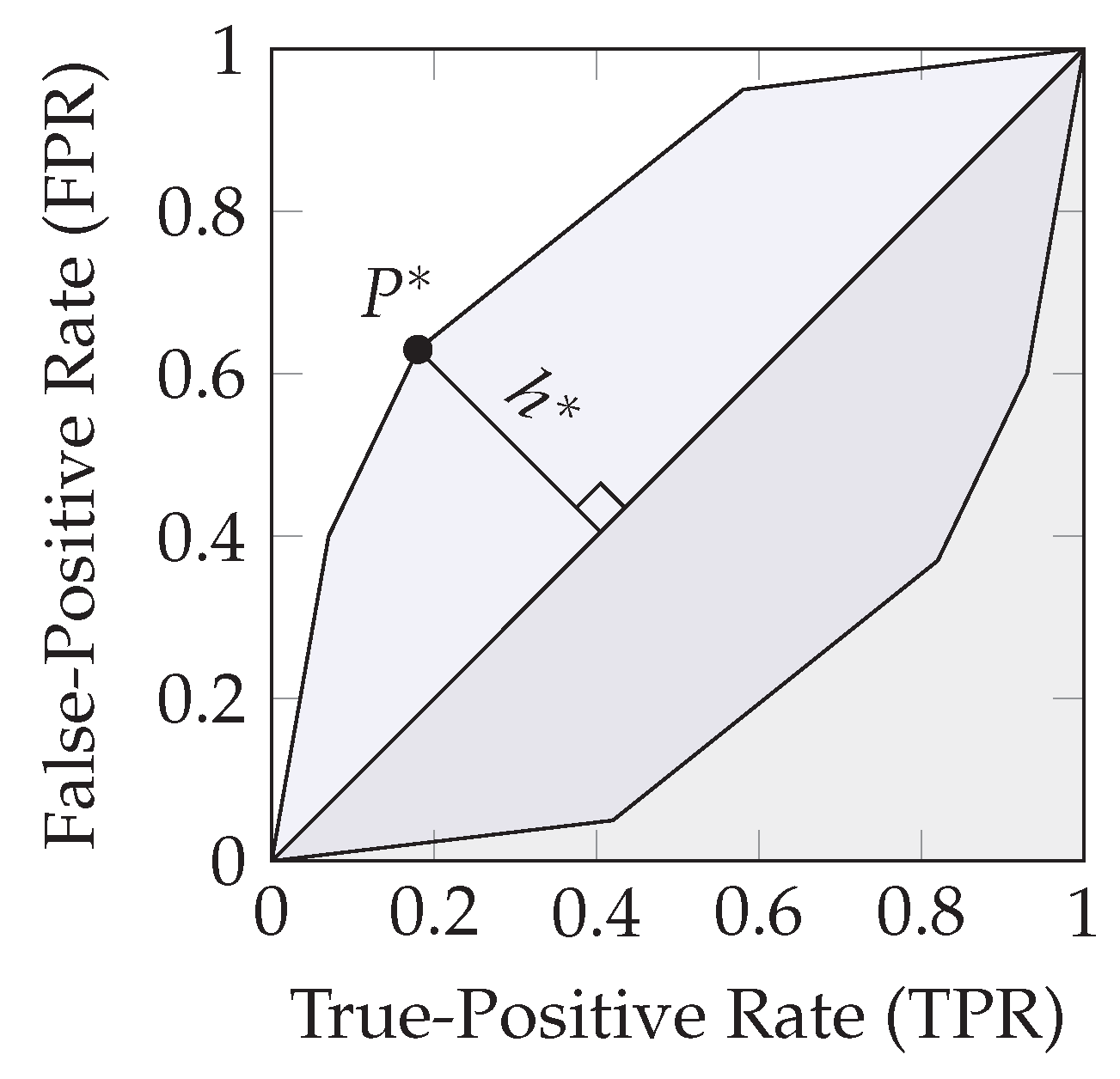
Table 1.
Commonly used functions for f-divergences.
| KL divergence | ||
| TV | ||
| -divergence | ||
| Squared Hellinger distance | ||
| Le Cam distance | ||
| Jensen-Shannon divergence | ||
| Hellinger divergence with | ||
| -divergence with |
Disclaimer/Publisher’s Note: The statements, opinions and data contained in all publications are solely those of the individual author(s) and contributor(s) and not of MDPI and/or the editor(s). MDPI and/or the editor(s) disclaim responsibility for any injury to people or property resulting from any ideas, methods, instructions or products referred to in the content. |
© 2024 by the authors. Licensee MDPI, Basel, Switzerland. This article is an open access article distributed under the terms and conditions of the Creative Commons Attribution (CC BY) license (http://creativecommons.org/licenses/by/4.0/).
Copyright: This open access article is published under a Creative Commons CC BY 4.0 license, which permit the free download, distribution, and reuse, provided that the author and preprint are cited in any reuse.


