Submitted:
01 March 2024
Posted:
01 March 2024
You are already at the latest version
Abstract
The design is described of a readily useable technology for routine paddock-scale soil porosity estimation. The method is non-contact (proximal) and typically from sensors mounted on a small farm vehicle around 1 m above the soil surface. Challenges arise from the need to have a compact low-power rigid structure and to allow for pasture cover and surface roughness. The high-frequency regime for acoustic reflections from a porous material is a function of the porosity , the tortuosity , and the angle of incidence . There is no dependence on frequency, so measurements must be conducted at two or more angles of incidence in order to obtain two or more equations in the unknown soil properties and . A system requiring a single transmitter/receiver pair to be moved from one angle to another is not viable for rapid sampling. Therefore, the design includes at least two transmitter/reflector pairs placed at identical distances from the ground so that they would respond identically to power reflected from a perfectly reflecting surface. A single 25 kHz frequency is a compromise which allows for the frequency-dependent signal loss from a natural rough agricultural soil surface. Multiple-transmitter and multiple-microphone arrays are described which give a good signal to noise ratio while maintaining a compact system design. The resulting arrays have a diameter of 100 mm. Pulsed ultrasound is used so that the reflected sound can be separated from sound travelling directly through the air horizontally from transmitter to receiver. The average porosity estimated for soil samples in the laboratory and in the field is found to be within around 0.04 of the porosity measured independently. This level of variation is consistent with uncertainties in setting the angle of incidence, although assumptions made in modelling the interaction of ultrasound with the rough surface no doubt also contribute.
Keywords:
Soil porosity
; Ultrasound
; Ultrasonic arrays
; Reflected ultrasound
; Specular and diffuse ultrasound reflections.
1. Introduction
Soil porosity, or the ratio of the void volume to the total volume of a soil sample, is an important factor in maintaining good soil health [1,2,3]. Measuring soil porosity aids in assessing if current land use and practices are sustaining soil health and limiting impacts on the environment and food production. Traditional methods for measuring soil porosity include: measuring the extra mass of water which is required to saturate a soil sample; use of a pycnometer to measure the air volume in the pore space for a soil sample in a gas-tight chamber; and compression of a soil sample to estimate the solid volume of soil [4,5]. Such methods necessitate significant investments in time and labour [6]. In contrast, proximal (non-contact) sensing technologies have the potential to generate vastly more data at lower cost, providing that the complexity of such technologies do not present a barrier to adoption by land managers such as farmers.
A new method is described for estimating porosity of natural agricultural soils based on reflections of ultrasound. This technology can potentially be applied at paddock or farm scale, based on sensors mounted on a small farm vehicle around 1 m above the soil surface. Analysis of several soil samples having different degrees of surface roughness show that soil porosity can be estimated to within around 0.04.
The technical details of the design are described here. In Methods (Section 2) the key design parameters are examined. These are the geometry of the sensor packages, the operating acoustic frequency, the acoustic pulse design, the transmitter and receiver array diameters, the angles of incidence (determined by the lateral displacement of transmitter and receiver arrays), and the consequential “footprint” on the soil surface. The hardware implementation based on these parameters is covered, including calibration, gains, and signal-to-noise performance. The overall performance of this design is discussed in the Results (Section 3) with reference to measurements on soil samples in the laboratory and field. Section 4 is a discussion of the design outcomes and potential operational use on farms, followed by a short Conclusions section (Section 5).
2. Materials and Methods
2.1. Transmitter and Receiver Placement
An acoustic transmitter is directed downward at an azimuth angle θ towards a point on the soil surface, which is distance r0 away, as shown in Figure 1. A corresponding acoustic receiver is placed in the specular reflection direction, also at radial distance r0 from the target area on the ground. Some sound will travel a shorter direct path from transmitter to receiver, as shown. The image of the receiver in the ground plane, also shown in Figure 1, is useful later for discussing calibrations.
Multiple transmitter-receiver pairs can be placed in this way around the circle at radius r0, allowing for sensing at multiple angles of incidence θ.
2.2. Selection of the Frequency of the Transmitted Acoustic Signal
The plane wave reflection coefficient, R, of a smooth, plane, porous surface, reduces to the asymptotic form:
providing the transmitted acoustic frequency is fT >> fc, where:
(see [7]). It is attractive to operate in this high frequency regime because R depends on only two soil properties, tortuosity α∞ and porosity ϕ. The physical parameters in (2) also include the flow resistivity σ, and air density ρ0. Typical values for grasslands quoted by [8] are α∞ = 1.35, ϕ = 0.65, and σ = 1 x 10⁵ Pa s m-2. The air density at 15°C is ρ0 = 1.2 kg m-3, giving a critical frequency fc around 6 kHz.
Partial filling of pores with water will reduce the porosity estimated acoustically. This will likely be a problem for farm-scale acoustic classification of soil porosity following heavy rain or an irrigation event, but in general the water table is likely to be below the penetration depth of the sound [9]. found the attenuation of sound in a range of dry soils is typically in the range of 0.2 to 0.4 dB cm-1 kHz-1 for frequencies below 6 kHz. At 6 kHz the corresponding -3 dB depth is 12.5 to 25 mm so the penetration of ultrasound into the soil is likely to be limited to less than 25 mm.
In practice natural soil surfaces have a reduced specular reflection because sound is scattered away from the main beam by the rough surface. The scattering depends on the angle of incidence θ, the angle into which sound is scattered, wavenumber k, standard deviation of surface height σh, and roughness horizontal correlation. At sufficiently high frequencies the plane wave reflection coefficient in the specular reflection direction is reduced by the factor
where
is the Rayleigh roughness parameter [10]. Surface height variations σh are typically 5 – 20 mm for pasture fields [11].
Natural soils often have a vegetative cover. Geometric scattering of sound by pasture blades is an approximation which assumes an acoustic frequency fT >> fV, where
with c is the speed of sound in air and w the width of a pasture blade. A typical range for w is 2 to 6 mm [12]. Values of the critical frequencies fc and fV are shown in Figure 2, together with the variation with frequency of the roughness reduction factor given in (3).
These limits suggest use of a low ultrasound frequency. Low ultrasound, rather than audible sound, is attractive because noise from agricultural machinery will be minimized. Typical center frequencies of readily available ultrasound transmitters are 25 kHz and 40 kHz. However, there is poor penetration through pasture of ultrasound of frequencies around 40 kHz at normal incidence [13], consistent with Figure 2, so an operating frequency of 25 kHz is chosen.
2.3. Selection of the Pulse Duration
In addition to the reflected ray path of length 2r0, Figure 1 shows a direct ray path of length 2r0sinθ. Pulses arriving at the receiver from these two paths should be separated in time so that the reflected signal can be analysed. The time difference determines the minimum pulse duration, given by
The transmission is a sinusoid pulse at frequency fT shaped by a Hann window [14]
where V is the voltage driving the transmitter elements, Vmax is the peak voltage, and t is time. Examples of signals received from soil samples are shown in Figure 3 for fT = 25 kHz, r0 = 1000 mm, θ = 30° and 52°. The predicted onset of the direct pulse arrival is shown by a green line and for the reflected pulse arrival by a blue line. For θ = 30° there is also a small signal, which peaks at t = 5.7 ms, arising from a reflection off the frame holding the transmitter and receiver arrays. The signal does not immediately return to zero volts at the expected end of the pulse due to “ringing” of the high-Q transmitter elements.
The predicted number of cycles within the transmitted pulse is Nc = τfT = 74 at θ = 30° and Nc = τfT = 31 at θ = 52°. Random white amplitude noise will be inversely proportional to the number of samples, and therefore to the number of cycles. This means it is sensible to choose pulse lengths up to the duration predicted by (6), rather than select a uniform short pulse length at all angles.
2.4. Selection of Transmitter and Receiver Diameters
The signal level is improved by using multiple elements in a circular planar array for the transmitter. A starting point for selecting the diameter of this array is the minimum angular spacing of transmitter array units around a circle of radius r0. For r0 = 1000 mm, a 5° (0.088 radian) spacing would be possible if the radius of each array enclosure is 0.088r0/2 = 44 mm. A circuit board diameter of 100 mm is chosen, with transmitter and receiver elements at a maximum distance of 38 mm from the board center.
Providing enough transmitter elements are within a circle of radius a on the transmitter array circuit board, the transmitter acts like a circular source of sound, producing a far-field Airy angular acoustic pressure pattern
where
Δθ is the angle with respect to the beam axis, p0 is the pressure on the axis at a given distance from the transmitter, and J1 is the Bessel function of the first kind [15].
From Figure 1, and in the far field, the receiver subtends at angle 2Δθ = 2a/(2r0) at the transmitter, assuming the receiver is also of radius a. In (8) x = kaΔθ = ka2/(2r0). For reception from a perfectly reflecting surface, the pressure amplitude at the rim of the receiver will be a factor:
smaller than the pressure amplitude at the center of the receiver array. As a increases, the transmitted beam gets narrower and collecting diameter gets bigger, giving a larger variation in pressure amplitude across the receiver. Figure 4 shows this variation as a function of array radius a. A larger variation means that the sound intensity variation on the ground is larger in the “footprint” region to which the receiver will respond. The footprint is an ellipse of semi-minor axis r0Δθ = a/2 and semi-major axis a/(2cosθ), which has an area of
If a = 38 mm, the footprint semi axes are of length 19 mm and 20 mm, with a footprint area of Ag = 2090 mm2 for θ = 20°, and semiaxes of length 19 mm and 38 mm, with area Ag = 2270 mm2 when θ = 60°. This is a small footprint area which is a compromise allowing for multiple compact array packages.
2.5. Selection of the Angle of Incidence
From (1), multiple angles of incidence θ will give multiple readings of plane wave reflection coefficients R. This provides a set of equations from which the soil parameters tortuosity α∞ and porosity ϕ can be deduced, as well as surface roughness and vegetative loss. Figure 5 shows the variation of R with θ for one set of values of α∞ and ϕ, without surface roughness and vegetative losses. Equation (1) predicts R = 0 at an angle of incidence
For the examples plotted in Figure 5 this occurs around 70° when α∞ = 1.35 and ϕ = 0.65 and around 60° when α∞ = 1.35 and ϕ = 0.85. The prototype design has transmitter-receiver pairs at θ = 20°, 30°, 40°, and 60°, although at higher soil porosity values the 60° sensor pair may be non-functional.
2.6. Transmitter and Receiver Arrays
PROWAVE Air Ultrasonic Ceramic Transducers 250ST/R160 (prowave.com.tw) were chosen as the transmitting elements. Based on the device specifications, these have a transmission intensity peak near 25 kHz as shown in Figure 6 and a polar response shown in Figure 7.
The specified SPL at 25 kHz is a minimum of SPLspec = 117 dB, where 0 dB is equivalent to a rms sound pressure of pref = 20 μPa measured at a distance of rspec = 0.3 m when driven by a sinusoidal signal of Vspec = 10Vrms. The acoustic pressure sensitivity to driving voltage is therefore:
When a single 250ST160 transmitter element is driven by a sinusoidal pulse of rms voltage Vt, a sinusoidal acoustic pressure pt is produced at the ground, which is at a distance r0 from the transmitter, according to
For example, if Vt = 6 V and r0 = 1 m, pt = 2.5 Pa at the ground. Some limitations are that the maximum driving voltage is 20 Vrms, and the capacitance is 2.4 nF.
The 250ST/R160 can also be used to receive ultrasound but, the need for a transmit/receive switch and the fact that there are more sensitive microphones available led to choosing a WM-61A Omnidirectional Back Electret Condenser Microphone Cartridge (www.panasonic.com/industrial/). The output of this microphone is only specified for frequencies less than 20 kHz (they are intended for audio) but past experience has shown they work well beyond 50 kHz [13]. Sensitivity is dBm = -35 dB where 0 dB means Vm = 1 Vrms output for an acoustic pressure at the microphone of pm = 1 Pa.
The voltage Vr produced by a WM-61A receiver element for a given acoustic pressure pr at its face is
For these microphones the signal-to-noise voltage ratio (SNR) for self-noise is more than 62 dB, which means that the noise voltage Vn from this device is less than Vm10-dBm/20 = 0.8 mVrms.
The voltage output Vr from a single receiver element due to reflection from a ground surface of plane wave reflection coefficient R is therefore related to the voltage Vt driving a single transmitter element via
Assuming r0 = 1 m, R = 0.5, and Vt = 10 V, Vr = 10-7 V. A 16-bit ADC with a maximum input voltage of 10 V will have its least significant bit representing 15 mV so considerable circuit gain is required. This can be achieved by using multiple transmitter elements and multiple receiver elements, as well as using a receiver amplifier.
The transmitter design shown in Figure 8 uses 9 of the 250ST160 transmitter elements. The outer 6 of these are arranged on a circle of radius 38 mm and the inner 3 are on a circle of radius 18 mm. Each transmitter element has an active transmitting area of diameter 14 mm, so the effective transmitter array radius is 45 mm.
The receiver design shown in Figure 9 uses 9 of the WM-61A microphones, with the outer 6 on a circle of radius 38 mm and the inner 3 on a circle of radius 18 mm, as for the transmitter. Each array has a central laser diode for accurate pointing alignment.
The 9 transmitter elements are driven in parallel from an operational amplifier via a npn/pnp transistor driver pair within the feedback loop, since the 250ST160 elements are largely capacitive (2.4 nF each) and driving a total capacitive load of 22 nF needs to be considered. Power is supplied from two 9V batteries, although the circuit will operate from ± 18 V so the batteries could be doubled up to provide a more intense signal.
Each WM-61A microphone is buffered internally with a FET and needs to be supplied with current through a load resistor. The small-signal voltage across each load resistor is capacitively coupled into the summing junction of an operational amplifier, and the 9 signals added. The receiver circuit also contains a band-pass filter with gain.
2.7. Data Acquisition
Two Data Translation DT9832 data acquisition units (www.mccdaq.com) are used to produce pulses and receive the echo signals. Each unit has two ±10 V DAC outputs, allowing connection to 4 transmitter units. The DT9832 has 10 V amplitude 16 bit DAC and ADC and the sampling rate for both is set at 200 kHz. A Hann-windowed pulse is transmitted, and the echo signal is received simultaneously. Measurements show a 0.5 μs delay, equivalent to a path length of less than 0.2 mm, which is acceptable. The maximum and minimum signal levels are examined automatically to check that there is no clipping in the receiver. If clipping occurs, the reflection data is discarded, and the transmitter drive voltage is lowered. The received signals are displayed in real time, leading to around 30 pulses per second, depending on the software and computer used. This overall loop is repeated 32 times for each angle of incidence. An operational design will most likely transmit simultaneously on all transmitter arrays.
Random measurement noise is from either electronic noise in the transmitter and receiver electronics, or spurious ultrasonic noise received along with the reflected signal. Random measurement noise causes random errors in the regressions between the data and the physical model, leading to uncertainty in the estimated porosity. An estimate of the voltage noise was made by comparing voltages recorded at the same phase of a 25 kHz cycle for 3 cycles at the top of the recorded pulse, from measurements made over bare agricultural ground. A Monte Carlo simulation was then performed using the estimated standard deviation of 0.4 mV to show that the effect on estimated porosity was less than 0.01%. This shows that random measurement noise has a negligible effect on estimation of porosity.
2.8. System Gain and Acoustic Beam Shape
The overall gain is measured in the laboratory by directing a transmitter toward a receiver at a distance of 2r0 = 2000 mm, equivalent to the transmitter and image receiver arrangement in Figure 1. The beam shape is measured by rotating the transmitter in small increments. Results are shown in Figure 10.
These system gain results can be summarized as
where G0 = 9.1 ± 0.04 and
with a = 51 mm and fT = 25 kHz. The effective array radius of 51 mm is slightly larger than the circuit board, possibly because of some reflections from the array casing.
The half-power value of x is 1.616 or Δθ = 3.9°. Alternatively, G(Δθ) may be approximated by a gaussian of standard deviation
giving σΔθ = 3.4° [16].
The above calibration allows measurements to be made from which the plane wave reflectivity is
The most likely systematic measurement error is inaccurate setting of the angle of incidence θ. This angle was built into a frame holding the transmitters and receivers and so the setting errors should be small. However, a Monte Carlo simulation shows that a 2° standard error in angle settings results in a 3% error in porosity estimation. Errors of this size are not significant for interpreting porosity data, but clearly pointing of the transmitters and receivers needs to be carefully done.
3. Results
The objective is to estimate the porosity of pasture-covered agricultural soils which have a naturally rough surface. Interpretation of measurements requires using a composite of three models: a model for reflection of high-frequency sound from a porous surface; a model for scattering losses of ultrasound by a random rough surface; and a model for scattering losses of ultrasound by pasture. The first of these, described by (1), and the second, described by (3), are well-established. No prior work exists for the high-frequency scattering of sound from pasture. Development of a suitable model would need to consider the random orientation of pasture blades and shapes and would involve considerable laboratory and field testing. This work will be left for further investigation.
Operating over bare rough soil involves finding the set of soil parameters ϕ, α∞ and σh which best match measurements of the received signal Vr. Measurements Vr are made and Rm found from (20), at known incident angles θm, m = 1, 2,…, M. The sum of the squared residuals
Is minimized to give the best estimates, ϕ, α∞ and σh, in the least squares sense, of the soil physical parameters. The minimum χ2 can be found through a simple search over physically realistic ranges of the soil parameters ϕ, α∞ and σh.
Five soil samples labelled 1 to 5 were tested in the laboratory. Two soil samples, labelled 6 and 7, were also tested in situ in the field with the overlying pasture removed. These field samples were then cut out and placed in pans. Both the lab samples and the bare field samples were oven dried (24 h at 105 oC) and weighed. Four of the lab samples are shown in Figure 11, with apparent roughness increasing from left to right in the figure. Note that these samples are less rough than is typical of agricultural soils [17,18].
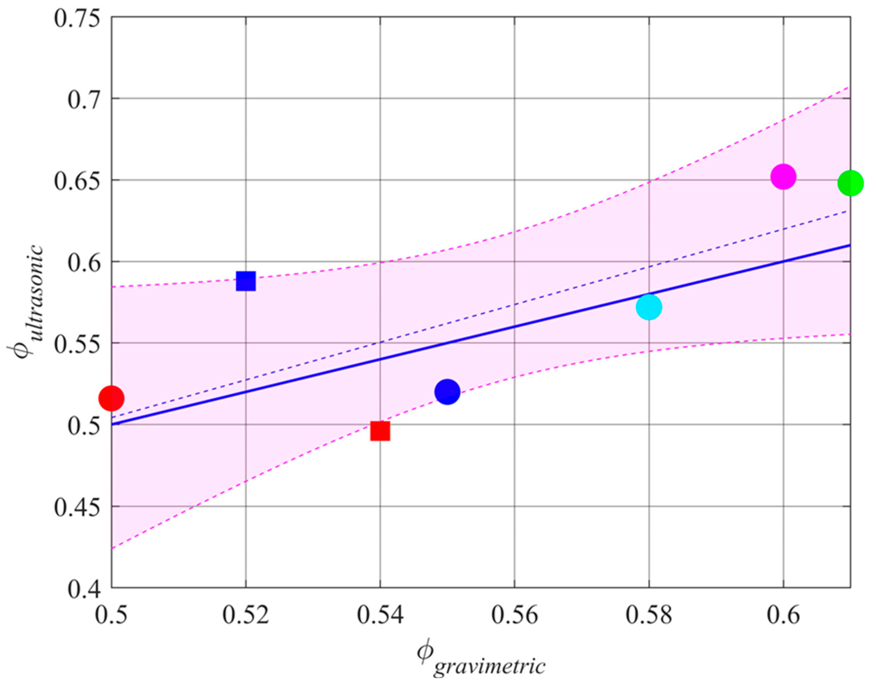
After the acoustic test, the samples were saturated for 4 days and weighted again. Porosity was determined using the gravimetric method [19] by comparing the saturated weight and oven-dried weight of the samples, giving porosity estimates of ϕgravimetric = 0.55, 0.50, 0.61, 0.60, 0.58, 0.52 and 0.54 for samples 1 to 7 respectively. The porosities estimated from ultrasonic measurements were ϕultrasonic = 0.52, 0.52, 0.65, 0.65, 0.57, 0.59 and 0.50 for samples 1 to 7 respectively, as shown in Figure 12.
The square root of the mean of the squares of the differences between ϕultrasonic and ϕgravimetric (the rmse) is 0.04. The variation of χ2 above its minimum at ϕultrasonic ± 0.04 gives a guide to the dependence on the other parameters, giving the standard deviation of estimates of α∞ as 0.08 and of σh as 0.30 mm. The estimates of rms surface height, σh, for the soil samples 1 to 4 are 0.00, 1.23, 1.53, and 2.10 mm, agreeing with the visual assessment of roughness in Figure 11. For the fifth soil sample an optical scan of the surface height was performed [20], giving a rms surface height variation of σh = 1.23 mm, and that estimated using ultrasound 1.62 mm. This ultrasound estimate is 1.3 of the 0.04 standard deviations above the optical estimate of σh, but the optical estimate can also be expected to contain uncertainties so the agreement is not unreasonable.
4. Discussion
It is relatively straight-forward to use reflections of ultrasound to measure porosity of samples of materials in the laboratory [21,22,23], but the intent of the current work is to design a readily useable technology for routine paddock-scale porosity estimation. This creates some challenges because the design must comprise a compact low-power rigid structure and allow for pasture cover and surface roughness.
The high-frequency regime for acoustic interactions with a porous material involves the porosity ϕ, the tortuosity α∞, and the angle of incidence θ [7]. There is no dependence on frequency, so measurements must be conducted at two or more angles of incidence θ to obtain two or more equations in the unknown ϕ and α∞. A system requiring a single transmitter/receiver pair to be moved from one angle to another is not viable for rapid sampling. Therefore, for specular reflections, at least two transmitter/reflector pairs are required. Ideally these are placed at identical distances from the ground so that the power reflected from a perfectly reflecting surface would be the same.
To operate in the high-frequency regime for porosity, the frequency needs to be well above 6 kHz. In the low ultrasound frequency range the loss of reflected signal due to scattering by surface roughness also takes a simple form [10]. The result is that the combination of porosity effects and roughness effects can be handled using a single 25 kHz frequency.
Penetration of pasture also appears to be adequate in the low ultrasound frequency range below about 30 kHz [13], but a model for scattering of ultrasound by pasture is required to interpret the reflections, which will be treated in a future article.
Given available transmitter and receiver elements, it is desirable to include multiple transmitter elements into a transmitter array and multiple receiver elements into a microphone array. The array design is a pragmatic choice based on compactness of the overall system and on providing sufficient flexibility in choosing angles of incidence. The result is arrays of diameter 100 mm, although this is a little arbitrary.
Pulsed ultrasound is used so that the reflected sound can be separated from sound travelling directly through the air from transmitter to receiver. Because of the directionality achieved by an array, and because of the directionality of the individual acoustic components, the intensity of the direct sound is not large, but would interfere significantly with the reflected signal.
Calibration of the transmitter/receiver pairs is discussed. It is straight-forward to point a transmitter array at a receiver array and obtain a combined transmitter/receiver gain, which is what is required in practice. The acoustic beam shape has also been measured for confirmation of expectations (this is not required for data interpretation and in deriving porosity).
The design has been tested on a limited number of soil samples in the laboratory and on bare agricultural soils. The result is that the average porosity estimated for each sample was within around 0.04 of the independently measured porosity value. This level of variation is consistent with uncertainties in setting the angle of incidence. Assumptions made in modelling the interaction of ultrasound with the rough surface no doubt also contribute. The 0.04 variation in porosity estimation is a very encouraging result, but the methodology needs to be tested on a much wider range of soil samples and with a range of pasture biomass cover. No allowance is currently made for larger scale “pugging” by animals, and soil pores partially filled with water will likely give a false impression of the overall soil porosity.
The measurements described were made with the transmitters and receivers fixed in space. For eventual operational applications the sensor platform will be moving. Even at a typical walking speed of 4.5 km h-1 (1.25 m s-1) successive measurements at around 30 ms intervals will have footprints which do not overlap. This means that regressions will need to be performed on each reflected pulse, and then estimated porosity values averaged if required. Given the low random noise levels this should not present a problem.
5. Conclusions
Directional ultrasonic transmitter and receiver arrays, operating at 25 kHz have been designed to quantify soil porosity. The method is based on simultaneous, multi-angle non-contact measurements of ultrasonic reflections from the soil, allowing soil porosity measurements in real time. A number of constraints are described, relating to the ultrasound scattering and to the required geometry of the sensor array placements. The resulting design is compact and relatively inexpensive, and capable of being mounted on a small farm vehicle. This results in a soil porosity monitoring method which has promising potential for operational use at paddock scales.
Data Availability Statement
The datasets presented in this article are not made available because the data are part of an ongoing study involving estimation of porosity of pasture-covered soils.
Acknowledgments
The authors are grateful to AgResearch for funding to support this research.
Author Contributions
Stuart Bradley: Conceptualization, Methodology, Software, Investigation, Validation, Writing- Original draft preparation. Chandra Ghimire: Funding acquisition, Project administration, Supervision, Visualization, Investigation, Data curation, Writing- Reviewing and Editing.
Conflict of Interest
There are no conflicts of interest.
References
- Doran, J.W.; Zeiss, M.R. Soil Health and Sustainability: Managing the Biotic Component of Soil Quality. Applied Soil Ecology 2000, 15, 3–11. [Google Scholar] [CrossRef]
- Lehmann, J.; Bossio, D.A.; Kögel-Knabner, I.; Rillig, M.C. The Concept and Future Prospects of Soil Health. Nat Rev Earth Environ 2020, 1, 544–553. [Google Scholar] [CrossRef] [PubMed]
- Shahane, A.A.; Shivay, Y.S. Soil Health and Its Improvement Through Novel Agronomic and Innovative Approaches. Frontiers in Agronomy 2021, 3. [Google Scholar] [CrossRef]
- Leclaire, P. Characterization of Porous Absorbent Materials. In Proceedings of the Acoustics 2012; Nantes, France., 2012; Vol. hal-00810634.
- Nimmo, J.R. Porosity and Pore Size Distribution. In Reference Module in Earth Systems and Environmental Sciences; Elsevier, 2013; p. B9780124095489052659 ISBN 978-0-12-409548-9. [CrossRef]
- Ghajar, S.; Tracy, B. Proximal Sensing in Grasslands and Pastures. Agriculture 2021, 11, 740. [Google Scholar] [CrossRef]
- Brennan, M.J.; To, W.M. Acoustic Properties of Rigid-Frame Porous Materials — an Engineering Perspective. Applied Acoustics 2001, 62, 793–811. [Google Scholar] [CrossRef]
- Salomons, E.M. Computational Atmospheric Acoustics; Springer Science & Business Media, 2001; ISBN 978-1-4020-0390-5. [CrossRef]
- Hawke, R.; McConchie, J. In Situ Measurement of Soil Moisture and Pore-Water Pressures in an ‘Incipient’ Landslide: Lake Tutira, New Zealand. Journal of Environmental Management 2011, 92, 266–274. [Google Scholar] [CrossRef] [PubMed]
- Medwin, H.; Clay, C.S. Fundamentals of Acoustical Oceanography; Applications of Modern Acoustics; Academic Press: London, 1997; ISBN 978-0-08-053216-5. [CrossRef]
- Govers, G.; Takken, I.; Helming, K. Soil Roughness and Overland Flow. Agronomie 2000, 20, 131–146. [Google Scholar] [CrossRef]
- Hannaway, D.B.; Evers, G.W.; Fales, S.L.; Hall, M.H.; Fransen, S.C.; Ball, D.M.; Johnson, S.W.; Jacob, I.H.; Chaney, M.; Lane, W.; et al. Perennial Ryegrass for Forage in the USA. In Ecology, Production, and Management of Lolium for Forage in the USA; John Wiley & Sons, Ltd, 1997; pp. 101–122 ISBN 978-0-89118-603-8. [CrossRef]
- Legg, M.; Bradley, S. Ultrasonic Proximal Sensing of Pasture Biomass. Remote Sensing 2019, 11, 2459. [Google Scholar] [CrossRef]
- Prabhu, K.M.M. Window Functions and Their Applications in Signal Processing; 1st edition. CRC Press: Singapore, 2013; ISBN 978-981-4463-08-9. [Google Scholar] [CrossRef]
- Born, M.; Wolf, E. Principles of Optics: 60th Anniversary Edition. Available online: https://www.cambridge.org/core/books/principles-of-optics/9D54D6FF0317074912CB285C3FF7341C (accessed on 22 June 2023).
- Cheon, Y.; Muschinski, A. Closed-Form Approximations for the Angle-of-Arrival Variance of Plane and Spherical Waves Propagating through Homogeneous and Isotropic Turbulence. J. Opt. Soc. Am. A 2007, 24, 415. [Google Scholar] [CrossRef] [PubMed]
- Jasiewicz, J.; Zwolinski, Z.; Mitasova, H.; Hengl, T. Geomorphometry for Geosciences; 2015; ISBN 978-83-7986-059-3.
- Thomsen, L.M.; Baartman, J.E.M.; Barneveld, R.J.; Starkloff, T.; Stolte, J. Soil Surface Roughness: Comparing Old and New Measuring Methods and Application in a Soil Erosion Model. SOIL 2015, 1, 399–410. [Google Scholar] [CrossRef]
- Klute, A. Methods of Soil Analysis, Part 1, Physical and Mineralogical Methods; Agronomy Monographs; 2nd ed.; American Society of Agronomy: Madison, Wisconsin, 1986; Vol. 9 (1). [CrossRef]
- Grundy, L.; Ghimire, C.; Snow, V. Characterisation of Soil Micro-Topography Using a Depth Camera. MethodsX 2020, 7, 101144. [Google Scholar] [CrossRef] [PubMed]
- Fellah, Z.E.A.; Berger, S.; Lauriks, W.; Depollier, C.; Aristégui, C.; Chapelon, J.-Y. Measuring the Porosity and the Tortuosity of Porous Materials via Reflected Waves at Oblique Incidence. The Journal of the Acoustical Society of America 2003, 113, 2424–2433. [Google Scholar] [CrossRef] [PubMed]
- Fellah, Z.E.A.; Berger, S.; Lauriks, W.; Depollier, C.; Fellah, M. Measuring the Porosity of Porous Materials Having a Rigid Frame via Reflected Waves: A Time Domain Analysis with Fractional Derivatives. Journal of Applied Physics 2003, 93, 296–303. [Google Scholar] [CrossRef]
- Fellah, Z.E.A.; Mitri, F.G.; Depollier, C.; Berger, S.; Lauriks, W.; Chapelon, J.Y. Characterization of Porous Materials with a Rigid Frame via Reflected Waves. J. Appl. Phys. 2003, 94, 7914. [Google Scholar] [CrossRef]
Figure 1.
The geometry of the placement of transmitter and receiver pairs. The transmitter unit and receiver unit are both a distance r0 from the target area on the ground. The angle of incidence is θ and the receiver subtends an angle 2Δθ at the transmitter. A horizontal direct path of length 2r0sinθ is shown. The image of the receiver is referred to in Section 2.4.
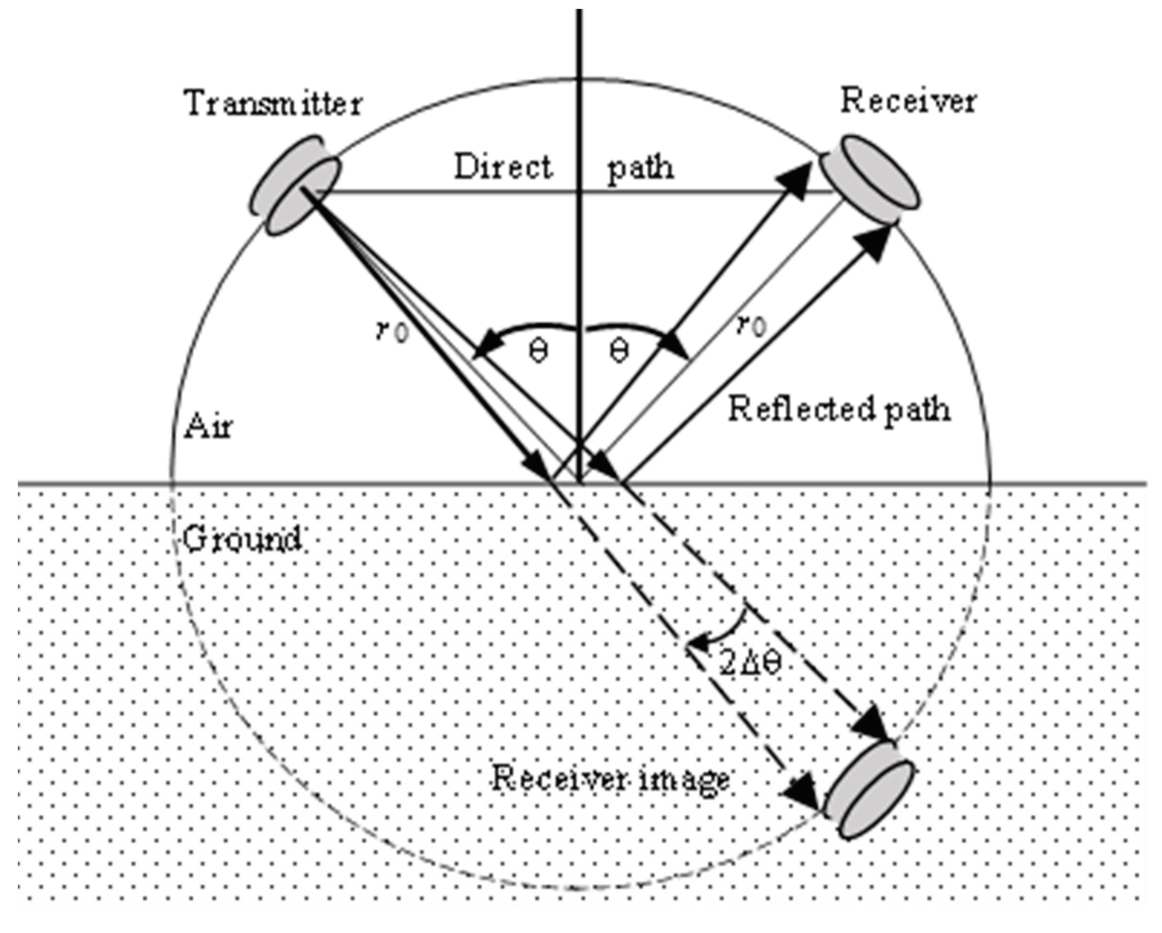
Figure 2.
Frequency dependencies: fc with α∞ = 1.35, ϕ = 0.65, and σ = 1 x 10⁵ Pa s m-2 (red line); fV with w = 4 mm (green line); exp(-g2/2) with σh = 2 mm and θ = 0° (blue curve); and exp(-g2/2) with σh = 2 mm and θ = 60° (magenta curve). Central frequencies of typical transmitter elements are 25 kHz (solid black line) and 40 kHz (dashed black line).
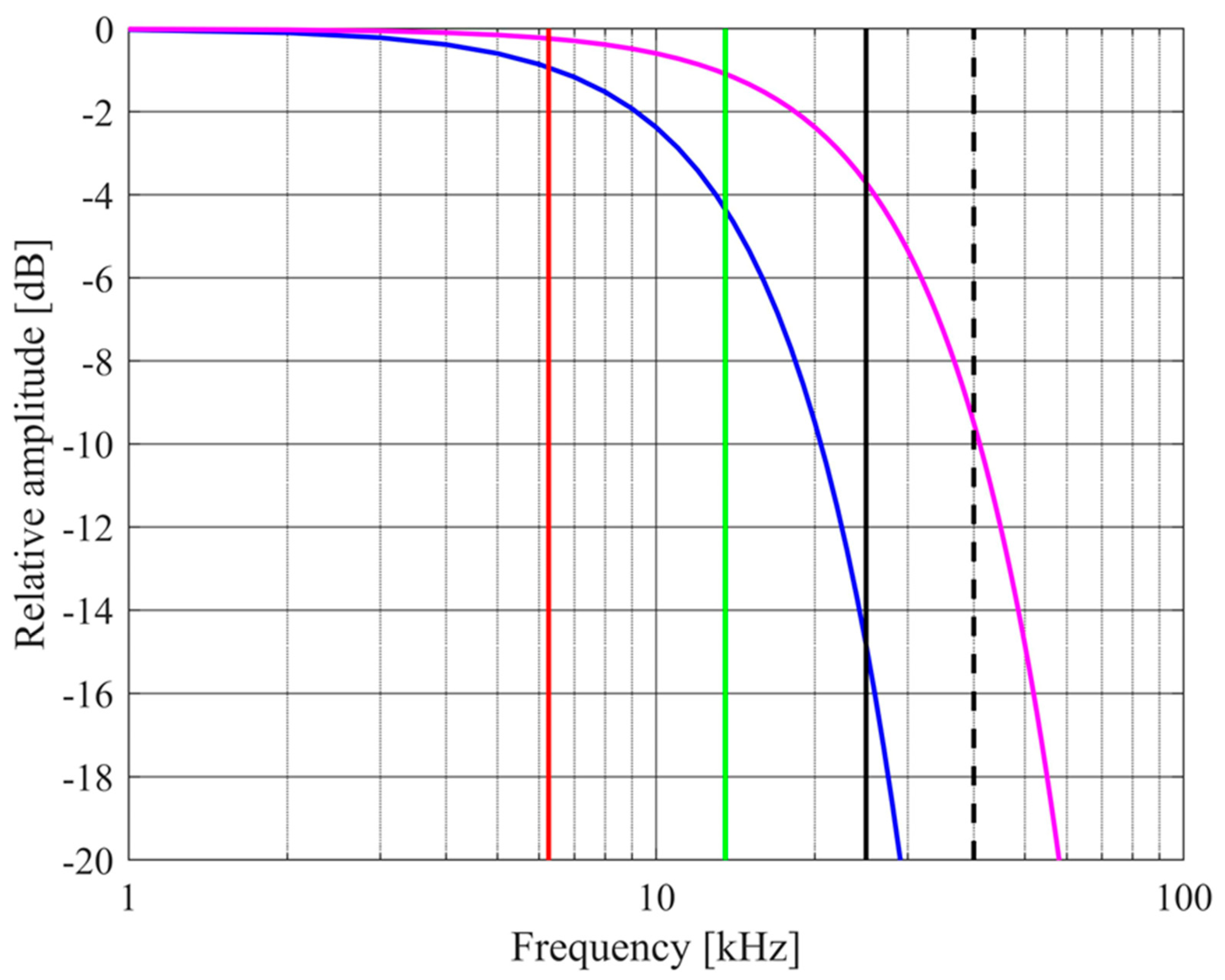
Figure 3.
The normalized measured signal (red curve) from a soil sample at θ = 30° (upper plot) and at θ = 52° (lower plot), together with the predicted onset of the direct pulse arrivals (green lines) and the reflected pulse arrivals (blue lines). A small reflection from the supporting frame is also evident ahead of the ground reflection in the θ = 30° case.
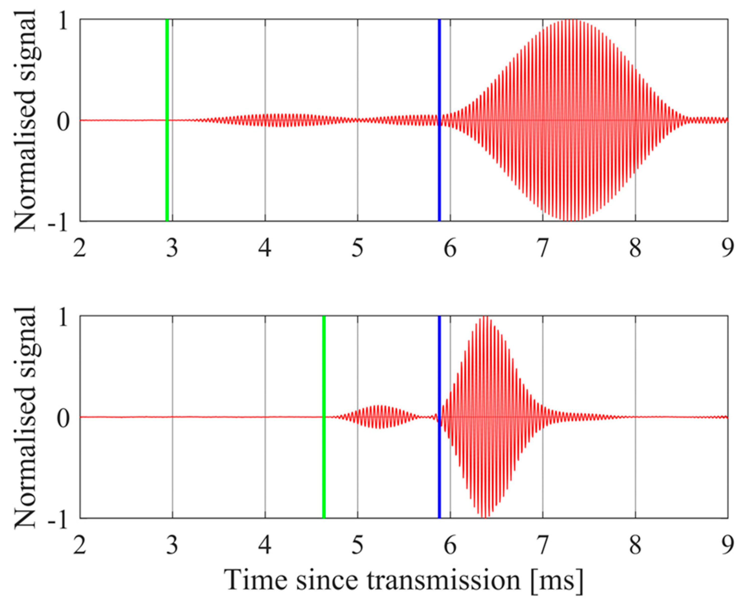
Figure 4.
The decrease in amplitude across a receiver of radius a, given a transmitter also of radius a (blue curve) and at the chosen array radius of 38 mm (red line). The transmitted frequency is fT = 25 kHz and the range is 2r0 = 2000 mm.
Figure 4.
The decrease in amplitude across a receiver of radius a, given a transmitter also of radius a (blue curve) and at the chosen array radius of 38 mm (red line). The transmitted frequency is fT = 25 kHz and the range is 2r0 = 2000 mm.
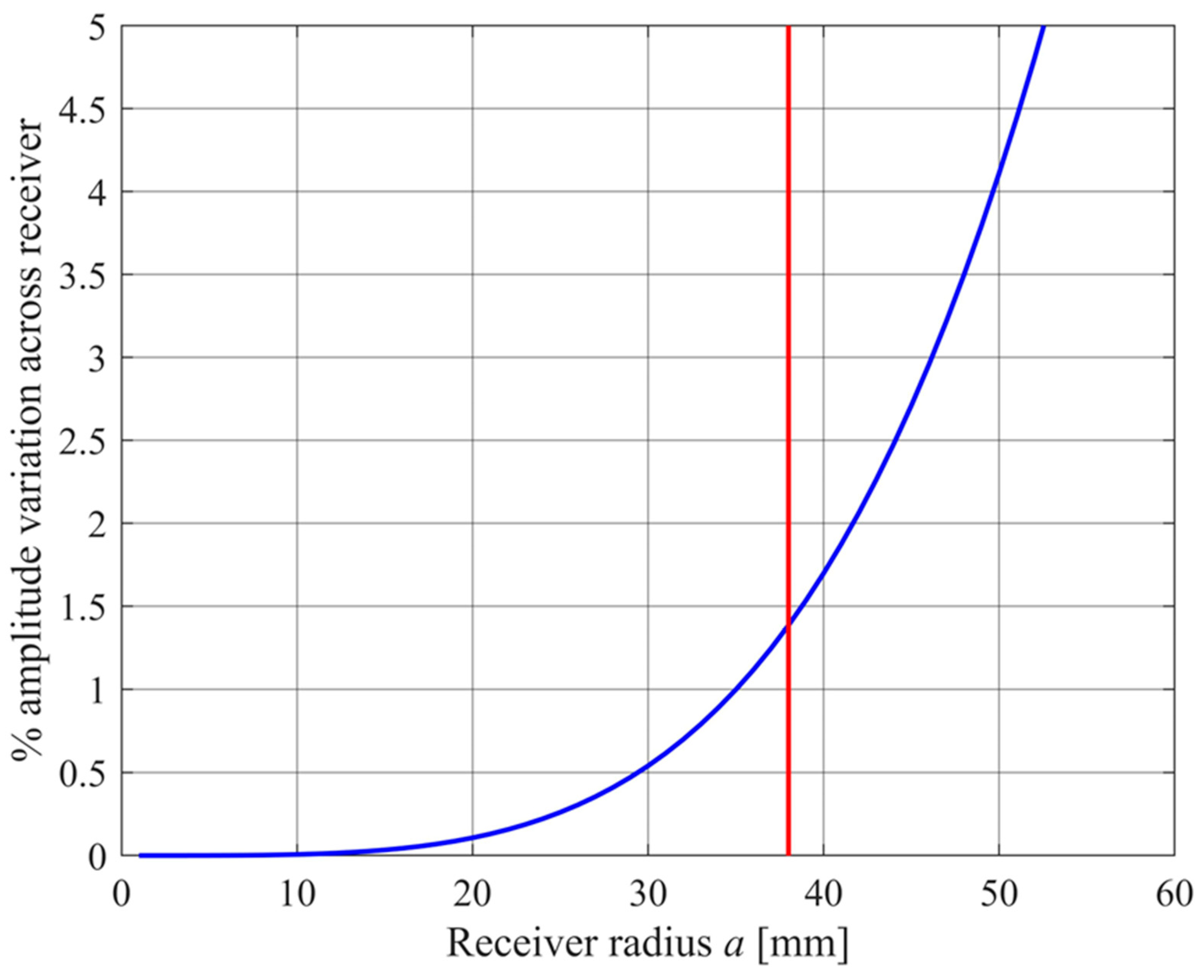
Figure 5.
Predicted plane wave reflection coefficient R for a porous surface with α∞ = 1.35, ϕ = 0.65 (blue curve) and for α∞ = 1.35, ϕ = 0.85 (red curve).
Figure 5.
Predicted plane wave reflection coefficient R for a porous surface with α∞ = 1.35, ϕ = 0.65 (blue curve) and for α∞ = 1.35, ϕ = 0.85 (red curve).
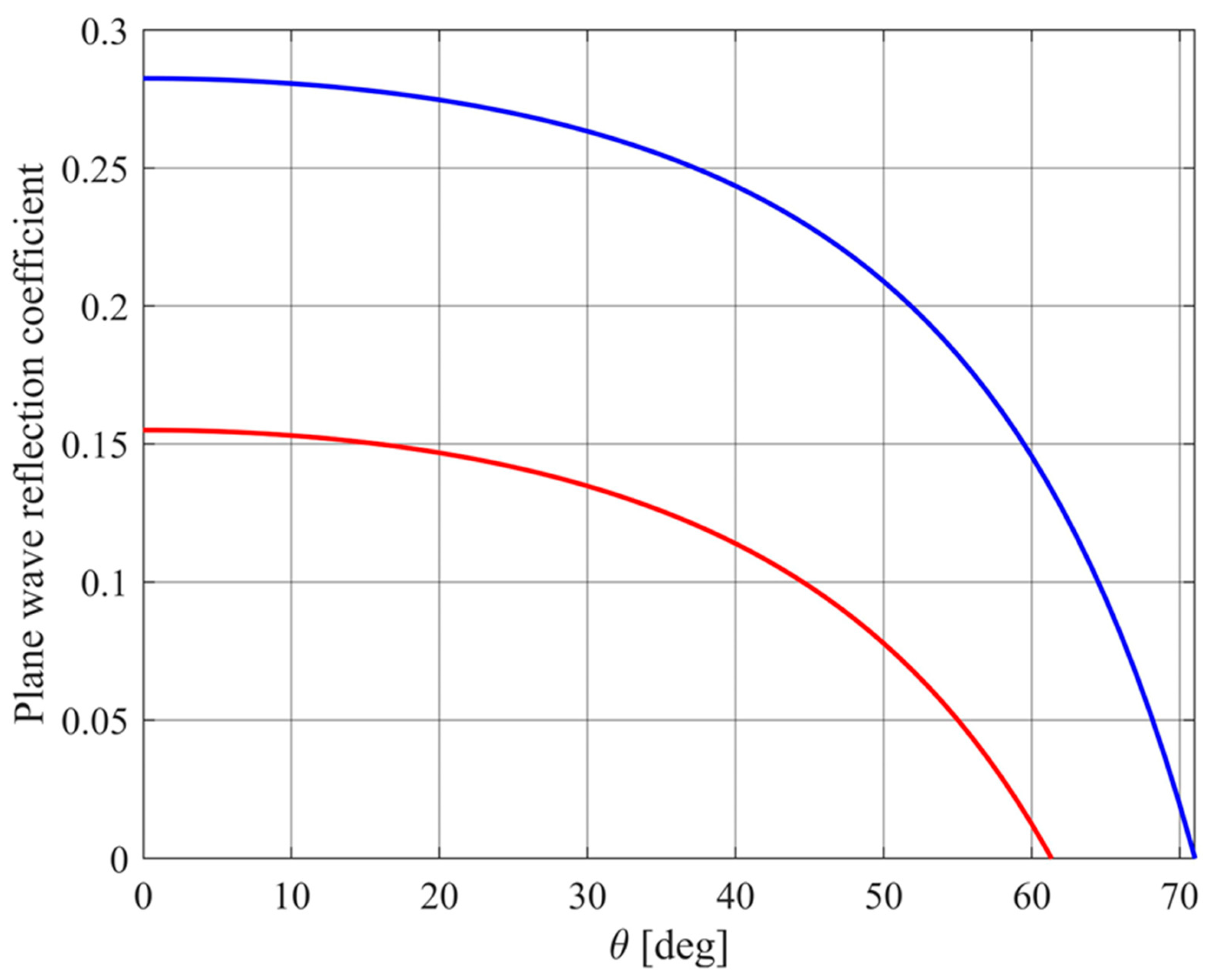
Figure 6.
The SPL produced by a single 250ST/R160 transmitter element at a distance of rspec = 0.3 m when driven by a sinusoidal signal of Vspec = 10Vrms.
Figure 6.
The SPL produced by a single 250ST/R160 transmitter element at a distance of rspec = 0.3 m when driven by a sinusoidal signal of Vspec = 10Vrms.
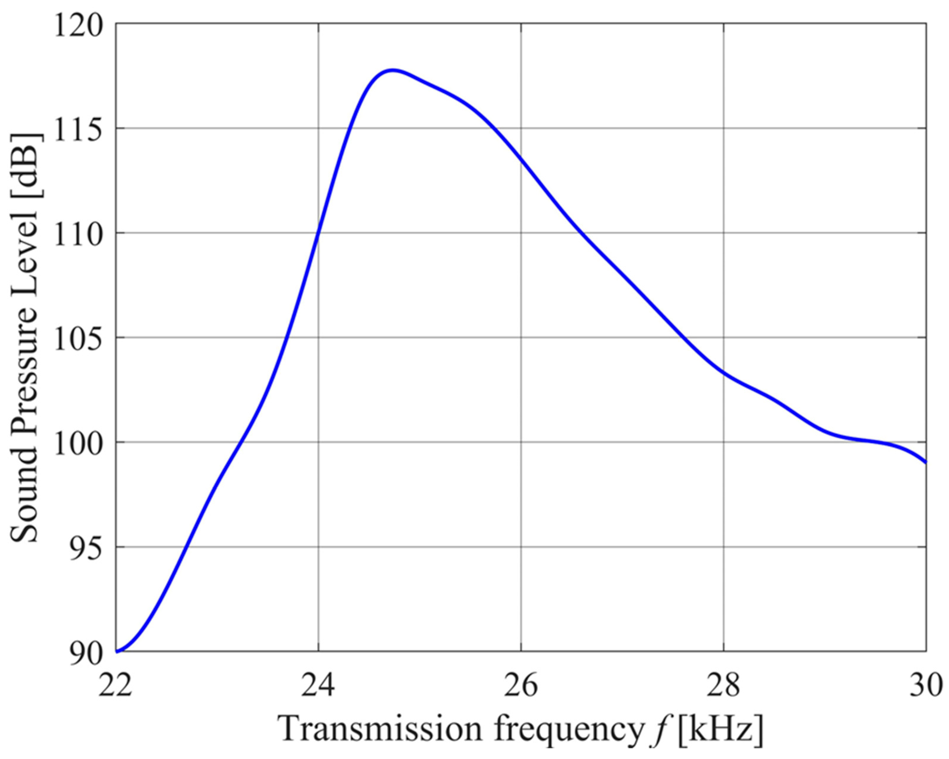
Figure 7.
The normalized polar response, in dB, of a single 250ST160 transmitter element at 25 kHz.
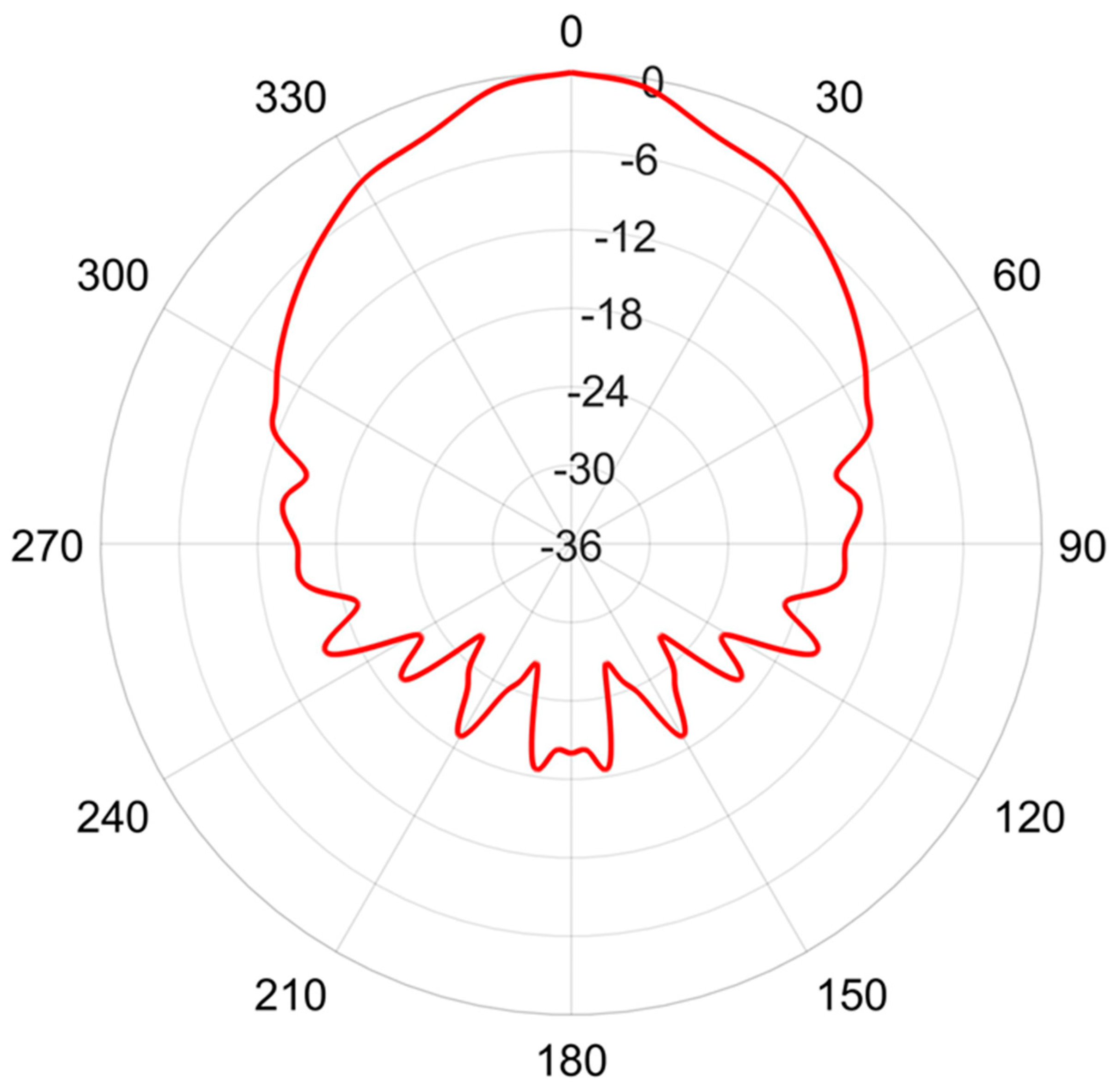
Figure 8.
The transmitter circuit board. The large circular items are the transmitter elements.
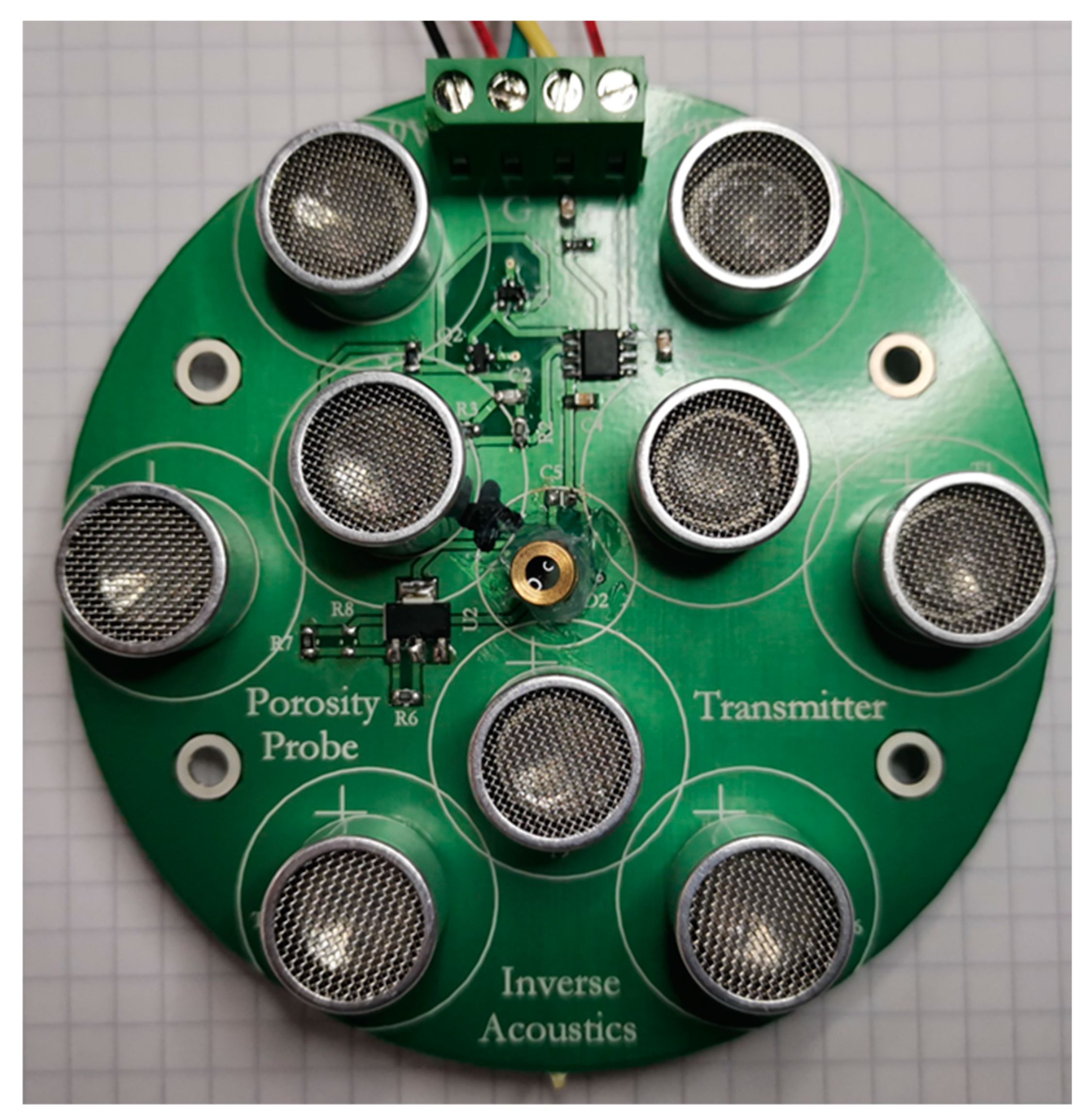
Figure 9.
The receiver circuit board. The small circular black items are the ultrasonic receiver elements and the central brass tube is a laser diode.
Figure 9.
The receiver circuit board. The small circular black items are the ultrasonic receiver elements and the central brass tube is a laser diode.
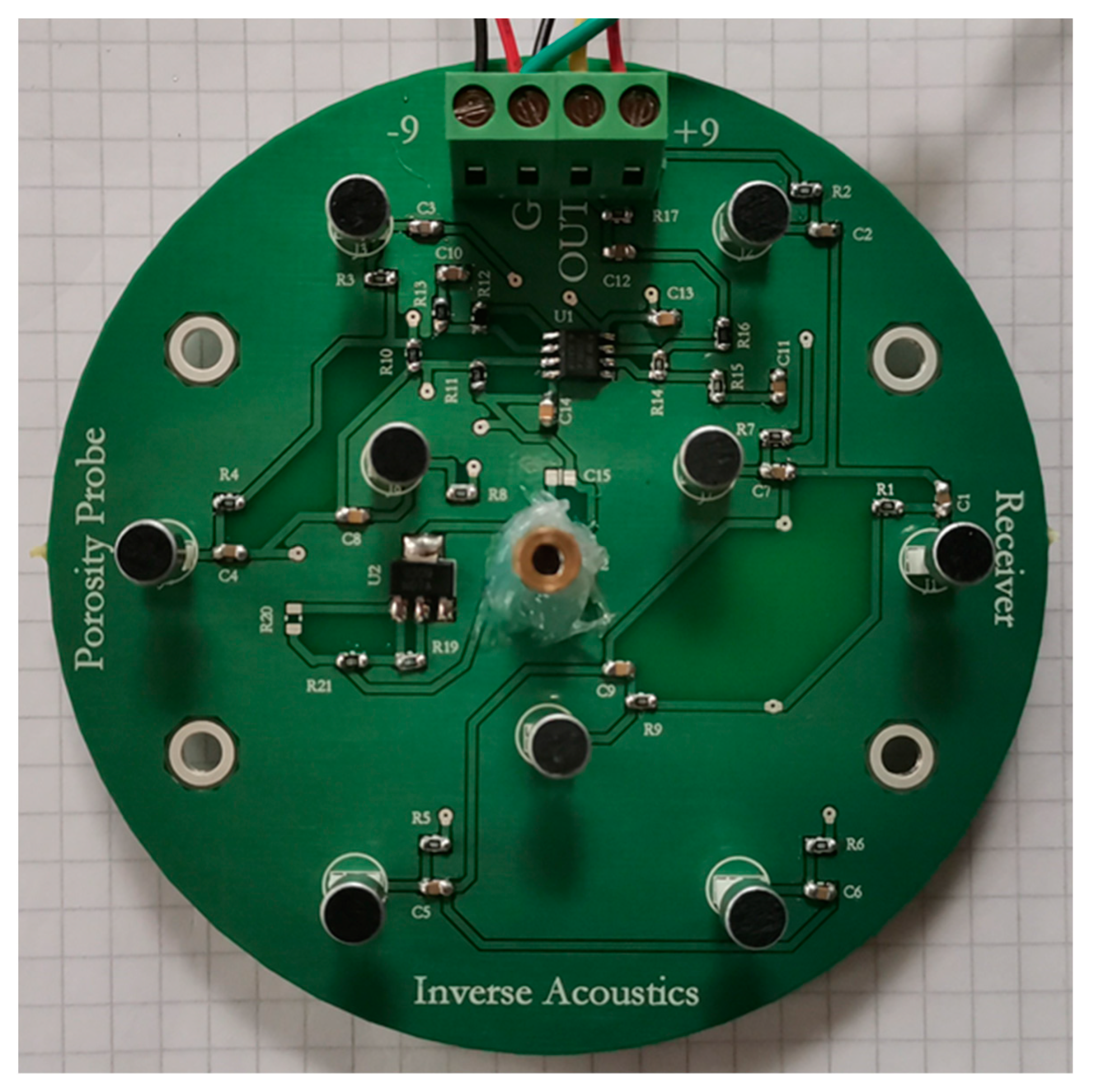
Figure 10.
Results of measured system gain G(Δθ) for 3 transmitter-receiver pairs (red circles, green squares, and blue triangles). Also shown is the Airy pattern (8) with a = 51 mm and scale factor G0 = 9.1 (magenta curve).
Figure 10.
Results of measured system gain G(Δθ) for 3 transmitter-receiver pairs (red circles, green squares, and blue triangles). Also shown is the Airy pattern (8) with a = 51 mm and scale factor G0 = 9.1 (magenta curve).
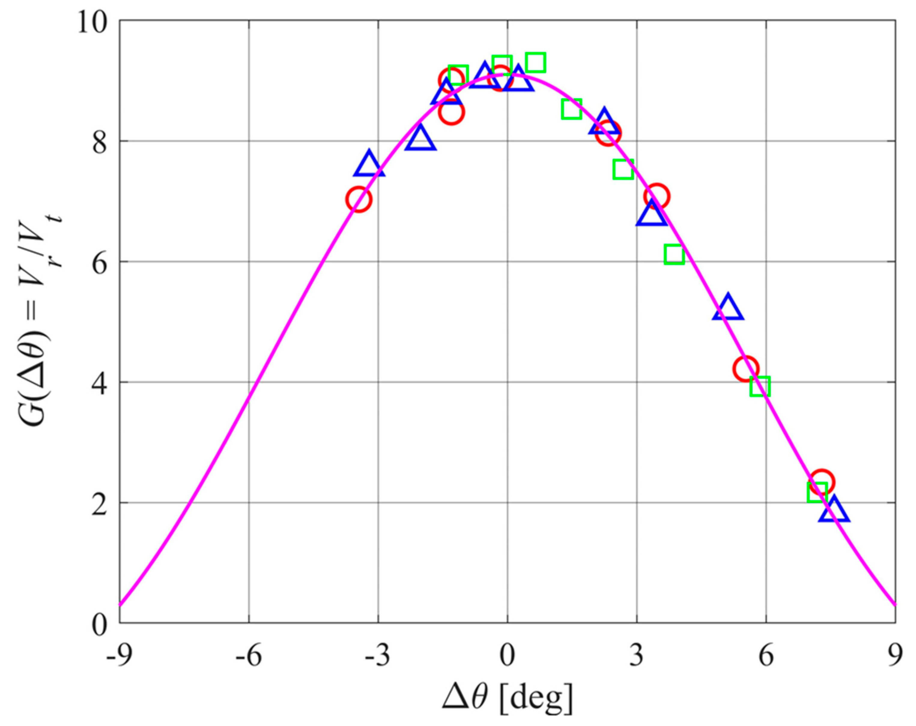
Figure 11.
Soil samples 1 to 4 (numbering from the left).
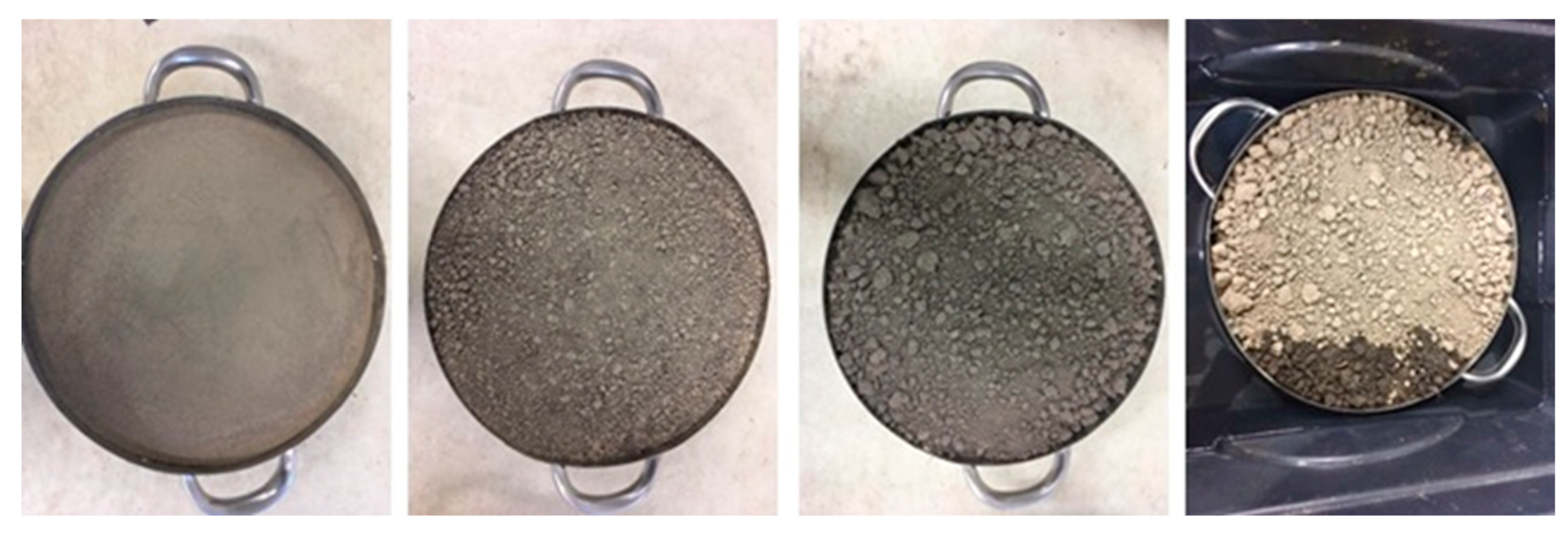
Figure 12.
Results of soil porosity estimation compared with the porosity values independently estimated from the gravimetric method. The result for laboratory soil samples are shown as circles (soil 1 blue, soil 2 red, soil 3 green, soil 4 magenta, soil 5 cyan), those from bare field samples by squares (soil 6 blue, soil 7 red). The least squares regression is shown as a dashed blue line and 1:1 as a solid blue line. The magenta shaded area is the 95% confidence bounds.
Disclaimer/Publisher’s Note: The statements, opinions and data contained in all publications are solely those of the individual author(s) and contributor(s) and not of MDPI and/or the editor(s). MDPI and/or the editor(s) disclaim responsibility for any injury to people or property resulting from any ideas, methods, instructions or products referred to in the content. |
© 2024 by the authors. Licensee MDPI, Basel, Switzerland. This article is an open access article distributed under the terms and conditions of the Creative Commons Attribution (CC BY) license (http://creativecommons.org/licenses/by/4.0/).
Copyright: This open access article is published under a Creative Commons CC BY 4.0 license, which permit the free download, distribution, and reuse, provided that the author and preprint are cited in any reuse.


