
Submitted:
29 February 2024
Posted:
01 March 2024
You are already at the latest version
Abstract
This paper investigates portfolio optimization methodologies and short-term investment strate-gies in the context of the cryptocurrency market, focusing on ten major cryptocurrencies from January 2020 to November 2023. We employ high frequency data and utilize the Kurtosis Mini-mization methodology, alongside other optimization strategies, to construct and evaluate port-folios under different rebalancing frequencies. The empirical analysis reveals that cryptocurren-cies exhibit significant volatility, skewness, and kurtosis, necessitating sophisticated portfolio management techniques. We find that the Kurtosis Minimization methodology consistently outperforms other optimization strategies, delivering optimal returns to investors, particularly in shorter-term investment horizons. We demonstrate the diversification benefits of integrating cryptocurrencies into multi-asset portfolios and emphasize the importance of regular portfolio rebalancing in the volatile cryptocurrency market. Our findings offer insights for portfolio man-agers and investors seeking to optimize their investment outcomes in the cryptocurrency market, highlighting the importance of risk management, diversification, and dynamic portfolio man-agement strategies.
Keywords:
Portfolio Optimization
; Sharpes
; Kurtosis minimization
; High-Frequency
; Rebalancing frequency
; Diversification
; Short-term investment strategy
1. Introduction
Cryptocurrencies are reshaping the financial landscape, poised to revolutionize the global financial system (Rajharia, 2023). These digital assets garner attention from policymakers, investors, and academics as a burgeoning alternative asset class (Jana, 2024), exhibiting unprecedented growth and establishing a significant international foothold (Subramoney et al., 2023). Consequently, interest in their impact on traditional financial markets is burgeoning (Krishna, 2023).
Cryptocurrency, characterized as a digital or virtual currency devoid of traditional backing like precious metals or commodities (Khan, 2022), presents a unique challenge in understanding inter- and intra-asset dependencies among key financial variables (Zhang, 2024). A comprehensive understanding of cryptocurrencies is imperative to expedite their broader adoption within the financial ecosystem (Shahzad, 2024), particularly given their dynamic role within the evolving financial landscape (Wang, 2024).
The rapid expansion of cryptocurrencies unfolds amidst an evolving regulatory framework, necessitating a nuanced approach to investment strategies. Regulatory considerations, encompassing consumer protection, financial stability, and taxation, loom large in the cryptocurrency space.
The genesis of cryptocurrencies traces back to Bitcoin's emergence in 2009, catalyzing a tumultuous evolution of the cryptocurrency market (ElBahrawy et al., 2017). Originally conceived to cater to the unbanked, reduce costs and energy consumption, and eliminate financial intermediaries (McMorrow & Esfahani, 2021), cryptocurrencies have morphed into a distinct species within the financial instrument ecosystem.
Characterized by decentralization, volatility, and high risk-reward potential, cryptocurrencies have ascended in global financial significance, attracting investors seeking diversification and short-term gains (Mungo et al., 2023). Consequently, understanding interdependencies in cryptocurrency markets is indispensable for informed decision-making (Alipour & Charandabi, 2023).
Effective portfolio management emerges as pivotal in mitigating risks and maximizing returns in cryptocurrency investments. The dynamic nature of cryptocurrencies necessitates a thorough analysis to inform policymakers and regulatory bodies of their evolving role as investment assets. Cryptocurrencies offer potential avenues for risk diversification and portfolio optimization (Araujo et al., 2023), improving the risk-return trade-off and enhancing portfolio efficiency (Trimborn et al., 2019).
The study's novelty lies in its utilization of the top ten cryptocurrencies based on market capitalization. Our objective is to investigate the effectiveness of utilizing kurtosis in the portfolio construction framework, specifically by minimizing the kurtosis of the portfolio. This approach will be compared with the traditional Sharpe's maximization technique to determine which method performs better in the realm of cryptocurrency.
Furthermore, we implemented four short-term strategies (half-week, one-week, four-week, and eight-week) for portfolio construction. Each strategy was tested using three different methodologies: naive portfolio construction, Sharpe-maximization, and kurtosis-minimization. This comprehensive approach allows us to assess which short-term strategy aligns best with the volatile nature of cryptocurrencies.
To evaluate the performance of each portfolio, we considered both holding period returns and annualized returns. Statistical analysis techniques were then applied to the data to identify significant trends or patterns. This systematic analysis provides insights into the efficacy of different portfolio construction methods and short-term strategies within the cryptocurrency market.
2. Literature Review
The literature on cryptocurrency portfolio management strategies provides insights into various methodologies and their implications in cryptocurrency markets. Gupta et al. (2022) explore reducing portfolio risk using cryptocurrencies, highlighting associated challenges. Silva et al. (2022) critically evaluate cryptocurrency trading algorithms, identifying areas for further exploration. Lorenzo & Arroyo (2023) compare risk-based portfolio allocation on crypto asset subsets, enriching portfolio management literature. Symitsi & Chalvatzis (2019) quantify economic gains achievable through cryptocurrency portfolio strategies.
Research explores interlinkages between major cryptocurrencies (Yousaf & Ali, 2020), portfolio diversification in emerging markets (Letho et al., 2022), and volatility's impact on cryptocurrency investment (Zaretta & Pangestuti, 2023), offering insights into market dynamics.
The evolving regulatory landscape significantly influences investment strategies, impacting safety perceptions, risk characteristics, and market dynamics. Conlon et al. (2020) illustrate how regulatory developments during the COVID-19 pandemic affect cryptocurrencies' role as a safe haven for equity markets. Sukumaran et al. (2022) focus on regulatory developments in specific jurisdictions, while Waspada et al. (2022) stress regulation's importance in managing risks associated with emerging crypto assets.
Ethical considerations in cryptocurrency investments are crucial for responsible practices. Bagus & Horra (2021) undertake an ethical assessment of cryptocurrencies, highlighting considerations associated with investment decisions. Insights from behavioral finance literature aid in understanding investors' psychological factors and decision-making in cryptocurrency investments (Ballis & Verousis, 2022; Zhao & Zhang, 2021; Choi & Feinberg, 2022).
Optimization methodologies like Naive portfolio, Sharpe-maximization, and Kurtosis-minimization are pivotal for cryptocurrency portfolio testing (Hanif et al., 2023). Recent research challenges outperforming the Naive portfolio approach under the Sharpe ratio criteria (Ma et al., 2020). Sharpe-maximization aims at maximizing risk-adjusted returns (Dabbous et al., 2022), while Kurtosis-minimization aims to mitigate extreme tail risk and volatility (Susilo et al., 2020).
Short-term strategies and optimization methodologies are crucial for navigating cryptocurrency market dynamics. Mean-variance optimization techniques offer insights into short-term portfolio management (Inci & Lagasse, 2019), and robust risk management strategies mitigate short-term volatility (Kozlovskyi et al., 2022). High-frequency data analysis aids in understanding trading patterns, market efficiency, and volatility co-movements in cryptocurrency markets (Petukhina et al., 2020; Zhang et al., 2020).
Analysis of relationships and dependencies between cryptocurrencies through methodologies like logarithmic returns and correlation matrices aids in portfolio diversification and risk management strategies (Scagliarini et al., 2022; Plerou et al., 2002).
Testing strategies across different time horizons captures distinct aspects of their performance, emphasizing the importance of considering different time horizons in strategy testing (Nasir & Wahab, 2022). Additionally, the buy-and-hold strategy exhibits variability in performance in cryptocurrency markets compared to other trading rules (Adrianus & Soekarno, 2018).
The existing literature on cryptocurrency portfolio management strategies offers a comprehensive understanding of digital assets within the global financial system. Effective portfolio management strategies are crucial as cryptocurrencies disrupt traditional financial markets. The studies reviewed underscore the importance of considering interdependencies among major cryptocurrencies, volatility's impact on investment decisions, and the significance of short-term strategies in navigating market dynamics.
Our study addresses a gap in the existing literature by examining the effectiveness of various portfolio optimization methodologies in short-term investments using a selection of ten cryptocurrencies. While previous studies have investigated portfolio management strategies and optimization techniques in cryptocurrency markets, we have not specifically focused on comparing different short-term investment strategies and their corresponding portfolio optimization methods. We aim to fill this gap by exploring which short-term investment strategy would be most suitable for investors in the cryptocurrency market and, within each strategy, identifying the optimal portfolio optimization approach. Through this analysis, we seek to provide valuable insights for investors looking to optimize their cryptocurrency portfolios for short-term gains.
3. Empirical Analysis
3.1. Data and Methodology
The hourly closing prices of the top ten cryptocurrencies by market capitalization—Bitcoin, Cardano, Chain-link, Dogecoin, Ethereum, Litecoin, Ripple, Tron, Tether and USD coin—are used to conduct this study. The data used for the study ranges from January 1st 2020 to 30th November 2023. All the data used for the analysis were downloaded from CoinMarketCap (https://coinmarketcap.com/coins/). The reason for choosing the period is to incorporate the effects post COVID-19 period.
Market capitalization serves as a vital metric for assessing the value and size of a cryptocurrency (Liu et al., 2022). Unlike individual cryptocurrency prices, which may not reflect the total value accurately, market capitalization provides a more comprehensive measure, allowing for comparisons with other cryptocurrencies. This concept mirrors the stock market, where market capitalization is calculated by multiplying the current stock price by the total number of shares outstanding. In the cryptocurrency realm, market capitalization is determined by multiplying the circulating supply (the number of coins available to the public) by the current price. Due to its significance, market capitalization is often a primary criterion for selecting cryptocurrencies. However, it should also be considered independently during portfolio optimization to ensure a well-rounded approach for practitioners.
The empirical analysis employs hourly returns due to their stronger kurtosis and their practical application in short-term strategic asset allocation. Table 1 presents the main summary statistics for the cryptocurrency hourly return dataset, revealing well-known stylized facts such as negative skewness and positive excess kurtosis typically observed in financial assets.
Nine out of ten hourly average returns from all cryptocurrencies display positive values, indicating that all currencies, except USD coin, gained value over the analyzed period. However, these averages hover close to 0%, with the lowest positive return recorded by Tether and the only negative return observed with USD coin. Ripple boasts the highest hourly median return at 0.015%, alongside the largest range of 45.65%.
The median and mean values for the sample analyzed are nearly identical, differing by less than 0.02%. Skewness, a measure of data distribution symmetry, varies among the cryptocurrencies, with Bitcoin, Tron, and USD coin exhibiting near symmetry, while Cardano, Litecoin, and Ripple display high skewness toward the lower tail.
Volatility, assessed through standard deviation and coefficient of variation, remains high across all cryptocurrencies, with coefficient of variation absolute values ranging from 114.18 (Bitcoin) to 23,808.26 (Tether). None of the currencies exhibit normality at a 99% confidence level according to the Jarque-Bera test, as indicated by consistently low p-values (< 0.01). Additionally, all cryptocurrencies demonstrate high kurtosis, with values ranging from 18.29 (Ethereum) to 2185.35 (USD coin).
The combination of high volatility, skewness, and kurtosis in the majority of currencies underscores the need for a methodology allowing investors to understand currency behavior and formulate improved portfolios that actively perform better by controlling factors such as kurtosis.
We start by calculating the returns through the log difference of consecutive hourly closing prices of cryptocurrencies, following the method described by Akyildirim et al. (2021). This calculation follows the equation:
𝑅ₙ = (𝐼𝑛 𝐶𝑃ₙ − 𝐼𝑛 𝐶𝑃₍ₙ₋₁₎) × 100
In this equation, Rₙ denotes returns on an nth hour in percentage; 𝐶𝑃ₙ denotes closing price on an nth hour; 𝐶𝑃₍ₙ₋₁₎ denotes closing price on the previous trading hour ; and In is a natural log.
After calculating the logarithmic returns, we construct the correlation matrix for its crucial role in portfolio management. It helps us understand the relationships between different assets within a portfolio, crucial for diversification and risk management (Sukumaran et al., 2015). Accurate estimation of correlations is essential for constructing well-diversified portfolios (Sukumaran et al., 2015) and controlling for the properties of the market factor included in a correlation matrix of stocks, vital for effective portfolio management (Eom et al., 2015).
Secondly, the correlation matrix filters out random and systemic co-movements in constructing portfolios, improving risk profiles (Zema et al., 2021). It enables capturing conditional volatility and correlation for forecasting future variance-covariance matrices between assets for optimal portfolio construction (Razak, 2023). The correlation matrix is a fundamental component in portfolio optimization models, and its accurate estimation is crucial for their effectiveness (Tola et al., 2008).
The following six steps generate the correlation matrix:
Step 1. Calculating Variance: The variance, a measure of dispersion, is computed using the formula:
where x represents each variable in the database and n is the sample size.
Step 2. Computing Covariance: Covariance, a measure of dispersion between two variables, is determined by:
where denote pairs of variables, and is the sample size.
Step 3. Generating Variance-Covariance Matrix (mxm): The variance-covariance matrix is a square matrix of size (mxm) obtained by mapping the covariances of each pair of variables in the database. Variances are placed on the diagonal:
where is the number of variables.
Step 4. Calculating Correlation: Correlation between two variables is determined by dividing their covariance by the product of their standard deviations:
Where : Standard deviation of the variable,
Step 5. Generating Correlation Matrix (mxm): The correlation matrix is a square matrix of size (mxm) that maps the correlation of each pair of variables. It contains a diagonal of 1:
Step 6. Calculating Portfolio Variance: Portfolio variance, a measure of returns dispersion, is computed by multiplying the transposed vector of weights by the variance-covariance matrix, then by the vector of weights:
where is the vector of weights, is the transposed vector of weights, : is the variance-covariance matrix and number of assets in the portfolio.
Figure 1 depicts the correlation matrix, showcasing that a few cryptocurrencies in the study exhibit notable correlation levels. However, literature suggests that these high correlations may not significantly impact portfolio optimization. Antonakakis et al. (2019) found substantial correlation among Bitcoin, Ripple, and Litecoin, yet these assets remain relatively isolated from traditional financial instruments, suggesting their potential for diversifying portfolios and implying that high correlations among cryptocurrencies may not hinder diversification efforts. Similarly, Tzouvanas et al. (2020) identified cryptocurrencies as promising assets for a well-diversified portfolio, particularly for short-term investments. This underscores that, despite pronounced correlations among cryptocurrencies, they may not undermine the diversification benefits.
The study maintains its validity by including high-risk portfolios consisting solely of risky assets, aimed at maximizing returns through diverse strategies. However, mitigating risk by incorporating assets with negative correlations poses a challenge with cryptocurrencies, especially considering their tendency to mirror the price and return behavior of Bitcoin (Ji et al., 2019). Consequently, crafting a profitable cryptocurrency portfolio requires optimization. This process may pursue objectives such as maximizing the return-to-risk ratio, achieving maximum returns, or minimizing risk exposure.
After examining the correlation matrix, the next step is to construct a naive portfolio. In a naive portfolio, we allocate a fraction of 1/N of wealth to each of the N assets available for investment, following the naive rule. This approach commonly recommends the '1/N' allocation as a reference portfolio (DeMiguel et al., 2011). In this study, we assigned 10% to each of the 10 assets in the portfolio. We conducted empirical investigations employing two distinct portfolios: one utilizing the Sharpe-maximization methodology, and the other employing Kurtosis minimization methodology.
Initially, for a T-period-long dataset of returns, we estimated the input parameters necessary for computing optimal portfolio weights according to the two strategies. Subsequent periods, expressed in weeks, were utilized to assess the portfolio performance over the following W periods, with W dictated by the applied rebalancing frequency. Throughout these W periods, we implemented a buy-and-hold approach, more pragmatic for real-world investors than a constant mixed approach. The process iterated by shifting the estimation window forward by W periods and recalculating the optimal portfolio weights. This iterative approach allowed for accumulating returns for subsequent W periods while discarding an equivalent number of earliest returns. This process repeated until reaching the end of the dataset, ensuring comprehensive evaluation and optimization of the portfolios.
3.2. Sharpe-Maximization Methodology Portfolio
Constructing a portfolio that maximizes the Sharpe ratio offers numerous advantages within portfolio management. Investors utilize the Sharpe ratio, a crucial metric for evaluating investment performance as it assesses the risk-adjusted return of a portfolio. According to Siegel & Woodgate (2007), under appropriate conditions, portfolios that maximize the Sharpe ratio tend to become more diversified, indicating that maximizing the Sharpe ratio can enhance portfolio diversification.
Portfolio analysts widely employ the Sharpe-maximization methodology in portfolio analysis, as it assesses the opportunity cost of investing in a particular portfolio relative to the Risk-Free Asset.
In this study, we utilized the 28-day T-bill as a reference. To implement this methodology, we utilized rolling averages to smoothen the highly volatile database of prices and returns. We determined this smoothing process based on the time period chosen for each strategy.
where represent the expected return of portfolio, denotes the Risk free rate and indicates Standard deviation of the portfolio shown as
We adjusted the annual risk-free rate to match the frequency of the rebalancing period, ensuring consistency and accuracy in our calculations.
It's crucial to emphasize that whenever a negative Sharpe Ratio emerged—meaning that the return of the Risk-Free Asset surpassed that of the portfolio in that specific period—we opted to use the naive portfolio weights. In other words, we conducted rebalancing in every period without exception.
3.3. Kurtosis Minimization Methodology Portfolio
The Kurtosis methodology involves utilizing a descriptive statistic known as kurtosis, which measures how data disperse between a distribution's center and tails. Larger values of kurtosis suggest that a data distribution may have "heavy" tails, meaning they are thickly concentrated with observations or have long tails with extreme observations (Green, Manski, Hansen, & Broatch, 2023). This measurement is crucial for assessing dispersion or risk in financial assets.
In this methodology, the portfolio undergoes a process of optimization. This optimization entails searching for the lowest dispersion for each rebalancing period by selecting weights of the cryptocurrencies that minimize their kurtosis.
where, : kurtosis of the variable A normally distributed sample will have a kurtosis close to 3.
In the Pearson's kurtosis model, the kurtosis minimization methodology aims to regulate the kurtosis of the portfolio's assets by assigning lower weights to assets with higher kurtosis and vice versa. This calculation is performed during each rebalancing period to ensure the lowest possible kurtosis is achieved whenever currencies are traded.
Similar to the Sharpe maximization methodology, the same considerations and calculations were applied in this methodology. Rolling averages were utilized to smooth the highly volatile database of prices and returns, with the smoothing period determined by the strategy's timeframe. These rolled averages were then used to determine the portfolio weights that would result in the lowest possible kurtosis in each period. Subsequently, these weights were utilized in the subsequent holding period.
The formula for calculating the Kurtosis Minimization Portfolio Return is as follows:
represents the weight of asset n calculated with Kurtosis minimization in period t. denotes the return of asset n in period t+1.
where, : Sum of inverses of the kurtosis of all the variables in a portfolio.
The formula 11 ensures that the asset with the highest kurtosis receives the least weight of investment, while assets with lower kurtosis are assigned higher weights, thereby optimizing the portfolio for kurtosis minimization.
4. Results and Discussion
We conducted an analysis using the buy-and-hold strategy across four distinct rebalancing frequency: half a week, one week, four weeks, and eight weeks. This analysis was complemented by the application of both portfolio optimization strategies: Sharpe maximization and Kurtosis minimization. Given the high volatility inherent in cryptocurrencies, we opted for shorter holding periods. These shorter intervals allow for more frequent rebalancing and are suitable for investors with a shorter investment horizon. The rationale behind this approach is to capitalize on potential returns within a condensed timeframe.
Table 2, provides a comprehensive overview of the returns obtained under different strategies and methodologies for the holding period spanning from 2020 to 2023.
We further investigate the effectiveness of optimization strategies by reducing the holding period to one year and evaluating their performance under the same rebalancing frequencies. Table 3 presents the returns achieved with different rebalancing strategies over a one-year timeframe. Through this analysis, we aim to determine which optimization strategy proves superior in optimizing returns within this extended investment horizon while maintaining consistent rebalancing frequencies.
By analyzing Table 2 and Table 3 the returns across various holding periods, it becomes evident that the portfolio optimization method based on kurtosis minimization consistently outperforms others in delivering optimal returns to investors.
Figure 2 illustrates the distribution of weights along the estimation window when implementing the Sharpe maximization strategy. Most of the assets receive a portion of the investment throughout the entire period. Although there are sporadic periods where certain cryptocurrencies, mainly XRP, do not contribute to the portfolio return, the weight allocation remains distributed among the ten assets.
In Figure 3, we observe the distribution of weights during the holding and rebalancing periods in the kurtosis minimization strategy. It reveals that there is no significant imbalance in any of the strategies. No assets accumulate a greater weight over an extended period, although USD coin consistently maintains the least weight among all assets.
Comparing the two methodologies, while the Sharpe maximization approach generates a more random distribution of portfolio weights along the estimation window, the kurtosis minimization method presents a steadier and more homogeneous distribution. Graphically, a consistent pattern is evident in the kurtosis minimization methodology, with most cryptocurrencies appearing in every rebalancing period. Conversely, the Sharpe maximization methodology exhibits a less-patterned distribution, with several periods where some assets do not receive any investment.
Figure 4 presents a comparison of how portfolio returns behave under each methodology, segmented by strategy, revealing distinct patterns. The graphs illustrate that both the kurtosis minimization and Sharpe maximization methodologies effectively reduce the impact of high volatility on portfolio returns, especially noticeable during periods of heightened volatility, such as those observed in the Naïve Portfolio strategy. Furthermore, the graphs show that strategies with higher rebalancing frequencies experience more pronounced reductions in volatility.
In contrast to the findings of Ma et al. (2020), who highlighted the Naïve Portfolio's superior performance in terms of return and risk profile using the Sharpe ratio across various cryptocurrency portfolios, our study demonstrates the efficacy of the Kurtosis Minimization portfolio, particularly in shorter-term rebalancing frequencies. While Ma et al. focused on longer-term diversification strategies, our research indicates that Kurtosis Minimization optimization yields favorable outcomes even in short-term investment horizons.
Similarly, Letho et al. (2022) emphasized the diversification benefits of cryptocurrencies within an emerging market economy investment portfolio. They employed various metrics such as mean-variance analysis and the Sharpe ratio to support their findings. Our study aligns with this perspective, demonstrating that cryptocurrencies offer diversification benefits, and employing Kurtosis Minimization optimization can enhance returns within such portfolios.
Contrary to Schellinger's (2020) empirical study, which prioritized maximizing the Sharpe ratio for optimizing cryptocurrency portfolios, our research challenges this approach by advocating for Kurtosis Minimization as a superior optimization methodology. While Schellinger extended the traditional mean-variance approach, our findings suggest that focusing on minimizing kurtosis yields more favorable results in cryptocurrency portfolio management.
Furthermore, Koutmos et al. (2021) illustrated the outperformance of multi-asset cryptocurrency portfolios over single-asset portfolios within a mean-variance framework, using daily data over a 2-year period. Consistent with their findings, our study reaffirms the advantages of multi-asset portfolios, extending this insight to demonstrate their efficacy even in shorter-term rebalancing periods.
The practical implications of our findings for portfolio managers and investors in the cryptocurrency market are significant and multifaceted. Firstly, our analysis underscores the importance of employing sophisticated portfolio optimization techniques tailored to the unique characteristics of cryptocurrencies. Specifically, our research highlights the effectiveness of Kurtosis Minimization methodology in enhancing portfolio performance, especially within shorter-term investment horizons. This insight offers portfolio managers a valuable tool for maximizing returns while mitigating risk in their cryptocurrency holdings.
Our findings demonstrate that incorporating cryptocurrencies into a portfolio can benefit diversification, especially when integrating them into multi-asset portfolios. Portfolio managers can achieve a more balanced and resilient investment portfolio by including cryptocurrencies alongside traditional assets. This diversification not only spreads risk but also enhances the potential for higher returns.
Moreover, our research emphasizes the importance of regular portfolio rebalancing, especially in the volatile cryptocurrency market. By adopting a dynamic approach to portfolio management, investors can adapt to changing market conditions and optimize their portfolios for maximum returns. The use of shorter rebalancing frequencies, as advocated in our study, allows investors to capitalize on short-term opportunities and adjust their portfolios accordingly.
In terms of risk management strategies, our analysis highlights the significance of controlling factors such as kurtosis in portfolio construction. By minimizing kurtosis, investors can reduce the likelihood of extreme market events and enhance the stability of their portfolios. This risk management approach is particularly relevant in the cryptocurrency market, where volatility is inherent, and unexpected price movements can have significant consequences.
5. Conclusion:
The rapid rise of cryptocurrencies has presented investors and portfolio managers with both unprecedented opportunities and challenges. In this study, we examined various portfolio optimization methodologies and short-term investment strategies in the context of the cryptocurrency market, focusing on ten major cryptocurrencies.
Our empirical analysis revealed several key findings. Firstly, we observed that cryptocurrencies exhibit significant volatility, skewness, and kurtosis, highlighting the need for sophisticated portfolio management techniques tailored to their unique characteristics. Secondly, we found that the Kurtosis Minimization methodology consistently outperformed other optimization strategies, delivering optimal returns to investors, particularly in shorter-term investment horizons. This suggests that controlling factors such as kurtosis is crucial for risk management and portfolio stability in the cryptocurrency market.
Additionally, our analysis demonstrated the diversification benefits offered by cryptocurrencies when integrated into multi-asset portfolios. By spreading risk across different asset classes, portfolio managers can achieve a more balanced and resilient investment portfolio, enhancing the potential for higher returns. Our study emphasized the importance of regular portfolio rebalancing, especially in the volatile cryptocurrency market. By adopting a dynamic approach to portfolio management, investors can capitalize on short-term opportunities and adjust their portfolios to changing market conditions.
Overall, the insights gained from our analysis can inform decision-making processes, risk management strategies, and portfolio construction techniques in the cryptocurrency market. By incorporating Kurtosis Minimization methodology, diversifying portfolios with cryptocurrencies, adopting regular rebalancing practices, and prioritizing risk management, portfolio managers and investors can navigate the complexities of the cryptocurrency market more effectively and optimize their investment outcomes.
Author Contributions
Conceptualization, Sonal Sahu; methodology, Sonal Sahu and José Hugo Ochoa Vázquez; software, José Hugo Ochoa Vázquez; validation, Sonal Sahu, Alejandro Fonseca Ramirez and Jong-Min Kim.; formal analysis, Sonal Sahu.; investigation, Sonal Sahu; resources, Sonal Sahu and José Hugo Ochoa Vázquez ; data curation, José Hugo Ochoa Vázquez; writing—original draft preparation, Sonal Sahu; writing—review and editing, Sonal Sahu, José Hugo Ochoa Vázquez, Alejandro Fonseca Ramirez.; visualization, Sonal Sahu; supervision, Jong-Min Kim; project administration, Sonal Sahu; funding acquisition, .Jong-Min Kim.
Funding
This research received no external funding.
Data Availability Statement
The data used was downloaded from the publicly available data on https://www.cryptodatadownload.com/data/gemini/.
Conflicts of Interest
“The authors declare no conflicts of interest.” Authors must identify and declare any personal circumstances or interest that may be perceived”.
References
- Adrianus, R. and Soekarno, S. (2018). Determinants of momentum strategy and return in short time horizon: case in indonesian stock market. International Journal of Trade and Global Markets, 11(1), 1. [CrossRef]
- Akyildirim, E., Goncu, A., & Sensoy, A. (2021). Prediction of cryptocurrency returns using machine learning. 827 Annals of Operations Research, 297(1–2), 3–36. [CrossRef]
- Alipour, P. and Charandabi, S. (2023). Analyzing the interaction between tweet sentiments and price volatility of cryptocurrencies. European Journal of Business Management and Research, 8(2), 211-215. [CrossRef]
- Antonakakis, N., Chatziantoniou, I., & Gabauer, D. (2019). Cryptocurrency market contagion: market uncertainty, market complexity, and dynamic portfolios. Journal of International Financial Markets Institutions and Money, 61, 37-51. [CrossRef]
- Araujo, F., Fernandes, L., Silva, J., Sobrinho, K., & Tabak, B. (2023). Assessment the predictability in the price dynamics for the top 10 cryptocurrencies: the impacts of russia–ukraine war. Fractals, 31(05). [CrossRef]
- Bagus, P. and Horra, L. (2021). An ethical defense of cryptocurrencies. Business Ethics the Environment & Responsibility, 30(3), 423-431. [CrossRef]
- Ballis, A. and Verousis, T. (2022). Behavioural finance and cryptocurrencies. Review of Behavioral Finance, 14(4), 545-562. [CrossRef]
- Choi, S. and Feinberg, R. (2022). Linking consumer innovativeness to the cryptocurrency intention: moderating effect of the lohas (lifestyle of health and sustainability) lifestyle. Journal of Engineering Research and Sciences, 1(12), 1-8. [CrossRef]
- Conlon, T., Corbet, S., & McGee, R. (2020). Are cryptocurrencies a safe haven for equity markets? an international perspective from the covid-19 pandemic. Research in International Business and Finance, 54, 101248. [CrossRef]
- Dabbous, A., Sayegh, M., & Barakat, K. (2022). Understanding the adoption of cryptocurrencies for financial transactions within a high-risk context. The Journal of Risk Finance, 23(4), 349-367. [CrossRef]
- DeMiguel, V., Garlappi, L., & Uppal, R. (2011). Optimal versus naive diversification: how inefficient is the 1/n portfolio strategy? 644-664. [CrossRef]
- ElBahrawy, A., Alessandretti, L., Kandler, A., Pastor-Satorras, R., & Baronchelli, A. (2017). Evolutionary dynamics of the cryptocurrency market. Royal Society Open Science, 4(11), 170623. [CrossRef]
- Eom, C., Park, J., Kim, Y., & Kaizoji, T. (2015). Effects of the market factor on portfolio diversification: the case of market crashes. Investment Analysts Journal, 44(1), 71-83. [CrossRef]
- Green, J., Manski, S., Hansen, T. & Broatch, J. (2023). Descriptive statistics, Editor(s): Robert J Tierney, Fazal Rizvi, Kadriye Ercikan, International Encyclopedia of Education (Fourth Edition), Elsevier, 2023, Pages 723-733, ISBN 9780128186299. [CrossRef]
- Gupta, N., Mitra, P., & Banerjee, D. (2022). Cryptocurrencies and traditional assets: decoding the analogy from emerging economies with crypto usage. Investment Management and Financial Innovations, 20(1), 1-13. [CrossRef]
- Hanif, W., Ko, H., Pham, L., & Kang, S. (2023). Dynamic connectedness and network in the high moments of cryptocurrency, stock, and commodity markets. Financial Innovation, 9(1). [CrossRef]
- Inci, A. and Lagasse, R. (2019). Cryptocurrencies: applications and investment opportunities. Journal of Capital Markets Studies, 3(2), 98-112. [CrossRef]
- Jana, S. (2024). Can cryptocurrencies provide better diversification benefits? evidence from the indian stock market. Journal of Interdisciplinary Economics. [CrossRef]
- Ji, Q., Bouri, E., Lau, C., & Roubaud, D. (2019). Dynamic connectedness and integration in cryptocurrency markets. International Review of Financial Analysis, 63, 257-272. [CrossRef]
- Khan, S. (2022). The legality of cryptocurrency from an islamic perspective: a research note. Journal of Islamic Accounting and Business Research, 14(2), 289-294. [CrossRef]
- Kozlovskyi, S., Petrunenko, I., Mazur, H., Butenko, V., & Ivanyuta, N. (2022). Assessing the probability of bankruptcy when investing in cryptocurrency. Investment Management and Financial Innovations, 19(3), 312-321. [CrossRef]
- Krishna, S. (2023). Cryptocurrency adoption and its influence on traditional financial markets. Interantional Journal of Scientific Research in Engineering and Management, 07(11), 1-11. [CrossRef]
- Letho, L., Chelwa, G., & Alhassan, A. (2022). Cryptocurrencies and portfolio diversification in an emerging market. China Finance Review International, 12(1), 20-50. [CrossRef]
- LIU, Y., Tsyvinski, A., & Wu, X. (2022). Common risk factors in cryptocurrency. The Journal of Finance, 77(2), 1133-1177. [CrossRef]
- Lorenzo, L. and Arroyo, J. (2023). Online risk-based portfolio allocation on subsets of crypto assets applying a prototype-based clustering algorithm. Financial Innovation, 9(1). [CrossRef]
- Ma, Y., Ahmad, F., Liu, M., & Wang, Z. (2020). Portfolio optimization in the era of digital financialization using cryptocurrencies. Technological Forecasting and Social Change, 161, 120265. [CrossRef]
- McMorrow, J. and Esfahani, M. (2021). An exploration into people’s perception and intention on using cryptocurrencies. Holistica – Journal of Business and Public Administration, 12(2), 109-144. [CrossRef]
- Mungo, L., Bartolucci, S., & Alessandretti, L. (2023). Crypocurrency co-investment network: token returns reflect investment patterns. [CrossRef]
- Nasir, N. and Wahab, H. (2022). Analysing time-scales currency exposure using maximal overlap discrete wavelet transform (modwt) for malaysian industrial., 426-439. [CrossRef]
- Petukhina, A., Reule, R., & Härdle, W. (2020). Rise of the machines? intraday high-frequency trading patterns of cryptocurrencies. European Journal of Finance, 27(1-2), 8-30. [CrossRef]
- Plerou, V., Gopikrishnan, P., Rosenow, B., Amaral, L., Guhr, T., & Stanley, H. (2002). Random matrix approach to cross correlations in financial data. Physical Review E, 65(6). [CrossRef]
- Rajharia, P. (2023). Cryptocurrency adoption and its implications: a literature review. E3s Web of Conferences, 456, 03002. [CrossRef]
- Razak, M. (2023). The dynamic role of the japanese property sector reits in mixed-assets portfolio. Journal of Property Investment & Finance, 41(2), 208-238. [CrossRef]
- Scagliarini, T., Pappalardo, G., Biondo, A., Pluchino, A., Rapisarda, A., & Stramaglia, S. (2022). Pairwise and high-order dependencies in the cryptocurrency trading network. Scientific Reports, 12(1). [CrossRef]
- Schellinger, B. (2020). Optimization of special cryptocurrency portfolios. The Journal of Risk Finance, 21(2), 127-157. [CrossRef]
- Shahzad, M. (2024). Cryptocurrency awareness, acceptance, and adoption: the role of trust as a cornerstone. Humanities and Social Sciences Communications, 11(1). [CrossRef]
- Siegel, A. and Woodgate, A. (2007). Performance of portfolios optimized with estimation error. Management Science, 53(6), 1005-1015. [CrossRef]
- Silva, I. R. R. d., Hadad, E., & Oliveira, P. P. B. d. (2022). Cryptocurrencies trading algorithms: a review. Journal of Forecasting, 41(8), 1661-1668. [CrossRef]
- Subramoney, S., Chinhamu, K., & Chifurira, R. (2023). Var estimation using extreme value mixture models for cryptocurrencies. [CrossRef]
- Sukumaran, A., Gupta, R., & Jithendranathan, T. (2015). Looking at new markets for international diversification: frontier markets. International Journal of Managerial Finance, 11(1), 97-116. [CrossRef]
- Sukumaran, S., Bee, T., & Wasiuzzaman, S. (2022). Cryptocurrency as an investment: the malaysian context. Risks, 10(4), 86. [CrossRef]
- Susilo, D., Wahyudi, S., Pangestuti, I., Nugroho, B., & Robiyanto, R. (2020). Cryptocurrencies: hedging opportunities from domestic perspectives in southeast asia emerging markets. Sage Open, 10(4), 215824402097160. [CrossRef]
- Symitsi, E. and Chalvatzis, K. (2019). The economic value of bitcoin: a portfolio analysis of currencies, gold, oil and stocks. Research in International Business and Finance, 48, 97-110. [CrossRef]
- Tola, V., Lillo, F., Gallegati, M., & Mantegna, R. (2008). Cluster analysis for portfolio optimization. Journal of Economic Dynamics and Control, 32(1), 235-258. [CrossRef]
- Trimborn, S., Li, M., & Härdle, W. (2019). Investing with cryptocurrencies—a liquidity constrained investment approach*. Journal of Financial Econometrics, 18(2), 280-306. [CrossRef]
- Tzouvanas, P., Kizys, R., & Tsend-Ayush, B. (2020). Momentum trading in cryptocurrencies: short-term returns and diversification benefits. Economics Letters, 191, 108728. [CrossRef]
- Wang, Y. (2024). Do cryptocurrency investors in the uk need more protection? Journal of Financial Regulation and Compliance. [CrossRef]
- Waspada, I., Salim, D., & Krisnawati, A. (2022). Horizon of cryptocurrency before vs during covid-19. [CrossRef]
- Yousaf, I. and Ali, S. (2020). Discovering interlinkages between major cryptocurrencies using high-frequency data: new evidence from covid-19 pandemic. Financial Innovation, 6(1). [CrossRef]
- Zaretta, B. and Pangestuti, I. R. D. (2023). A methodological point of view in a systematic review of the documentation of the effect of volatility on cryptocurrency investment. International Conference on Research and Development (ICORAD), 2(1), 7-23. [CrossRef]
- Zema, S., Fagiolo, G., Squartini, T., & Garlaschelli, D. (2021). Mesoscopic structure of the stock market and portfolio optimization. [CrossRef]
- Zhang, M. (2024). Relationships among return and liquidity of cryptocurrencies. Financial Innovation, 10(1). [CrossRef]
- Zhang, Y., Chan, S., Chu, J., & Sulieman, H. (2020). On the market efficiency and liquidity of high-frequency cryptocurrencies in a bull and bear market. Journal of Risk and Financial Management, 13(1), 8. [CrossRef]
- Zhao, H. and Zhang, L. (2021). Financial literacy or investment experience: which is more influential in cryptocurrency investment? The International Journal of Bank Marketing, 39(7), 1208-1226. [CrossRef]
Figure 1.
presents the correlation matrix of the ten cryptocurrencies used in the study. Legend: Blue color intensity reflects correlation strength; darker shades signify higher correlation, while lighter shades represent zero correlation. Block size indicates correlation coefficient magnitude: larger blocks denote a coefficient of 1, smaller blocks signify coefficients closer to 0. Source- Elaborated by the author.
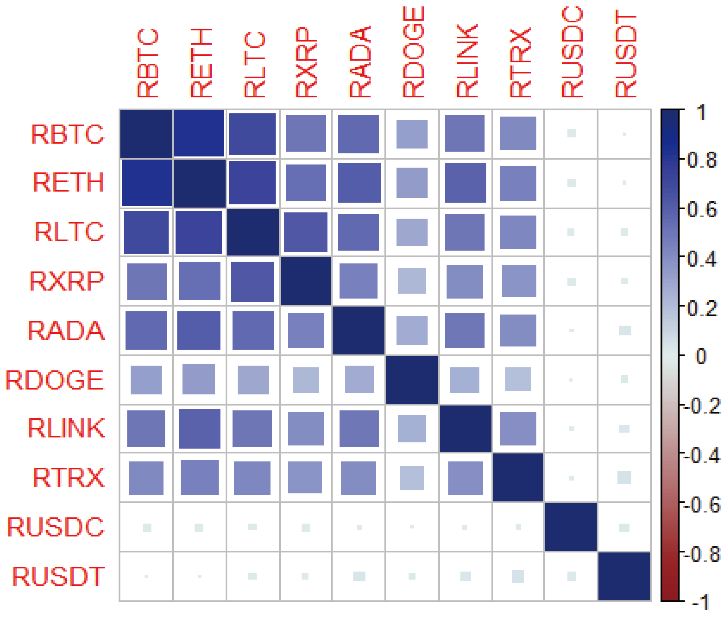
Figure 2.
Bar charts representing distribution of weights during holding and rebalancing periods using the Sharpes minimization strategy. Source- Elaborated by the author.
Figure 2.
Bar charts representing distribution of weights during holding and rebalancing periods using the Sharpes minimization strategy. Source- Elaborated by the author.
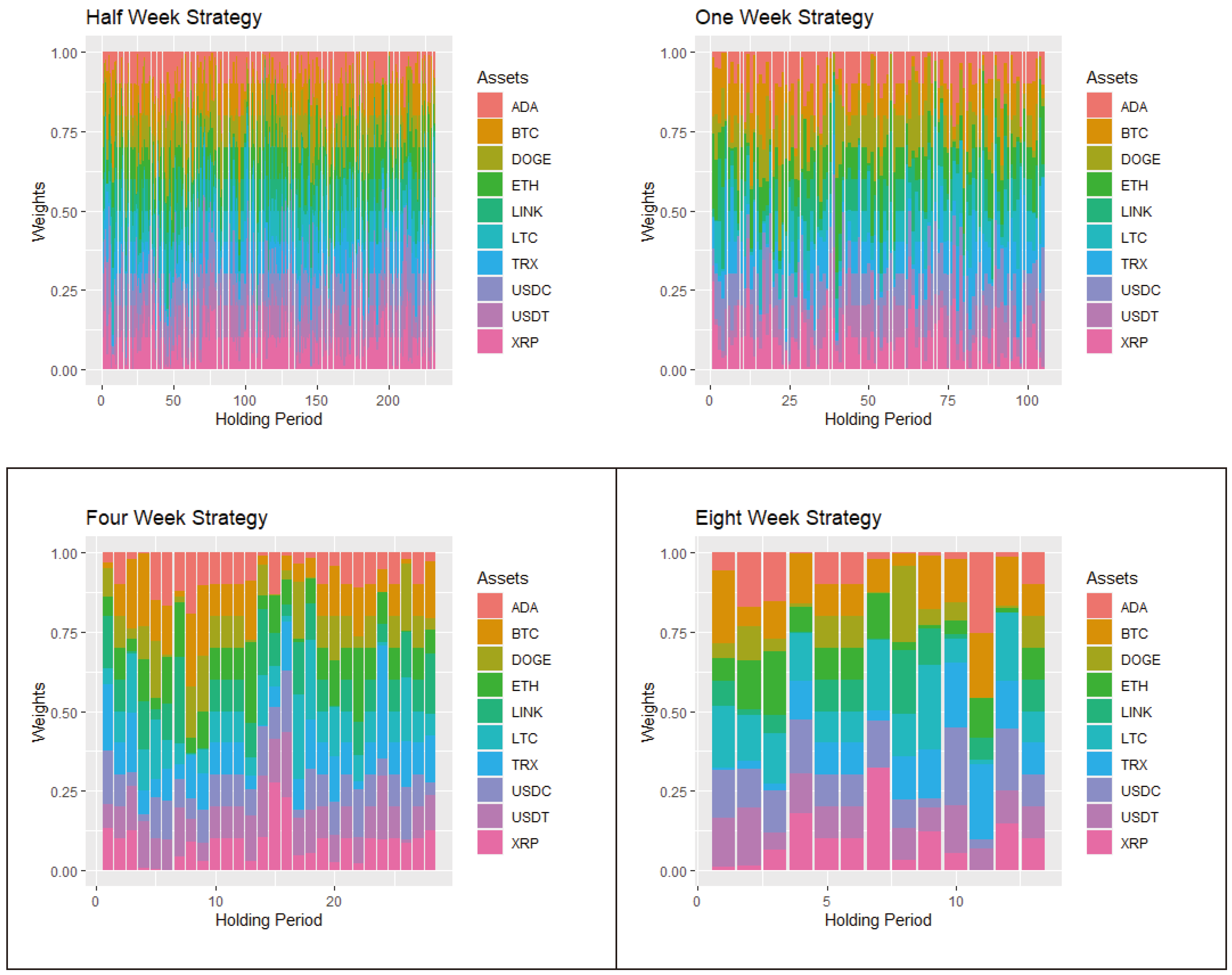
Figure 3.
Bar charts representing distribution of weights during holding and rebalancing periods using the kurtosis minimization strategy. Source- Elaborated by the author.
Figure 3.
Bar charts representing distribution of weights during holding and rebalancing periods using the kurtosis minimization strategy. Source- Elaborated by the author.
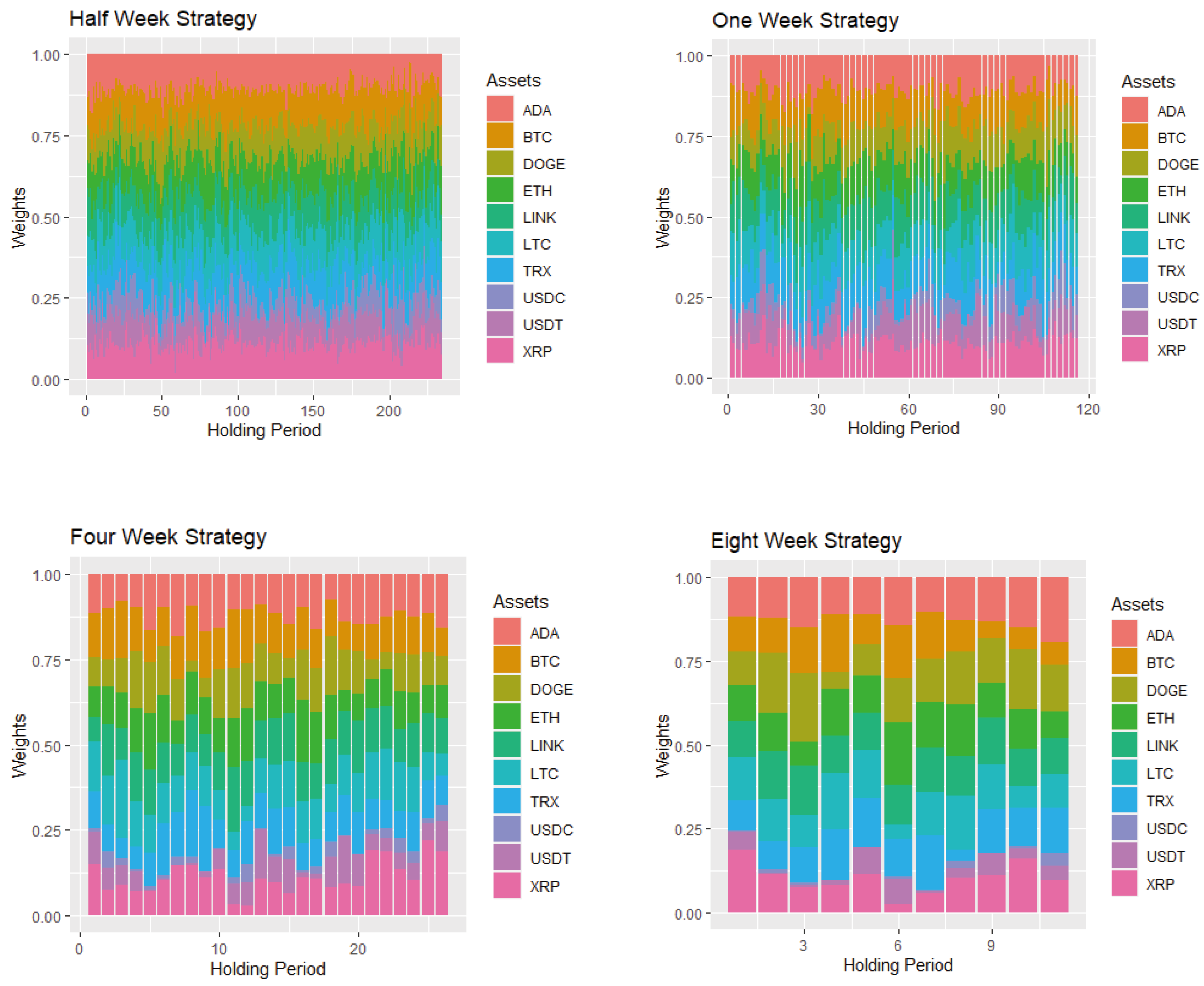
Figure 4.
Comparison of Portfolio Returns Behavior under Different Methodologies and Strategies. Source- Elaborated by the author.
Figure 4.
Comparison of Portfolio Returns Behavior under Different Methodologies and Strategies. Source- Elaborated by the author.
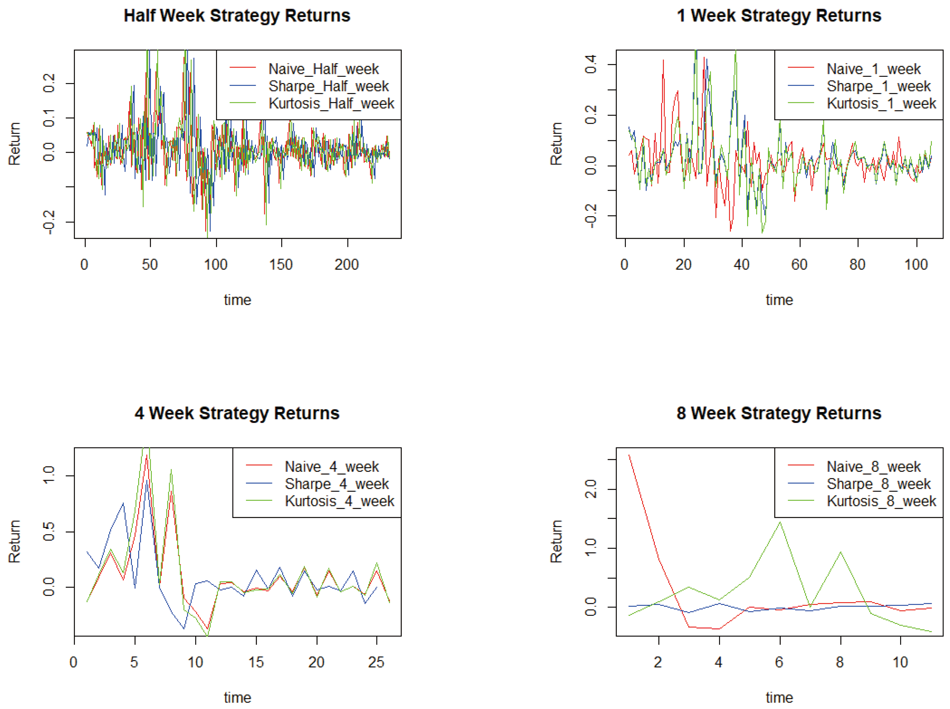

Table 1.
shows the descriptive statistics of daily returns of the 10 cryptocurrencies.
| Descriptive statistics | Bitcoin | Cardano | Chainlink | Dogecoin | Ethereum | Litecoin | Ripple | Tron | Tether | USD coin |
|---|---|---|---|---|---|---|---|---|---|---|
| Minimum | -8.00% | -25.31% | -36.04% | -31.73% | -14.77% | -45.17% | -54.32% | -18.97% | -3.99% | -30.34% |
| Maximum | 11.84% | 29.44% | 20.52% | 37.84% | 7.37% | 13.29% | 24.44% | 26.68% | 5.84% | 30.74% |
| Range | 19.84% | 54.75% | 56.56% | 69.57% | 22.14% | 58.46% | 78.76% | 45.65% | 9.83% | 61.08% |
| Mean | 0.01% | 0.01% | 0.00% | 0.02% | 0.01% | 0.00% | 0.01% | 0.01% | 0.00% | 0.00% |
| Median | 0.01% | 0.00% | 0.00% | 0.00% | 0.01% | 0.01% | 0.02% | 0.00% | 0.00% | 0.00% |
| Satndard Deviation | 0.71% | 1.27% | 1.40% | 1.94% | 0.92% | 1.14% | 1.37% | 1.19% | 0.19% | 0.45% |
| Coefficient of Variation | 114.18 | 159.26 | 607.00 | 116.96 | 114.76 | 654.10 | 257.33 | 186.45 | 23808.26 | -22843.35 |
| Skewness | -0.17 | -3.09 | -1.34 | 0.87 | -0.65 | -4.54 | -3.09 | -0.04 | 0.67 | 0.41 |
| Kurtosis | 21.30 | 36.47 | 48.47 | 56.89 | 18.29 | 167.47 | 166.85 | 39.43 | 173.69 | 2185.35 |
| Jarque Bera Test (p-value) | 0.00 | 0.00 | 0.00 | 0.00 | 0.00 | 0.00 | 0.00 | 0.00 | 0.00 | 0.00 |
1 Source: Elaborated by the author.
Table 2.
presents the returns holding period from 2020 to 2023.
| Rebalancing Frequency | Naive Portfolio | Sharpe-maximization methodology | Kurtosis-minimization methodology |
|---|---|---|---|
| Half-week | 426.82% | 384.55% | 491.45% |
| One-week | 429.18% | 859.18% | 531.03% |
| Four-week | 345.30% | 187.16% | 379.40% |
| Eight-week | 301.01% | 332.03% | 335.79% |
Source- Elaborated by the author.
Table 3.
presents the returns holding period for one year.
| Rebalancing Frequency | Naive portfolio | Sharpe-maximization methodology | Kurtosis-minimization methodology |
|---|---|---|---|
| Half-week | 83.89% | 99.80% | 116.43% |
| One-week | 107.67% | 169.57% | 124.34% |
| Four-week | 92.53% | 58.83% | 98.87% |
| Eight-week | 83.89% | 86.96% | 90.72% |
Source- Elaborated by the author.
Disclaimer/Publisher’s Note: The statements, opinions and data contained in all publications are solely those of the individual author(s) and contributor(s) and not of MDPI and/or the editor(s). MDPI and/or the editor(s) disclaim responsibility for any injury to people or property resulting from any ideas, methods, instructions or products referred to in the content. |
© 2024 by the authors. Licensee MDPI, Basel, Switzerland. This article is an open access article distributed under the terms and conditions of the Creative Commons Attribution (CC BY) license (http://creativecommons.org/licenses/by/4.0/).
Copyright: This open access article is published under a Creative Commons CC BY 4.0 license, which permit the free download, distribution, and reuse, provided that the author and preprint are cited in any reuse.


