
Submitted:
18 February 2024
Posted:
20 February 2024
You are already at the latest version
Abstract
This paper provides the first-time ever analytic modelling for Pointwise Stationary Fluid Flow Approximation(PSFFA) model of the non-stationary
Keywords:
Time Varying queue
; modelling
; simulation
; Pointwise Fluid Flow Approximation (PSFFA)
1. Introduction
The field of transient/non-stationary analysis has limited literature, which can be categorized into simulation, transient analysis, analysis, and applications techniques. These categories encompass various approaches to studying systems that change over time, including simulations, analysing transient behaviour, and exploring non-stationary phenomena. In certain cases, mathematical transformations can be used to obtain a closed form expression for analysing non-stationary queueing systems. However, evaluating these expressions can be computationally complex. As a result, there has been a focus on numerically determining the transient behaviour of such systems instead of deriving closed form expressions.
The current exposition contributes to solving for first time ever, the longstanding unsolved problem of obtaining the state variable of the time varying queueing system.
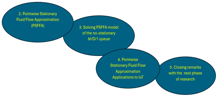
The following flowchart shows how this paper is organized.
2. PSFFA
Let and serve as the temporal flow in, and fow outrespectively. Therefore,
links server utilization, and the time-dependent mean service rate, by:
For an infite queue waiting space:
Thus (2.1) rewrites to:
The stable subcase of (2.4) (i.e., 0), implies:
The numerical invertibility of , yields
Hence,
The queueing system is made of Poisson arrival, one exponential (Poisson) server, FIFO (First-In-First-Out). Thus, queueing system’s - (c.f., [1]) reads:
Therefore, the time varying queueing system’s -PSFFA model reads:
Non-staionary queues’ life example [6] is depicted by Figure 1.
3. Solving the non-stationary queueing system’s PSFFA (c,f., (2.9))
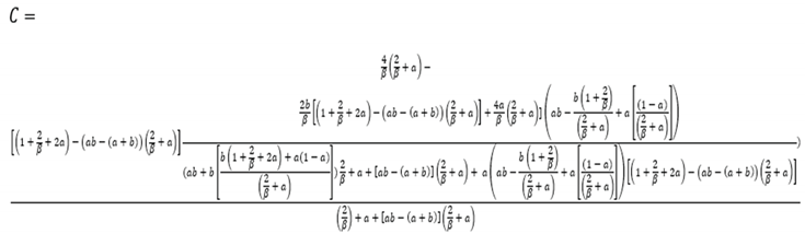
Theorem 3.1 Ismail’s ration, solves (2.9), with a closed form expression to read as:
Proof
We have
Let, then . Setting, Thus, we have
Therefore, we have
where
Let
Hence, it is implied that:
Therefore, we have
 This finally solves the complicated mathematical computations to obtain:
Integrating both sides, implies
This transforms to the final required closed form solution:
By mathematical analysis, it is well known that:
with the domain of real line with zero removed
This finally solves the complicated mathematical computations to obtain:
Integrating both sides, implies
This transforms to the final required closed form solution:
By mathematical analysis, it is well known that:
with the domain of real line with zero removed
Thus, one gets
Corollary 2:
As , we have
Implying
Corollary 3
As , we have
Numerical experiments
Numerical experiment One
Let then , We have
Figure 2 shows a new phenomenon to queuing theorist. The possibility that time will converge to a certain value for sufficiently large number in the time varying queuing system. This is for an increasing temporal mean service rate.
This shows that as the time varying queuing system’s state variable becomes sufficiently large, time vanishes.
Numerical experiment Two
Let then
We have
Figure 3 visualizes a new phenomenon to queuing theorist. The possibility that time will converge to a certain value for sufficiently large number in the time varying queuing system. This is for a decreasing temporal mean service rate.
4. Some PSFFA applications to IoT
By describing how vehicles in a platoon use 802.11p communication to exchange messages and change their movement characteristics at intersections, a time-dependent model for assessing the platooning communications’ effectiveness at intersections phase was thoroughly investigated[7]. The model evaluates the effectiveness of platooning communications and addresses potential safety concerns by considering variables including vehicle behaviours, traffic signals, and the changing connectivity among vehicles.
The authors [7] used PSFFA to describe the transmission queue’s dynamic behaviour in platooning communications. They also create models that characterise the continuous backoff freeze and four access categories (ACs) of 802.11p as they relate to the time-dependent access procedure.
For 802.11p communication in platooning situations at junctions, the authors created models. [7] consider continual backoff freezing and use the PSFFA to describe the gearbox queue’s dynamic behaviour. The access process with its four Access Categories (ACs), they also use a z-domain linear model was demonstrated by [7].
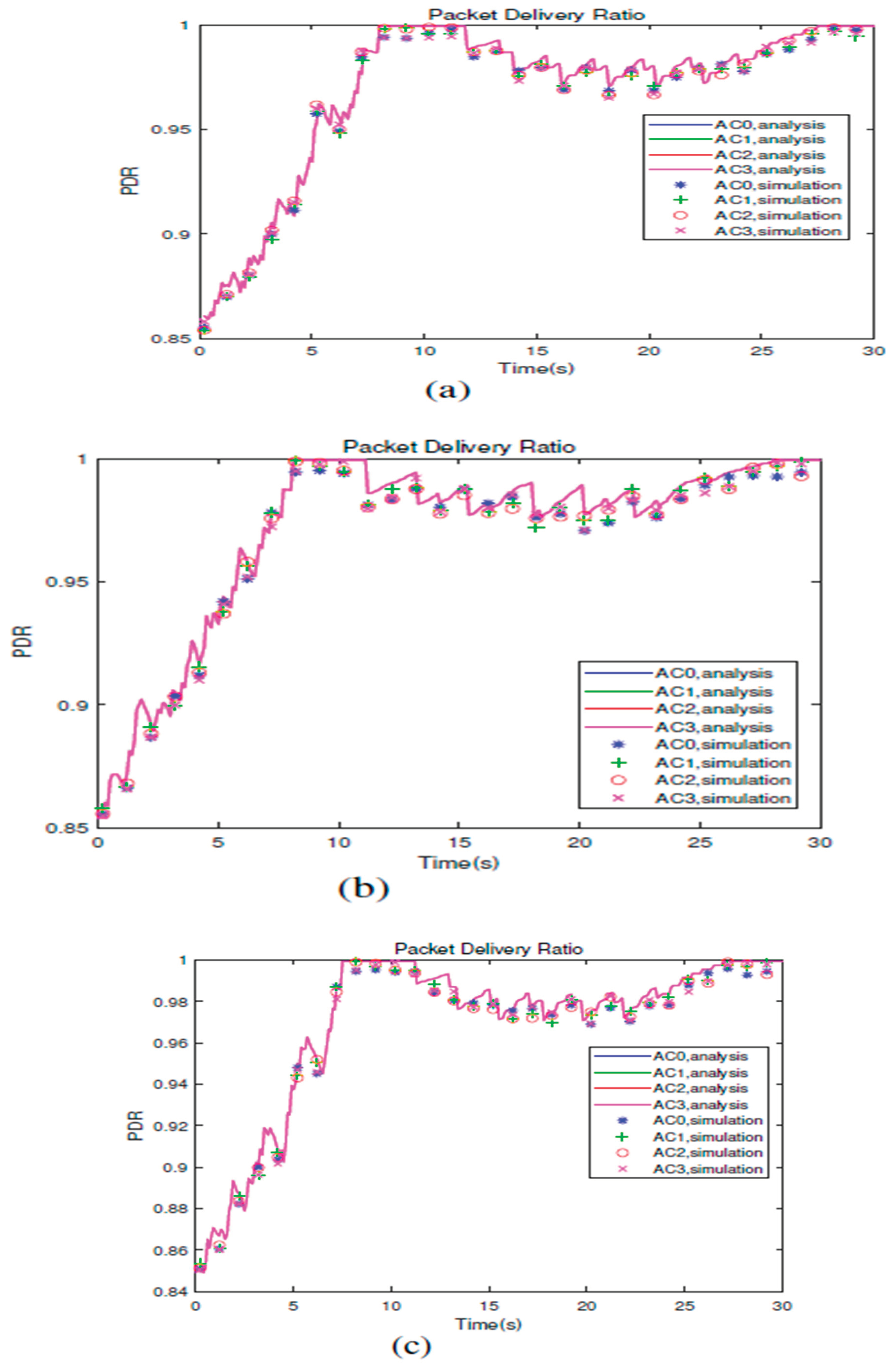
The display of time-dependent packet transmission delay and packet delivery ratio of four Acs can be visualized by Figure 4a, Figure 4b, Figure 4c, Figure 5a, Figure 5b and Figure 5c, respectively.
The findings of a study[8] into the variables influencing queue utilisation dynamics on routers in telecommunication networks. The investigation shows that the average queue length reaches a steady state value following a transient process lasting from a few to tens of seconds when utilising a dynamic model, specifically PSFFA. It is advised to calculate the average queue length using steady state estimations only after the transient process has finished and a more precise differential model may be used.
To accurately predict the average queue length while analysing the average queue length and Quality of Service[8] in a network, a dynamic model with a nonlinear differential equation must be used. Only when the transient process has ended, and the length of the transient process is controlled by variables like flow rate, router interface capacity, and service discipline, are steady-state estimations useful for determining the average queue length. A better choice of queuing models and smaller packet sizes can further hasten the average queue length's convergence.
5. Closing remarks with next phase of research
In this work, a challenging topic in queueing theory is examined; more precisely, the underlying queue’s state variable is determined. The article offers a solution to this issue by utilizing a pointwise stationary fluid flow approximation (PSFFA) technique to formulate the non-stationary queueing system. Future work will concentrate on resolving open research issues and investigating applications of non-stationary queues in other scientific areas. The study also examines the effects of time, combined with and queueing parameters on the underlying queue’s stability dynamics. More fundamentally, some interesting PSFFA applications to IoT are provided. Future work involves further investigation of the impact of on the stability of PSFFA model of t queueing systems.
References
- Zhao, x.; et al. A Queuing Network Model of a Multi-Airport System Based on Point-Wise Stationary Approximation. Aerospace 2022, 9. [Google Scholar] [CrossRef]
- Dr Ismail A Mageed. Solving the Open Problem of Finding the Exact Pointwise Stable Fluid Flow Approximation (PSFFA) State Variable of a Non-Stationary M/M/1 Queue with Potential Real-Life PSFFA Applications to Computer Engineering, 28 January 2024, PREPRINT (Version 1) available at Research Square. [CrossRef]
- Mageed, I.A.; Zhang, Q. Solving the open problem for 𝐺𝐼/𝑀/1 pointwise stationary fluid flow approximation model (PSFFA) of the non-stationary 𝐷/𝑀/1 queueing system. Electron. J. Comput. Sci. Inf. Technol. 2023, 1, 1–6. [Google Scholar]
- Mageed, D.I.A. Upper and Lower Bounds of the State Variable of 𝑀/𝐺/1 PSFFA Model of the Non-Stationary M/Ek/1 Queueing System. Preprints 2024, 2024012243. [Google Scholar] [CrossRef]
- Hu, L.; Zhao, B.; Zhu, J.; Jiang, Y. Two time-varying and state-dependent fluid queuing models for traffic circulation systems. Eur. J. Oper. Res. 2019, 275, 997–1019. [Google Scholar] [CrossRef]
- Mageed, D.I.A. Ismail’s Ratio Conquers New Horizons the Non-stationary M/G/1 Queue’s State Variable Closed Form Expression. Preprints 2024, 2024020548. [Google Scholar] [CrossRef]
- Wu, Q.; Zhao, Y.; Fan, Q. Time-dependent performance modeling for platooning communications at intersection. IEEE Internet Things J. 2022, 9, 18500–13. [Google Scholar] [CrossRef]
- Yeremenko, O.; Lebedenko, T.; Vavenko, T.; Semenyaka, M. Investigation of queue utilization on network routers by the use of dynamic models. In 2015 Second International Scientific-Practical Conference Problems of Info communications Science and Technology (PIC S&T.
Figure 1.
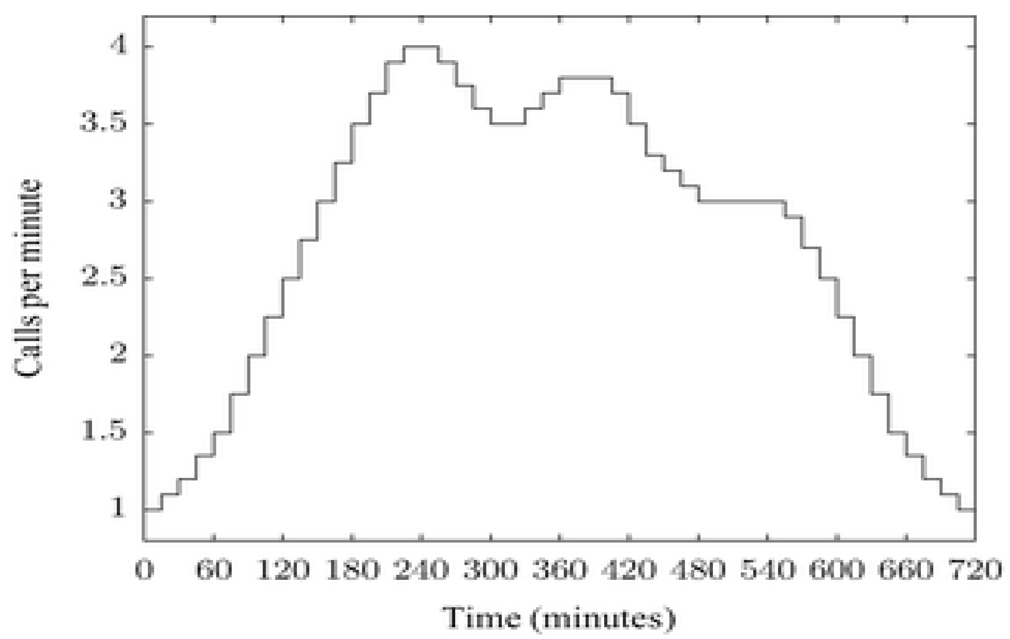
Figure 2.
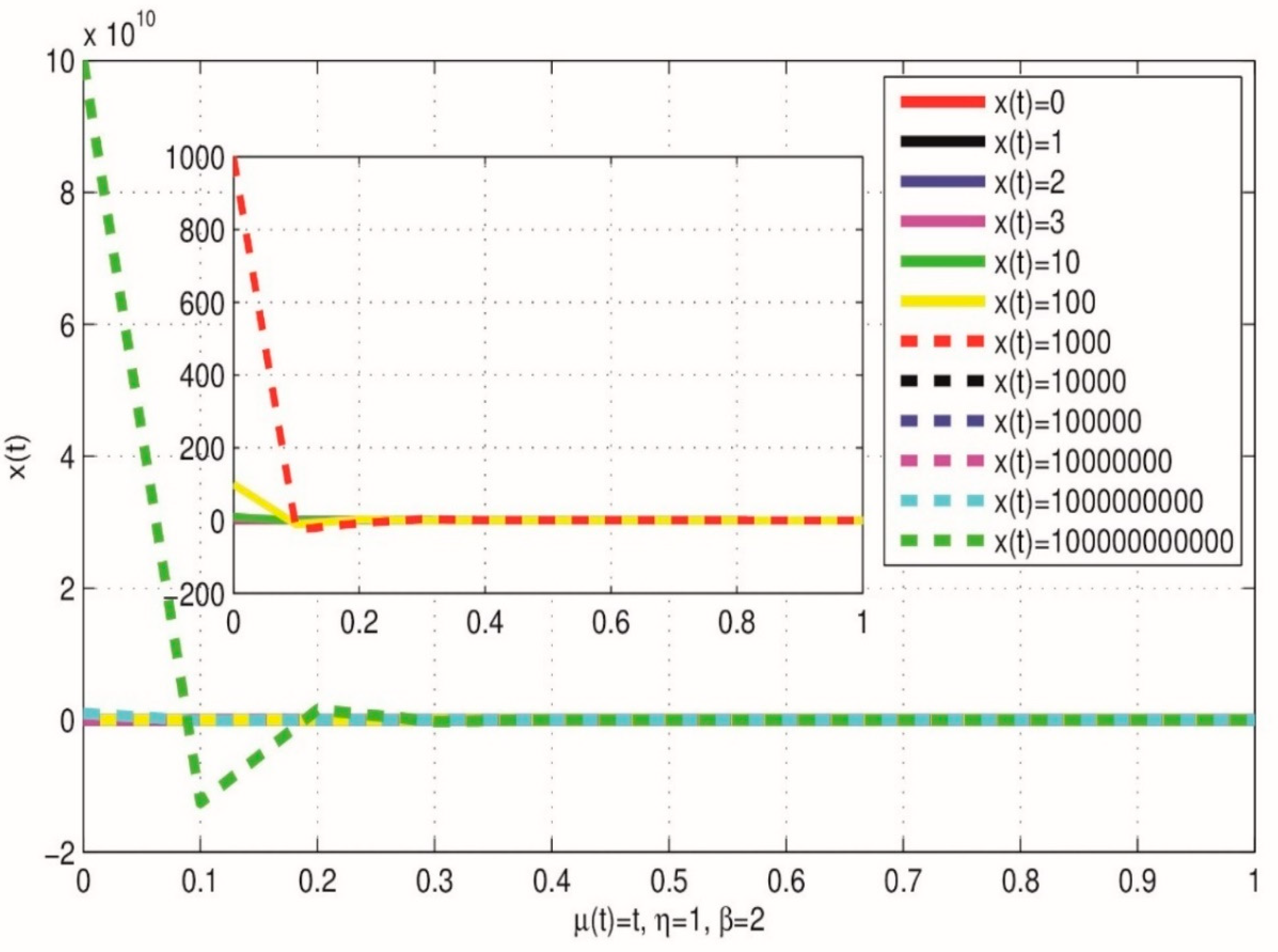
Figure 3.
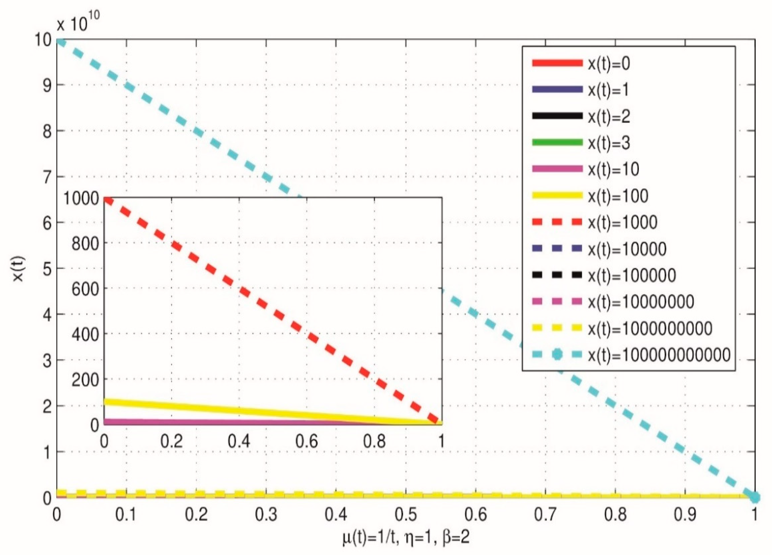
Figure 4.
The packet transmission delay that is time dependent. A left turn, a straight shot, or a right turn, respectively[7].
Figure 4.
The packet transmission delay that is time dependent. A left turn, a straight shot, or a right turn, respectively[7].
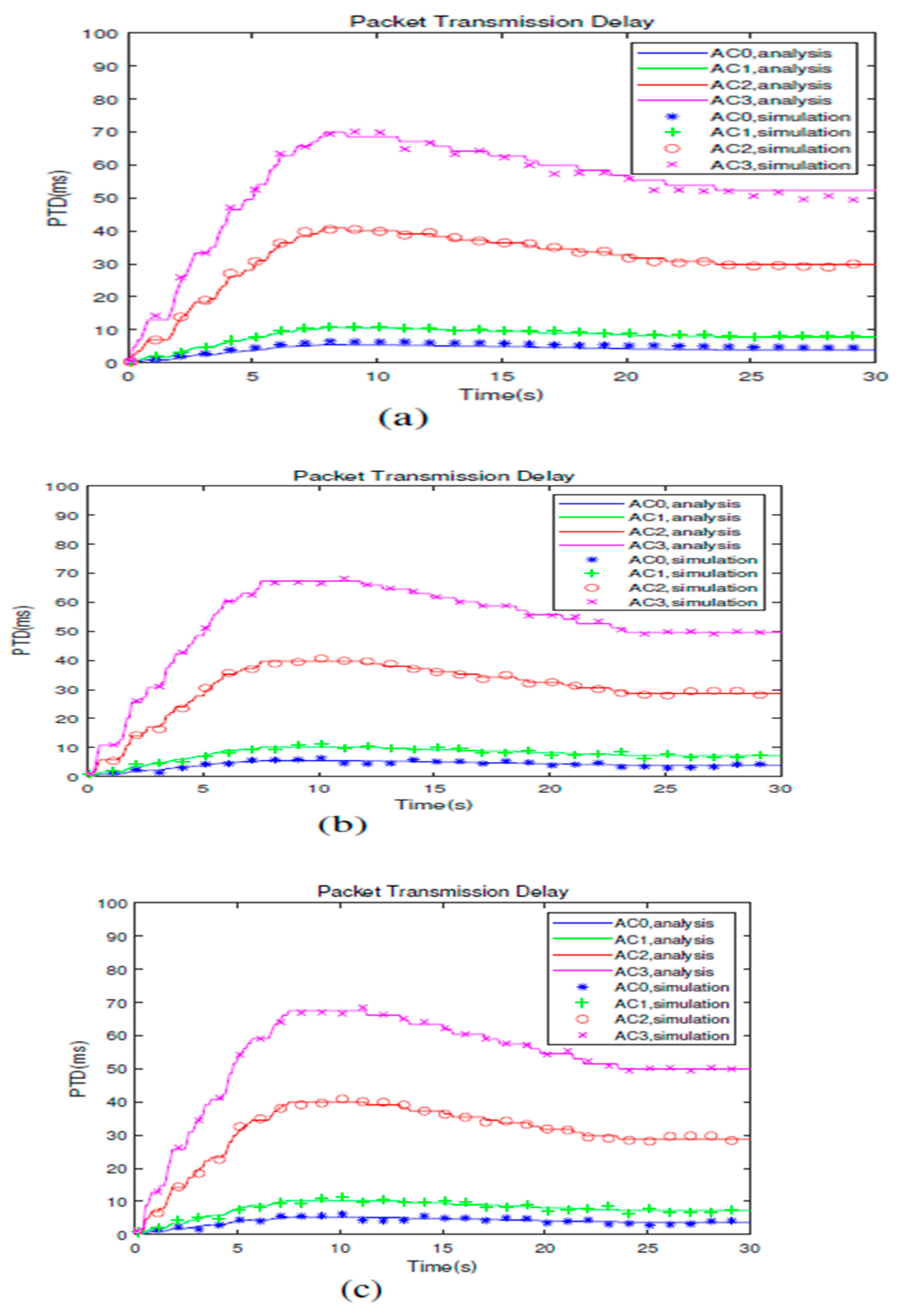
Figure 5.
The proportion of time-dependent packet deliveries. A left turn, a straight shot, or a right turn, respectively[7].
Figure 5.
The proportion of time-dependent packet deliveries. A left turn, a straight shot, or a right turn, respectively[7].
Disclaimer/Publisher’s Note: The statements, opinions and data contained in all publications are solely those of the individual author(s) and contributor(s) and not of MDPI and/or the editor(s). MDPI and/or the editor(s) disclaim responsibility for any injury to people or property resulting from any ideas, methods, instructions or products referred to in the content. |
© 2024 by the authors. Licensee MDPI, Basel, Switzerland. This article is an open access article distributed under the terms and conditions of the Creative Commons Attribution (CC BY) license (http://creativecommons.org/licenses/by/4.0/).
Copyright: This open access article is published under a Creative Commons CC BY 4.0 license, which permit the free download, distribution, and reuse, provided that the author and preprint are cited in any reuse.


