
Submitted:
12 February 2024
Posted:
13 February 2024
You are already at the latest version
Abstract
Speech recognition, also known as automatic speech recognition (ASR), is a technology that enables software to transcribe spoken language into text. However, existing Amharic ASR methods require multiple separate blocks, such as language, acoustic, and pronunciation models with dictionaries, which can be time-consuming and influence performance. This study proposes an approach that replaces much of the speech pipeline with a single recurrent neural network (RNN) architecture. Our proposed architecture is based on a hybrid approach that combines a convolutional neural network (CNN) with a recurrent neural network (RNN) and a connectionist temporal classification (CTC) loss function. We conducted several experiments with noisy audio data that contain 20,000 valid sentences. The model was evaluated using the word error rate (WER) metric, achieving impressive results of 7% WER on noisy data. This approach has significant implications for the field of speech recognition, as it reduces the human effort required to create dictionaries and improves the efficiency and accuracy of ASR systems, making them more practical for real-world applications.
Keywords:
Automatic speech recognition
; Convolutional Neural Network
; Connectionist Temporal Classification
; End-to-End
; Neural network
; Noisy
; Recurrent Neural Network
; Subspace filtering
; Spectral Subtraction
1. Introduction
Speech recognition, commonly referred to as automatic speech recognition (ASR), computer speech recognition, or speech-to-text, is a feature that allows software to convert spoken language into written text. Despite being sometimes confused with voice recognition, speech recognition focuses on converting speech from a verbal to a text format, whereas voice recognition only aims to distinguish the voice of a certain person.
Different speech technology applications are being used by a wide range of industries nowadays, which is assisting both businesses and consumers in saving time and even lives (Hanan Aldarmaki, Asad Ullah, and Nazar Zaki, 2021).
There are various methods used to create automatic speech recognition. These methods include Data Time Wrapping (DTW), Hidden Markov Model (HMM), Dynamic Bayesian Network (DBN), and artificial neural network (ANN) (Hebash H.O. Nasereddin, January 2018). HMM and NN is the most commonly used method in recent times for speech recognition. HMM works by breaking down speech signals into a sequence of states and then using the acoustic properties of the speech to determine the likelihood of a sequence of phones (Kebebew, 2010).
Although neural networks (Bourlard & Morgan, 1993; Hinton et al., 2012) have significantly assisted automatic speech recognition, they now make up only one portion of a complicated pipeline. Like in conventional computer vision, the pipeline’s first step is the extraction of input features. Common methods include vocal tract length normalization and Mel-scale filterbanks (Davis & Mermelstein, 1980) (with or without a further transform into Cepstral coefficients) (Lee & Rose, 1998). Then, emission probabilities for a hidden Markov model are reconstituted from the neural network output distributions. The neural networks are then trained to recognize specific audio input frames (HMM).
Consequently, the actual performance metric and the goal function used to train the networks are very different (sequence-level transcription accuracy). This is the kind of consistency that end-to-end learning is designed to avoid. The fact that a considerable improvement in frame accuracy can lead to a little improvement or even a deterioration in transcription accuracy puzzles researchers. Another problem is that the frame-level training targets must be inferred from the alignments the HMM obtained. As a result, in an uncomfortable iterative process, network retraining and HMM re-alignments are alternated to provide targets that are more exact. Direct training of HMM neural network hybrids has been done using full-sequence training techniques like Maximum Mutual Information to increase the likelihood of accurate transcription (Bahl et al., 1986; Jaitly et al., 2012). However, these methods can only be used to retrain a system that has already been trained at the frame level, and they necessitate the careful adjustment of several hyperparameters, often much more than for deep neural networks.
The goals that are provided to the networks are often phonetic, despite the fact that the transcriptions used to train speech recognition systems are lexical. In order to translate words into phoneme sequences, a pronunciation dictionary is required. Such dictionaries need a lot of human effort to create, and they frequently have a big impact on performance (Graves, A., & Jaitly, N., 2014). Another source of expert information, "state tying," is required to lessen the number of target classes since co-articulation effects are taken into account by multi-phone contextual models, which adds another layer of complexity.
The model proposed in this research aims at replacing as much of the speech pipeline with single recurrent neural network (RNN) architecture. While it is possible to directly transcribe unprocessed speech waveforms using RNNs (Graves, 2012, Chapter 9) or features learnt using limited Boltzmann machines (Jaitly & Hinton, 2011), the computational cost is significant and the performance typically lags behind conventional preparation. As a result, we have settled on spectrograms as the bare minimum preprocessing method.
This research aims to address important issues in addition to solving scientific issues. The difficulties that hearing-impaired people have in understanding other people’s speeches makes it difficult for them to interact with nonhearing-impaired people, which prevents them from learning about their surroundings. Our work fasters typing directly from human voice, which is great for people who struggle with precise word placement. Therefore, we came up with the notion of creating an end-to-end speech recognition model that transforms speech into text in order to get around those difficulties and make life easier.
To the best of our knowledge, previous speech recognition models for Amharic language are built using traditional speech recognition mechanisms using acoustic, pronunciation, language models with a relatively smaller number of clean data, without considering noisy data and automatic feature extraction. currently available end-to-end pipelines do not take into account the presence of noisy data, and their feature extraction methods do not utilize neural networks (Baye, A., Tachbelie, Y., & Besacier, L. ,2021). However, we propose an end-to-end speech recognition mechanism which enables us to directly convert speech to text by replacing those traditional pipelines with a single RNN pipeline. So, unlike traditional HMM based speech recognition models, our speech recognition model will not have those individual pipelines, for example, pronunciation dictionaries are not needed in our case. So, our study saves the time spent for preparing those dictionaries and finding domain expertise in certain areas.
End-to-end is a system which directly maps a sequence of input acoustic features into a sequence of grapheme or words. We are expecting that our end-to-end speech recognition model will greatly simplifies the complexity of traditional speech recognition. With the advancements in neural networks, the need for manual labeling of language and pronunciation information is significantly reduced, as the neural network can now autonomously learn and capture such information. According to the literature, there are two main structures for end-to-end speech recognition (Baye, A., Tachbelie, Y., & Besacier, L. ,2021); attention model and CTC. We have used CTC in our case and it has solved the alignment problem occurred in traditional models.
This study attempts to answer the following research questions:
- Is applying erosion to the spectrograms has significant effect to speech recognition model?
- Which noisy reduction mechanism is better from spectral subtraction, subspace filtering and both in combined?
- Which deep learning algorithm (from LSTM, BILSTM, GRU and BiGRU) performs better to build an end-to-end speech recognition model for Amharic?
2. Methods and Materials
2.1. Data Collection and Processing
Collecting Audios and Recording Speeches:we conducted audio recordings of individuals delivering speeches in the Sidama region, where Amharic is not their primary language. The noisy dataset consists of 400 distinct sentences, each sentence being read by 50 different individuals. In total, 20,000 sentences are used for the recordings. The noisy audios are read speech data which last from a minimum of 4 seconds to a maximum of 20 seconds. The total noisy data is around 44 hours and 46 minutes.
Transcriptions:For the speech recording (noisy data), a corresponding transcription was created. This process involved carefully listening to the audio and converting it into written text. The text data serves as the ground truth for the deep learning model, allowing it to learn the relationship between the audio features and the corresponding text.
The transcribed text paired with the file name of the audio is presented in Figure 1 below.
The collected data is analyzed to gain insight into speech characteristics and develop effective methods for noise reduction. The data is and converted to spectrograms using Short-Time Fourier Transform (STFT) for feature extraction. The resulting spectrograms are then used as input to the neural network. In general, the research aims to contribute to the development of improved speech recognition and processing technologies.
Training and Validation Phases: The training phase is a critical step in developing a speech recognition system. It involves training a neural network model, specifically a combination of recurrent neural network (RNN) variants and neural network (CNN), to recognize speech patterns and convert them into text. The training data, which consists of a mixture of noisy-free and noisy speech data, is used to adjust the model’s parameters and improve its accuracy. The training process continues until the model achieves satisfactory accuracy on the training data.
Following the training phase, the validation/testing phase is conducted to evaluate the system’s performance on unseen data. A separate validation data set, derived from the training data, is used for this purpose. The goal of the validation phase is to monitor the system’s performance and prevent overfitting, which refers to a situation where the model performs well on the training data but poorly on new, unseen data. The accuracy of the predicted transcription in the validation data is measured using the Word Error Rate (WER) metric. The model’s hyperparameters, such as the learning rate, number of layers, and number of neurons, are adjusted during the validation phase to improve accuracy on the validation data.
2.2. Model Architecture
The architecture is a deep learning model designed for automatic speech recognition (ASR). It is based on a hybrid approach that combines a convolutional neural network (CNN) with a recurrent neural network (RNN) and a connectionist temporal classification (CTC) loss function.
Here is an overview of the model architecture with BiGRU layers:
Input: The input is a spectrogram representation of the audio data.
Convolutional Layers: A series of 2D convolutional layers with batch normalization and ReLU activation are applied to the input to extract relevant features.
Bidirectional GRU Layers: After the convolutional layers, a few layers of BiGRU are applied. These layers consist of two parallel GRUs for each layer: one that processes the sequence in the forward direction and another in the backward direction. The outputs of both GRUs are combined to capture information from both directions.
Fully Connected Layer: The output of the final BiGRU layer is passed through a fully connected layer with a linear activation function.
CTC Loss: Connectionist Temporal Classification (CTC) loss is used during training to align the predictions with the target labels without requiring a pre-segmentation of the input data. The architecture is presented in Figure 2 below.
2.3. Model Implementation
This study describes the implementation of a model, an end-to-end automatic speech recognition (ASR) system. The implementation is based on a TensorFlow/Keras model, using convolutional layers, bidirectional recurrent layers, and dense layers to process the input spectrograms and produce character probabilities.
Input and Pre-processing
The model’s input is defined as a variable-length sequence of spectrograms, where each spectrogram has input_dimfrequency bins. The ‘None’in the shape of the input indicates that the sequence length can vary. The input spectrograms are reshaped to have an extra dimension, which is required for the convolutional layers. This extra dimension is a singleton dimension, represented by 1. The input layer takes a 3D tensor as input, with the first dimension being the batch size, the second dimension being the time steps (which is set to None to accept variable length sequences), and the third dimension being the input feature dimension (input_dim). The name of the input layer is set to "input". And then reshapes the input tensor to have an additional dimension of size 1, which is required for the 2D convolutional layer. The second dimension is set to -1 to automatically infer the number of time steps. The input to the model is a spectrogram with shape ‘(None, input_dim)‘, where ‘None‘ represents the variable-length time dimension. The input is first reshaped to include an additional channel dimension, resulting in a shape of ‘(-1, input_dim, 1)‘. This step is necessary to apply 2D convolutional layers to the input spectrogram.
Convolutional Layers
The customized CNN architecture used by the model includes two convolutional layers that serve the purpose of extracting useful features from the input audio spectrogram. The input audio spectrogram is a 2D representation of the audio signal, where the time domain is mapped to the horizontal axis, and the frequency domain is mapped to the vertical axis.
The first convolutional layer applies a set of learnable filters to the input spectrogram, producing a set of output feature maps that capture local patterns and structures within the spectrogram. The second convolutional layer then applies another set of filters to these output feature maps, further extracting higher-level features that are more relevant to the task at hand.
By applying these convolutional layers, the model is able to automatically learn relevant features from the input spectrogram without the need for manual feature engineering. This is a key advantage of using a CNN architecture for audio processing, as it allows the model to adapt to a wide range of input data and capture important patterns that may not be immediately apparent to a human expert.
As mentioned above the architecture of the customized CNN model used for speech recognition includes two convolutional layers that play a crucial role in the feature extraction process. The first convolutional layer applies a 2D convolution operation with a kernel size of 11x41 and a stride of 2x2 to the input spectrogram, resulting in the extraction of 32 feature maps. The size of the kernel and stride values are chosen carefully based on the desired properties of the features that need to be extracted. For instance, a larger kernel size can capture more global features, while a smaller kernel size can capture more local features.
Similarly, the second convolutional layer applies another 2D convolution operation with a kernel size of 11x21 and a stride of 1x2 to the output feature maps of the first convolutional layer. This operation also extracts 32 feature maps from the input spectrogram, but with a different filter size and stride, which enables the network to capture additional features that may have been missed by the first convolutional layer.
After the two convolutional layers have been applied, the output is then reshaped into a single dimension to prepare it for input into the recurrent layers of the network. The purpose of these recurrent layers is to model the temporal dependencies between the extracted features and generate a transcription of the input speech signal.
Recurrent layers, unlike traditional feedforward neural networks, are capable of processing sequential data by using the output of the previous time-step as input to the current time- step. In the context of speech recognition, this means that the recurrent layers are able to model the temporal dependencies between the extracted features, which can be useful for identifying important speech features that may occur over a longer period of time.
Overall, the combination of convolutional and recurrent layers in the customized CNN architecture allows the model to effectively extract features from the input spectrogram and model the temporal dependencies between them to generate accurate transcriptions of speech signals.
The use of batch normalization and ReLU activation functions after the convolutional layers is a common practice in deep learning to improve the performance of neural networks. Batch normalization normalizes the output of each batch, which helps to reduce internal covariate shift, resulting in more stable and faster training. Additionally, ReLU activation introduces non-linearity to the output of each convolutional layer, allowing the network to learn more complex and nonlinear features from the input spectrogram.
The first convolutional layer with 32 filters, a kernel size of (11, 41), and a stride of (2, 2) is designed to extract broad local features from the input spectrogram. The use of padding ensures that the output of the layer has the same spatial dimensions as the input, which is important for subsequent layers.
The second convolutional layer with 32 filters, a kernel size of (11, 21), and a stride of (1, 2) captures more fine-grained local features of the input spectrogram. Like the first layer, the use of padding ensures that the output of the layer has the same spatial dimensions as the input.
Overall, the combination of convolutional layers, batch normalization, and ReLU activation functions in the CNN architecture helps the model to learn useful local features from the input spectrogram, which are then used by the recurrent layers to generate transcriptions of the input speech signal.
Reshaping for RNN Layers
In order to prepare the output of the second convolutional layer to be used by the recurrent layers, it is necessary to reshape it. This is done by collapsing the height and width dimensions into a single dimension. To calculate this new dimension, we simply multiply the height of the output feature map (which can be accessed using x.shape[-2]) by its width (which can be accessed using x.shape[-1]). By doing this, we create a new, flattened representation of the output feature map that can be more easily processed by the recurrent layers. This is an important step in the overall architecture of the system, as it helps to ensure that the output of the convolutional layers is properly prepared for the subsequent processing that will take place in the recurrent layers.
Recurrent Layers
The RNN layers consist of bidirectional Gated Recurrent Units (GRUs) with tanh activation functions and sigmoid recurrent activations. The number of units in each GRU is specified by the rnn_unitsargument.
The output from the forward and backward GRU layers is concatenated along the last dimension. Dropout is applied after each bidirectional layer, except for the last one.
The model uses a series of bidirectional GRU layers to capture long-range dependencies in the input spectrogram. The number of GRU layers is determined by the ‘rnn_layers‘ parameter. Each GRU layer has ‘rnn_units‘ recurrent units and uses a ‘tanh‘ activation function for the update gate and a ‘sigmoid‘ activation function for the reset gate. The layers return sequences and have a reset-after configuration.
The GRU layers are wrapped with a bidirectional layer with a ‘concat‘ merge mode. A dropout rate of 0.5 is implemented after every bidirectional layer, except for the final layer.
The GRU layer is bidirectional, meaning it processes the input sequence in both forward and backward directions. The output of the GRU layer is concatenated with its inverse, and the resulting tensor is passed to the next layer. If the current iteration is not the last one, a dropout layer with a rate of 0.5 is applied to the output tensor.
In this model, the BiGRU (Bidirectional Gated Recurrent Unit) layer is used to capture both the past and future context of the input spectrogram sequence. The BiGRU layer is a type of recurrent neural network layer that processes the input sequence in both forward and backward directions. The outputs of the forward and backward GRU layers are concatenated and passed to the next layer. This allows the model to capture both the local and global context of the input sequence.
The BiGRU layer in this model has rnn_layers=5, which means that there are 5 BiGRU layers stacked on top of each other. Each BiGRU layer has rnn_units=512GRU units to model the temporal dependencies in the input spectrogram sequence.
The merge_modeparameter of the Bidirectionallayer is set to "concat", which means that the outputs of the forward and backward GRU layers are concatenated before being passed to the next layer.
In this model, the BiGRU (Bidirectional GRU) layers are used for modeling the temporal dependencies in the input spectrogram sequence.
The GRU is a type of recurrent neural network (RNN) layer that is designed to solve the vanishing gradient problem that occurs in traditional RNNs. The GRU has two gates, a reset gate and an update gate, that control the flow of information through the layer. The reset gate determines which information from the previous time step to forget, while the update gate determines which information from the current time step to keep. The GRU computes a new hidden state based on the input and the previous hidden state, which is then passed to the next time step.
In this model, the BiGRU layer is used to encode the input spectrogram sequence into a high-level representation that captures the temporal dependencies in the sequence. By using a bidirectional layer, the model is able to capture both the local and global context of the input sequence. This high-level representation is then fed to a dense layer, which produces the final output sequence.
Dense Layers and Output
There is a dense layer and an output layer following the BiGRU layers. The Dense layer is typically added after the RNN layer to extract high-level features from the sequence data output by the RNN. In this particular model, the Dense layer takes the output of the final BiGRU layer and applies a linear transformation to map it to a higher dimensional space. The number of units in the Dense layer is set twice the number of GRU units in each BiGRU layer, which helps increase the model’s capacity to capture more complex relationships between the input data and the output labels.After the Dense layer, a Rectified Linear Unit (ReLU) activation function is applied to the output to introduce non-linearity to the model. ReLU is a commonly used activation function that sets all negative values in the output to zero while leaving positive values unchanged.
To prevent overfitting, a dropout layer is added to the model after the Dense layer. Dropout randomly sets a fraction of the input units to zero during training, which helps prevent the model from over-relying on specific features and encourages it to learn more robust representations of the input data. In this model, the dropout rate is set to 0.5, meaning that half of the input units are randomly dropped out during training. The output of the dropout layer is then fed into the final softmax activation layer, which generates a probability distribution over the output classes.
The output layer is responsible for producing the final output of the model, which is a sequence of characters representing the transcription of the input speech signal. It is implemented as a Dense layer that maps the output of the previous Dense layer to the final output dimension, which is the number of characters in the vocabulary plus one for the blank character. The softmax activation function is applied to the output of the layer to ensure that the output probabilities sum up to one, making it a probability distribution over the characters in the vocabulary. The blank character is added to the vocabulary to allow the model to output silence or pauses in the speech signal.
Unlike the Dense layer in the model that is followed by the dropout regularization, no dropout regularization is applied to the output layer. This is because dropout regularization randomly drops out some of the output units during training to prevent overfitting, which can degrade the model’s performance when applied to the output layer. Instead, the model relies on the training data and loss function to regularize the output layer and produce accurate transcriptions. The output of the output layer is a sequence of probabilities for each character in the vocabulary, indicating the likelihood of each character being present at a particular time step in the input speech signal. The final transcription is obtained by decoding this probability sequence, which is typically done using the greedy decoding algorithm or beam search decoding algorithm.
The classification layer in a neural network is responsible for performing the final classification of the input data. In the case of this speech recognition model, the classification layer maps the output of the previous layer to the final output dimension, which is the number of characters in the vocabulary plus one for the blank character.
In this connectionist temporal classification (CTC) based speech recognition model, the classification layer is typically a dense layer with output_dim + 1 units and a softmax activation function. The additional unit in the output dimension corresponds to the blank label used in the CTC loss calculation.
The purpose of the blank label is to allow the model to output silence or pauses in the speech signal, and to handle situations where multiple characters occur in the same time step. During training, the CTC loss function automatically handles the alignment between the input audio signal and the corresponding transcription, even if there are variable-length or missing segments. The blank label helps to ensure that the CTC loss function can produce accurate alignments and transcriptions.
2.4. Model Compilation
The compile method is used to configure the model for training by specifying the optimizer and loss function to use during training. In this study, the model is compiled in the following way:
The first step is to define the optimizer to use during training. In this case, the Adam optimizer is used with a learning rate of 1e-4. The Adam optimizer is a popular optimizer that is well-suited for training deep neural networks.
The CTCLossfunction is then used as the loss function for the model. The Connectionist Temporal Classification (CTC) loss function is commonly used in speech recognition tasks (Lee, J., & Watanabe, S., 2021). The CTC loss function is designed to handle variable- length input sequences and output sequences, which is particularly useful for speech recognition where the input is a variable-length audio signal and the output is a variable- length sequence of characters.
Once the optimizer and loss function are defined, the model is compiled. The compilemethod takes two main arguments: the optimizer and the loss function. In this case, the optimizer is set to optand the loss function is set to CTCLoss.
Connectionist Temporal Classification (CTC): The CTC (Connectionist Temporal Classification) layer is a specialized layer used in sequence-to-sequence learning tasks where the input and output sequences have variable lengths, and there is no one-to-one correspondence between the input and output sequence elements. This layer is commonly used in speech recognition tasks, where the input sequence is an audio signal and the output sequence is a sequence of characters.
The CTC layer works by introducing a special "blank" label that can be inserted between any two adjacent labels in the output sequence. This allows the CTC layer to handle variable-length output sequences without requiring an exact alignment between the input and output sequences.
During training, the CTC layer computes the probability of the output sequence given the input sequence, and the CTC loss function is used to measure the difference between the predicted output sequence and the actual output sequence. The goal of training is to minimize the CTC loss function, which encourages the model to learn a mapping from the input sequence to the correct output sequence.
CTC layerfunction is used as the final layer of the model, and is named "ctc_loss".
The labelstensor is the ground truth label sequence, and the outputtensor is the predicted probability sequence. CTCLayerfunction computes the CTC loss function using the predicted probabilities and the ground truth labels, and returns the computed loss as the output of the layer.
The CTC layer is an important component of speech recognition models, as it allows the models to handle variable-length input and output sequences, which is a common challenge in speech recognition tasks. The CTCloss function is defined as follows:
Decoding: The decoding process is the final step in the speech recognition pipeline, and it is responsible for converting the predicted probabilities into the final output sequence. In this model, the decoding process uses the Beam Search algorithm to find the most likely output sequence given the input sequence.
The decode_batch_predictions function first initializes an array of input sequence lengths (input_len) to the length of the input sequence. The function then loops over each sequence in the batch and performs the decoding.
The K.ctc_decode function is used to perform the decoding. The K.ctc_decode function is a built-in function in TensorFlow that can be used to decode the predicted probabilities into a sequence of labels. The greedy parameter is set to False to enable the Beam Search decoding algorithm, and the beam_width parameter is set to the desired beam width. The top_paths parameter is set to 1 to return only the most likely output sequence.
The output of the K.ctc_decode function is a tuple containing the decoded output sequence and the corresponding sequence probability. In this case, only the decoded output sequence is needed, so the [0][0] indexing is used to extract the decoded output sequence.
The decoded output sequence is then converted from numeric labels to characters using the num_to_char function defined earlier. The tf.strings.reduce_join function is used to join the characters into a single string, and the resulting string is converted to a numpy array using the numpy()method. Finally, the decodemethod is used to convert the numpy array to a string in UTF-8 format.
The decoded output sequence is then appended to the resultslist, and the loop continues until all sequences in the batch have been decoded. Finally, the function returns the list of decoded output sequences.
Overall, the decoding process is an important part of the speech recognition pipeline, as it is responsible for converting the predicted probabilities into the final output sequence. The beam search algorithm is a widely used decoding algorithm in speech recognition, as it is able to find the most likely output sequence while taking into account the possibility of alternate paths.
The decode_batch_predictions function is used to perform the decoding for a batch of input sequences. The function takes the predicted probabilities for a batch of input sequences (pred) and the beam size as inputs.
In this CTC decoding, beam search algorithm is used to improve the accuracy of the transcription. Beam search works by maintaining a set of candidate transcriptions and expanding the set at each time step. The algorithm prunes the candidates that are unlikely to be the final transcription based on a score or probability threshold, and continues expanding until a stopping criterion is reached.
2.5. Evaluation Metric
WER is a widely used metric to evaluate speech recognition systems. It measures the percentage of incorrectly recognized words compared to the reference transcription. Substitution, deletion, and insertion errors are considered, and WER is calculated by adding these errors and dividing by the total number of words in the reference. Lower WER indicates better performance and allows for model comparison and hyperparameter tuning.
3. Results
Several experiments have been employed. We have improved the model’s robustness by training it on 44 hours of noisy data. We introduced various noise reduction mechanisms to mitigate the adverse effects of background noise. Specifically, we employed three techniques: spectral subtraction, subspace filtering, and their combination. Spectral subtraction aims to suppress background noise by subtracting an estimated noise spectrum from the noisy speech signal. Subspace filtering uses subspace methods to separate the speech signal from the background noise. We evaluated the model’s performance when trained with each of these noise reduction mechanisms individually and by combining the two techniques. We have calculated Signal to Noise (SNR) ratio which is a metric used to quantify the ratio of the desired signal (such as speech) to the accompanying background noise in an audio signal. It provides the measure of the signal strength relative to the noise level.
We examined the model’s performance when confronted with noisy data. By introducing different noise reduction techniques, we have enhanced the model’s robustness. The WER for noisy data without applying any noise reduction techniques is 10.5%. When we applied spectral subtraction, the WER was reduced to 8.5%, demonstrating a notable improvement in the system’s ability to handle background noise. The subspace filtering technique further enhanced performance, resulting in a reduced WER of 7.4%. The combined technique is effective, with a WER of 7.02% (for detail see Table 1). These results indicate that our model, equipped with advanced noise reduction mechanisms, exhibits strong noise-robustness capabilities. The full results are shown in Table 1.
We have used a frame length of 256 samples and a frame step of 160 samples to extract audio features.
We evaluated the performance of the speech recognition system using the word error rate (WER), calculated as the percentage of words incorrectly recognized by the system. The results of our experiments are presented and the WER for the huge dataset was 7%.
In our analysis, we thoroughly evaluated all of the cases, including the data in different scenarios.
Overall, the study provides important insights into the characteristics of speech in different environments. Our findings can be used to inform the development of new technologies and tools that can improve speech recognition and accuracy in noisy environments. Additionally, our research highlights the need for continued study of speech in various environments in order to fully understand the complexities of this important aspect of human communication. The loss function in noisy data is presented below in Figure 3.
4. Discussion
In the context of our end-to-end speech recognition modeling, the x-axis of a plot typically represents the number of training epochs, which refers to the number of times the entire training dataset is fed to the model for learning. The y-axis, on the other hand, represents the loss, which is a measure of how well the model is performing in predicting the correct output for a given input. The loss function used in speech recognition tasks typically quantifies the difference between the predicted output and the actual output for a given input.
At the beginning of the training process, the loss value is usually high as the model has not yet learned to accurately predict the output of the input data. As the model is trained on more data and the number of epochs increases, the loss gradually decreases, indicating that the model is becoming better at predicting the output. The reduction in loss can be attributed to the model learning the patterns and features in the training data, which allows it to make better predictions.
In the plotted graph, we can observe that the loss value gradually stabilizes and converges to a low value as the training progresses. This indicates that the model has learned to accurately predict the output for the input data, and it has achieved a state of convergence. The point at which the loss stabilizes and converges can vary based on various factors, such as the size and complexity of the dataset, the architecture of the model, and the training hyperparameters.
While the training loss is a good measure of how well the model is fitting the training data, it is not always a good indicator of how well the model will perform on new and unseen data. This is where the validation/testing loss comes into play. The validation loss is calculated by evaluating the model’s performance on a separate set of data that it has not seen during training. Typically, the validation data is a subset of the entire dataset that is held out specifically for this purpose.
By comparing the training and validation/testing losses, we can gain valuable insights into the performance and generalization ability of our speech recognition model.
During training, if the model is overfitting to the training data, we might observe that the training loss continues to decrease while the validation loss starts to increase, indicating that the model is becoming less accurate at predicting the output for new data. On the other hand, if the model is underfitting to the training data, we might observe that both the training and validation losses are high, indicating that the model is not learning the patterns and features in the data effectively. As we analyze our model, it becomes apparent that the loss metric consistently stabilizes and eventually reaches a low value as the training advances. This pattern of convergence demonstrates that the model has acquired the ability to make precise predictions for the given input data, and it has attained a state of convergence.
Assessing the performance and generalizability of our speech recognition model is highly dependent on examining the correlation between its training and validation losses. The training loss denotes the level of fitness of the model to the training data, whereas the validation loss signifies how well the model is likely to perform on fresh, previously unseen data. By keeping track of the training and validation losses, we can make informed choices regarding the model architecture and training hyperparameters, which in turn can enhance the model’s performance and generalization ability. A WER for noisy data and the predictions for unseen validation data is presented in Figure 4 below.
Generally, the results indicate that the incorporation of noise reduction techniques such as spectral subtraction and subspace filtering can help improve the performance of the Amharic speech recognition model in noisy data.
Adam optimizer is preferred for this end-to-end speech recognition due to its effectiveness in handling large-scale datasets and complex models. Combining the benefits of both the AdaGrad and RMSProp algorithms, it adapts the learning rate for each parameter individually. This adaptive learning rate adjustment helps in efficient optimization and convergence, making it suitable for speech recognition tasks. A learning rate of 0.0001 is chosen for this end-to-end speech recognition to strike a balance between learning speed and accuracy. A lower learning rate allows for finer adjustments to the model’s parameters, which can help in achieving better convergence and avoiding overshooting the optimal solution. It helps stabilize the training process and prevent drastic updates that may lead to sub-optimal performance.
In this end-to-end speech recognition model, a drop rate of 0.5 is used. Dropout randomly sets a fraction of input units to 0 during training, which helps prevent overfitting and improves the model’s generalization ability. A dropout rate of 0.5 means that on average, half of the input units are dropped during training, providing regularization to the network. This helps to prevent the model from relying too heavily on specific input features, leading to a more robust and accurate speech recognition system.
A comparison to select the best algorithm from those mentioned previously is compared in Table 2 below.
In this table, "Model" represents the type of architecture used (BIGRU and BILSTM), "WER (%)" denotes the word error rate achieved by each model, and "Number of Parameters" indicates the total number of parameters used in each model. We selected BIGRU because BILSTM required approximately twice the processing time of BIGRU. Furthermore, BILSTM requires a larger investment in computational resources.
Our work has demonstrated the effectiveness of our end-to-end speech recognition models in a large amount of data, with the model achieving exceptional accuracy. These results can have important implications for a variety of applications, such as improving accessibility for individuals with hearing impairments or improving the accuracy of voice-controlled devices in controlled environments.
4.1. Error Analysis
In the noisy dataset, our model achieved a higher WER of 7%. The most common types of error were substitutions and insertions, where the model transcribed a different word or additional words than the ground truth. This is probably due to background noise and speech distortions in the audio, which make it harder for the model to recognize and transcribe the speech accurately.
During error analysis, it is observed that the model occasionally exhibited character swaps in its transcriptions. Specifically, certain characters were substituted with similar looking characters, leading to errors in the output. A common swap observed was the substitution of the character "ከ" (ke) with "ቀ" (q’e).
These characters have similar visual representations in their spectrogram representation. As a result, the model sometimes mistakenly replaced instances of "ከ" with "ቀ" in its transcriptions, which could introduce inaccuracies. Similarly, another swap involved the characters "ተ" (te) and "ጠ" (t’e). These characters share similar visual features in their visual representation of their audio. Consequently, the model occasionally misinterpreted "ተ" as "ጠ" and vice versa, leading to incorrect transcriptions. Another notable swap occurred between the characters "ች" (ch’) and "ጭ" (tch’). These characters bear similarity in terms of their visual structure in spectrograms and became a challenge to CNN. As a result, the model occasionally confused "ች" with "ጭ," resulting in errors in the transcribed text.
5. Conclusions
This study addresses the challenges of traditional automatic speech recognition (ASR) methods by proposing an approach that uses a single recurrent neural network (RNN) architecture. The objective was to streamline the speech recognition pipeline and improve the efficiency and accuracy of the system.
The conventional ASR pipeline often requires multiple separate components, such as language, acoustic, and pronunciation models with dictionaries, resulting in time- consuming processes and performance limitations. By leveraging the power of RNNs, our proposed end-to-end system significantly simplifies this pipeline.
Among the noise reduction mechanisms evaluated, subspace filtering outperformed spectral subtraction slightly, providing more effective noise reduction for speech signals in our Amharic dataset. Nevertheless, fine-tuning the parameters and techniques based on specific characteristics of the Amharic speech data and target environment is crucial to achieve optimal results.
In building an end-to-end speech recognition model for Amharic, we selected BiGRU as the preferred deep learning algorithm. This decision was based on the observation that BiLSTM required approximately twice the processing time of BiGRU and involved a larger computational resource investment.
Overall, incorporating noise reduction techniques, such as spectral subtraction and subspace filtering, can significantly enhance the performance of Amharic speech recognition models on noisy data. By optimizing erosion use and selecting the most suitable noise reduction method, we can achieve improved accuracy and robustness in our speech recognition system.
Through a rigorous evaluation using the word error rate (WER) metric, our approach demonstrated impressive performance. In the presence of noise, the model maintained a competitive WER of 7%, indicating its ability to deal with real-world acoustic challenges.
This research has important implications for the field of speech recognition. By reducing the need for manual efforts in creating dictionaries and integrating multiple models, our approach not only saves time but also enhances the practicality of ASR systems for real- world applications. The efficiency and accuracy improvements brought forth by our end- to-end RNN-based architecture pave the way for more accessible and effective speech recognition solutions.
This research successfully achieved the main objective of developing an end-to-end speech recognition model for the Amharic language using deep learning. The architecture of the model combines a convolutional neural network (CNN) with a recurrent neural network (RNN) and utilizes a connectionist temporal classification (CTC) loss function.
The model for noisy data exhibits the resilience of the system by maintaining a high level of transcription accuracy even in the presence of background noise and other acoustic disturbances.
The developed model outperforms previous approaches by incorporating the latest algorithms and leveraging a comprehensive corpus of recorded data. Specifically, it demonstrates superior accuracy, robustness to noise, and the ability to handle diverse speech styles. These advancements make it highly relevant and valuable in the speech recognition industry for the Amharic language.
The potential applications of the developed speech recognition model are extensive. Its implementation opens up possibilities for voice search, voice-to-text transcription, voice commands to smart home devices, customer service, pre-sales interactions, voice biometrics for security, automotive integration, academic research, media/marketing, and healthcare. By enabling intuitive and effortless human-machine communication, the model has significant implications for various sectors.
Data Availability
The data we use for this study is available openly at https://drive.google.com/drive/folders/155kEo_yyJRIOyBTv8ruhHmHdNKQPx_My
Conflict of Interest
We declare that there are no conflicts of interest to disclose.
Funding Statement
This research received no external funding.
Institutional Review Board (IRB) Statement
Ethical review and approval were not required for this study as it did not involve human or animal subjects. This research was conducted as part of the thesis research at Bahir Dar Institute of Technology.
Informed Consent Statement
Not applicable.
References
- Abate, S. T. (2005). Automatic Speech Recognition for Ahmaric. PhD dissertation. Hamburg University, Germany.
- Abebe Tsegaye (2019). Designing automatic speech recognition for Ge’ez language. Master’s thesis. Bahir Dar, Ethiopia.
- Azmeraw Dessalegn (2019). Syllable-based speaker-independent continuous speech recognition for Afan Oromo. Master’s thesis. Bahir Dar, Ethiopia.
- Bahl, L., Brown, P., De Souza, P. V., and Mercer, R. (1986). Maximum mutual information estimation of hidden Markov model parameters for speech recognition. In Acoustics, Speech, and Signal Processing, IEEE International Conference on ICASSP ’86 (pp. 49–52). [CrossRef]
- Bisani, M., & Ney, H. (2005). Open vocabulary speech recognition with flat hybrid models. In INTERSPEECH (pp. 725–728).
- Bourlard, H. A., & Morgan, N. (1993). Connectionist Speech Recognition: A Hybrid Approach. Kluwer Academic Publishers, Norwell, MA, USA. ISBN 0792393961.
- Davis, S., & Mermelstein, P. (1980). Comparison of parametric representations for monosyllabic word recognition in continuously spoken sentences. IEEE Transactions on Acoustics, Speech and Signal Processing, 28(4), 357–366.
- Baye, A., Tachbelie, Y., & Besacier, L. (2021). End-to-end Amharic speech recognition using LAS architecture. In Proceedings of the 12th Language Resources and Evaluation Conference (pp. 4058-4065). European Language Resources Association.
- Dumitru, C. O., & Gavat, I. (2006, June). A Comparative Study of Feature Extraction Methods Applied to Continuous Speech Recognition in Romanian Language. In Multimedia Signal Processing and Communications, 48th International Symposium ELMAR-2006 (pp. 115-118). IEEE.
- Furui, S., Ichiba, T., Shinozaki, T., Whittaker, E. W., & Iwano, K. (2005). Cluster-based modeling for ubiquitous speech recognition. Interspeech 2005, 2865-2868.
- Galescu, L. (2003). Recognition of out-of-vocabulary words with sub-lexical language models. In INTERSPEECH.
- Gebremedhin, Y. B., Duckhorn, F., Hoffmann, R., & Kraljevski, I. (2013). A new approach to develop a syllable-based, continuous Amharic speech recognizer. July, 1684–1689.
- Graves, A. (2012). Supervised Sequence Labelling with Recurrent Neural Networks, volume 385 of Studies in Computational Intelligence. Springer.
- Hebash H.O. Nasereddin, A. A. (January 2018). Classification techniques for automatic speech recognition (ASR) algorithms used with real-time speech translation. 2017 Computing Conference. London, UK: IEEE.
- Hinton, G., Deng, L., Yu, D., Dahl, G., Mohamed, A. r., Jaitly, N., Senior, A., Vanhoucke, V., Nguyen, P., Sainath, T., & Kingsbury, B. (2012). Deep neural networks for acoustic modeling in speech recognition. Signal Processing Magazine.
- Jaitly, N., & Hinton, G. E. (2011). Learning a better representation of speech soundwaves using restricted Boltzmann machines. In ICASSP (pp. 5884–5887).
- Pokhariya, J. S., & D. S. (2014). Sanskrit Speech Recognition using Hidden Markov Model Toolkit. International Journal of Engineering Research & Technology, 3(10).
- Kebebew, T. (2010). Speaker-dependent speech recognition for Afan Oromo using hybrid hidden Markov models and artificial neural network. Addis Ababa, Ethiopia: Addis Ababa University.
- Solomon Teferra Abate, W. M. (n.d.). Automatic Speech Recognition for an UnderResourced Language – Amharic. Department of Informatics, Natural Language Systems Group, University of Hamburg, Germany.
- Teferra, S., & Menzel, W. (2007). Syllable-based speech recognition for Amharic. June, 33–40.
- Tohye, T. G. (2015). Towards Improving the Performance of Spontaneous Amharic Speech Recognition. Master's thesis. Addis Ababa University, Addis Ababa, Ethiopia.
- Yifru, M. (2003). Application of Amharic Speech Recognition System to Command. Master's thesis. Addis Ababa University, Addis Ababa, Ethiopia.
- Graves, A., Fernández, S., Gomez, F., & Schmidhuber, J. (2006). Connectionist Temporal Classification: Labelling Unsegmented Sequence Data with Recurrent Neural Networks. In ICML, pages 369–376. ACM.
- Jurafsky, D., & Martin, J. H. (2009). Speech and Language Processing (2nd ed.). Prentice Hall.
- Huang, X., Acero, A., & Hon, H. W. (2001). Spoken Language Processing: A Guide to Theory, Algorithm, and System Development. Prentice Hall PTR.
- Graves, A., Mohamed, A.-r., & Hinton, G. (2013). Speech Recognition with Deep Recurrent Neural Networks. In IEEE International Conference on Acoustics, Speech and Signal Processing (pp. 6645–6649).
- Hinton, G., Deng, L., Yu, D., Dahl, G. E., Mohamed, A.-r., Jaitly, N., Senior, A., Vanhoucke, V., Nguyen, P., Sainath, T. N., & Kingsbury, B. (2012). Deep Neural Networks for Acoustic Modeling in Speech Recognition: The Shared Views of Four Research Groups. IEEE Signal Processing Magazine, 29(6), 82–97.
- Graves, A., & Jaitly, N. (2014). Towards End-to-End Speech Recognition with Recurrent Neural Networks. In International Conference on Machine Learning (pp. 1764–1772).
- Jelinek, F., & Mercer, R. L. (1980). Interpolated Estimation of Markov Source Parameters from Sparse Data. In Proceedings of the Workshop on Pattern Recognition in Practice (pp. 381–397).
- Deng, L., & Yu, D. (2014). Deep Learning: Methods and Applications. Foundations and Trends in Signal Processing.
- Young, S., Evermann, G., Gales, M., Hain, T., Kershaw, D., Liu, X., Moore, G., Odell, J., Ollason, D., Povey, D., Valtchev, V., & Woodland, P. (2006). The HTK Book (for HTK Version 3.4). Cambridge University Engineering Department.
- Abdel-Hamid, O., & Jiang, H. (2013). Fast speaker adaptation of deep neural networks using model compression. In Proceedings of the 2013 IEEE International Conference on Acoustics, Speech and Signal Processing (pp. 7822-7826). IEEE.
- Chavan, S., & Sable, P. (2013). Speech recognition using hidden Markov model. International Journal of Engineering Research and Applications, 3(4), 2319-2324.
- Novoa, J., Lleida, E., & Hernando, J. (2018). A comparative study of HMM-based and DNN-based ASR systems for under-resourced languages. Computer Speech & Language, 47, 1-22.
- Palaz, D., Kılıç, R., & Yılmaz, E. (2019). A comparative study of deep neural network and hidden Markov model based acoustic models for Turkish speech recognition. Journal of King Saud University-Computer and Information Sciences.
- Lee, K., & Kim, H. (2019). Dynamic Wrapping for Robust Speech Recognition in Adverse Environments. IEEE Access, 7, 129541-129550.
- Wang, Y., & Wang, D. (2019). A novel dynamic wrapping method for robust speech recognition under noisy environments. Journal of Ambient Intelligence and Humanized Computing, 10(5), 1825-1834.
- Chorowski, J. K., Bahdanau, D., Serdyuk, D., Cho, K., & Bengio, Y. (2015). Attention-based models for speech recognition. In Advances in Neural Information Processing Systems (pp. 577-585).
- Kim, J., Park, S., Kang, K., & Lee, H. (2017). Joint CTC-attention based end-to-end speech recognition using multi-task learning.
- Zhang, Y., Deng, K., Cao, S., & Ma, L. (2021). Improving Hybrid CTC/Attention End-to-end Speech Recognition with Pretrained Acoustic and Language Model.
- Deng, K., Zhang, Y., Cao, S., & Ma, L. (2022). Improving CTC-based speech recognition via knowledge transferring from pre-trained language models.
- Chen, C. (2021). ASR Inference with CTC Decoder. PyTorch.
- Hannun, A., Case, C., Casper, J., Catanzaro, B., Diamos, G., Elsen, E., … & Prenger, R. (2014). Deep speech: Scaling up end-to-end speech recognition.
- Igor Macedo Quintanilha (2017). End-to-end speech recognition applied to Brazilian Portuguese using deep learning.
- Hanan Aldarmaki, Asad Ullah, and Nazar Zaki (2021). Unsupervised Automatic Speech Recognition: A Review. arXiv.org, 2021, arxiv.org/abs/2106.04897.
- Abdelrahma Ahmed, Yasser Hifny, Khaled Shaalan, and Sergio Tolan (2016). Lexicon Free Arabic Speech Recognition. link.springer.com/chapter/10.1007/978-3-319-48308-5_15.
- Wren, Y., Titterington, J., & White, P. (2021). How many words make a sample? Determining the minimum number of word tokens needed in connected speech samples for child speech assessment. Clinical Linguistics & Phonetics, 35(8), 761-778. [CrossRef]
- Malik, M., Malik, M. K., Mehmood, K., & Makhdoom, I. (2021). Automatic speech recognition: a survey. Multimedia Tools and Applications, 80(6), 9411-9457. [CrossRef]
- Zhang, X., & Wang, H. (2011). A syllable-based connected speech recognition system for Mandarin. In 2011 IEEE International Conference on Acoustics, Speech and Signal Processing (ICASSP) (pp. 4856-4859). IEEE. [CrossRef]
- Khan, A. I., & Zahid, S. (2012). A comparative study of speech recognition techniques for Urdu language. International Journal of Speech Technology, 15(4), 497-504. [CrossRef]
- Chen, C.-H., & Chen, C.-W. (2010). A novel speech recognition system based on a self-organizing feature map and a fuzzy expert system. Microprocessors and Microsystems, 34(6), 242-251. [CrossRef]
- Ge, X., Wu, L., Xia, D., & Zhang, P. (2013). A multi-objective HSA of nonlinear system modeling for hot skip-passing. In 2013 Sixth International Conference on Advanced Computational Intelligence (ICACI) (pp. 1-6). IEEE. [CrossRef]
- Villa, A. E. P., Masulli, P., & Pons Rivero, A. J. (Eds.). (2016). Artificial neural networks and machine learning – ICANN 2016: 25th International Conference on Artificial Neural Networks, Barcelona, Spain, September 6-9, 2016, Proceedings, Part I. Springer International Publishing. [CrossRef]
- Chen, X., & Hu, Y. (2012). Learning optimal warping window size of DTW for time series classification. In 2012 11th International Conference on Information Science, Signal Processing, and their Applications (ISSPA) (pp. 1-4). IEEE. [CrossRef]
- La Rosa, M., Loos, P., & Pastor, O. (Eds.). (2016). Business Process Management: 14th International Conference, BPM 2016, Rio de Janeiro, Brazil, September 18-22, 2016. Proceedings. Springer. [CrossRef]
- Nguyen, V. N. (2016). A framework for business process improvement: A case study of a Norwegian manufacturing company (Master’s thesis). University of Stavanger. https://brage.bibsys.no/xmlui/bitstream/id/430871/16-00685-3%20Van%20Nhan%20Nguyen%20-%20Master’s%20Thesis.pdf%20266157_1_1.pdf.
- LeCun, Y., Bottou, L., Bengio, Y., & Haffner, P. (1998). Gradient-based learning applied to document recognition. Proceedings of the IEEE, 86(11), 2278-2324. [CrossRef]
- Ientilucci, E. J. (2006). Statistical models for physically derived target sub-spaces. In S. S. Shen & P. E. Lewis (Eds.), Imaging Spectrometry XI (Vol. 6302, p. 63020A). SPIE. [CrossRef]
- Begel, A., & Bosch, J. (2013). The DevOps phenomenon. Communications of the ACM, 56(11), 44-49. http://dl.acm.org/citation.cfm?id=2113113.2113141.
- Goodfellow, I., Bengio, Y., & Courville, A. (2016). Deep Learning. MIT Press.
- Scherzer, O. (Ed.). (2015). Handbook of mathematical methods in imaging (2nd ed.). Springer. [CrossRef]
- Persagen Consulting. (n.d.). Machine learning. https://persagen.com/files/ml.html.
- Saha, S. K., & Tripathy, A. K. (2017). Automated IT system failure prediction: A deep learning approach. International Journal of Computer Applications, 159(9), 1–6. https://www.researchgate.net/publication/313456329_Automated_IT_system_failure_prediction_A_deep_learning_approach.
- Kotera, J., Šroubek, F., & Milanfar, P. (2013). Blind deconvolution using alternating maximum a posteriori estimation with heavy-tailed priors. In A. Petrosino, L. Maddalena, & P. Soda (Eds.), Computer analysis of images and patterns (pp. 59–66). Springer. [CrossRef]
- Artificial intelligence. (2022, January 5). In Wikipedia. https://en.wikipedia.org/wiki/Artificial_intelligence.
- Mwiti, D. (2019, September 4). A 2019 guide for automatic speech recognition. Heartbeat. https://heartbeat.fritz.ai/a-2019-guide-for-automatic-speech-recognition-f1e1129a141c.
- Persagen. (n.d.). Machine learning. Retrieved January 6, 2022, from https://persagen.com/files/ml.html.
- Klein, A., & Kienle, A. (2012). Supporting distributed software development by modes of collaboration. Multimedia Systems, 18(6), 509–520. [CrossRef]
- Chen, Y., & Cong, J. (2017). DAPlace: Data-aware three-dimensional placement for large-scale heterogeneous FPGAs. In 2017 IEEE/ACM International Conference on Computer-Aided Design (ICCAD) (pp. 236–243). IEEE. [CrossRef]
- Zhang, Y., Zhang, H., Lin, H., & Zhang, Y. (2017). A new method for remote sensing image registration based on SURF and GMS. Remote Sensing, 9(3), 298. [CrossRef]
- Schmidhuber, J. (2000). How to count time: A simple and general neural mechanism. ftp://ftp.idsia.ch/pub/juergen/TimeCount-IJCNN2000.pdf.
- Goodfellow, I., Pouget-Abadie, J., Mirza, M., Xu, B., Warde-Farley, D., Ozair, S., Courville, A., & Bengio, Y. (2014). Generative adversarial nets. https://arxiv.org/pdf/1406.1078v3.pdf.
- Srivastava, A. (2018, November 14). Basic architecture of RNN and LSTM. PyDeepLearning. https://pydeeplearning.weebly.com/blog/basic-architecture-of-rnn-and-lstm.
- Graves, A., Mohamed, A.-R., & Hinton, G. (2013). Speech recognition with deep recurrent neural networks. 2013 IEEE International Conference on Acoustics, Speech and Signal Processing (ICASSP), 6645–6649. https://www.cs.toronto.edu/~graves/asru_2013.pdf.
- Zhang, Y., Zhang, J., Zhang, J., & Li, H. (2020). A survey on deep learning for named entity recognition. IEEE Transactions on Knowledge and Data Engineering, 32(9), 1635–1658.
- Papers with Code. (n.d.). BiLSTM. https://paperswithcode.com/method/bilstm.
- Olah, C. (2015, August 27). Understanding LSTM networks. http://colah.github.io/posts/2015-08-Understanding-LSTMs/.
Figure 1.
Presents the top 3 rows of the noisy data.
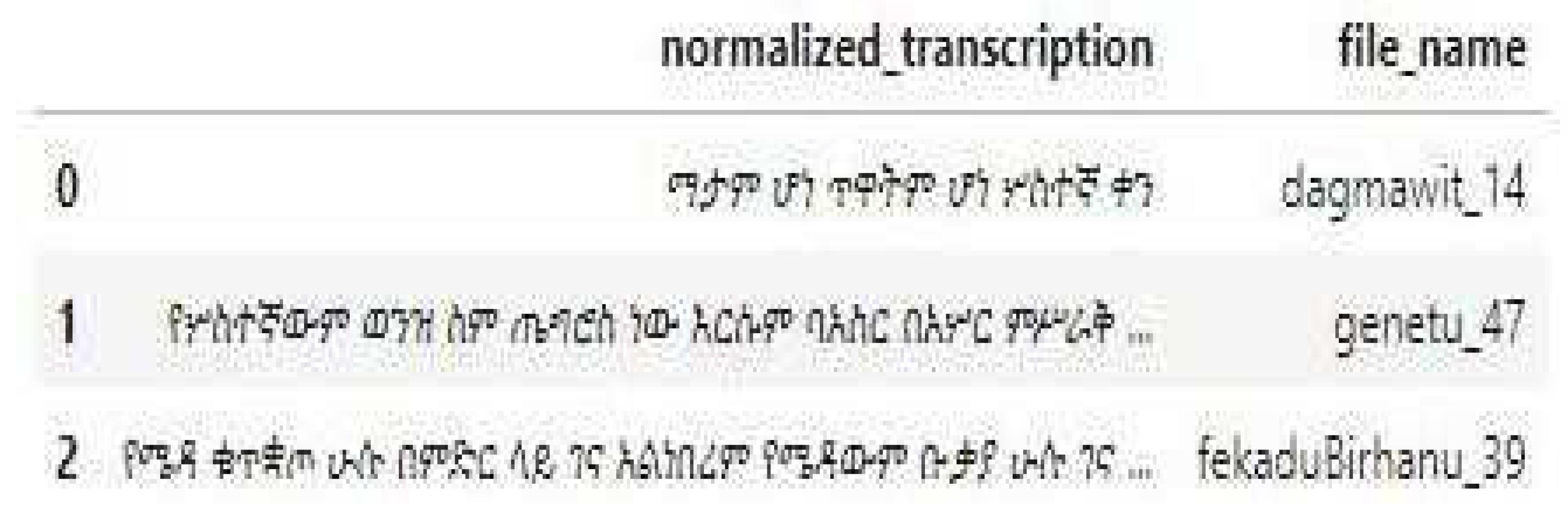
Figure 2.
Proposed architecture of the model.
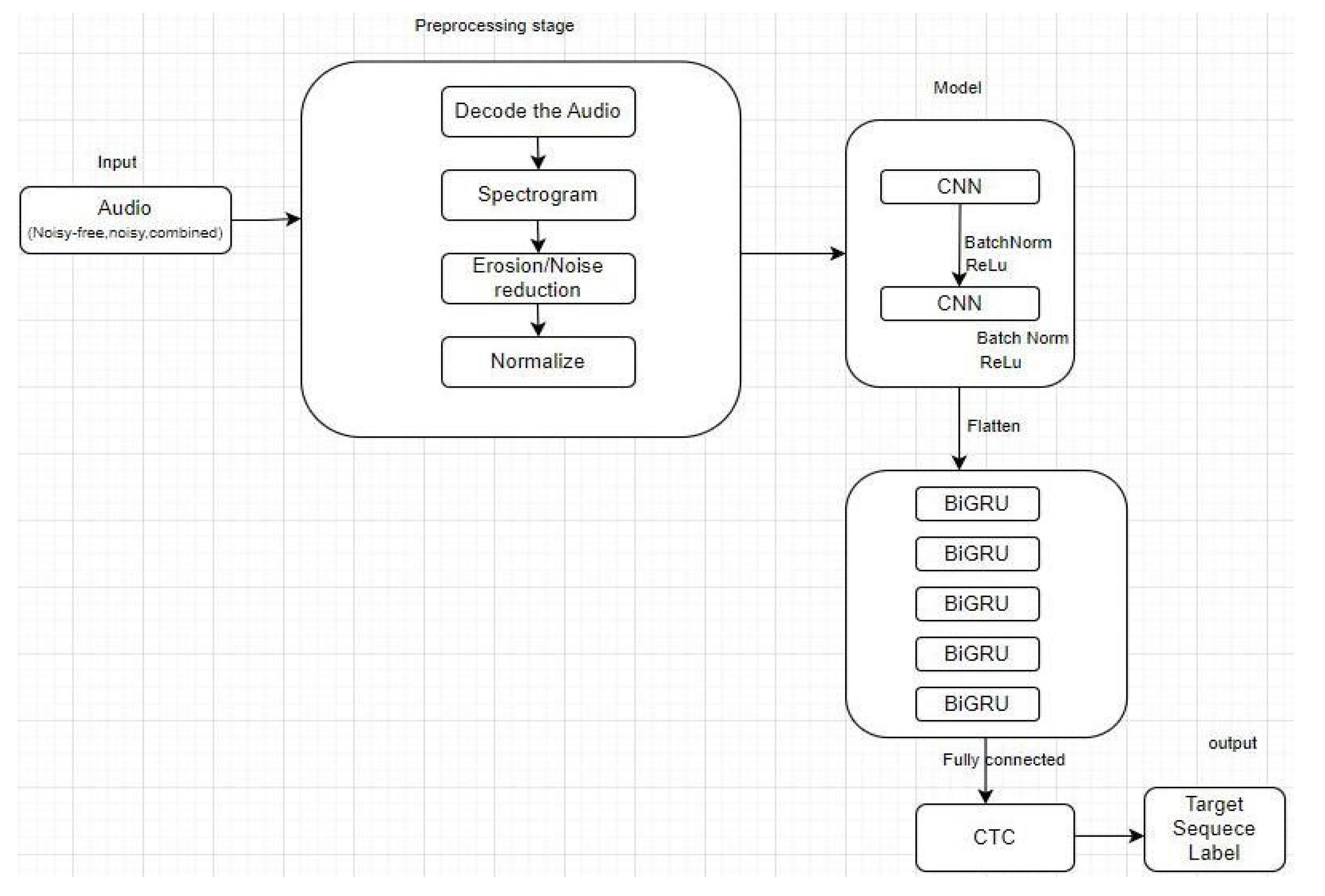
Figure 3.
Presents the loss function in a noisy data.
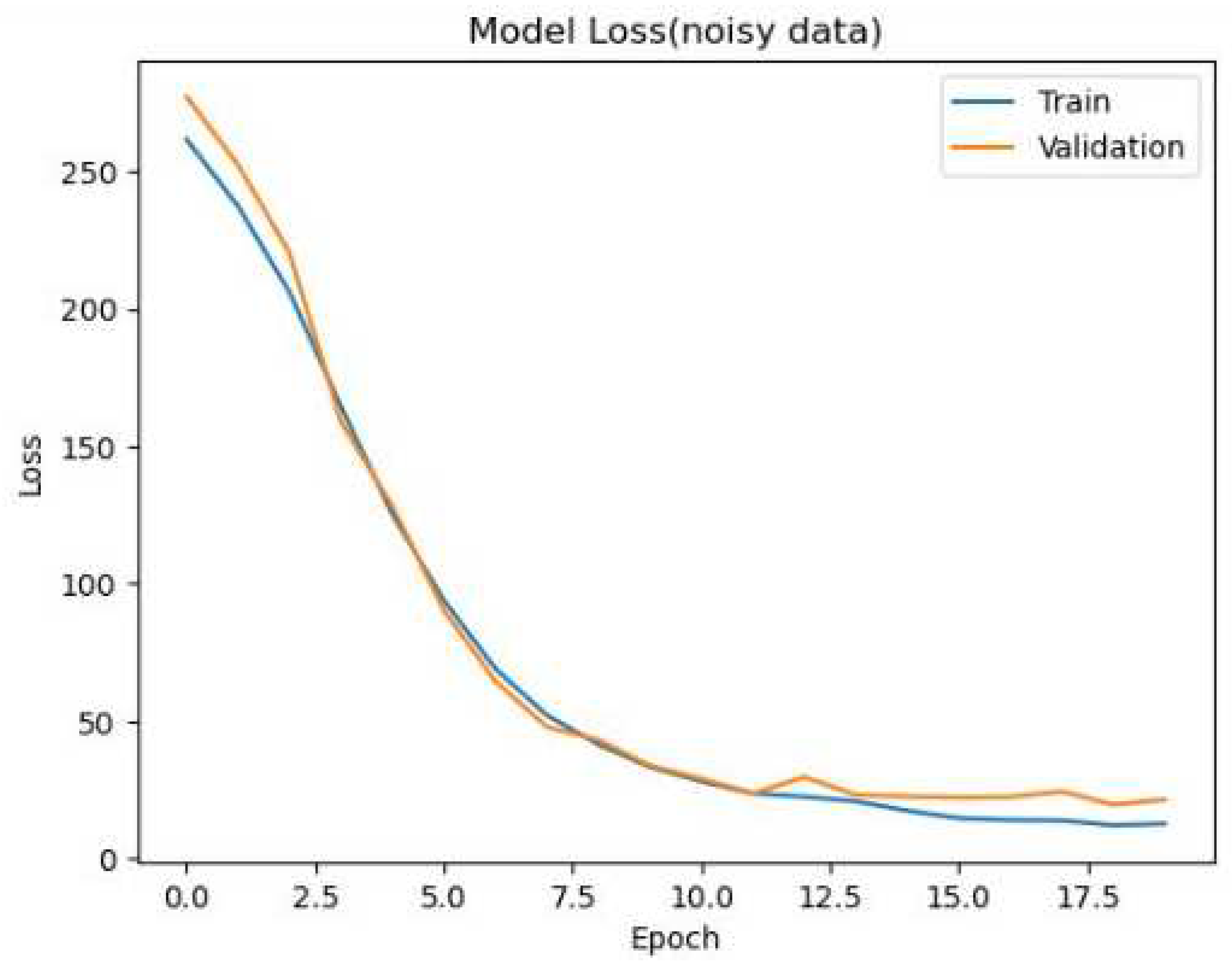
Figure 4.
WER for noisy data and the predictions for unseen validation data via RTX800 NVIDIA GPU.
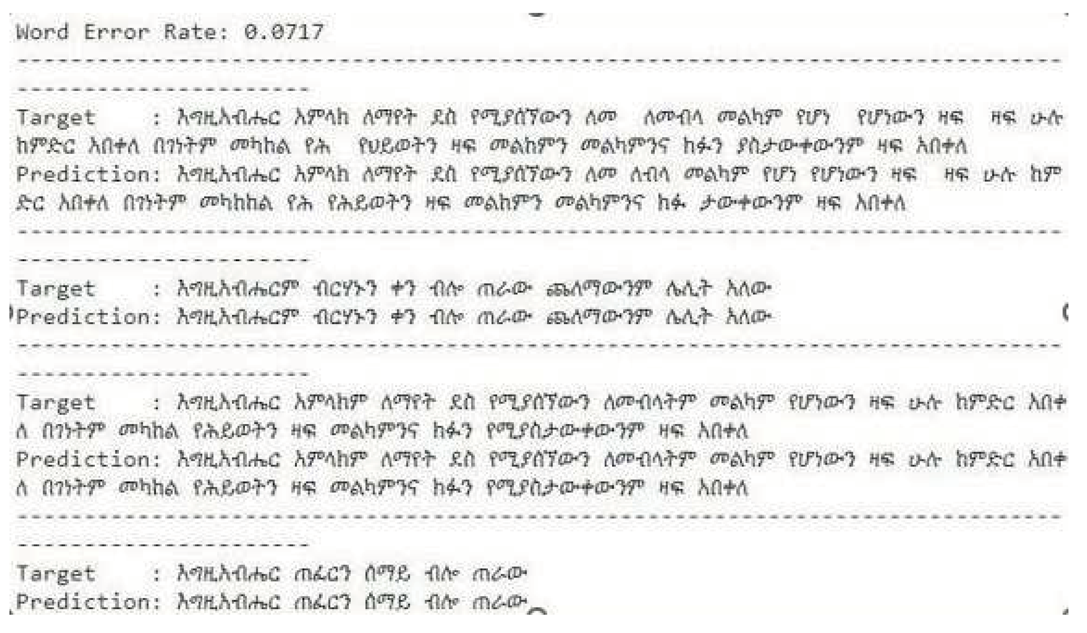

Table 1.
Presents the Word Error Rate (WER) results.
| Experiment | Noisy Data |
|---|---|
| Spectral Subtraction | WER = 8.5% |
| Subspace Filtering | WER =7.4% |
| Combined (Spectral+Subspace) | WER = 7% |
| Without Noise- reduction technique | WER = 10.5% |
Table 2.
Comparison of BIGRU and BILSTM.
| Model | WER (%) | Number of Parameters |
|---|---|---|
| BIGRU | 5 | 26,850,905 |
| BILSTM | 7 | 36,435,678 |
Disclaimer/Publisher’s Note: The statements, opinions and data contained in all publications are solely those of the individual author(s) and contributor(s) and not of MDPI and/or the editor(s). MDPI and/or the editor(s) disclaim responsibility for any injury to people or property resulting from any ideas, methods, instructions or products referred to in the content. |
© 2024 by the authors. Licensee MDPI, Basel, Switzerland. This article is an open access article distributed under the terms and conditions of the Creative Commons Attribution (CC BY) license (http://creativecommons.org/licenses/by/4.0/).
Copyright: This open access article is published under a Creative Commons CC BY 4.0 license, which permit the free download, distribution, and reuse, provided that the author and preprint are cited in any reuse.


