

Submitted:
13 February 2024
Posted:
13 February 2024
You are already at the latest version
Abstract
The aim of this research was to analyze the impact of implemented erosion control works (ECW) on soil erosion intensity in the watershed of the Ćelije reservoir (Rasina River) in the period between 1968 and 2022. The Erosion Potential Method was used to calculate the annual gross erosion (W), sediment transport (G), and erosion coefficient (Z) in the study area. As a result of the performed ECW there was a general decreasing trend in the intensity of soil erosion processes in the last 54 years. The specific annual gross erosion was 1189.12 m3/km-2/year-1 in 1968, while in 2022 it was 554.20 m3/km-2/year-1. The specific sediment transport was 540.18 m3/km-2/year-1 in 1968 and 253.55 m3/km-2/year-1 in 2022. Due to the changes in the intensity of erosion processes the specific annual gross erosion decreased by 634.92 m3/km-2/year-1, and the specific sediment transport by 286.63 m3/km-2/year-1. The erosion coefficient was reduced from Z=0.62 to Z= 0.35. A dependence between the slope of siltation and the natural bed slope was defined. The results show a significant correlation between erosion intensity and performed ECW, providing a basis for future watershed management and defining a strategy for soil erosion control in the Ćelije reservoir watershed.
Keywords:
soil erosion
; Erosion Potential Method
; erosion coefficient
; erosion control works
; sediment
; sediment transport
; slope siltation
1. Introduction
Soil erosion is the most widespread form of land degradation. Due to climate change increasing of erosion processes intensity is expected. Compared to other forms, water erosion causes the greatest losses of soil. The rate of soil erosion is primarily affecting by topography, precipitation, soil type, land use and land management practices [1,2,3,4].
Disturbances in watersheds due to deforestation, mining activities, construction of facilities and other infrastructure projects lead to dramatic erosion processes, increased soil loss and sediment transport into watercourses [5]. Sediment yield in river basins and sediment transport in watercourses represent two components of a global natural process that, due to its consequences, have significant ecological and hydrological importance.
The territory of Serbia is completely threatened by soil erosion of various intensities, with 36% of the territory affected by erosion processes categorized as excessive, intensive and medium intensity [6].
The reservoir Ćelije was formed in 1979 by constructing a dam 55 meters high in the Zlatarska Gorge (Rasina, right tributary of the Zapadna Morava). The initial purpose of the reservoir was flood protection, sediment retention, and irrigation, but later it began to be used for water supply. The reservoir Ćelije is a strategic part of the Rasina-Pomoravlje regional water supply system, which includes the downstream part of the Zapadna Morava River and the upstream part of the Velika Morava River.
The successful functioning of the reservoir over time has been significantly endangered by the reduction of the storage capacity due to sediment siltation [7]. In addition to reducing the storage capacity and water volume in the reservoir, erosion processes contribute to chemical pollution of water with materials of both natural and anthropogenic origin. Chemical substances of natural origin, resulting from the decay of rocks, are transported into the hydrographic network with sediment erosion. On the other hand, anthropogenic chemical pollution occurs due to the runoff of artificial fertilizers and pesticides from agricultural areas into river basins [8]. Due to erosion processes, many reservoirs in Serbia have been rapidly silted up with sediment and practically converted into sediment reservoirs. A typical example is the Zvornik reservoir on the Drina River, reservoirs on the Zapadna Morava River, and so on [9].
Soil erosion is the main cause of reservoir sedimentation, meaning that sedimentation is also a complex process that depends on numerous natural and anthropogenic factors [10,11]. Large number of research studies on erosion processes, sediment yield and transport in reservoir basins, indicating the significance of sediment issues [12].
Erosion and torrent control works in Serbia started at the end of 19th century, but not until 1907 as organized activity. Since then, a significant amount of erosion control works have been performed in the territory of Serbia up to the present day [13].
Properly designed and performed erosion control works cause the decrease of soil erosion intensity. In this respect, technical and biological works have different activities and effects. Biological works such as afforestation, reseeding, and orchard establishment on terraces are carried out on watershed slopes. Technical works can be longitudinal, for protection stream banks against erosion and sloughing and transversal for prevention of torrent beds erosion and retaining the sediment (primarily bedload) [14,15].
Multiple studies on the effects of erosion control works at the national, regional [16,17,18] and global levels, indicate their significance in reducing soil erosion intensity [19,20,21,22,23]. Technical works provide the desired results in a shorter time period, while biological and biotechnical works provide a long lasting solution to erosion and sedimentation issues within the watershed.
The effects of check dams are significant and studying them enables improvements and rationalization of erosion control works. By constructing check dams in their accumulation area, sediment is retained, forming a siltation behind the structure. The slope of the upper surface of siltation represents the slope of siltation, and practicall represent specific case of the equilibrium bed slope [24,25,26,27,28,29]. Field researches on the effects of check dams in Serbia shows that the best results in calculating the slope of siltation are based on the regional analytical dependence of the slope of siltation on natural bed slope.
The main aim of this research is to determine the spatial and temporal changes in soil erosion intensity and determine the effects of erosion control works on sediment yield, sediment transport and spatial distribution of soil erosion processes in the watershed of the Ćelije reservoir based on field researches in two time periods 1968 and 2022. The analysis of the effects of erosion control works is performed by comparing soil erosion intensity, sediment yield and transport before and after the works, as well as by calculating the amount of sediment retained upstream of the check dams and defining the slope of siltation.
2. Materials and Methods
2.1. Study Area
The Rasina River is a right tributary of the Zapadna Morava River, with a total watershed area of 981 km2. Rasina springs on the slopes of the Goč and Željin mountains at an elevation of 1340 meters above sea level, formed by the merging of the Velika and Burmanska river (Figure 1). The lowest elevation of the Rasina is 134 meters above sea level, at the confluence in Zapadna Morava five kilometers downstream from Kruševac. Up to the village of Razbojna, it flows through a canyon-like valley with small erosion enlargements, such as the one near Brus. Between Razbojna and Brus, it flows through a shallow and wide channel through the Dobroljubac basin, before entering the Zlatarska Gorge where it forms several entrenched meanders. The watershed is elongated with a developed hydrographic network. Apart from the Zagrža river, which is the left tributary, all other tributaries are from the right. All these rivers flow through canyon-like valleys with steep slopes transporting sediment. The largest among them are the Graševac River, coming from Kopaonik, and the Blatašnica River from Jastrebac.
The Rasina River drains the slopes of the Jastrebac and Kopaonik mountains, reaching elevations of 1500 meters above sea level and 1900 meters above sea level, respectively. According to the topographic map, the watershed area upstream of the dam is 609.15 km2. The perimeter of the watershed is 184.47 km. The river length is 69.95 km, and the length of the watershed is 49.39 km. The lowest elevation in the watershed is 239 meters above sea level at the dam profile, while the highest elevation is 1936 meters above sea level. The average elevation in the watershed is 695 meters above sea level, with a mean elevation difference of 447 meters. The average slope of the watershed is 34.65% (Table 1).
Slope angles up to 10 degrees cover 29% of the watershed area. Dominant slopes are between 10-25 degrees, covering 60% of the surface. Areas with slopes greater than 25 degrees constitute 11% (Figure 2a). Analysis of hypsometric characteristics of the Ćelije reservoir watershed area shows that 23% of the surface is located between 300 and 500 meters, 58% of the surface is between 500 and 1000 meters above sea level, and 18% is located above 1000 meters. Below 300 meters, there is only 1% (Figure 2).
These natural characteristics indicate a significant predisposition of the watershed area for the development of erosion processes, sediment yield and transport.
The geological composition of the Ćelije reservoir watershed is predominantly characterized by the following geological formations: Paleozoic bedrock complex (crystalline schists), Mesozoic bedrock complex (flysch), Paleogene bedrock complex, Neogene bedrock complex, and Quaternary deposits.
According to the resistance to erosion processes, bedrocks are categorized into four categories: very solid rocks, conditionally solid rocks, conditionally erodable rocks, and very erodable rocks. Conditionally solid are present on 13.75% of the area, conditionally erodable rocks on 38.27%, and very erodable rocks on 44.88%, meaning that more than 90% of the area is potentially threatened by erosion (Figure 3b).
The dominant soil types in the watershed are of weaker structure. The most prevalent soil types are eutric cambisols (35%), followed by distric cambisols (12.8%), ranker eutric soils (8.7%), ranker distric soils (6.6%), and regosol (7.5%), while other soils are present on smaller areas (Figure 3а).
The lowland part of the Rasina River watershed is characterized by a moderately continental climate, while the hilly-mountainous area of the watershed has uneven elevation influenced by the continental climate.
For the purpose of determining the climatic characteristics of the Ćelije reservoir watershed area for the period from 1990 to 2022 (Table 2), data from meteorological stations in Kruševac, Brus, Blace, Goč, Kopaonik, and Jastrebac were used [30].
The annual precipitation during the period from 1946 to 1990 at the Kruševac meteorological station was 649 mm, while at the Brus meteorological station it was 678 mm, indicating that the precipitation amount was higher by 89 mm and 144 mm respectively (Figure 4a).
Analyzing the data from the "Kruševac" meteorological station, the average annual temperature for the lower part of the watershed is 12.4°C. For the mountainous part of the watershed, the average annual temperature is 4.2°C, based on data from the "Kopaonik" meteorological station at 1710 m above sea level (Figure 4b).
Comparing to the values for the period 1946 - 1990, the average annual temperature at the Kruševac meteorological station has increased by 1.4 degrees Celsius.
The Rasina River exhibits all the characteristics of a torrential watercourse because its flow amplitudes are very pronounced. In April, it has 5.5 times more water than in August. The highest flow occurred in April 1958 and amounted to 342 m3/s.
2.2. Methodology
There is a large number of erosion risk assessment models in use today [32,33,34]. The selection of a specific model largely depends on the purpose of the research, data availability, time and finances required for the project. Most models used in soil erosion studies are empirical models. These models vary in complexity and incorporate different techniques and approaches to define erosion intensity, sediment yield and transport [35,36,37,38].
The Erosion Potential Method (EPM) also known as Gavrilović was developed and calibrated using field research in the Juzna Morava River basin [39,40,41,42,43,44]. This method is widely used in Serbia, the former Yugoslav republics [45,46,47,48,49], as well as in the Mediterranean region, Central Europe, the Middle East, and other climates [50,51,52,53,54,55,56,57].
Method has provided reliable results for evaluating of intensity of soil erosion processes, mean annual soil erosion rate and sediment transport and implementing erosion control measures.
The biggest challenge lies in verifying the obtained data. At the regional and broader levels, reliable data for comparing estimated and actual soil loss practically do not exist. The method involves both qualitative and quantitative analyses and is adapted to GIS environments. The erosion mapping procedure includes processing various datasets and calculating numerical indicators.
The basic premise of the method is to reduce subjective errors in coefficient estimation to an acceptable level, and the development and improvement of the method are aimed at eliminating them.
The EPM involves classifying the intensity of erosion into 5 categories, from very slight (V category) to excessive (I category). The primary parameter used to classify the intensity and category of erosion in this method is the erosion coefficient (Z).
Parameters for determining the erosion coefficient include topographic, geological and pedological characteristics, land use practices within the watershed, and the degree of erosion vulnerability of the watershed. Each of these parameters can be represented by a digital map and by overlaying these maps a separate composite map is generated, where areas with identical coefficient values are formed. For each of these areas, the average slope of the terrain is determined, and all these data represent input values for calculating the erosion coefficient (Z) according to the following Equation (1):
where X represents soil protection coefficient; Y is the ceofficient of soil resistance; φ is the erosion and stream network development coefficient, while I is the average slope of the watershed.
The values of coefficients used in the EPM are in Table 3.
Precipitation and temperature data were obtained from 6 meteorological stations for the period 1990 to 2022. The coefficient Y was determined based on a geological map at a scale of 1:100,000. Coefficients X and ϕ were determined using orthophotos, satellite imagery, and field research of erosion conditions during 2022, based on which a land use map was created. Different land use categories were identified, harmonized for both periods.
Morphometric characteristics and slopes were determined using a topographic map at a scale of 1:25,000 and digital elevation model (SRTM).
The calculated values for each delineated area form the basis for the classification of erosion processes. The coefficient values (Z) are categorized into five classes, which provide an optimal number for graphical representation of the erosion status and surface prevalence (Table 4). For practical application and calculations, each category has been assigned a qualitative name and corresponding mean value for the erosion coefficient (Z). This erosion map thus created serves as the foundation for further application in other areas.
The described procedure resulted in the creation of an erosion map for the entire analyzed area. Data on the surface prevalence of erosion, defined by the mentioned method, serve as the initial basis for calculating sediment tield and transport from the watershed area. These data have enabled the development of new methods for calculating sediment transport.
The calculation of specific annual gross erosion was performed according to the following Equation (2)
where, Wsp is specific annual erosion (m3/km-2/year-1), T is the temperature coefficient, H is mean annual precipitation (mm), Z is the erosion coefficient and F is the basin area (km2)
Temperature coefficient (T) is calculated by Equation (3):
where t is mean annual temperature (°C)
The annual gross erosion for the entire watershed area (Wyear) is calculated by multiplying the watershed area (F) by the specific annual gross erosion (W) by Equation (4).
Having calculated the total annual soil erosion rates, we calculated the sediment delivery ratio, which is needed for the actual sediment yield calculation. Gavrilovic [42] suggested the following Equation (5) for the determination of the sediment delivery ratio Ru:
where O is perimeter of watershed (km), D is average distance of elevation of the watershed (km) and L is length of the watershed (km).
Specific sediment transport is calculated as:
The actual sediment transport is:
In this study, erosion mapping was based on the Erosion Potential Method successfully integrated into the GIS environment, using the open-source geographic information system QGIS [57]. To define the change in soil erosion intensity, GIS was used to overlay the erosion map from 1968 with the current erosion map from 2022. The modeling, digitization, and mapping were conducted using QGIS 3.32.0.
3. Results
3.1. Analisys of Performed Erosion Control Works (ECW) in the Study Area
3.1.1. Transverse structures in Torrential Streams (Check dams)
In the Rasina River watershed in the immediate vicinity of the reservoir as well as upstream of the reservoir technical erosion control works were actively undertaken to retain the bedload and stabilize torrential channels. These works accompanied the period of dam construction, and continued even after the dam was built and reservoir filled.
Between 1972 and 1990, over thirty check dams were constructed (Figure 6), primarily using concrete or stone in cement mortar. A significant number of these structures are still evident in the field. For the purposes of this research, 14 check dams built within the channels of 6 streams were analyzed, representing the entire basin by their characteristics. Ten of these barriers were made of stone in cement mortar (Blatašnica, Žunjska River, Zagrža and Rasina), while four were constructed from concrete (Koznička and Popovačka River).
The check dams constructed within the channels of torrential streams serve multiple purposes: to retain sediment and to decrease bed slope. Reducing the bad slope of the watercourse also implies a reduction in the transport capacity for sediment (Table 5).
The amount of sediment retained upstream of the check dams depends on the effective height of check dams, the valley geometry upstream of check dams, and the slope of siltation. The quantity of the retained sediment is calculated using the Kitin 1975 formula [58]:
where W is the volume of the retained sediment in the silting-up area (m3), m is mean width of the silting-up area (m), hk - dam effective height (m), It is natural torrent bed slope in decimal form, Iz is slope of siltation in decimal form.
The input parameters in the formula were measured for each check dam directly in the field.
The calculation results indicate that check dam 1 on the Koznicka River retained the highest amount of sediment, which is logical considering the geometric characteristics of the channel upstream of check dam. In comparison with this check dam, check dam 2, which has a greater effective height, retained much less sediment, primarily due to unfavorable geometric characteristics (large bed slope of the channel upstream of the check dam and narrow width).
Based on field research it was concluded that all check dams in the watershed have fulfilled their function: they retained the maximum amount of sediment, stabilized the river bed, and reduced the bed slope. The siltation upstream of the check dams are covered with vegetation.
Considering that these check dams were constructed with pupose of protecting the Ćelije reservoir from sedimentation, which is a large-scale water management facility with significant investment value, there is no need for a separate economic analysis to conclude that these check dams have justified the construction costs. It should be noted that no technical works have been carried out since the 1990s. The existing structures are not adequately maintained, and many of them are damaged.
3.1.2. Biological Works
In addition to technical erosion control works, activities related to afforestation and grassing have been carried out every year.
During the period from 1960 to 1980, an annual afforestation of about 100 to 150 hectares was carried out on these surfaces, resulting in afforestation of approximately 2,000 to 3,000 hectares for this period. In the Žunjska River basin, 150 hectares were afforested with black pine. From 1980 to 1988, a total of 1,221 hectares were afforested, and after the year 2000, an average of 50 hectares were afforested annually.
Based on available data on afforestation works, it can be estimated that 5,000 hectares have been afforested in the last 54 years. The tree species used for afforestation include spruce, white pine, black pine, acacia, poplar, red oak, douglasia, larch, and Scots pine (Figure 7).
In parallel with afforestation activities, distribution of grass seeds to the local population was carried out to establish artificial pastures, thus preventing soil erosion.
The grass mixture was suitable for these terrains both in terms of soil and altitude. In most cases, the mixture consisted of the following grass species: Dactylis glomerata (orchard grass), Festuca pratense (meadow fescue), Festuca rubra (red fescue), Lolium multiflorum (Italian ryegrass), Lolium perenne (perennial ryegrass), Phleum pratense (timothy grass), and legumes: Trifolium pratense (red clover) and Lotus corniculatus (bird's-foot trefoil).
Based on available data, it can be estimated that around 4000 hectares were seeded with grass.
3.2. Land Use before and after ECW
According to data from the 1968, before the construction of the dam and the formation of the reservoir, forests covered 33.05% of the watershed. Meadows and pastures accounted for 26.84% of the area (Table 6). Arable land covered 18.92% of the watershed. Areas under degraded forest accounted for almost 16%. Settlements comprised 4.22% of the territory. Barren land made up 1% of the territory (Figure 8a).
According to data from the land use map from 2022, forests cover 63.07% of the watershed area. Mostly, these are deciduous forests (56%), while coniferous forests cover 5% of the area. Degraded forests account for 8.96%. Meadows and pastures make up almost 11% of the watershed area. Arable land covers 13.78% and is located along the Rasina River and at higher altitudes in settlements. Settlements occupy 2.38% of the area. Barren land covers 0.3% of the territory (Figure 8b).
3.3. Spatial Distribution of Erosion Coefficient (Z), Specific Annual Gross Erosion (W) and Specific Sediment Transport (G) before and after ECW
According to the erosion map for the Zapadna Morava watershed created in 1968, before the construction of the dam and the formation of the Ćelije reservoir, 9% of the watershed area was extremely endangered by erosion (Table 7). All categories of erosion were represented except for very weak erosion. Intensive erosion covered 28.56% of the watershed area, while medium and weak erosion were present on 31.42% and 31.04% of the watershed area, respectively. With a mean erosion coefficient of 0.62, the watershed area was affected by intensive erosion processes, indicating that the erosion intensity in the watershed was in the 3rd category (Figure 9a).
According to the erosion map for the year 2022, the area under excessive erosion is almost negligible, with intensive erosion covering 0.54% of the area. Medium erosion is present on 23.82% of the area. Weak erosion dominates, covering 38.66% of the area, while very weak erosion is present on 6.98% of the area. The erosion coefficient is 0.35, indicating that the erosion intensity in the watershed is in category 2 (Figure 9b).
Specific annual gross erosion was approx. 1189 m3/km-2/year-1 in 1968 and approx. 540 m3/km-2/year-1 in 2022, while specific sediment transport into the reservoir was approx. 554 m3/km-2/year-1 in 1968 and approx. 254 m3/km-2/year-1 in 2022 (Table 8).
Total annual gross erosion was approx. 724352 m3/year in 1968 and approx. 337590 m3/year in 2022, while total sediment transport into the reservoir was approx. 329000 m3/year in 1968 and approx. 154500 m3/year in 2022 (Table 9).
4. Discussion
The results of erosion control works performed in the Celije reservoir watershed is decreasing in the intensity of erosion, sediment production, and transport during the observed period. Biological works have altered the land use pattern in the watershed, impacting the intensity of erosion processes. Before the implementation of erosion control works in the watershed, the distribution of land use was as follows: forests covered 33.05% of the area. Meadows and pastures occupied 26.84% of the area. Arable land accounted for 18.92% of the watershed. Degraded forests comprised 16% of the area. Settlements covered 4.22% of the area. Barren lands accounted for 1% of the area. According to the status as of 2022, the distribution of land use has changed significantly: forests now cover nearly two-thirds (63.07%) of the watershed. Meadows and pastures occupy 11% of the area. Arable land is present on 13.78% of the watershed. Degraded forests now cover 8.96% of the area. Settlements occupy 2.38% of the watershed. Barren lands account for 0.3% of the area.
The change in land use structure has led to a reduction in the intensity of erosion processes. The specific annual gross erosion in the Celije reservoir watershed was 1189.12 m3/km-2/year-1 in 1968, while in 2022 decreased to 554.20 m3/km-2/ year-1. Similarly, the specific sediment transport was 540.18 m3/km-2/year-1 in 1968 and decreased to 253.55 m3/km-2/year-1 in 2022. Due to the change in erosion process intensity in the watershed, the specific sediment production decreased by 634.92 m3/km-2/year-1, and the specific sediment transport decreased by 286.63 m3/km-2/year-1. The value of the erosion coefficient decreased from Z=0.62 in 1968 to Z=0.35 in 2022.
According to the erosion map for 2022, areas with excessive, strong, and moderate erosion are less prevalent, while more areas are categorized as 4 and 5. In 1968, excessive and strong erosion covered 37.55% of the area, while in 2022, they only covered 0.54%.
The effects of biological and biotechnical structures were more noticeable in later periods. Reforestation works are considered most effective in reducing erosion intensity. The dependence of erosion coefficient reduction on the percentage of areas treated with biological works is significant, as these works directly affect changes in land use, thereby reducing erosion intensity [25].
The constructed technical objects provided certain favorable effects immediately after the construction (formation of siltation and sediment retention; reduction of bed slope; stabilization of banks). Analyzing the effects of dams from the perspective of retained sediment quantity showed that the greatest effect is achieved by selecting the appropriate location for constructing the object. Dams of the same effective height yield different effects depending on the valley width and bed slope.
The formed slope of siltation significantly influences the effects of dams. If the ratio of slope of siltation to natural bed slope is close to one, the silting up area is longer, and therefore the amount of retained sediment is greater (Figure 10).
Based on the research results, a statistical analysis was conducted to determine the relationship between the natural bed slope and the measured slope of siltation. The natural bed slope was defined based on the project documentation, while the slope of siltation was defined in the field. The Pearson`s correlation coefficient is 0.965, indicating a high correlation between the parameters. The coefficient of determination value explains 93.1% of the total variation. The dependence of the slope of siltation on the natural bed slope is represented by a linear regression Equation (9) in which the parameters are significant at the given level of significance:
Iz = 0,759 It - 0.794
The Equation (9) cannot be applied for values of the natural bed slope less than 1.046% because negative values of the slope of siltation are obtained. It has a regional character and can be applied in torrential streams with similar natural characteristics.
In addition to the implemented erosion control measures, demographic changes in the watershed also had a significant impact on reducing soil erosion intensity, primarily due to the decrease in population and unfavorable age structure. According to the 2022 census data, the population in settlements within the watershed has decreased by 41% compared to 1953. All of this has led to a reduction in agricultural production, resulting in the formation of grassland and forest cover on abandoned fields and orchards through the spontaneous growth of vegetation. This vegetation cover positively contributes to mitigating erosion processes. Due to the influence of the reservoir within the watershed, there are no major issues with flash floods.
However, despite research results showing that the erosion intensity in the watershed is satisfactory, it is important to consider that the physical characteristics, geological, and pedological substrate of the watershed make it highly susceptible to erosion processes. Also according to research, climate change from 1961 until today has shown significant changes in temperature and the distribution and quantity of precipitation [59].
As for the entire territory of Serbia, in this area is also problem the lack of implementation of erosion control measures and maintenance of existing structures since the early 1990s, caused by the economic crisis.
Erosion control management was implemented 50 years ago, but the approach to erosion protection has changed in the meantime, primarily due to a lack of financial resources, leading to inadequate implementation of erosion control measures. On a smaller portion of arable land, there are areas where erosion control practices are applied, but there are also areas where this principle is compromised, leading to an intensification of erosion processes.
5. Conclusions
The Ćelije reservoir was created in 1979 by building a dam on the Rasina River in the Zlatar Gorge. Significant erosion control works were carried out to protect the reservoir from sedimentation in the watershed. Research shows that these works have significantly reduced erosion intensity in the watershed, sediment production and transport to the reservoir, thereby extending the use of the reservoir.
The relationship between slope of siltation and natural bed slope obtained through research can be utilized in the design of projects within the study area, as well as in watersheds with similar natural characteristics.
Based on the current state, it may appear that erosion issues in the watershed have been minimized. However, the natural characteristics of the watershed make it highly susceptible to erosion processes. While erosion control management was implemented over 50 years ago, the approach to erosion protection has changed since the 1990s due to a severe economic crisis in Serbia, leading to reduced financial resources and inadequate implementation of erosion control measures. Maintenance of existing structures and the repair of damaged ones have also been neglected for the same reasons.
Considering the significance of the Ćelije reservoir for water supply, it is essential to continue with erosion control works and measures in the watershed. This is necessary not only to reduce the amount of sediment entering the reservoir but also to prevent chemical and mechanical pollution that affects water quality.
Author Contributions
Conceptualization, I.S., N.D. and R.R.; methodology, I.S.; validation, J.C.; formal analysis, I.S. and N.Z.; investigation, I.S. and M.S.; resources, I.S., J.C. and M.S.; data curation, I.S.; writing—original draft preparation, I.S.; writing—review and editing, R.R., N.D., M.S. and J.C.; visualization, I.S. and N.Z.; supervision, R.R. All authors have read and agreed to the published version of the manuscript.
Data Availability Statement
Data are contained within the article.
Conflicts of Interest
The authors declare no conflict of interest.
References
- Panagos, P.; Borrelli, P.; Poesen, J.; Ballabio, C.; Lugato, E.; Meusburger, K.; Montanarella, L.; Alewell, C. The new assessment of soil loss by water erosion in Europe, Environmental Science & Policy, 2015, Volume 54, p p. 438-447. [CrossRef]
- Borrelli, P.; Robinson, DA.; Panagos, P.; Lugato E, Yang JE, Alewell C, Wuepper D, Montanarella L, Ballabio C. Land use and climate change impacts on global soil erosion by water (2015-2070)., Proc Natl Acad Sci U S A. 2020 Sep 8;117(36):21994-22001. Epub 2020 Aug 24.PMID: 32839306. [CrossRef]
- Zhiying Li; Haiyan Fang: Impacts of climate change on water erosion: A review, Earth Science Reviews, December 2016, Volume 163, pp. 94-117. [CrossRef]
- Manojlović, S.; Sibinović, M.; Srejić, T., Novković, I.; Milošević, MV.; Gatarić, D.; Carević, I., and Batoćanin, N. Factors Controlling the Change of Soil Erosion Intensity in Mountain Watersheds in Serbia. Front. Environ. Sci. 2022, 10:888901. [CrossRef]
- Ristić R.; Radić B.; Vasiljević N.; Nikić Z. Land use change for flood protection – A prospective study for the restoration of the river Jelašnica watershed, Bulletin of the Faculty of Forestry 2011, 103: 115-130. [CrossRef]
- Ristić, R.; Kostadinov, S.; Abolmasov, B.; Dragićević, S.; Trivan, G.; Radić, B.; Trifunović, M.; and Radosavljević, Z. Torrential floods and town and country planning in Serbia, Nat. Hazards Earth Syst. Sci., 2012, 12, pp 23–35. [Google Scholar] [CrossRef]
- Juško, V.; Sedmák, R.; Kúdela, P. Siltation of Small Water Reservoir under Climate Change: A Case Study from Forested Mountain Landscape ofWestern Carpathians, Slovakia. Water 2022, 14, 2606. [Google Scholar] [CrossRef]
- Kostadinov, S.; Dragovic, N.; Zlatic, M.; Todosijevic, M. Erosion control works and the intensity of soil erosion in the upper part of the river Toplica drainage basin. Earth Environ. Sci. 2008, 4, 012040. [Google Scholar] [CrossRef]
- Kostadinov, S.; Milovanović I.; Dragovic, N.; Todosijevic M. Soil erosion in the drenage basin of the river Rasina upstream of the reservoir Celije, International Scientific Conference Forest Ecosistems and climate changes, Belgrade, 2010, Proceedings Volume 1, ISBN 978-86-80439-22-8, p 237-242.
- Obialor, C.; A., Okeke, O.; C., Onunkwo A. A.; Fagorite, V. I.; and Ehujuo, N. N. Reservoir sedimentation: causes, effects and mitigation International Journal of Advanced Academic Research | Sciences, Technology and Engineering 2019| ISSN: 2488-9849 Vol. 5, Issue 10.
- Drobnjak A.; Zlatanović N.; Milovanović I.; Čotrić J. Comparative Analysis of Methods for Estimation of Reservoir Siltation Intensity at the Gvozdac Lake Reservoir in Serbia, IWA 6th Eastern European Young Water Professionals Conference „East meets West“,Istanbul, Turkey, 28-30 May 2014, Organised by: IWA, UNESCO-IHP Institute for Water Education and Istanbul Technical University, Proceedings (CD) pp. 88-92, 2014.
- Dutta, S. Soil erosion, sediment yield and sedimentation of reservoir: A review. Model. Earth Syst. Environ. 2016, 2, 123. [Google Scholar] [CrossRef]
- Kostadinov, S.: Erosion and torrent control in Serbia: hundred years of experiences, International Conference: Erosion and Torrent Control as a Factor in Sustainable River Basin Management, Belgrade, Serbia, 25–27 September 2007, Proceedings (CD), 2007.
- Kostadinov, S.; Marković, S. Soil erosion and effects of erosion control works in the torrential watersheds in south-east Serbia. In Erosion and Sediment Yield: Global and Regional Perspectives; Walling, D.E., Webb, B.W., Eds.; IAHS Press: Walingford, UK, 1996; pp. 321–332. ISSN 0144-7815. [Google Scholar]
- Shakeel Ahmad Bhat; Mehraj U. Din Dar and Ram Swaroop Meena Soil Erosion and Management Strategies, Springer Nature Singapore Pte Ltd. 2019, 73 R. S. Meena et al. (eds.), Sustainable Management of Soil and Environment. [CrossRef]
- Kostadinov, S.; Dragovic, N.; Zlatic, M.; Todosijevic, M. Erosion control works and the intensity of soil erosion in the upper part of the river Toplica drainage basin. Earth Environ. Sci. 2008, IOP Conf. Ser.: Earth Environ. Sci. 4 012040. [CrossRef]
- Stanimir Kostadinov; Sonja Braunović; Slavoljub Dragičević; Miodrag Zlatić; Nada Dragović; Nikola Rakonjac Effects of Erosion Control Works: Case Study-Grdelica Gorge, the South Morava River (Serbia) Water 2018, 10(8), 1094. [CrossRef]
- Milovanovic, I.; Cotric, J.; Stefanovic, M.: Analysis of the impact of applied antierosion works on reducing siltation in the reservoir “Celije“ Forum Geografic S.C.G.P.M., pp. 849-855., 2011.
- Ivan Blinkov; Alexandar Trendafilov Effects Of Erosion Control Work In Some Torrents In The Republic Of Macedonia, Conference on Water Observation and Information System for Decision Support , BALWOIS 2004 Ohrid, FY Republic of Macedonia, 25-29 May 2004.
- Petr Karásek; Jan Szturc; Josef Kučera; Jana Podhrázská; Jana Konečná Causes of Water Erosion and Benefits of Antierosion Measures in Model Locality Starovice – Hustopeče (South Moravia Region, Czech Republic), J. Ecol. Eng. 2019; 20(2):95-105. [CrossRef]
- Antonio Minervino Amodio; Dario Gioia; Maria Danese; Nicola Masini; Canio Alfieri Sabia Land-Use Change Effects on Soil Erosion: The Case of Roman “Via Herculia” (Southern Italy)—Combining Historical Maps, Aerial Images and Soil Erosion Model, Sustainability 2023, 15(12), 9479. [CrossRef]
- Panagos, P.; Borrelli, P.; Meusburger, K.; Van der Zanden E.H.; Poesen J.; Alewell, C. 2015d. Modelling the effect of support practices (P-factor) on the reduction of soil erosion by water at European Scale. Environmental Science & Policy 51, 23–34. [CrossRef]
- Xu, Y.; Yang, X.; Xu, G.; Fu, J.; Cai, S.; Mu, X.; Zhou, T.; Zhang, W.; Chen, J.; Li, L.; et al. Assessment of Integrated Soil and Water Conservation Practices on Soil Erosion Risk in a Typical Red-Beds Watershed in South China. Water 2023, 15, 2613. [Google Scholar] [CrossRef]
- Kostadinov, S.; Dragović, N.; Zlatić, M.; Todosijević, M. Natural effect of classical check dams in the torrents of the river Toplica drainage basin, Fresenius Environmental Bulletin, 20(4), Parlar scientific publication, Germany, 2011, p.p.1102-1108, ISSN: 1- 4619.
- Braunovic, S. Effects of Erosion Control Works on the State of Erosion in Grdelicka Klisura and Vranjska Kotlina. Ph.D. Thesis, University of Belgrade, Belgrade, Serbia, 4 October 2013. (In Serbian). [Google Scholar]
- Radonjic, J. Hydrologic and Psamologic Effects of erosion control works on the torrential sub-basina of the South Morava. Ph.D. Thesis, University of Belgrade, Belgrade, Serbia, 2018. (In Serbian). [Google Scholar]
- Todosijević M. Effects of transversal structures in the torrents of Drina river drainage basin in the sector of Loznica –Bacevci, Belgrade, Serbia, (Master of Science thesis, Faculty of Forestry, Belgrade), 2005. (In Serbian).
- Velojić M. Research of transversal structures effects in the torrents of Nisava river drainage basin), Belgrade, Serbia, (Master of Science thesis, Faculty of Forestry, Belgrade) 2000 (In Serbian).
- Kostadinov S. Analisys of the Effects of Classical and Filtration Check Dams in the Torrents of Serbia, Proceedings of the XXVI IECA Conference, Feb. 28th - March 3rd, 1995, Atlanta, pp. 111-124.
- Republic Hydrometeorological Service of Serbia. Available online: https://www.hidmet.gov.rs/ciril/meteorologija/klimatologija_godisnjaci.php.
- Statistical Office of Republic of Serbia, 2022 Census of Population, https://popis2022.stat.gov.rs/sr-Latn.
- Borrelli, P.; Alewell, C.; Alvarez, P.; Anache, J.A.A.; Baartman, J.; Ballabio, C.; Bezak, N.; Biddoccu, M.; Cerd`a, A.; Chalise, D.; Chen, S.; Chen, W.; De Girolamo, A.M.; Gessesse, G.D.; Deumlich, D.; Diodato, N.; Efthimiou, N.; Erpul, G.; Fiener, P.; Freppaz, M.; Gentile, F.; Gericke, A.; Haregeweyn, N.; Hu, B.; Jeanneau, A.; Kaffas, K.; Kiani-Harchegani, M.; Villuendas, I.L.; Li, C.; Lombardo, L.; Lopez - Vicente, M.; Lucas-Borja, M.E.; Marker, M.; Matthews, F.; Miao, C.; Mikos, M.; Modugno, S.; Moller, M.; Naipal, V.; Nearing, M.; Owusu, S.; Panday, D.; Patault, E.; Patriche, C.V.; Poggio, L.; Portes, R.; Quijano, L.; Rahdari, M.R.; Renima, M.; Ricci, G.F.; Rodrigo-Comino, J.; Saia, S.; Samani, A.N.; Schillaci, C.; Syrris, V.; Kim, H.S.; Spinola, D.N.; Oliveira, P.T.; Teng, H.; Thapa, R.; Vantas, K.; Vieira, D.; Yang, J.E.; Yin, S.; Zema, D.A.; Zhao, G.; Panagos, P. Soil erosion modelling: a global review and statistical analysis. Sci. Total Environ. 2021 14 6494. [CrossRef] [PubMed]
- De Vente, J.; Poesen, J. Predicting soil erosion and sediment yield at the basin scale: scale issues and semi - quantitative models. Earth - Sci. Rev. 2005 71, pp. 95–125. [CrossRef]
- De Vente, J.; Poesen, J.; Verstraeten, G.; Govers, G.; Vanmaercke, M.; Van Rompaey, A.; Arabkhedri, M.; Boix-Fayos, C. Predicting soil erosion and sediment yield at regional scales: where do we stand? Earth-Science Rev. 2013 127, 16-29. [CrossRef]
- Kamal Elbadaoui; Soukaina Mansour; Mustapha Ikirri; Kamal Abdelrahman; Tamer Abu-Alam and Mohamed Abioui Integrating Erosion Potential Model (EPM) and PAP/RAC Guidelines for Water Erosion Mapping and Detection of Vulnerable Areas in the Toudgha River Watershed of the Central High Atlas, Morocco, Land 2023, 12, 837. [CrossRef]
- Christos G. Karydas; Panos Panagos ; Ioannis Z. Gitas A classification of water erosion models according to their geospatial characteristics, International Journal of Digital Earth, 2014 7:3, 229-250. [CrossRef]
- C. Bosco; D. de Rigo; O. Dewitte; J. Poesen; P. Panagos Modelling soil erosion at European scale: towards harmonization and reproducibility, Nat. Hazards Earth Syst. Sci., 2015 15, pp. 225-245, www.nat-hazards-earth-syst-sci.net/15/225/2015/. [CrossRef]
- Efthimiou N., Lykoudi E., Karavitis C. 2017. Comparative analysis of sediment yield estimations using different empirical soil erosion models. Hydrological Sciences Journal. Vol. 62 p. 2674-2694. [CrossRef]
- Gavrilovic, S. A method for estimating the average annual quantity of sediments according to the potency of erosion. Bull. Fac. For. 1962, 26, pp. 151–168. [Google Scholar]
- Gavrilovic, S. Modern ways of calculating the torrential sediment and erosion mapping. In Erosion, Torrents and Alluvial Deposits; Yugoslav Committee for International Hydrological Decade: Belgrade, Serbia, 1970; pp. 85–100. [Google Scholar]
- Gavrilovic, Z. Use of an Empirical Method Erosion Potential Method for Calculating Sediment Production and Transportation in Unstudied or Torrential Streams, International Conference on River Regime. Hydraulics Research Limited, Wallingford, Oxon UK 1988 pp. 411-422.
- Gavrilović, S. Engineering of Torrents and Erosion. J. Constr. Spec. Issue 1972, 1–292. (In Serbian).
- Luca Milanesi; Marco Pilotti; Alberto Clerici; Zoran Gavrilovic Application of an improved version of the Erosion Potential Method in Alpine areas, Italian Journal of Engineering Geology and Environment, June 2015. [CrossRef]
- Elena Tadić, Andrijana Šljuka, Erosion Intensity Assessment Using Erosion Potential Method and Geographic Information Systems: A Case Study of Beocin Municipality, Serbia, UDC 007:912]:504.121(497.113 Beocin), Researches Review of the Department of Geography, Tourism and Hotel Management| 47-182018, pp. 32-43. [CrossRef]
- Blinkov, I. An approach for conversion of erosion data produced by EPM method in weight measure. In Challenges: Sustainable Land Management-Climate Change; Zlatic, M., Kostadinov, S., Eds.; Advance in Geoecology, Catena Verlag: Reiskirchen, Germany, 2014; Volume 43, pp. 109–119. ISBN 978-3-923381-61-6. [Google Scholar]
- Nevena Dragicevic; Barbara Karleusa; Nevenka Ozanic Modification of Erosion Potential Method Using Climate and Land Cover Parameters, Geomatics, Natural Hazards and Risk 2018, Vol 9, No. 1, pp. 1085-1105. [CrossRef]
- Nevena Dragičević; Barbara Karleuša ; Nevenka Ožanić Erosion Potential Method (Gavrilović Method) Sensitivity Analysis, Soil & Water Res., 12, 2017 (1): 51-59. [CrossRef]
- Tošić, R.; Dragičević, S.; Lovrić, N. Assessment of soil erosion and sediment yield changes using erosion potential model-case study: Republic of Srpska (BiH). Carpathian J. Earth Environ. Sci. 2012, 7, pp. 147–154. [Google Scholar]
- Nejc Bezak; Pasquale Borrelli; Matjaž Mikoš; Mateja Jemec Auflič; Panos Panagos Towards multi-model soil erosion modelling: An evaluation of the erosion potential method (EPM) for global soil erosion assessments, Catena 234 2024 107596. [CrossRef]
- Oltion Marko; Joana Gjipalaj; Dritan Profka; Neritan Shkodrani Soil erosion estimation using Erosion Potential Method in the Vjosa River Basin, Albania, AIMS Environmental Science, 2023 № 1, pp. 191-205. [CrossRef]
- N Ennaji; H Ouakhir; S Halouan; M Abahrour Assessment of soil erosion rate using the EPM model: Case of Ouaoumana basin, Middle Atlas, Morocco, IOP Conf. Ser.: Earth Environ. Sci. 2022 1090 012004. [CrossRef]
- Ahmed A.; Adil D.; Hasna B.; Elbachir A.; Lazaar R. Using EPM Model and GIS for estimation of soil erosion in Souss Basin, Morocco. Turkish Journal of Agriculture - Food Science and Technology. 2019 Vol. 7 pp. 1228-1232. [CrossRef]
- Rocco Dominici; Salvatore Larosa; Antonio Viscomi; Luca Mao; Rosanna De Rosa; Giuseppe Cianflone Yield Erosion Sediment (YES): A PyQGIS Plug-In for the Sediments Production Calculation Based on the Erosion Potential Method, Geosciences 2020, 10, 324. Geosciences 2020. [CrossRef]
- Salahalddin S. Ali; Foad A. Al-Umary; Sarkawt G. Salar; Nadhir Al-Ansari; Sven Knutsson GIS Based Soil Erosion Estimation Using EPM Method, Garmiyan Area, Kurdistan Region, Iraq, Journal of Civil Engineering and Architecture 10 (2016) 291-308. [CrossRef]
- Amer Zeghmar; Nadir Marouf; Elhadj Mokhtari Assessment of soil erosion using the GIS-based erosion potential method in the Kebir Rhumel Watershed, Northeast Algeria, Journal of Water and Land Development 2022, No. 52 (I-III) pp. 133-144. [CrossRef]
- Natanael Rodolfo Ribeiro Sakuno; Augusto Cesar Ferreira Guiçardi; Velibor Spalevic; Junior Cesar Avanzi; Marx Leandro Naves Silva; Ronaldo Luiz Mincato Adaptation and application of the erosion potential method for tropical soils, Revista Ciência Agronômica, 2020 v. 51, n. 1, e20186545, Centro de Ciências Agrárias - Universidade Federal do Ceará, Fortaleza, CE, ISSN 1806-6690. [CrossRef]
- Zlatanović N.; Drobnjak A.; Milovanović I.; Puzović R. Application of open source GIS algorithms for erosion mapping, YUinfo 2015 conference, 21th Conference and Exhibition, 08.-11.03.2015., Kopaonik, Proceeding ISBN 978-86-85525-15-5, pp. 131-134.
- Kostadinov, S. Torrents and soil erosion. University of Belgrade, Faculty of Forestry, Serbia, 2008 (Text book, 1-505; in Serbian).
- Ana J. Vuković; Mirjam P. Vujadinović; Sonja M. Rendulić; Vladimir S. Djurdjević; Mirjana M. Ruml; Violeta P. Babić; Dunja P. Popović Global Warming Impact On Climate Change In Serbia For The Period 1961-2100, Thermal Science 2018 Volume 22, Issue 6 Part A, Pages: 2267-2280. [CrossRef]
Figure 1.
Study area: Watershed of the Resevoir Celije, Rasina River Basin, Serbia.
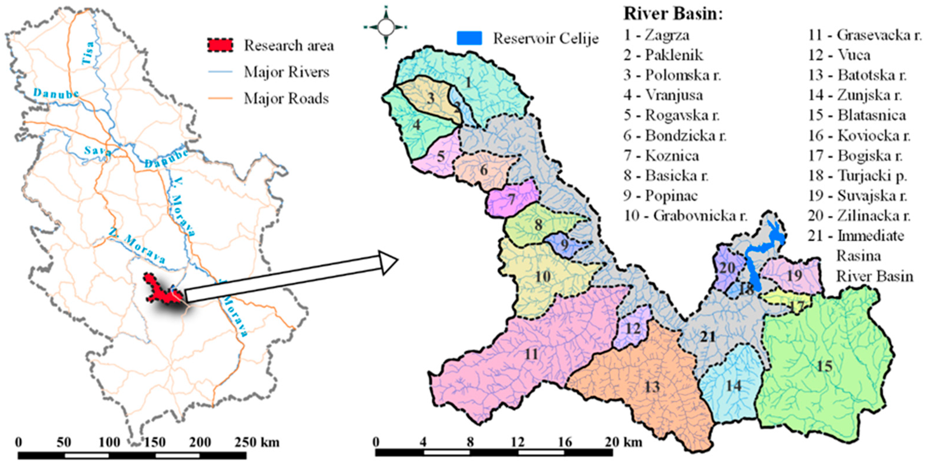
Figure 2.
(a) Slope map; (b) Hypsometric map of the Study area.
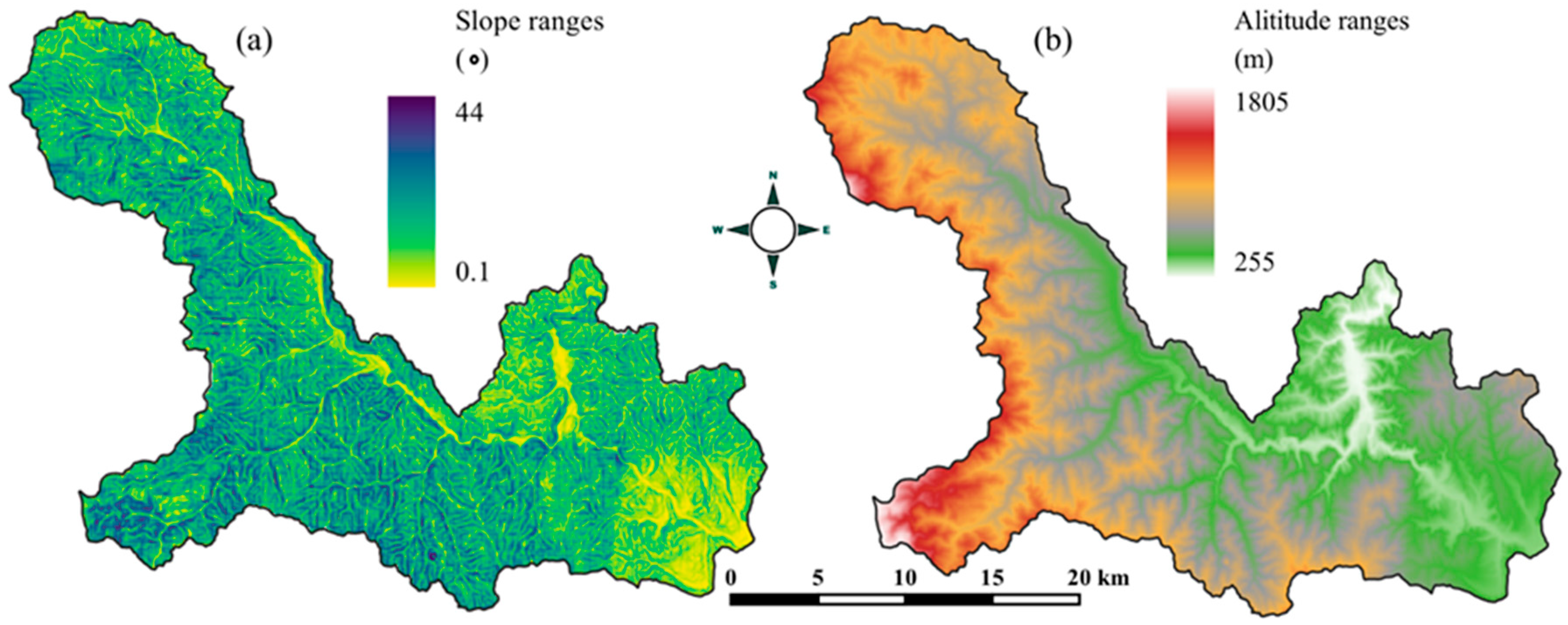
Figure 3.
(a) Soil map; (b) Map of the rock resistance to erosion.
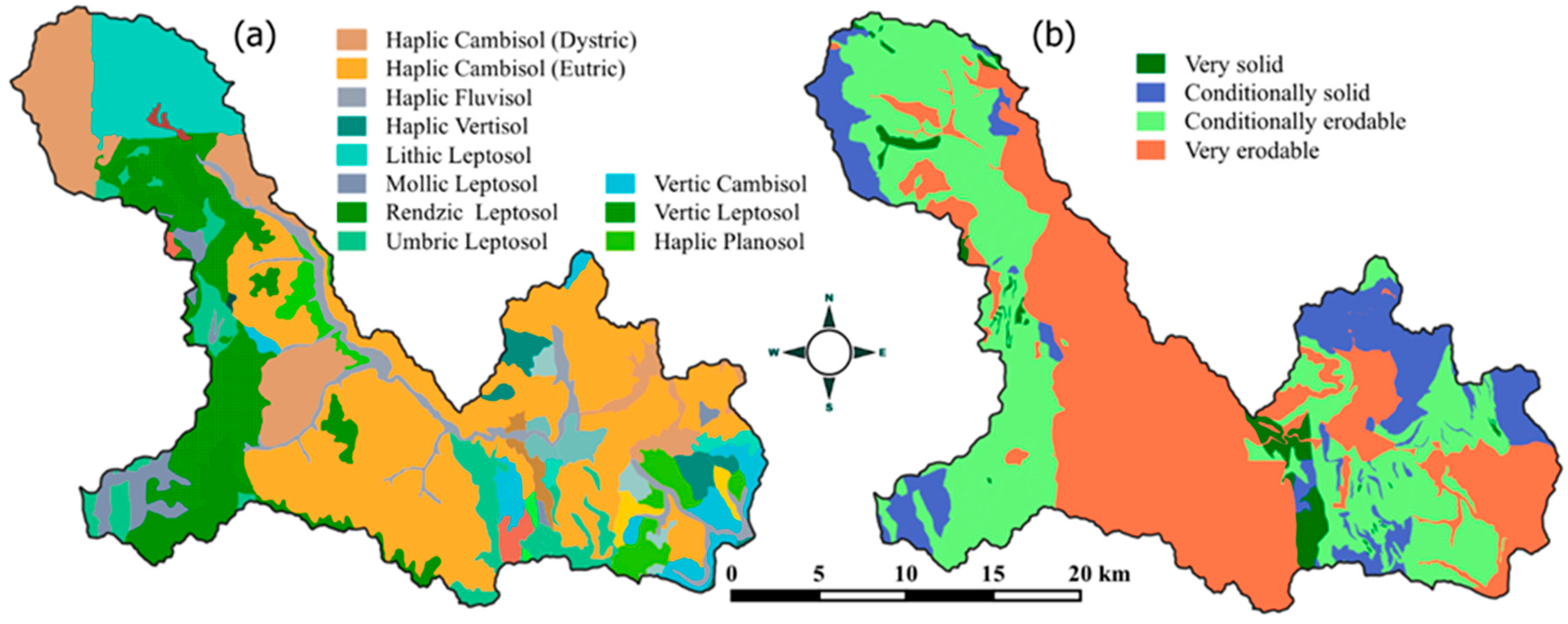
Figure 4.
(a) Isohyet map; (b) Isotherms map.
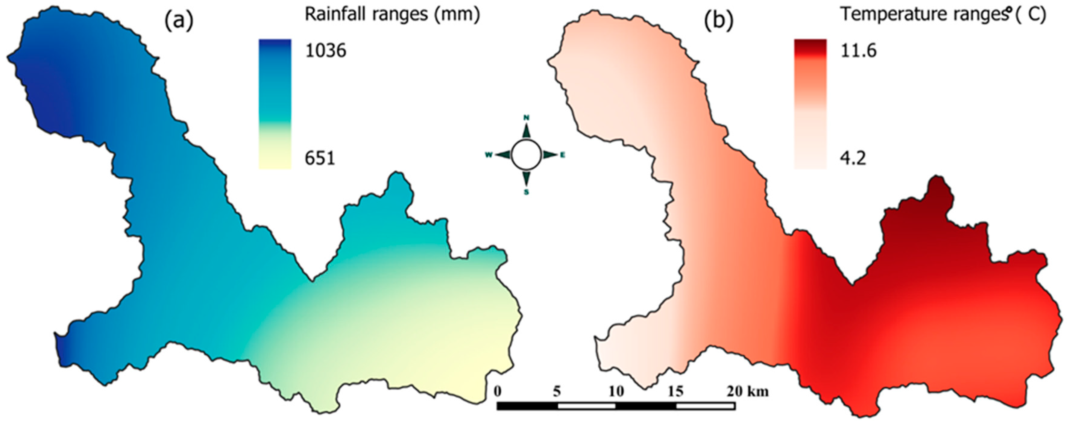
Figure 5.
Comparative review of number of population.
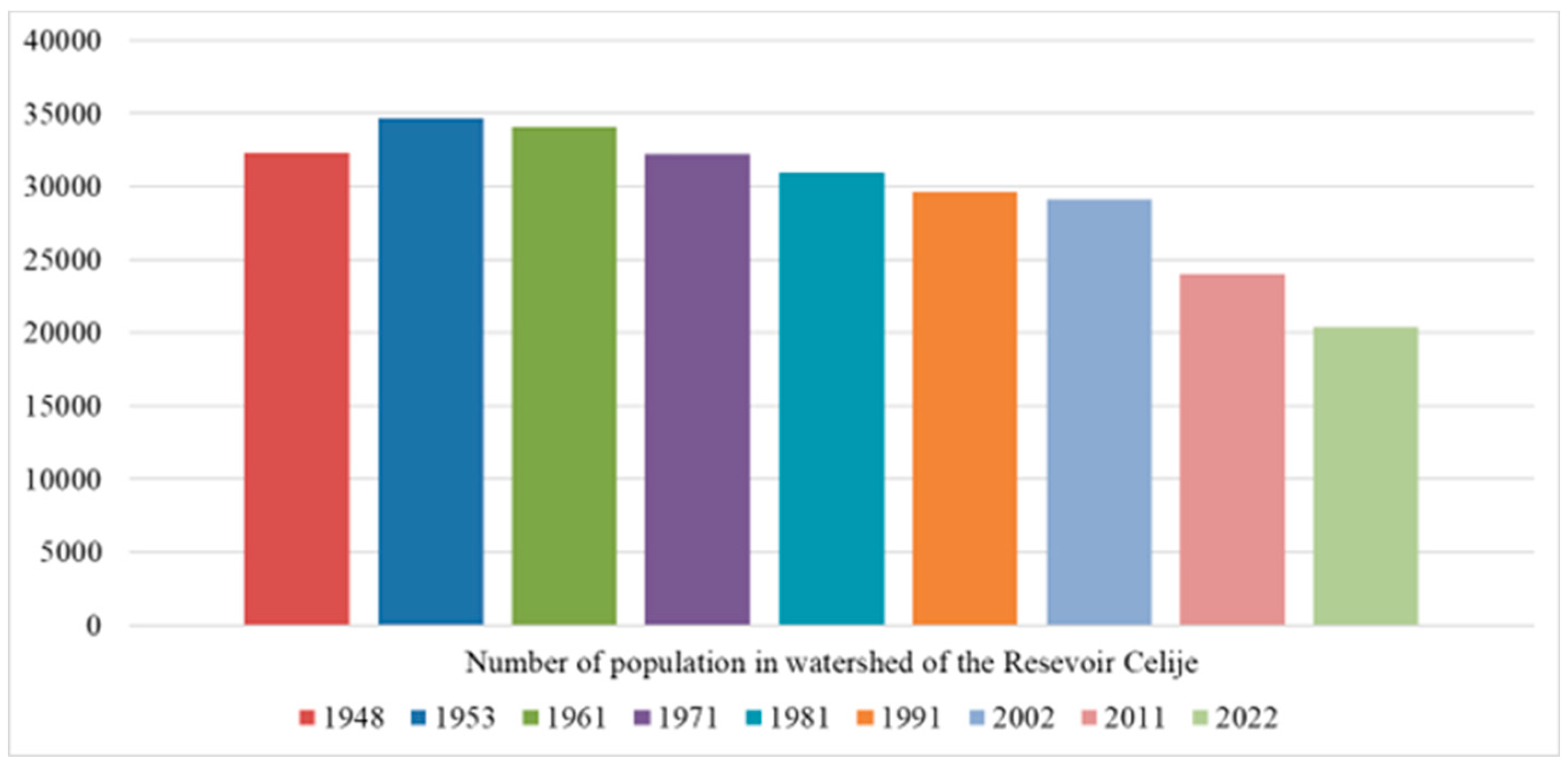
Figure 6.
Hydrographic map with existing check dams.
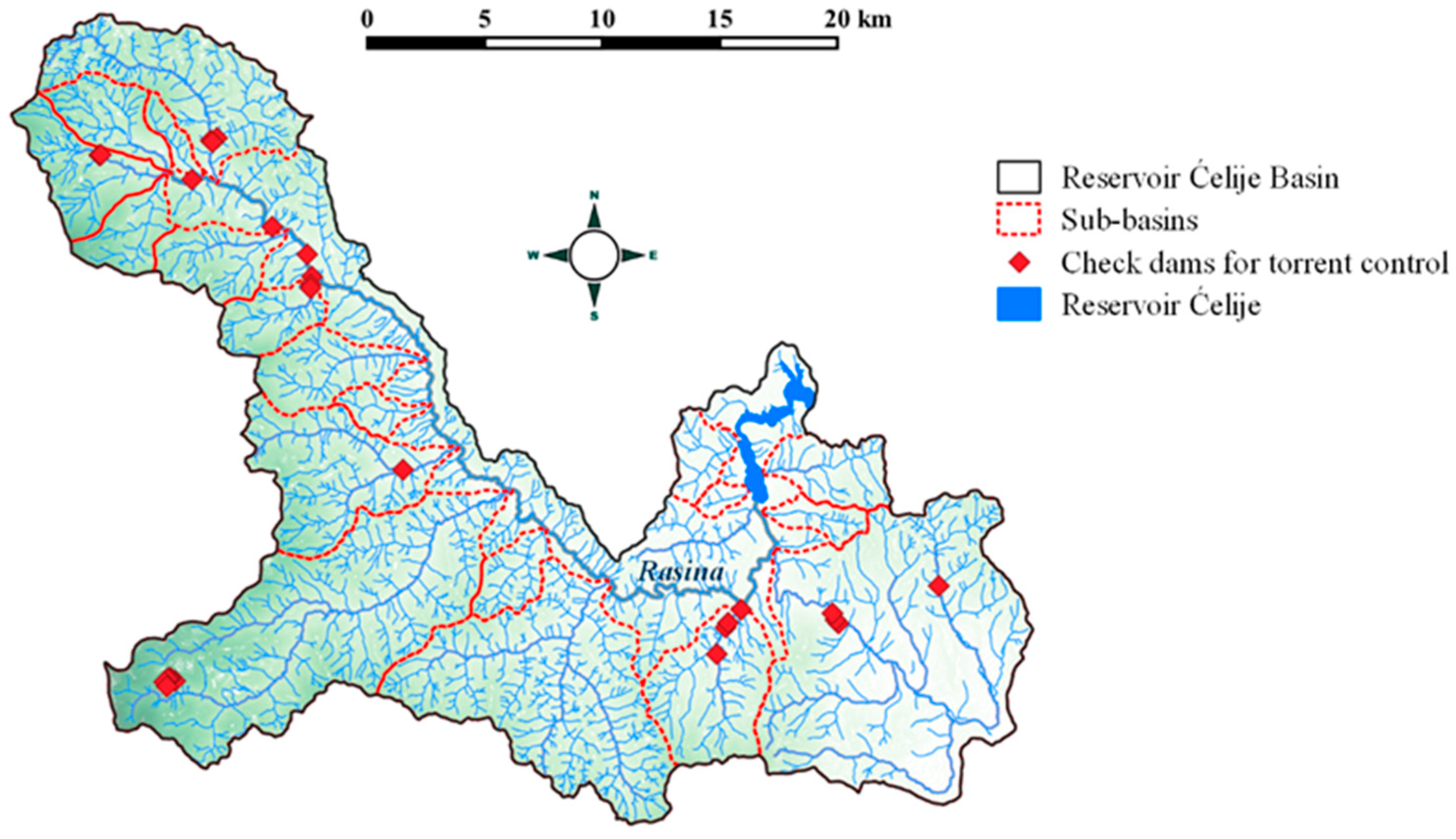
Figure 7.
Afforestation in watershed of Zunjska river: (a) 1968 (photo Z.Gavrilovic); (b) 2022 (photo I. Stefanovic).
Figure 7.
Afforestation in watershed of Zunjska river: (a) 1968 (photo Z.Gavrilovic); (b) 2022 (photo I. Stefanovic).
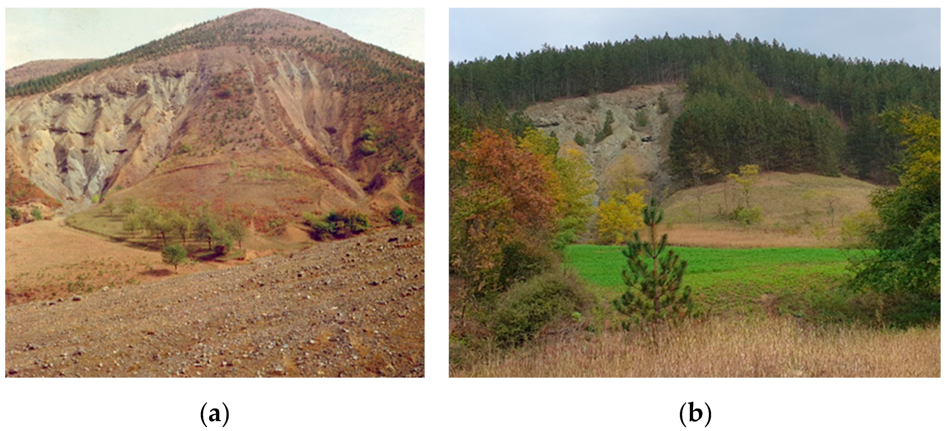
Figure 8.
Land use map: (a) 1968; (b) 2022.
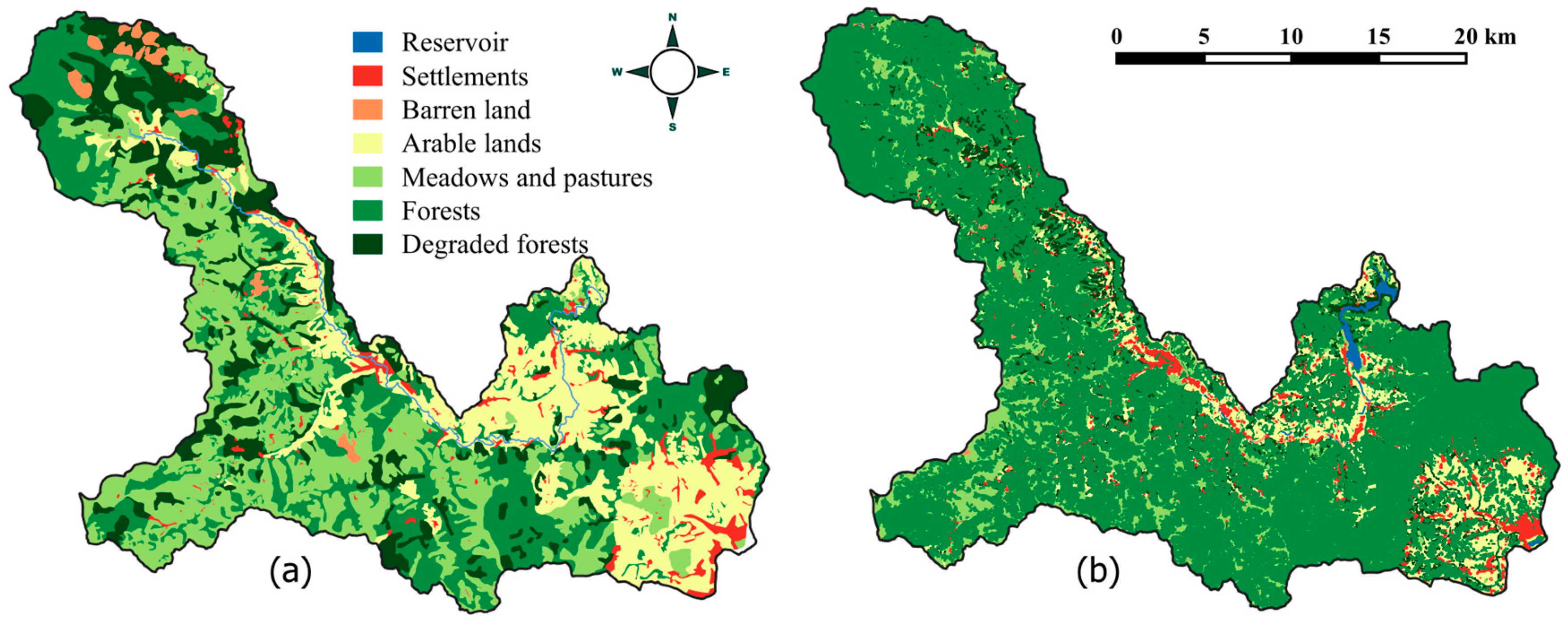
Figure 9.
Soil erosion map: (a) 1968; (b) 2022.
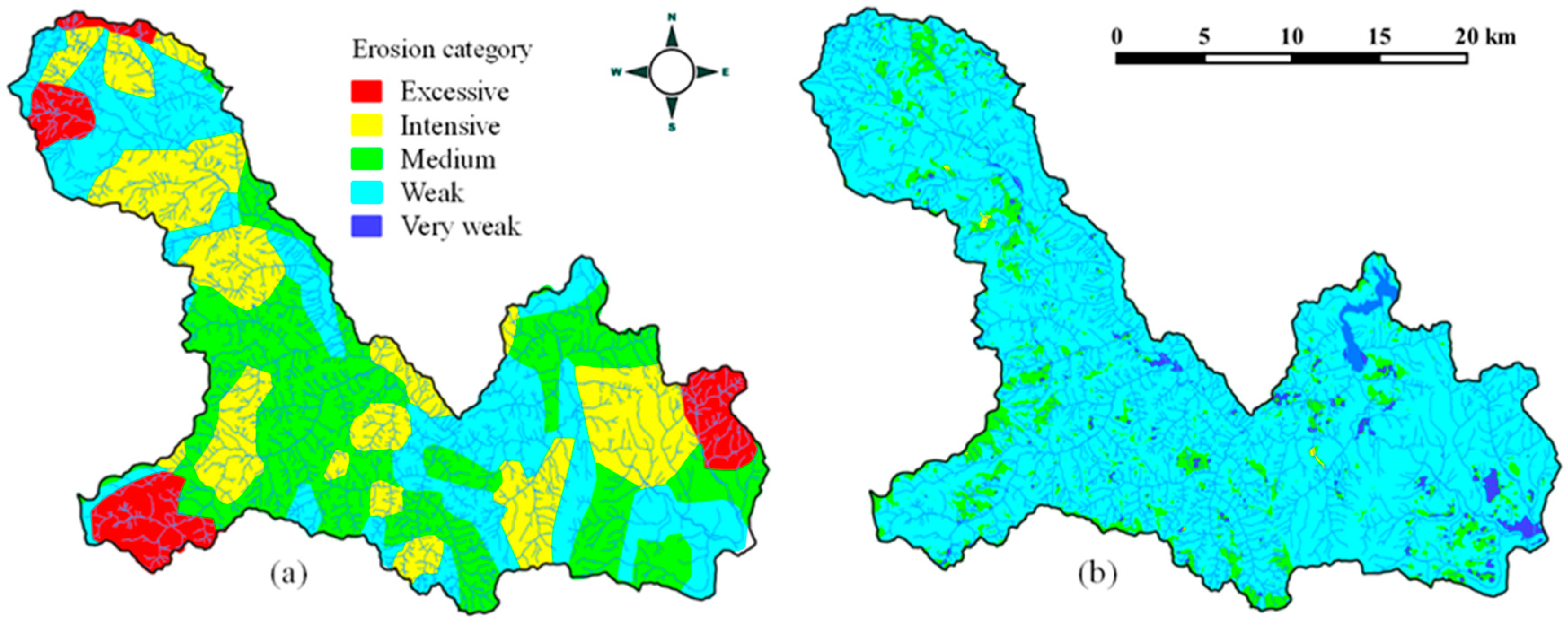
Figure 10.
Pearson`s correlation coefficient between slope of siltation (Iz) and natural bed slope (It).
Figure 10.
Pearson`s correlation coefficient between slope of siltation (Iz) and natural bed slope (It).
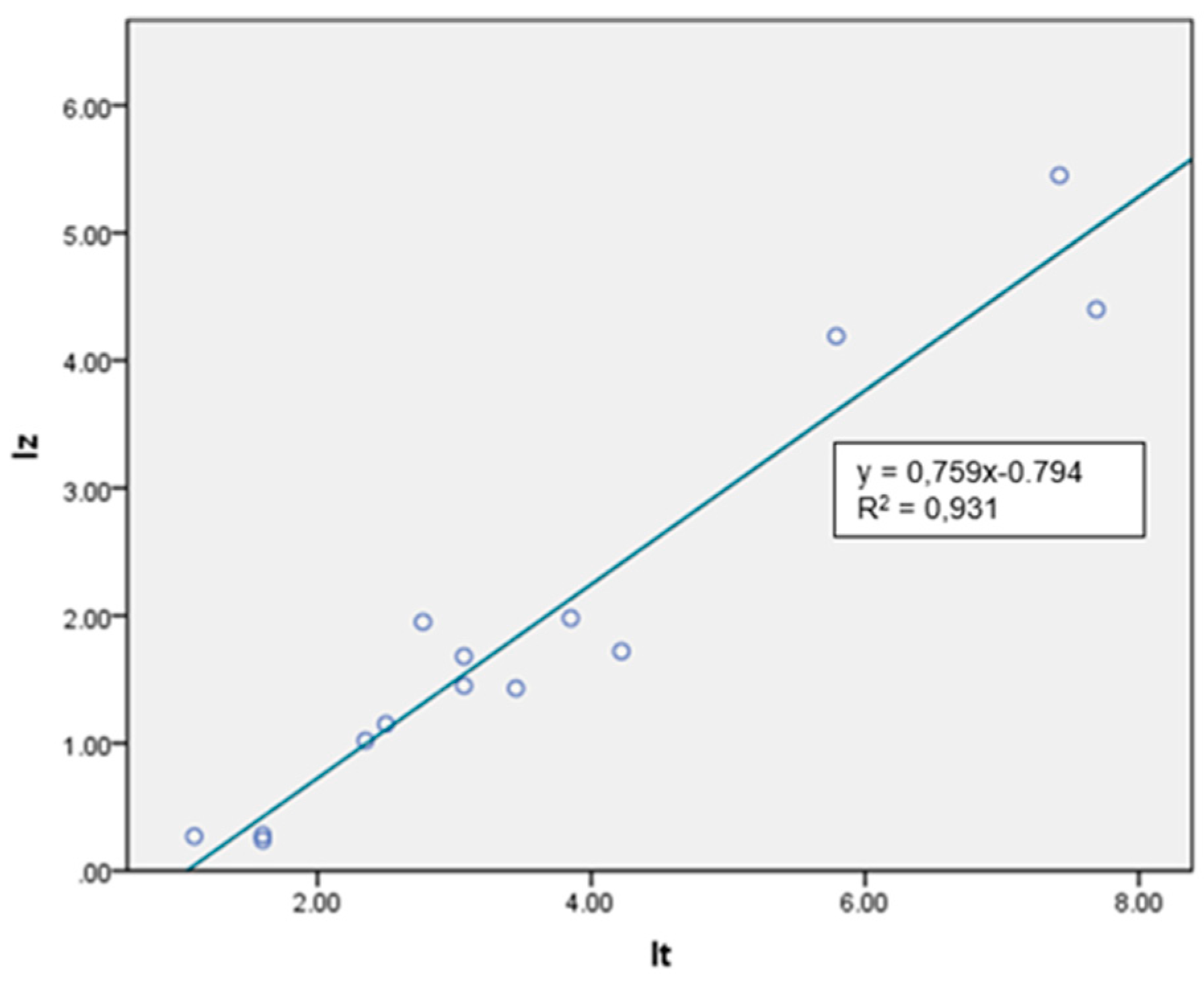

Table 1.
Physical characteristics of the Resevoir Celije watershed.
| Parameter | Mark | Value | Unit |
|---|---|---|---|
| Watershed area | А | 609,15 | km2 |
| Perimeter | О | 184,47 | km |
| River lenght | L | 69,95 | km |
| Watershed lenght | Ls | 49,39 | km |
| Peak point of the watershed | Hmax | 1936 | m |
| Confluence point of the watershed | Hmin | 239 | m |
| Mean slope of the riverbed | Iu | 1,62 | % |
| Mean slope of terrain | Isr | 34,65 | % |
| Mean altitude | Hsr | 695 | m |
| Mean altitude difference | D | 447 | m |
Table 2.
Meteorological stations in the Celije reservoir watershed.
| Meteorologicalstations | Coordinates | Elevation | Averageannualtemperature | Average annual rainfall | |
|---|---|---|---|---|---|
| X | Y | ||||
| m a.s.l. | °C | mm | |||
| Kruševac | 7528274.36 | 4824754.19 | 166 | 12.4 | 738 |
| Brus | 7502705.92 | 4804323.12 | 426 | 10.6 | 822 |
| Blace | 7524339.64 | 4795099.41 | 425 | 10.6 | 651 |
| Goč | 7487890.04 | 4822849.21 | 990 | 8.3 | 978 |
| Kopaonik | 7484294.00 | 4793337.00 | 1710 | 4.2 | 1035 |
| Jastrebac | 7528303.00 | 4814539.00 | 256 | 11.6 | 884 |
Table 3.
Basic characteristics of X, Y and φ coefficients used in EPM.
| Additional info | X description - soil protection | X |
| Before implementation ofanti-erosion measures | Completely bare, uncultivable land (bare land) | 1.00 |
| Arable land with plowing up or down hill | 1.00 | |
| Orchards and vineyards, without ground vegetation | 0.70 | |
| Mountain pastures and drylands | 0.60 | |
| Meadows, fields and similar agricultural crops | 0.40 | |
| Degraded forests and thickets with eroded soil | 0.60 | |
| Forests and thickets with good structure and vegetation | 0.05 | |
| After implementation ofanti-erosion measures | Plows with contour plowing (isohypsis direction) | 0.60 |
| Arable land well cared for and protected by mulching | 0.50 | |
| Contour strip cultivation with crop rotation (fields) | 0.45 | |
| Contour orchards and vineyards | 0.30 | |
| Terracing of arable land, terraces and tiers | 0.35 | |
| Weeding of bare land and melioration of pastures and drylands | 0.30 | |
| Construction of contour trenches of medium density | ||
| Retardation waterways and micro-accumulations | 0.25 | |
| Afforestation with construction of tiers | 0.10 | |
| Channel regulation, dam construction and channelization | 0.70 | |
| Y description - Soil erodibility | Y | |
| Sand, gravel and loose soils | 2.00 | |
| Loess, tuffs, salt marshes, steppe soils | 1.60 | |
| Disintegrated limestones and marls | 1.20 | |
| Serpentines, red sandstones, flysch deposits | 1.10 | |
| Podzol soils and alike; decomposed shales: micaschist, gneiss slates, clay slates | 1.00 | |
| Core limestones and shales, red rocks and humus-silicate soils | 0.90 | |
| Cambisol and mountain lands | 0.80 | |
| Vertisol, humogley and wetlands | 0.60 | |
| Chernozem and alluvial soils of good structure | 0.50 | |
| Bare compact eruptives (vulcanic origin) | 0.25 | |
| φ description - type and extent of erosion and slumps | φ | |
| Watershed completely under gully erosion and primordial processes | 1.00 | |
| About 80 % of the watershed is under furrow and gully erosion | 0.90 | |
| About 50 % of the watershed is under furrow and gully erosion | 0.80 | |
| The entire watershed is subject to surface erosion | 0.70 | |
| The entire watershed is under surface erosion, without deep processes | 0.60 | |
| Land with 50 % of the area covered by surface erosion | 0.50 | |
| Land with 20 % of the area covered by surface erosion | 0.30 | |
| No visible signs of erosion, minor slips and slides in watercourses | 0.20 | |
Table 4.
Classification of erosion coefficient Z and specific annual gross erosion W.
| Erosion Category | Erosion Intensity | Range of Z | Range of W (m3/km-2/year-1) |
|---|---|---|---|
| I | Excessive Erosion | 1.01-1.50 | >3000 |
| II | Intensive Erosion | 0.71-1.00 | 1200-3000 |
| III | Medium Erosion | 0.41-0.70 | 800-1200 |
| IV | Weak Erosion | 0.21-0.40 | 400-800 |
| V | Very Weak Erosion | 0.01-0.020 | 100-400 |
Table 5.
The Main Check dams effects.
| River Basin | No | It | Iz | Iz/It | hk | m | W | |
|---|---|---|---|---|---|---|---|---|
| % | % | m | m | m3 | ||||
| 1 | Blatasnica River | 1 | 1.6 | 0.28 | 0.18 | 4.0 | 19.5 | 11818.18 |
| 2 | 2 | 1.6 | 0.24 | 0.15 | 3.0 | 25.0 | 8272.06 | |
| 3 | 3 | 1.1 | 0.27 | 0.25 | 2.5 | 28.0 | 10542.17 | |
| 4 | Popovacka River | 1 | 3.45 | 1.43 | 0.41 | 1.5 | 14.5 | 807.55 |
| 5 | Zunjska River | 1 | 2.77 | 1.95 | 0.70 | 2.0 | 47.0 | 11463.41 |
| 6 | 2 | 3.07 | 1.68 | 0.55 | 3.0 | 35.0 | 11330.94 | |
| 7 | 3 | 3.07 | 1.45 | 0.47 | 3.0 | 22.0 | 6111.11 | |
| 8 | 4 | 4.22 | 1.72 | 0.41 | 5.0 | 44.0 | 22000.00 | |
| 9 | Koznicka River | 1 | 5.79 | 4.19 | 0.72 | 4.0 | 48.0 | 24000.00 |
| 10 | 2 | 7.69 | 4.40 | 0.57 | 5.5 | 19.0 | 8734.80 | |
| 11 | 3 | 7.42 | 5.45 | 0.73 | 3.0 | 22.0 | 5025.38 | |
| 12 | Zagrza | 1 | 2.35 | 1.02 | 0.43 | 3.0 | 14.0 | 4736.84 |
| 13 | 2 | 2.50 | 1.15 | 0.46 | 3.5 | 15.0 | 6805.56 | |
| 14 | Rasina River | 1 | 3.85 | 1.98 | 0.51 | 2.5 | 21.5 | 3592.91 |
Table 6.
Land Use in Watershed of the Reservoir Celije in 1968 and 2022.
| Year | 1968 | 2022 | ||
|---|---|---|---|---|
| Land Use | Areakm2 | % | Areakm2 | % |
| Forests | 201.35 | 33.05 | 384.19 | 63.07 |
| Barren land | 6.15 | 1.01 | 1.88 | 0.31 |
| Degraded forests | 97.25 | 15.96 | 54.55 | 8.96 |
| Meadows and pastures | 163.45 | 26.84 | 66.80 | 10.97 |
| Arable lands | 115.27 | 18.92 | 83.96 | 13.78 |
| Settlements | 25.68 | 4.22 | 14.53 | 2.38 |
| Reservoir | - | - | 3.25 | 0.53 |
| Total | 609.15 | 100 | 609.15 | 100 |
Table 7.
Surface areas according to the intensity of soil erosion in 1968 and 2022.
| Year | 1968 | 2022 | ||
|---|---|---|---|---|
| Erosion Category | Area km2 | % | Area km2 | % |
| Excessive Erosion | 54.74 | 8.99 | 0.03 | 0.00 |
| Intensive Erosion | 173.96 | 28.56 | 3.26 | 0.54 |
| Medium Erosion | 191.4 | 31.42 | 145.09 | 23.82 |
| Weak Erosion | 189.05 | 31.04 | 418.27 | 68.66 |
| Very Weak Erosion | - | - | 42.50 | 6.98 |
| Total | 609.15 | 100 | 609.15 | 100 |
Table 8.
Specific annual gross erosion and sediment transport.
| Specific annual gross erosion | Specific sediment transport | ||
|---|---|---|---|
| m3/ km-2 / year-1 | m3/ km-2 / year-1 | ||
| 1968 | 2022 | 1968 | 2022 |
| 1189.12 | 554.20 | 540.18 | 253.55 |
Table 9.
Total annual gross erosion and sediment transport.
| Total annual gross erosion | Total sediment transport | ||
|---|---|---|---|
| m3/ year | m3/ year | ||
| 1968 | 2022 | 1968 | 2022 |
| 724351.84 | 337589.51 | 329052.69 | 154450.81 |
Disclaimer/Publisher’s Note: The statements, opinions and data contained in all publications are solely those of the individual author(s) and contributor(s) and not of MDPI and/or the editor(s). MDPI and/or the editor(s) disclaim responsibility for any injury to people or property resulting from any ideas, methods, instructions or products referred to in the content. |
© 2024 by the authors. Licensee MDPI, Basel, Switzerland. This article is an open access article distributed under the terms and conditions of the Creative Commons Attribution (CC BY) license (http://creativecommons.org/licenses/by/4.0/).
Copyright: This open access article is published under a Creative Commons CC BY 4.0 license, which permit the free download, distribution, and reuse, provided that the author and preprint are cited in any reuse.