

Submitted:
02 February 2024
Posted:
02 February 2024
You are already at the latest version
Abstract
In this paper, we use a machine learning method, known as Nonnegative Matrix Factorization, to extract from a given image some new information obtained from a number of color space representations. Such kind of information, termed ``metacolor'', can be considered as a particular color space representation of the image, which can be used to obtain a binary segmentation of the investigated image by distinguishing foreground and background pixels. Some numerical experiments prove that the proposed method shows improved results when compared with common simpler thresholding algorithms.
Keywords:
Color Spaces
; Low Rank Data Representation
; Feature Extraction
; Machine Learning algorithm
; Nonnegative Matrix Facorization
; Image Segmentation
1. Introduction
Several techniques can be applied to locate in images distinct areas or objects, on the basis of the analysis of some image characteristics (such as pixel intensity values). Generally, the image background refers to parts of the image which cannot be counted, such as sky, water bodies, and other similar elements. Foreground objects, on the other hand, are represented by the identifiable items that can be isolated from each other. A binary segmentation process aims at distinguishing between foreground objects and background, and its realization paves the way to subsequent image processing tasks.
In this paper, we exploit a well-established machine learning technique, i.e. an unsupervised learning method known as Nonnegative Matrix Factorization (NMF), to extract features from a color image to provide an alternative color space representation. These features, termed “metacolors”, form an automatically selected color model of the given image that can be successfully used to perform image processing tasks, such as binary segmentation.
NMF can be applied to provide a low-rank approximation of a given nonnegative data matrix , by extracting meaningful nonnegative patterns, that are the columns of the factor , and the encoding coefficients, that are rows of the factor (with , being r generally user-defined), in such a way that . Since early works [1,2], where several images representing human faces were decomposed into parts-based representations roughly corresponding to items intelligible by human intuition (noses, mouths, eyes, etc.), NMF has been broadly used in many successful applications, including blind source separation, document clustering, object recognition, hyperspectral image analysis [3,4]. In the context of image processing, NMF demonstrated its usefulness in several tasks: identifying regions or objects into images [5]; improving the representation of positive local data (such as color histograms) [6]; encoding color channels for face recognition task [7]; processing three color channels simultaneously for generating new basis of images [8]. In [9], a numerical method based on NMF was proposed to integrate histograms of different color spaces characterizing a given image to improve the results coming from Otsu’s segmentation.
Moving from the basic idea proposed in [9], this paper illustrates a method which starts from the integration of different color channels into a structured representation, to extract a new color space representation of the investigated image by means of NMF. This new representation encodes image properties, namely metacolors, which aggregate the expression of multiple color characteristics of an image into a more compact form while allowing an interpretation in terms of basis vectors for the latent color space representation of the image.
2. Background and basic concepts
In the following sections, we review some basic concepts useful to describe the proposed method. We describe some color spaces commonly used to parameterize color images, as well as the concept of thresholding to segment images into two classes. Then NMF is introduced as a mechanism to integrate different color space representations of a given image I and to extract the metacolor space representation. Such an extracted information provide a compact representation of I and is used to segment I.
2.1. Color spaces
A color space can be defined as a mathematical model that illustrates how colors can be represented. Generally, it is a geometric three-dimensional representation of colors that assigns three numerical values to each distinct color channel. Various color spaces have been introduced in the literature to define specific attributes of color image pixels. Based on their definition, we can identify some categories of color spaces: fundamental, derived, and application-specific. A comprehensive review and evaluation of color spaces is reported in [10]. The RGB color space is the most frequently used: it codifies the channels R (red), G (green), and B (blue), often called primary colors, that are combined to represent color as it is perceived by human perception [11]. Linearly or nonlinearly transformations of the RGB space generate other color spaces. Figure 1 provides a classification of color spaces into (i) the primary spaces (based on the trichromatic theory and representing any color by combining the right amounts of the three primary colors), (ii) the luminance-chrominance spaces (in which one component represents the luminance and two others the chrominances), (iii) the perceptual spaces (that quantify the color perception using intensity, hue, and saturation), and (iv) the independent axis spaces (providing as less correlated components as possible in some statistical sense) [10,12,13,14].
In this work, the following color spaces are considered to represent a color image I.
- RGB is a color space based on the trichromatic theory [15] that relies on the idea that all colors can be represented using different shades of the three primary colors R (red), G (green), and B (blue). RGB is an additive color space realized through a 24-bit implementation (8 bit for each primary color channel, allowing for values ranging from 0 to 255). It is a real color space, in the sense that the primary colors can actually be physically generated in some light spectrum, and gives rise to any primary space via matrix linear transformations on color space components (particularly, additive or subtractive linear models can be used).
- CIE XYZ is a color space defined by CIE (International Commission on Illumination) [16]. The XYZ system adopts “imaginary” primaries X, Y, and Z that cannot be realized by actual color stimuli: they may be intended as derived parameters from the R, G, and B colors. space is related by the linear transformation with and, for convenience, the Y primary value is defined so that it corresponds to luminance.
- is a luminance-chrominance space that codifies the luminance and chrominance information of colors. It was developed as part of the Recommendation ITU-R BT.601 for worldwide digital component video standard and used in television transmissions. The color component Y is the luma or luminance specifying the perceived brightness of color, while the chrominance components and are color difference channels and represent the difference between the blue B and red R channels and a reference value Y, respectively [12]. As a result, and provide the hue and saturation information of the color. This color space is widely used by most of the state-of-the-art compression algorithms, in video systems, printing presses, and other art items since it better describes the range of colors and contrast.
- HSV is a perceptual space quantifying subjective human color perception using: brightness/intensity, which characterizes the luminous level of a color stimulus (how dark or luminous an area appears); hue, which measures how much an area appears to be similar to one of the main primary colors (red, green, blue, and yellow); saturation, which allows estimating an area colorfulness in relation to its brightness (it represents the purity of a perceived color). Particularly, H represents a given hue (chromatic content), S the saturation value (the ratio of chromatic and achromatic contents), and V the brightness value of a color pixel. is obtained by RGB using a nonlinear transformation, particularly the cylindrical-coordinate transformation.
It should be noted that any color space can be (variously) reduced to a one-dimensional gray-scale representation, namely a vector of gray intensity values, by applying some transformation to the original values of the color channels. Obviously, such a reduction, while simplifying the overall image processing, implies also a loss in the amount of information embedded in the original color image.
2.2. Overview of automatic thresholding segmentation
Image thresholding is the most basic technique for segmenting images: a binary segmentation can be obtained by simply assigning each pixel to a class by comparing its color intensity with a threshold value [17]. The basic idea in thresholding is that homogeneous areas inside an image correspond to a class of pixels possessing comparable color characteristics. Color histograms illustrate the distribution of colors in an image and can be used to detect the classes of pixels and to define a threshold useful to segment the original image.
Image thresholding methods can be characterized as bi-level or multilevel thresholding methods. Bi-level thresholding algorithms set a single threshold so that a binary image can be obtained, separating foreground from background pixels according to how closely they relate to the threshold value. These mechanisms generally produce appreciable results when there is a considerable variation in the pixel values between the two target classes; the threshold value can be maintained constant in low-noise images or adapted dynamically when noisy images are considered. If the image is more complex and contains various objects, multilevel thresholding methods can be used: a number of thresholds are considered to differentiate the pixel-related information, thus obtaining a multiclass segmentation of the image.
In general, image thresholding techniques are based on the construction of color histograms related to each color channel: each component of the color space can be segmented using a histogram, then the results are combined to produce a final segmentation. Due to the three-dimensional nature of color information, defining a color image’s histogram and selecting a threshold within this histogram can be challenging [18]. Gray-level image segmentation is implemented analogously by considering the histogram realized on the single gray channel.
In the following section, we briefly overview some of the simplest and most popular non-parametric histogram-based global thresholding techniques. These will be used in the experimental section to derive binary segmentation of a target [19,19].
In the following, we are going to briefly introduce some popular non-parametric histogram-based global thresholding techniques oriented to define a binary segmentation (i.e., a bi-level thresholding is applied). Such techniques will be adopted in the numerical experiments discussed later on. To provide a formal illustration of the thresholding techniques, a suitable scenario is formalized as follows.
Let be an image with pixels, and let h be the L-bin histogram illustrating the distribution of pixel intensities in a selected color channel, that is
where is the number of the image pixels at color level i, and L is the number of distinct levels (e.g., if 8-bit gray-scale image representation is considered, then ).
A histogram threshold k should be set to define two classes and including the pixels whose intensity is less than k and those whose intensity ranges in , respectively (i.e., background and foreground regions). By adopting some simplifying assumptions [20], the histograms can be normalized and regarded as probability distribution, so that
is meant as the probability of occurrence of the color intensity level i (as previously asserted, is the total number of pixel of the image I). In this way, the probability distributions for and are defined as
Given these assumptions, the following methods can be applied to perform the binary segmentation of the image I.
Ridler and Calvard. This method consists in an iterative algorithm that starts with an initial guess threshold value that is used to initially split the image histogram into two portions. Generally, is set to the average color level of the overall image or the average color level of a subset of the pixels of the image (e.g., the four corners) that is most likely to contain only background pixels [21,22]. Starting from , the algorithm proceeds at each iteration as follows:
- Compute the set of pixels in I with intensity level below the threshold ;
- Compute the mean intensity value of the pixels included into ;
- Compute the set of pixels in I with intensity level above the threshold ;
- Compute the mean intensity value of the pixels included into ;
- Evaluate the new threshold value as ;
- Iterate steps 1-5 while is greater than a fixed tolerance value.
In the end, a final threshold is provided and it is used to produce a binary segmentation of the image I.
Otsu. This method aims at deriving an optimal threshold value that maximizes the separation between the two classes , . The basic idea is to minimize the intra-class variance defined as the weighted sum of the variances of the foreground and background regions. It is computed as
where and are variances of the two classes and the sum is weighted by the previously defined class probability distributions and .
The optimal threshold value is the one minimizing this intra-class variance. When 2 classes are involved minimizing the intra-class variance is equivalent to maximizing inter-class variance defined as
being and .
The main steps performed by the Otsu algorithm are:
- Calculate the pixel frequency distribution histogram of I and the probability distribution of each intensity level ;
- Normalize the histogram so that it sums to one, and calculate the and ;
- Calculate the cumulative mean and cumulative variance of pixel values;
- For each threshold value k calculate the inter-class variance;
- Find that maximizes the inter-class variance.
In the end, a final threshold is provided and it is used to produce a binary segmentation of the image I.
Kapur. The Kapur, Sahoo, and Wong (KSW) thresholding algorithm (also known as the Kapur entropy-based thresholding algorithm) finds the optimal threshold that provides the greatest amount of information or reduces uncertainty when separating the image into foreground and background [23]. The method uses information theory to search an optimal threshold k that maximizes the sum of the entropy of the two classes and while computing the probability distribution of the image pixel intensities. The method considers the foreground and background of an image as two different signal sources and computes an optimal threshold maximizing the sum of the two class entropy.
Let us assume that the image I is segmented by a threshold k, and let us consider the entropies and of the two classes and :
The main steps performed by Kapur algorithm are:
- Calculate the pixel frequency distribution histogram of I and the probability distribution of each intensity level , ;
- Normalize the histogram so that it sums to one, and calculate the cumulative sum and ;
- Calculate the overall entropy of the two classes, that is ;
- Find that maximizes .
In the end, a final threshold is provided and it is used to produce a binary segmentation of the image I.
Tsai. Tsai’s moment-preserving method [24] is based on the idea to consider an image as the blurred vision of an ideal binary image. In this method, the best threshold is selected in such a way that the first three moments of the image are preserved in the resultant binary image. Defined the k-th moment as
then the optimal threshold is chosen as
being , , and .
3. Integration for image color features via low-rank factorization
As known, an image I can be regarded as a matrix of pixels. The rows and the columns of the matrix indicate the position of each pixel in the image. The values of the pixels indicate the pixel intensity with respect to some specific color space. More precisely, each pixel incorporates three distinct values related to the channels of the color space: the single pixel intensity is a combination of the intensities in three channels.
The peculiar color-space representation of an image can influence the result of many image processing tasks, as for instance image segmentation and object recognition. Appropriate color spaces for representing I are usually selected by testing them one by one to determine which is the most convenient for a specific task.
When segmentation tasks are considered, no color space has proven to be more effective than the others. Thus, choosing the appropriate color space remains one of the most challenging aspects of segmenting color images. Rather than looking for the best representation of I, in this work, we propose to derive a new global representation of I by integrating different color image properties. Particularly, we integrate color channels representing I using the NMF method to extract latent features from different color space representations.
Let us consider a color image composed by pixels. We can build a derived matrix including the vectorization of the color intensity values of each pixel evaluated along the different color channels involved in the color spaces described in Section 2.1. In this way, we can write
In other words, constitutes an enlarged representation of I, including the basic RGB color information, together with the device-independent imaginary primaries components (deriving from the CIE XYZ color space), the luminance and the blue and red chromaticity components (deriving from the YCbCr color space), the intensity, hue, and luminosity information (deriving from the HSV color space), and the gray-scale channel component. Figure 2 illustrates an example image in its different color space representation.
Due to the nonnegative property of elements in , we can use the NMF algorithm [2,3] to extract new meta-features hidden into this enlarged representation of I. We indicate these meta-features as “metacolors” which can be regarded as the channels of a new color space offering an alternative representation of the image I.
3.1. Metacolors extraction from
NMF decomposes into an additive combination of a basis matrix and an encoding factor , both having non-negative elements, so that . The rank r is the tuning parameter in NMF; in this work, we set , to represent the usual dimension of the color spaces describing a color image I. The columns of W are the metacolors and they are an additive combination of color channels; they can be considered as an alternative color representation of the image pixels storing all the information of the image in the selected color spaces.
As concerning the computation of W and E from , the 2-block coordinate descent Alternating Nonnegative Least Square (ANLS) is used [3]. Starting from random nonnegative factors [25], this method approximates, in an alternate manner, the solution of the following two convex sub-problems connected with NMF factorization of :
and
The algorithm used the following update rules [26]:
where denotes the iteration step. Updates are performed until a stopping criterion (total number of iterations) is satisfied. Figure 3 illustrates the three metacolors obtained when the Bird example image is considered. Metacolors represent the basis of latent information embedded in different color representations of I. This additional knowledge can be used either to reconstruct I or, as we propose in this work, to undergo a binary segmentation step (which can be performed by any thresholding segmentation algorithm described in Section 2.2). Particularly, we used the metacolors as more informative features for enhancing the performance of thresholding segmentation methods. The main phases of the proposed NMF-based segmentation framework are sketched in Figure 4.
4. Numerical results and discussions
The proposed NMF-based method for thresholding segmentation has been evaluated both qualitatively and quantitatively. The qualitative evaluation was conducted on four benchmark color images (represented in Figure 5) by referring to an empirical goodness inspection simply based on human intuition [27]. The quantitative evaluation was conducted on a subset of 25 images randomly chosen from the PASCAL VOC2012 dataset (http://host.robots.ox.ac.uk/pascal/VOC/voc2012/index.html). This dataset includes color images of objects (airplanes, birds, cars, etc.) depicted into realistic scenarios (Figure 6 depicts two images of this dataset with their corresponding ground truth binary segmentation). The dataset also includes the corresponding ground truth binary segmentation of each image, therefore a numerical evaluation has been performed by adopting the following quantitative metrics:
- accuracy indicates the number of pixels classified correctly for a given class c,
- sensitivity it evaluates the proportion of pixels in the segmentation that correspond to boundary pixels in the ground truth (it corresponds to the precision);
- , F-measure provides the predictive performance of the binary threshold model;
- it provides a quick assessment of the segmentation performance;
- the Matthews correlation coefficient indicates the ineffectiveness of the binary segmentation in classifying pixels;
- ; it scores the overlap between predicted segmentation and ground truth, penalizing in highly class imbalanced images;
- Jaccard index measures the similarity between the predicted segmentation and its ground truth image segmentation;
- specitivity evaluates the capabilities for correctly identifying pixels in the background;
The above formalizations assume that, for a given class , is the number of pixels classified correctly as c; is the number of pixels classified incorrectly as c; is the number of pixels classified correctly as not c, and the number of pixels classified incorrectly as not c.
All the experiments are conducted on the same PC with 1.6 GHz Intel Core i5 dual-core, 16-GB memory, and without external GPU; the segmentation algorithms and the NMF-based approach were run in MATLAB R2023b.
For the sake of comparison, in Figure 7, Figure 8, Figure 9 and Figure 10(a) we report the results of the segmentation obtained by applying the thresholding algorithms used as reference methods (i.e., Otsu, Kapur, Tsai, Ridler) to the benchmark images involved in the qualitative evaluation. The illustrated results relate to the segmentation obtained by referring to the gray-scale image representation. Analogously, in Figure 7, Figure 8, Figure 9 and Figure 10(b) we report the segmentation results obtained by applying the same thresholding algorithms to the benchmark images represented in terms of the novel metacolor space defined through the proposed NMF-based method (as described in Figure 4). As it can be observed, the reference thresholding algorithms are able to identify the main objects in the foreground of the image with a few inaccuracies. Such inaccuracies are somewhat corrected by the application of the NMF-based segmentation. In fact, a better distinction between glasses and shadows can be observed for the Martini glasses image (Figure 7), and the foreground objects appear to be well-separated from the background. When we turn to consider the starfish image (Figure 8) the improvement of the results is more appreciable in a better background identification. The Airplane object (Figure 9) is better identified, providing a more clear appearance of the silhouette of the object in flight. In the Table image (Figure 10) the proposed method allows a better identification of the actual form of the object (especially when Otsu and Ridler algorithms are considered).
Concerning the quantitative analysis, Table 1 reports the average values of the previously introduced metrics resulting from the segmentation processes performed over the 25 images collected from the PASCAL VOC12 dataset. As can be seen, the values related to the application of the proposed method are comparable with the performance exhibited by the classical thresholding algorithms applied to the gray-scale images, and in some cases they indicate an improvement in the segmentation quality deriving from the extraction of the metacolor space. This is specially true when Otsu and Kapur algorithms are considered, thus confirming an enhanced discriminating ability.
5. Conclusion
In this paper, we addressed the problem of binary segmentation of color images, that is discriminating pixels into the classes: background to foreground. Information related to various color channels, represented by color spaces, are integrated using an NMF algorithm and metacolors are extracted to represent hidden knowledge that can be used to improve the segmentation process. Particularly, given a color image I to segment, it is firstly represented using different color channels (four color spaces are used each of them having three color features). This information is then integrated into a new data matrix embedding features extracted each original color feature. This enlarged image matrix representation is mined using Nonnegative Matrix Factorization algorithm to extract metacolors on which a thresholding algorithm is applied to segment the original image and give the final segmented binary image.
The proposed NMF-based approach provides improved binary segmentation results compared with standard algorithm on gray-scale image representation and appears to better identify background pixels. Future developments will include the detection of various objects in color image, rather than just concentrating on the foreground and background, the interpretation of metacolors in terms of image characteristics.
Author Contributions
“All the authors contribute equally to the Conceptualization, writing—original draft preparation, software and validation, writing—review and editing this work. All authors have read and agreed to the published version of the manuscript.’
Funding
This research received no external funding.
Data Availability Statement
Codes and Image used in this paper are available, numerical codes are available on request
Acknowledgments
This work was supported in part by the GNCS-INDAM (Gruppo Nazionale per il Calcolo Scientifico of Istituto Nazionale di Alta Matematica) Francesco Severi, P.le Aldo Moro, Roma, Italy.
Conflicts of Interest
The authors declare no conflicts of interest.
References
- Lee, D.D.; Seung, H.S. Learning the parts of objects by non-negative matrix factorization. Nature 1999, 401, 788–791. [Google Scholar] [CrossRef] [PubMed]
- Lee, D.D.; Seung, H.S. Algorithms for Non-negative Matrix Factorization. Proc Adv Neur Inf Proc Sys. MIT Press, 2000, Vol. 13, pp. 556 – 562.
- Gillis, N. Nonnegative Matrix Factorization; SIAM, 2020.
- Yuan, Z.; Oja, E. Projective Nonnegative Matrix Factorization for Image Compression and Feature Extraction. Image Analysis; Kalviainen, H., Parkkinen, J., Kaarna, A., Eds.; Springer Berlin Heidelberg: Berlin, Heidelberg, 2005; pp. 333–342. [Google Scholar]
- Guillamet, D.; Schiele, B.; Vitria, J. Analyzing non-negative matrix factorization for image classification. 2002 International Conference on Pattern Recognition, 2002, Vol. 2, pp. 116–119 vol.2.
- Guillamet, D.; Vitria, J.; Schiele, B. Introducing a weighted non-negative matrix factorization for image classification. Pattern Recognition Letters 2003, 24, 2447–2454. [Google Scholar] [CrossRef]
- Rajapakse, M.; Tan, J.; Rajapakse, J. Color channel encoding with NMF for face recognition. 2004 International Conference on Image Processing, 2004. ICIP ’04., 2004, Vol. 3, pp. 2007–2010 Vol. 3.
- Luong, T.X.; Kim, B.K.; Lee, S.Y. Color image processing based on Nonnegative Matrix Factorization with Convolutional Neural Network. 2014 International Joint Conference on Neural Networks (IJCNN), 2014, pp. 2130–2135. [CrossRef]
- Castiello, C.; Del Buono, N.; Esposito, F. Improving Color Image Binary Segmentation Using Nonnegative Matrix Factorization. Computational Science and Its Applications – ICCSA 2023 Workshops; Gervasi, O., Murgante, B., Rocha, A.M.A.C., Garau, C., Scorza, F., Karaca, Y., Torre, C.M., Eds.; Springer Nature Switzerland: Cham, 2023; pp. 623–640. [Google Scholar]
- Kahu, S.Y.; Raut, R.B.; Bhurchandi, K.M. Review and evaluation of color spaces for image/video compression. Color Research and Applications 2018. [Google Scholar] [CrossRef]
- Gowda, S.N.; Yuan, C. ColorNet: Investigating the Importance of Color Spaces for Image Classification. Computer Vision – ACCV 2018; Jawahar, C., Li, H., Mori, G., Schindler, K., Eds.; Springer International Publishing: Cham, 2019; pp. 581–596. [Google Scholar] [CrossRef]
- Busin, L.; Shi, J.; Vandenbroucke, N.; Macaire, L. Color space selection for color image segmentation by spectral clustering. Proc. of IEEE Int Conf Sig Im Proc Appl - ICSIPA09, 2009, pp. 262–267. [CrossRef]
- Vandenbroucke, N.; Macaire, L.; Postaire, J.G. Color image segmentation by pixel classification in an adapted hybrid color space. Application to soccer image analysis. Comput Vis Image Underst 2003, 90, 190–216. [Google Scholar] [CrossRef]
- Ganesan, P.; Sathish, B.S.; Vasanth, K.; Sivakumar, V.G.; Vadivel, M.; Ravi, C.N. A Comprehensive Review of the Impact of Color Space on Image Segmentation. 2019 5th International Conference on Advanced Computing and Communication Systems (ICACCS), 2019, pp. 962–967. [CrossRef]
- Distante, A.; Distante, C. Color. In Handbook of Image Processing and Computer Vision: Volume 1: From Energy to Image; Springer International Publishing: Cham, 2020; pp. 79–176. [Google Scholar]
- Hugh, S. Fairman, Michael H. Brill, H.H. How the CIE 1931 color-matching functions were derived from Wright-Guild data. Color Research and Application 1998, 22, 11–23. [Google Scholar] [CrossRef]
- Linda, G. Shapiro (Autore), G.C.S. Computer Vision, 2001. [Google Scholar]
- Cheng, H.D.; Jiang, X.H.; Sun, Y.; Wang, J.L. Color image segmentation: Advances and prospects. Patt Recogn 2001, 34, 2259–2281. [Google Scholar] [CrossRef]
- Jain, S.; Laxmi, V. Color Image Segmentation Techniques: A Survey. 2018.
- Otsu, N. A Threshold Selection Method from Gray-Level Histograms. IEEE Transactions on Systems, Man, and Cybernetics 1979, 9, 62–66. [Google Scholar] [CrossRef]
- Ridler, T.W. .; Calvard, S. Picture Thresholding Using an Iterative Selection Method. IEEE Transactions on Systems, Man, and Cybernetics 1978, 8, 630–632. [Google Scholar] [CrossRef]
- Xue, J.H.; Zhang, Y.J. Ridler and Calvard’s, Kittler and Illingworth’s and Otsu’s methods for image thresholding. Pattern Recognition Letters 2012, 33, 793–797. [Google Scholar] [CrossRef]
- Kapur, J.; Sahoo, P.; Wong, A. A new method for gray-level picture thresholding using the entropy of the histogram. Computer Vision, Graphics, and Image Processing 1985, 29, 273–285. [Google Scholar] [CrossRef]
- Tsai, W.H. Moment-preserving thresolding: A new approach. Computer Vision, Graphics, and Image Processing 1985, 29, 377–393. [Google Scholar] [CrossRef]
- Esposito, F. A Review on Initialization Methods for Nonnegative Matrix Factorization: Towards Omics Data Experiments. Mathematics 2021, 9, 1006. [Google Scholar] [CrossRef]
- Berry, M.; Browne, M.; Langville, A.; Pauca, P.; Plemmons, R. Algorithms and Applications for Approximate Nonnegative Matrix Factorization. Computational Statistics and Data Analysis 2007, 52, 155–173. [Google Scholar] [CrossRef]
- Zhang, Y. A survey on evaluation methods for image segmentation. Patt Recog 1996, 29, 1335–1346. [Google Scholar] [CrossRef]
Figure 1.
A rough classification of color space based on its characteristics (a more complete illustration can be found in [14]).
Figure 1.
A rough classification of color space based on its characteristics (a more complete illustration can be found in [14]).
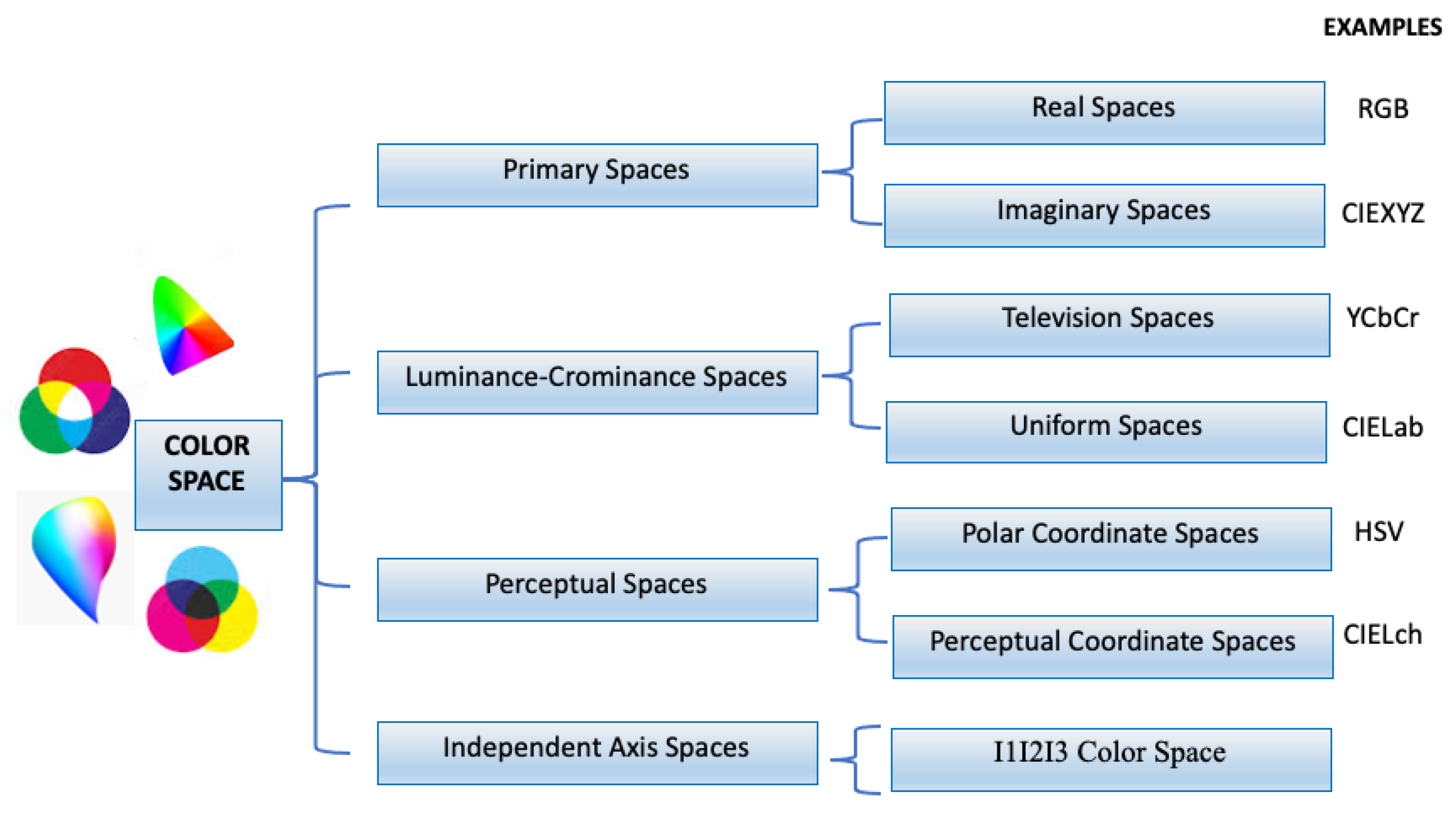
Figure 2.
Bird example image represented in the selected color spaces (from dataset PASCAL VOC2012 ID-image 2008_000123) (a-d) RBG image and the corresponding color channels R, G, and B; (e-h) CIExyz image and the corresponding color channels x, y, and z; (i-l) YCbCr image and the corresponding color channels Y, Cb, and Cr; (m-p) HVS image and the corresponding color channels H, V, and S.
Figure 2.
Bird example image represented in the selected color spaces (from dataset PASCAL VOC2012 ID-image 2008_000123) (a-d) RBG image and the corresponding color channels R, G, and B; (e-h) CIExyz image and the corresponding color channels x, y, and z; (i-l) YCbCr image and the corresponding color channels Y, Cb, and Cr; (m-p) HVS image and the corresponding color channels H, V, and S.
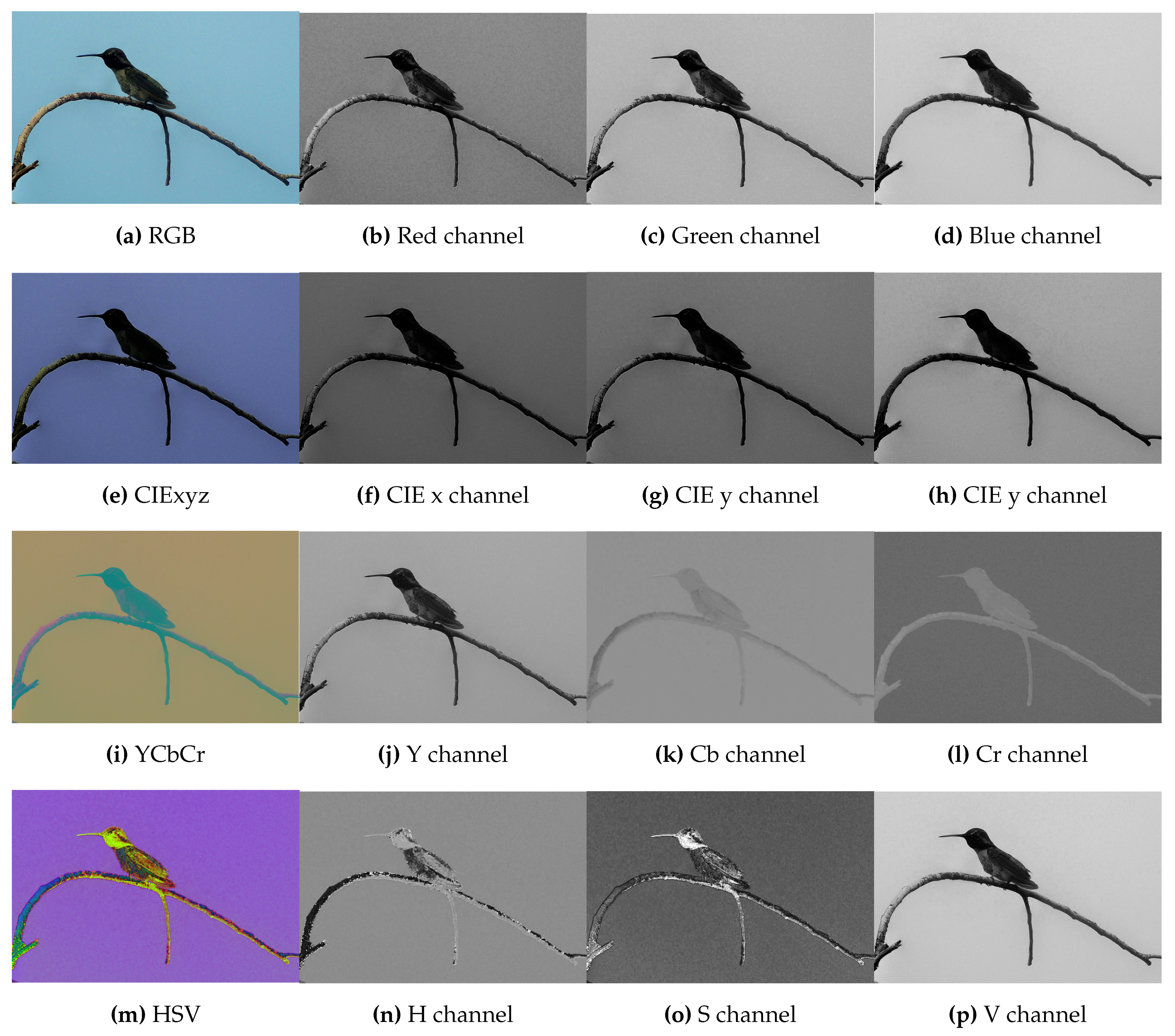
Figure 3.
Example of metacolors obtained factorizing the enlarged representation of the bird example image with rank value .
Figure 3.
Example of metacolors obtained factorizing the enlarged representation of the bird example image with rank value .
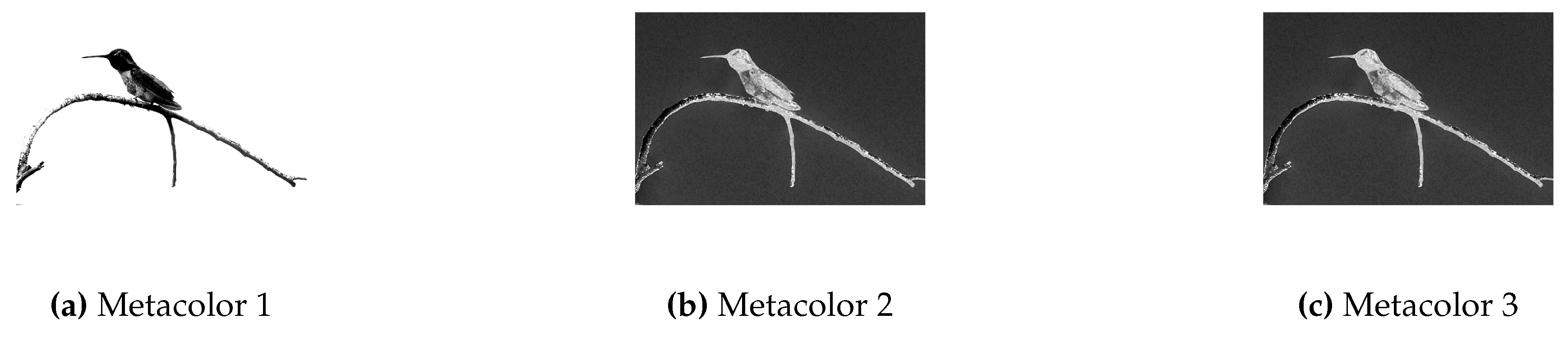
Figure 4.
Flowchart of NMF-based segmentation algorithm. The sequential phases of the proposed approach are: the construction of an enlarged representation of the input color image, feature integration, and meta-colors extraction, new image representation, and a final binary threshold segmentation step.
Figure 4.
Flowchart of NMF-based segmentation algorithm. The sequential phases of the proposed approach are: the construction of an enlarged representation of the input color image, feature integration, and meta-colors extraction, new image representation, and a final binary threshold segmentation step.
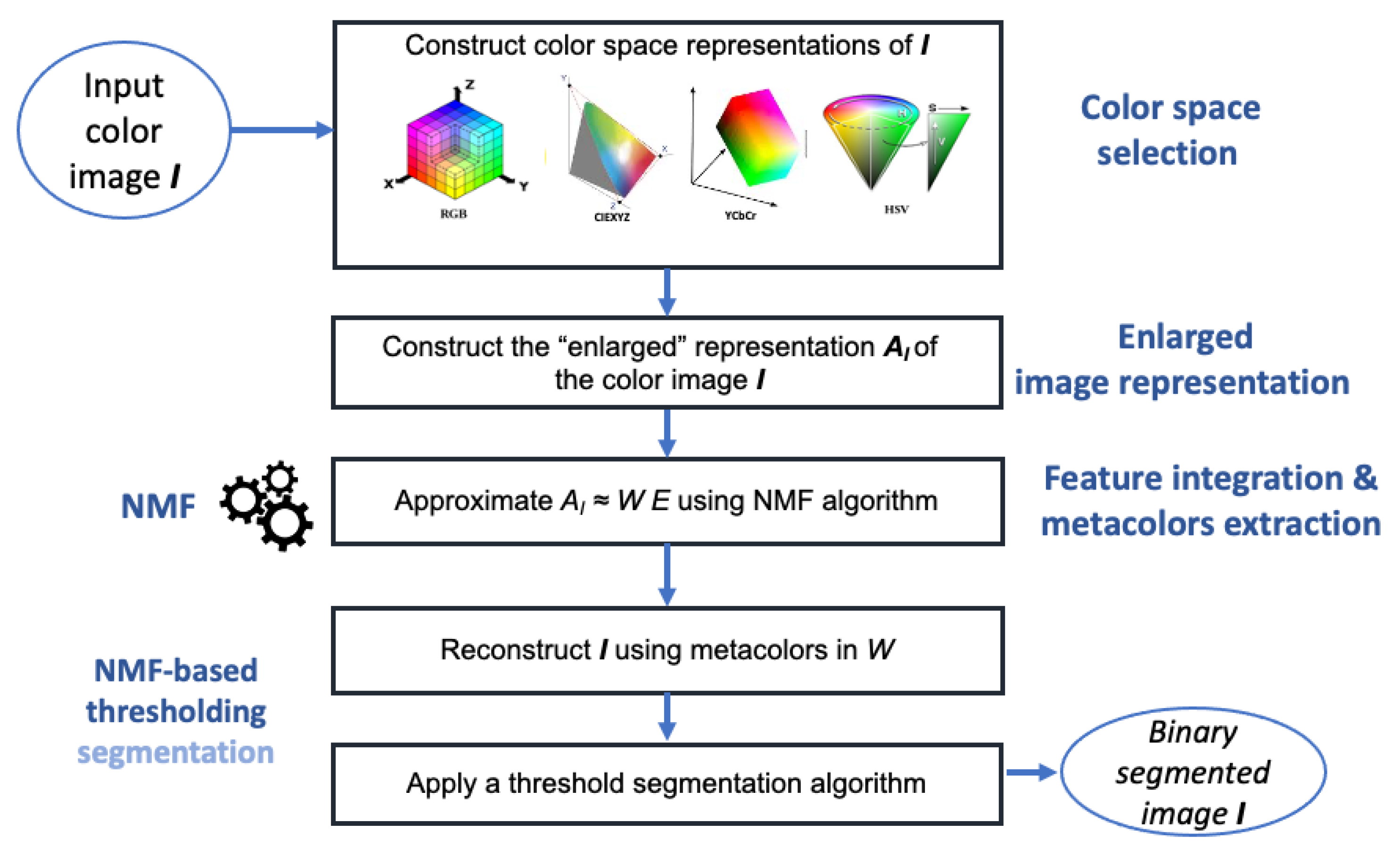
Figure 5.
Images used for the qualitative evaluation of the segmentation results obtained from the threshold segmentation algorithms.
Figure 5.
Images used for the qualitative evaluation of the segmentation results obtained from the threshold segmentation algorithms.
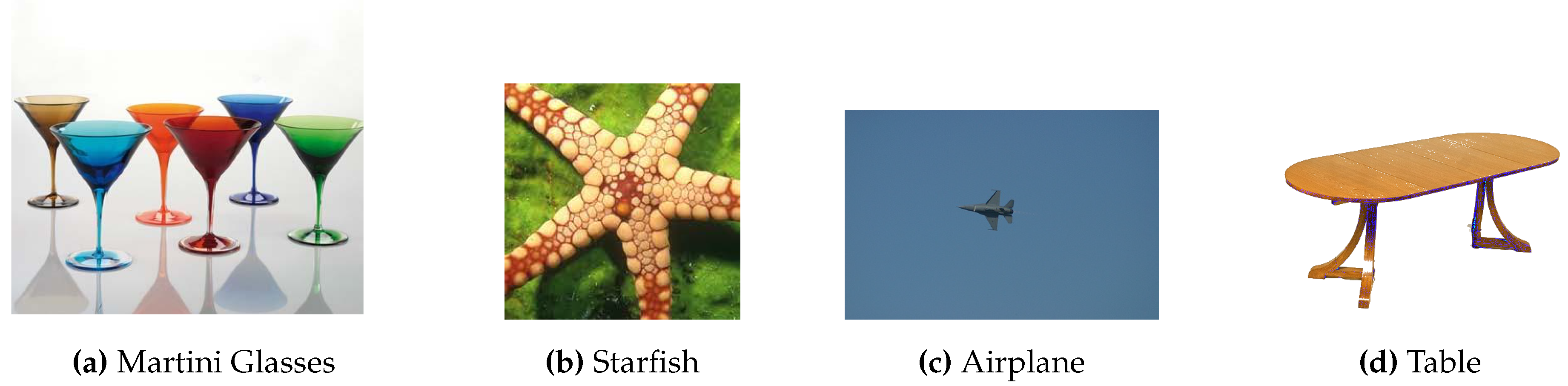
Figure 6.
Two images included in the dataset used for the quantative evaluation of the segmentation results obtained from the threshold segmentation algorithms and their corresponding ground truth.
Figure 6.
Two images included in the dataset used for the quantative evaluation of the segmentation results obtained from the threshold segmentation algorithms and their corresponding ground truth.
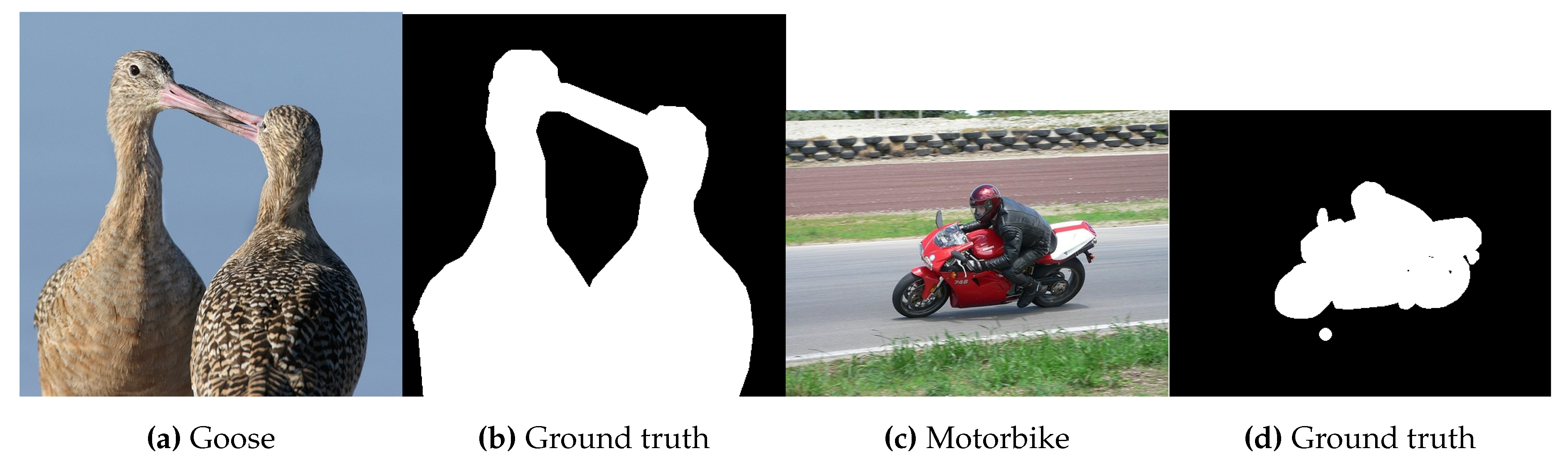
Figure 7.
Binary segmentation obtained using: (a) the threshold algorithms on the original image and (b) the NMF-based segmentation approach on the Martini Glasses image.
Figure 7.
Binary segmentation obtained using: (a) the threshold algorithms on the original image and (b) the NMF-based segmentation approach on the Martini Glasses image.
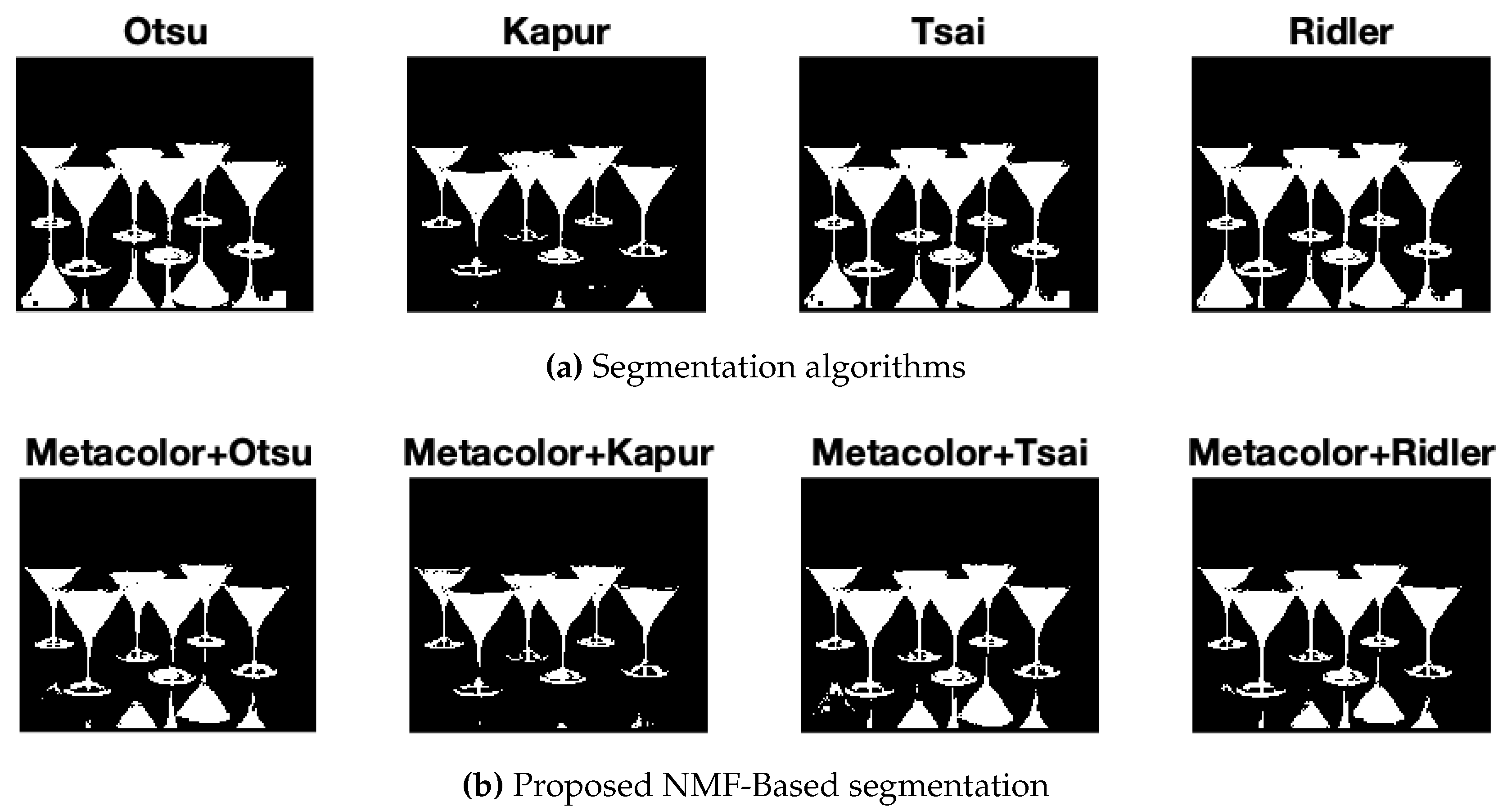
Figure 8.
Binary segmentation obtained using: (a) the threshold algorithms on the original image and (b) the NMF-based segmentation approach on the Starfish image.
Figure 8.
Binary segmentation obtained using: (a) the threshold algorithms on the original image and (b) the NMF-based segmentation approach on the Starfish image.
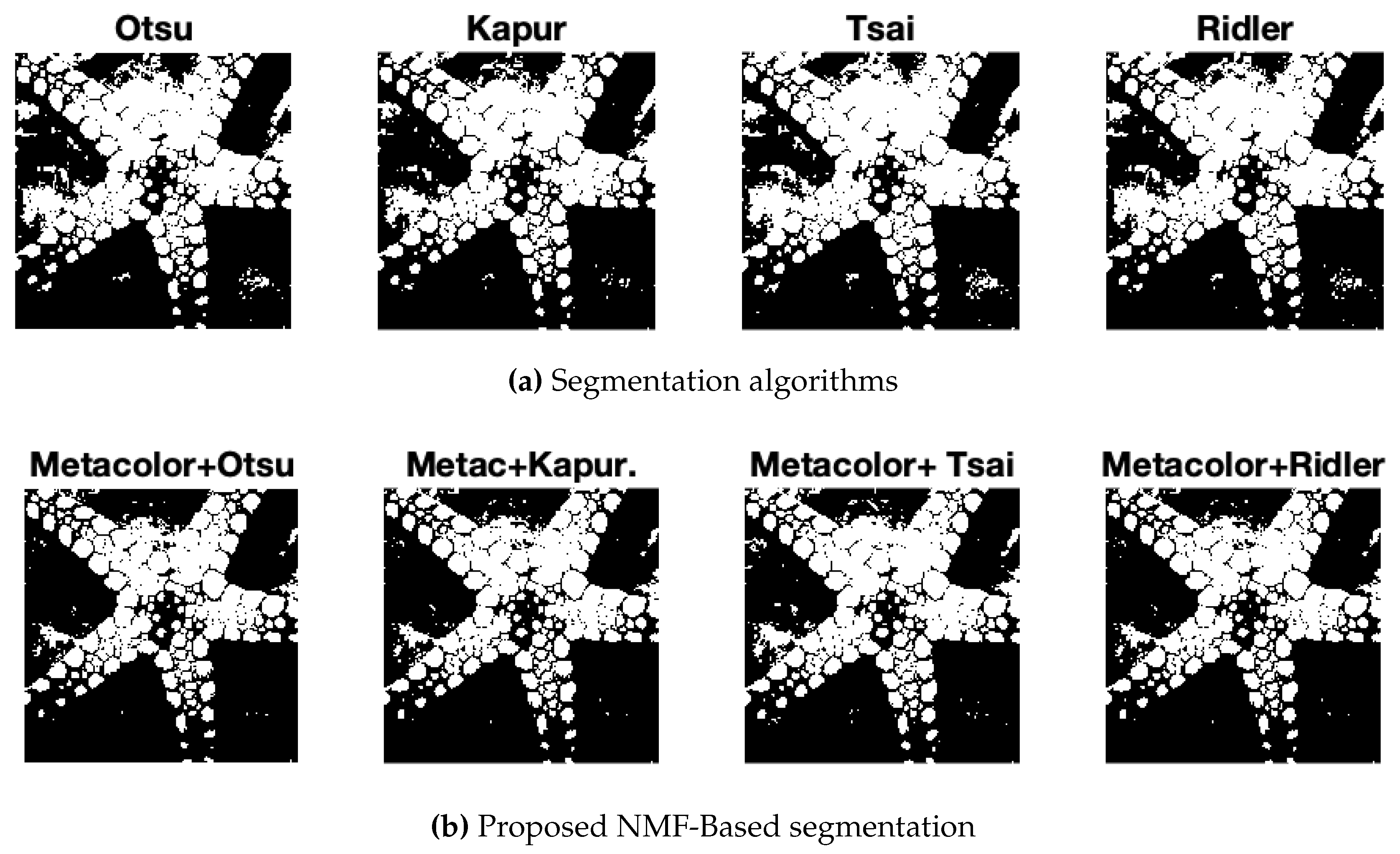
Figure 9.
Binary segmentation obtained using: (a) the threshold algorithms on the original image and (b) the NMF-based segmentation approach on the Airplane image.
Figure 9.
Binary segmentation obtained using: (a) the threshold algorithms on the original image and (b) the NMF-based segmentation approach on the Airplane image.
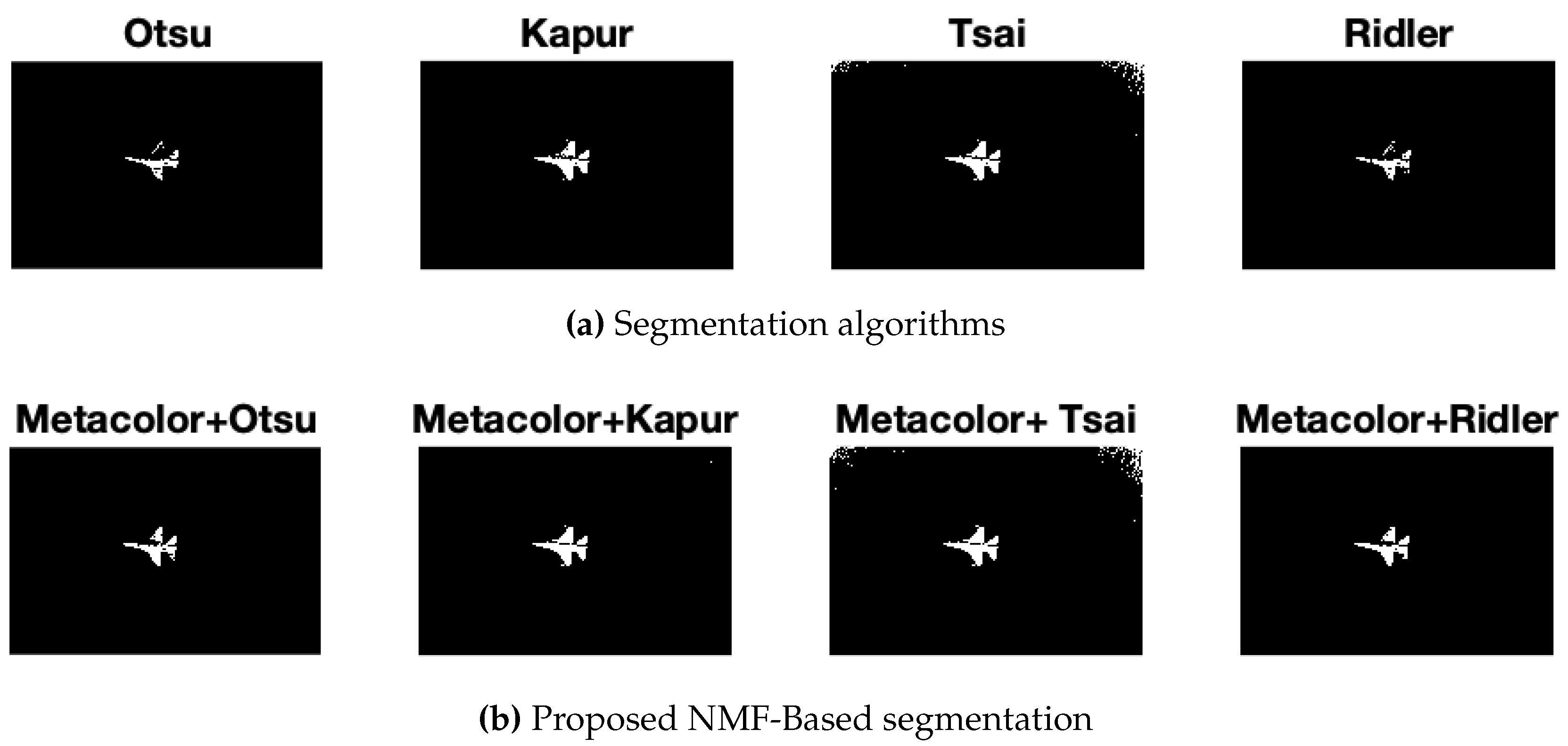
Figure 10.
Binary segmentation obtained using: (a) the threshold algorithms on the original image and (b) the NMF-based segmentation approach on the Table image.
Figure 10.
Binary segmentation obtained using: (a) the threshold algorithms on the original image and (b) the NMF-based segmentation approach on the Table image.
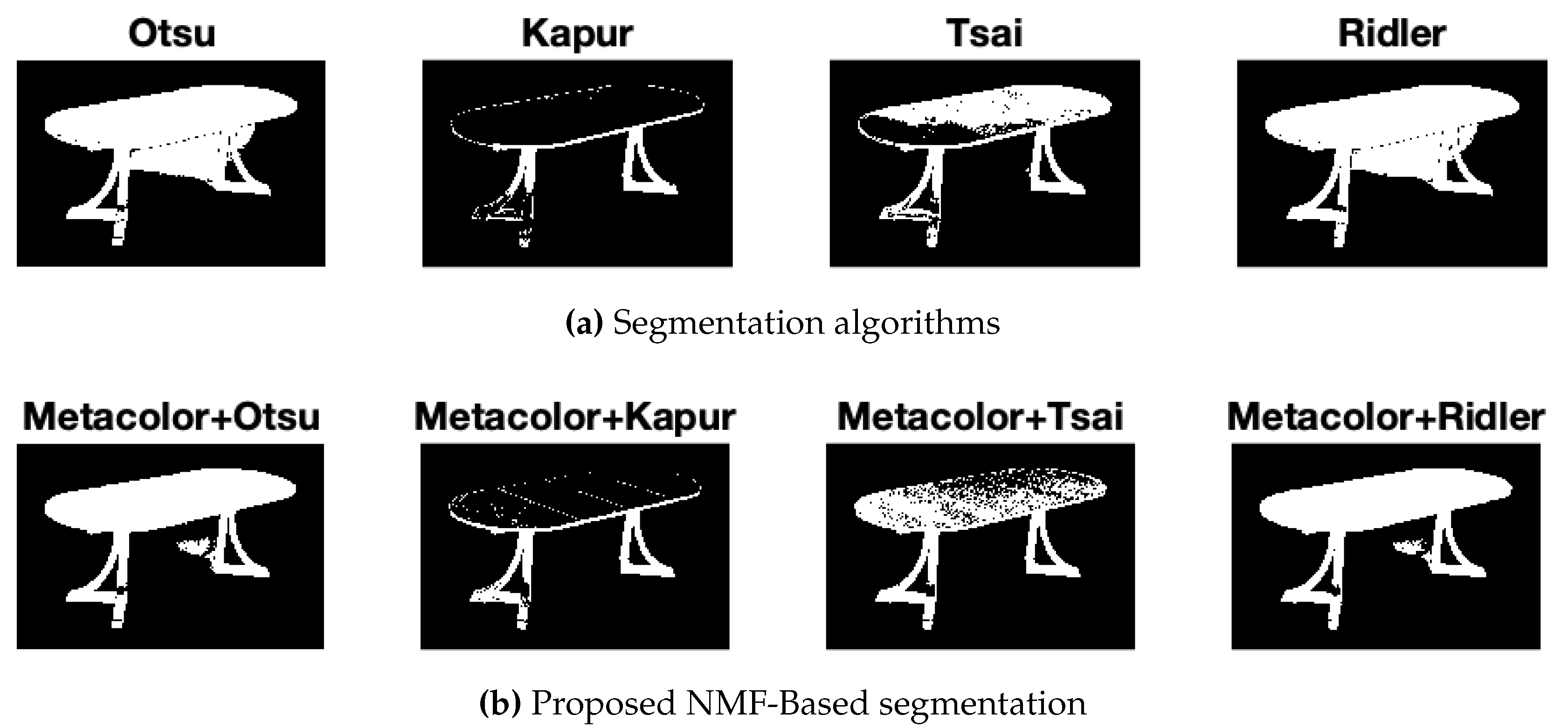

Table 1.
Mean and standard deviation for the quantitative measures used to evaluate segmentation results with respect to the known ground-truth on the all selected 25 images.
Table 1.
Mean and standard deviation for the quantitative measures used to evaluate segmentation results with respect to the known ground-truth on the all selected 25 images.
| Otsu | Metac+Otsu | Kapur | Metac+Kapur | Ridler | Metac+Ridler | Tsai | Metac+Tsai | |
| 0.7443 ± 0.1555 | 0.7455 ± 0.1667 | 0.6356 ± 0.2774 | 0.6812 ± 0.2434 | 0.7420 ± 0.1701 | 0.7466 ± 0.1420 | 0.7295 ± 0.1759 | 0.7284 ± 0.1241 | |
| 0.7484 ± 0.3011 | 0.7345 ± 0.3000 | 0.6568 ± 0.3411 | 0.6834 ± 0.3514 | 0.7340 ± 0.3002 | 0.7443 ± 0.3049 | 0.7311 ± 0.3021 | 0.7451 ± 0.2993 | |
| F | 0.6947 ± 0.2613 | 0.7118 ± 0.2585 | 0.6068 ± 0.3296 | 0.5593 ± 0.3539 | 0.7131 ± 0.2581 | 0.6945 ± 0.2636 | 0.6987 ± 0.2585 | 0.6763 ± 0.2606 |
| 0.6843 ± 0.2327 | 0.7308 ± 0.2102 | 0.6538 ± 0.3198 | 0.5289 ± 0.3579 | 0.7368 ± 0.2037 | 0.6921 ± 0.2253 | 0.7140 ± 0.2086 | 0.6575 ± 0.2386 | |
| 0.3945 ± 0.2978 | 0.3891 ± 0.3020 | 0.2323 ± 0.3780 | 0.2463 ± 0.3554 | 0.3895 ± 0.3035 | 0.3897 ± 0.3014 | 0.3701 ± 0.2953 | 0.3720 ± 0.2944 | |
| 0.6947 ± 0.2613 | 0.7118 ± 0.2585 | 0.6068 ± 0.3296 | 0.5993 ± 0.3539 | 0.7131 ± 0.2581 | 0.7145 ± 0.2636 | 0.6763 ± 0.2606 | 0.6987 ± 0.2585 | |
| 0.5865 ± 0.2873 | 0.6074 ± 0.2895 | 0.5088 ± 0.3277 | 0.4683 ± 0.3456 | 0.6088 ± 0.2888 | 0.5970 ± 0.2885 | 0.5905 ± 0.2858 | 0.5640 ± 0.2858 | |
| 0.6391 ± 0.2967 | 0.6551 ± 0.2970 | 0.5584 ± 0.3098 | 0.5654 ± 0.2935 | 0.6559 ± 0.2977 | 0.6790 ± 0.2955 | 0.6286 ± 0.2893 | 0.6240 ± 0.2965 |
Disclaimer/Publisher’s Note: The statements, opinions and data contained in all publications are solely those of the individual author(s) and contributor(s) and not of MDPI and/or the editor(s). MDPI and/or the editor(s) disclaim responsibility for any injury to people or property resulting from any ideas, methods, instructions or products referred to in the content. |
© 2024 by the authors. Licensee MDPI, Basel, Switzerland. This article is an open access article distributed under the terms and conditions of the Creative Commons Attribution (CC BY) license (http://creativecommons.org/licenses/by/4.0/).
Copyright: This open access article is published under a Creative Commons CC BY 4.0 license, which permit the free download, distribution, and reuse, provided that the author and preprint are cited in any reuse.


