Preprint
Article

A Theory of Everything: When Information Geometry Meets the Generalized Brownian Motion and the Einsteinian Relativity

Altmetrics

Downloads

157

Views

88

Comments

0

This version is not peer-reviewed

Submitted:

24 January 2024

Posted:

25 January 2024

You are already at the latest version

Alerts
Abstract
Information geometry (IG) is a fascinating combination of differential geometry and statistics where a Riemannian manifold's structure is applied to a statistical model. It may find numerous fascinating uses in the domains of theoretical neurology, machine learning, complexity, and (quantum) information theory, among others. (IG) aims to provide a differential-geometric perspective on statistical geodesic models' structure. In this case, IG, KD, and J-divergence (JD) are used to define the manifold of the Generalised Brownian Motion (GBM). Consequently, the geodesic equations (GEs) are devised, and GB information matrix exponential (IME) is presented. Moreover, for first time ever, the necessary and sufficient mathematical requirement that characterizes the developability of Generalized Brownian Motion(GBM) manifold is devised. Also, a novel sufficient and necessary conditions which characterizes the regions where the surface describing GBM is minimal is determined. Also, it is shown that GBM has a non-zero 0-Gaussian and Ricci curvatures. Consequently, this advances the establishment of a unified GBM- Relativistic Info-Geometric based analysis.
Keywords: 
Subject: Computer Science and Mathematics  -   Applied Mathematics

1. Introduction

1.1. Information Geometry

Stochastic control, neural networks, statistical inference, and other study domains have all made extensive use of information geometry (IG) [1].To put it another way, IG seeks to integrate statistics with differential geometry (DG) methods. Applying non-Euclidean geometry approaches and techniques to probability theories and stochastic processes is, thus, the central premise of IG. A topological finite dimensional Cartesian space, R n , where one possesses an infinite-dimensional manifold, is called a manifold [2-4]. The challenge of making decisions can be applied to the parameter inference θ ^   of a model based on data in Figure 1.
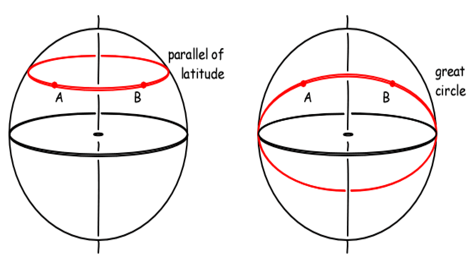
Matrix exponential plays a significant role in Lie groups theory [5,6]. From a visual perspective, Figure 2 portrays the geometric representation of geodesics on curved surfaces.
Einstein's theory of classical general relativity (GR) holds that objects travel along a geodesic in a curved space-time that extremizes the proper time between two locations. A geodesic, which reduces the distance between two places, is also known as a "straight line on a curved surface."

1.2. Generalized Brownian Motion (GBM)

Simple physical systems’ internal diffusion was firstly defined by Einstein [8-39].
The Tsallisian entropic measure in discrete domain reads:
H q = 1 q 1 ( 1 n = 1 ( p n ) q ) (1.1)
where p n is the probability of being in the n t h state. In the limit q 1 , the Tsallis entropy reduces to the Boltzmann-Gibbs entropy.
The Tsallisian entropic measure in continuous domain reads:[40-42]
H q X = 1 q 1 ( 1 f X x q   d x ) (1.2)
where f X x is PDF( X )
P D F q G a u s s i a n reads
f x = β C q e q ( β x 2 ) (1.3)
with
e q x = [ 1 + 1 q x ] 1 ( 1 q ) (1.4)
is called the q-exponential, C q is a normalization constant, and β > 0   is a scale parameter, and q , 1 < q < 3 finetunes extensivity, for a distributional similarity scaling β = ν + 1 2 ν = 1 3 q .

1.3. Random Diffusivity [41]

Looking at
d X t = ν d t + D d B ( t ) (1.5)
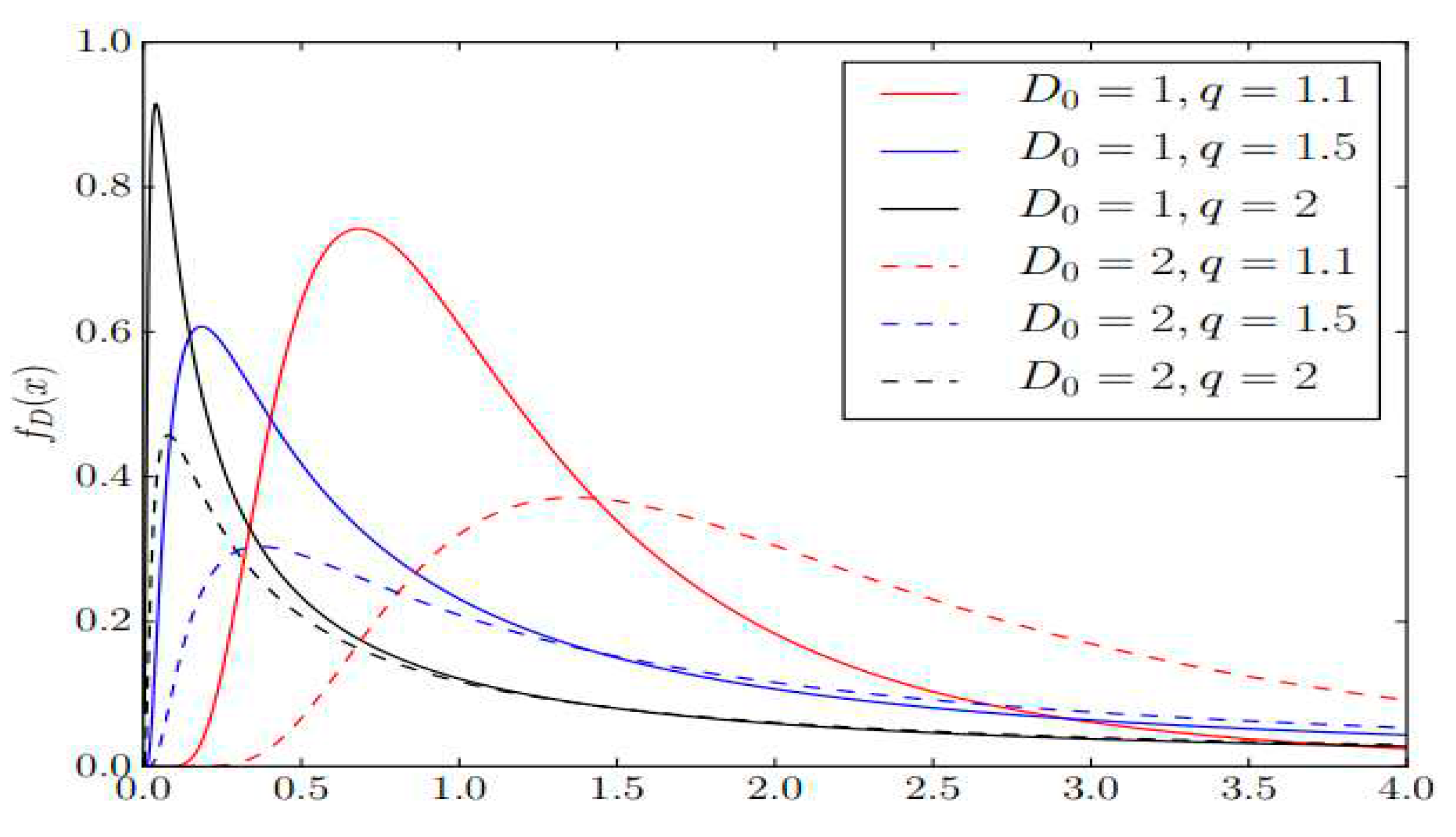
where   B ( t ) is a Brownian motion, and D is a random variable that is independent of B t . If the probability density function, f D ( x ) , of D is given by:
f D x = δ ( x D 0 ) (1.6)
D is a constant. Suppose that [43]:
D D 0 ν V 2   g ( V ) (1.7)
X t X 0 ν t D t Z (1.8)
D 0 t Z V ν (1.9)
Most importantly, (1.7) can be re-written as:
f D x = f V ( g 1 ( x ) )   d d x g 1 ( x )
= D 0 ( ν 4 ) ν ( ν 2 ) x ( ν 4 + 1 ) 2 ν 2 + 1 Γ ( ν 2 ) e ( ν D 0 2 x ) (1.10)
Figure 3. Several plots of f D ( x ) for several combinations of q ,   ν = 3 q q 1 and D 0 (c.f. [41]).
Preprints 97255 g003
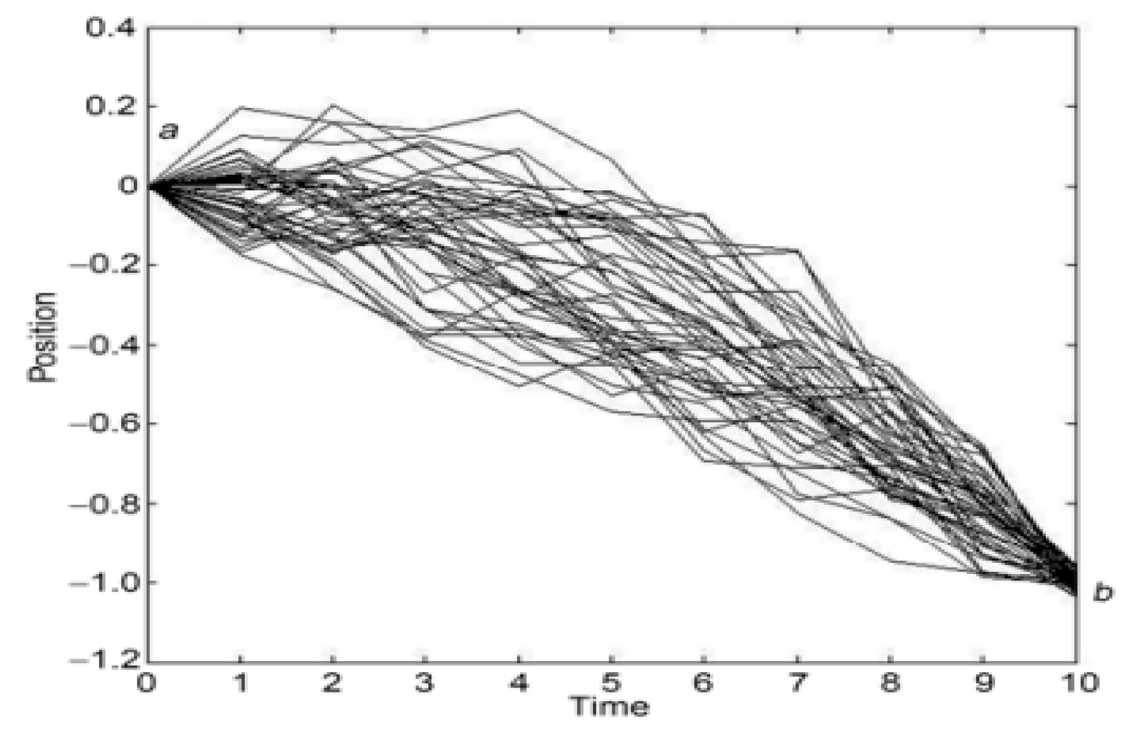
An idealised approximation to real random dynamics, known as Brownian motion, has been the subject of intense research over an extended temporal period [44,45,46,47,48,49,50,51,52,53,54,55,56]. A numerical simulation of a particle's route is shown in Figure 4.

1.4. Polygamma functions

The classical Euler gamma function may be defined for by R z > 0 by
Γ z = 0 y z 1 e y d y (1.11)
The digamma function, ψ z reads as:
ψ z = d d z l n Γ z = Γ ' z Γ z , ψ 1 = e (1.12)
The derivatives ψ ' z a n d ψ ' ' z ( ψ 1 z a n d ψ 2 z r e s p e c t i v e l y ) are called the trigamma and tetragamma functions respectively.
The Trigamma function, ψ 1 z is determined by[58]
ψ 1 z = n = 0 1 ( n + z ) 2 (1.13)
where ψ 1 z s a t i s f i e s ψ 1 1 = π 2 6 ( c . f . , 58 )
clearly, ψ 2 z solves (1.13) [59]
ψ 2 z = 2 n = 0 1 ( n + z ) 3 (1.14)
This paper contributes to:
  • The above discussion clearly demonstrates the significance of our novel approach as using the powerful tool of IG will open new grounds by looking for the first time (GB) as a manifold, by which we will directly determine visualization of (GBM) and searching in more depth for the temporal paths of the parameters of (GBM). Furthermore, IG technique is used to analyse (GBM) as well as the derivation of the corresponding curvature tensors, which physically describe the geometric shape of (GBM). More importantly, this clarifies the fact that Ig provides such an analysis of (GBM) which is impossible to be done by any other mathematical approach.
  • The new discovery of the informational geometric equations of motion (IGEMs) for (GBM)as well as obtaining the solutions of these equations.
  • Further advancements in the current paper are made by providing the information theoretic impact on the devised path of motion characterizing IGEMs.
  • Included are the physical applications and explanations of Gaussian and Ricci curvatures.
  • Providing a cutting-edge method for using computational information geometry to visualise queueing systems that has been suggested.
  • The creation of a novel quantitative approach to ascertain GBM’s temporal dynamics for the first time ever.
The rest of this paper is organised as follows: Section 2 presents preliminary definitions associated with (IG). The FIM and its inverse as well as the Fisher information metric for the Generalized Brownian Motion Manifold (GBM) are introduced in Section 3. The α (or ( α ) )-connection of the Generalized Brownian Motion Manifold (GBM)is obtained in Section 4. The GEs, KD and JD (c.f., [60]) of the Generalized Brownian Motion Manifold (GBM) are obtained in Section 5, numerical solutions to the devised GEs are obtained by using Rung-Kutta method of order 4 and numerical experiments are determined to illustrate the physical interpretations of our solutions. The structured proofs of calculating the 0-Gaussian curvature as well as the investigation of the developability of Generalized Brownian Motion Manifold (GBM) and showing that GBM has a non-zero Ricci curvature (RC) tensor are devised in Section 6. The exponential matrix analysis of the Generalized Brownian Motion Manifold (GBM) is obtained in Section 7. Conclusions and future research directions are included in Section 8. Full illustration of Rung-Kutta method of order 4 is provided in the Appendix.

2. Main Definitions in IG

2.1. Preliminary Definitions
Definition 2.1 Statistical Manifold (SM) 
An SM is referred to as M = { p ( x , θ ) | θ Θ } [60],with a probability density function p ( x , θ ) , and θ = ( θ 1 , θ 2 , . . , θ n ) Θ as the manifold M’s coordinates.
Definition 2.2 Potential Function 
The potential function   Φ θ (c.f., [60]) is the coordinates only part of ( l n ( ( p x , θ ) (c.f., (2.1)).
Definition 2.3 FIM, namely [ g i j ] 
[ g i j ](c.f., [61]) reads as:
g i j = 2 θ i θ j Φ θ , i , j = 1,2 , , n   (2.1)
Definition 2.4 FIM’s inverse 
[ g i j ] inverse (c.f.,[60]) reads as:
[ g i j ] = ( [ g   i j ] ) ) 1 = a d j g i j ,   = d e t g i j             ( 2.2 )
The arc length function reads:
( d s ) 2 = i , j = 1 n g i j ( d θ i ) ( d θ j )   (2.3)
Definition 2.5 α -Connection, ( α ) , α R [61]
( α ) reads
Γ i j , k ( α ) = ( 1 α 2 ) ( i j k ( Φ θ ) ) (2.4)
Definition 2.6 Kullback’s Divergence (KD), 𝑲𝒑, 𝒒 
K p , r (c.f., [60]) reads as :
K p , r = p x ; θ p l n p x ; θ p r x ; θ r d x   (2.5)
The J-divergence reads as :
J p , r = ( p x ; θ p r ( x ; θ r ) ) l n p x ; θ p r x ; θ r d x   (2.6)
Definitions 2.7 Geodesic Equations (GEs) 
1. The GEs of manifold M with coordinate system θ = θ 1 , θ 2 , . . , θ n c.f., [60]) are defined by
d 2 θ k d t 2 + Γ i j k 0 d θ i d t ( d θ j d t ) = , i , j = 1,2 , , n , Γ i j k α = Γ i j , s α g s k ,   i ,   j ,   k ,   s   =   1 , 2 , , n (2.7)
2.[60] A path θ = θ t   minimising the total energy E = E θ must satify :
d d t 2 L ( d θ j d t ) θ j = 0 (2.8)
FIM’s inverse defines   g i j (IM) so that :
k = 1 n   g i k   g k j = δ i j (2.9)
where δ i j = 1 ,     i = j 0 ,   o t h e r w i s e (c.f., [60])
5. Lemma [60] GEs are the equations of motion
L = L θ , d θ d t
Such that
d 2 θ i d t 2 + j , k = 1 n Γ j , k i d θ j d t d θ k d t = 0 (2.10)
Hence, GEs are interpreted physically as the information geometric equations of motion (IGEMs).
Definition 2.8 
1. The α c u r v a t u r e R i e m a n n i a n
Tensors,   R i j k l ( α ) (c.f., [58]) are defined by
  R i j k l ( α ) = j Γ i k s α i Γ j k s α g s l + Γ j t , l α Γ i k t α Γ i t , l α Γ j k t α (2.11)
where Γ i j k α = Γ i j , s α g s k
2.   R i k ( α ) define the Ricci tensors (c.f.,[58]),
  R i k ( α ) =   R i j k l ( α ) g j l (2.12)
3. K i j i j ( α ) reads as (c.f.,[60])
K i j i j ( α ) = R i j i j ( α ) g i i g j j ( g i j ) 2 (2.13)
K 1212 α = K α defines the α   G a u s s i a n c u r v a t u r e (c.f., [60])
K α = R 1212 ( α ) d e t g i j (2.14)
4. The Ricci Tensor (c.f.,[60]) defines the contraction of R i j k l ( α ) (c.f.,[60]).
5. The difference between a geodesic ball's volume on the surface and its volume in Euclidean space is known as the oriented Riemannian Manifold M ’ s Ricci curvature Tensor (c.f., [62]).
6. The volumes’ evolution is contracted by the Ricci curvature RC) (c.f., [63]). The Bonnet Myers theorem (c.f., [64]) states that when Ricci curvature is positive, the Riemannian manifold has a smaller diameter and is more positively curved than a sphere.
Figure 5. Visualizing Ricci curvature (c.f., [65]).
Preprints 97255 g005
Definition 2.9 [66]
1. Given a n-dimensional vector x is and A is a nxn matrix, such that
d x d t = A x (2.15)
e A reads:
e A = i = 0 A i i ! = I + A + A 2 2 ! + + A k k ! + (2.16)
solves (2.15).
2. Let
Φ δ = det A δ I (2.17)
Φ δ = 0 (2.18)
The solution of (2.18) are referred to as A’s eigen values such that:
A x = δ   x (2.19)
Notably,   e A   may be re-written as:
  e A   = T   e D   T 1   (2.20)
where D is the diagonal matrix of eigen values of A, and T is matrix having of the corresponding eigen vectors of A as its columns.
Definition 2.10 
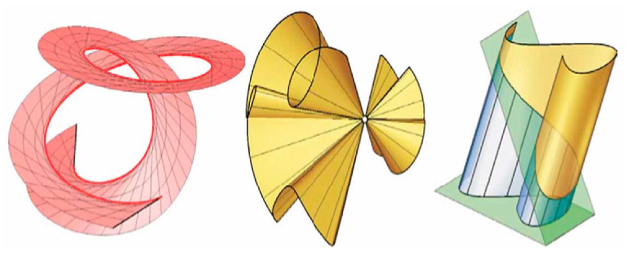
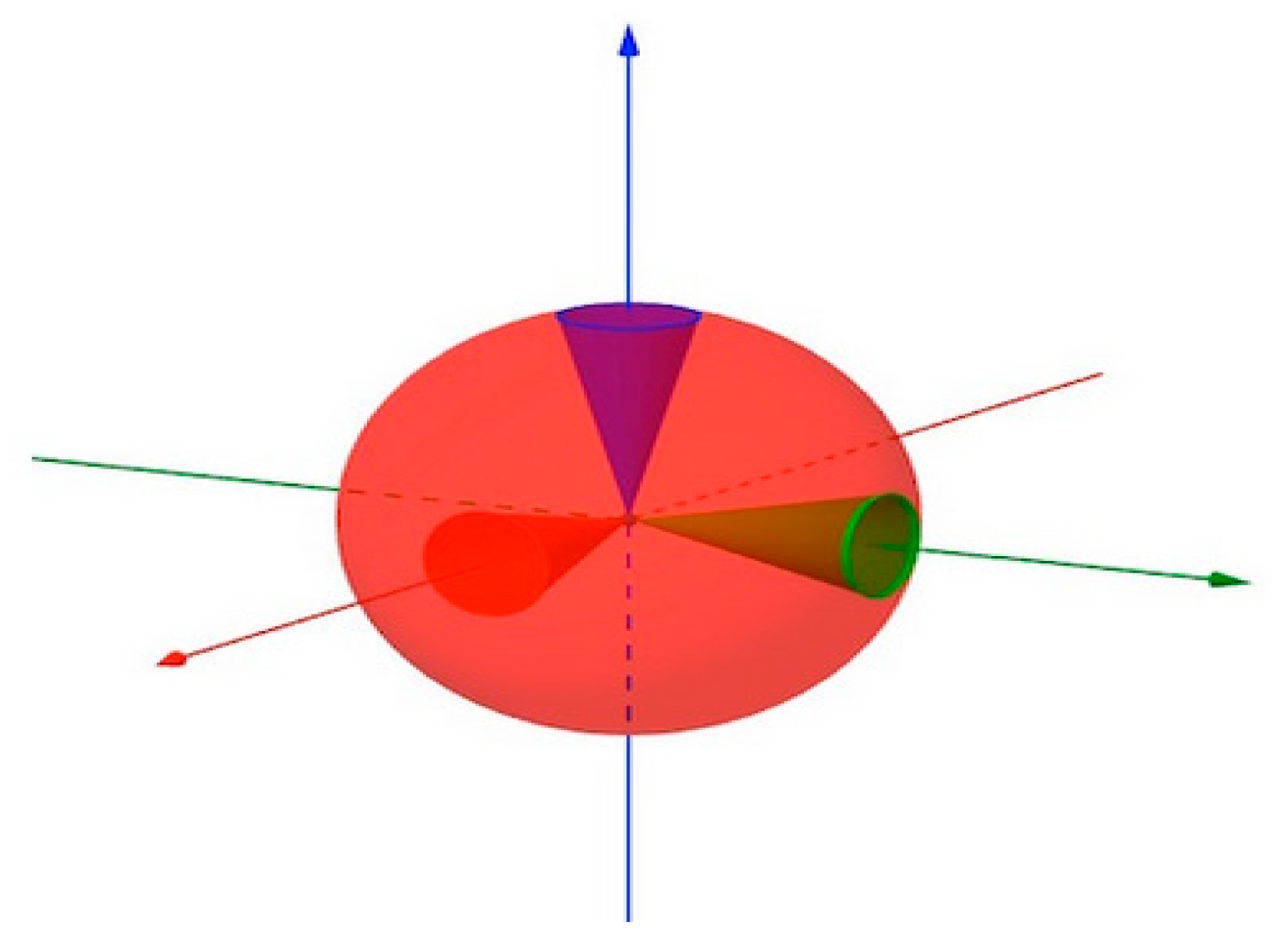
A unique type of ruled surface known as a developable surface has a Gaussian curvature of 0 and can be mapped onto a plane surface without causing any curve distortion; a curve drawn from such a surface onto a flat plane stays the same (c.f., [67]).
Figure 6. Three kinds of developable surfaces: Tangential on the left, Conical on the centre and on the right, Cylindrical (c.f., [67]).
Preprints 97255 g006
In the following, a brief overview of Gaussian and Mean Curvatures (c.f.,[68]).

2.2. Gaussian and Mean Curvatures[68]

Definition 2.11 (Mong Patch Technique) 
1.Let K 1 and K 2 be the principal curvatures of a surface patch δ u , v .   The Gaussian Curvature K G of δ is
K G = K 1 K 2 (2.21)
and its Mean Curvature is
H = 1 2 ( K 1 + K 2 ) (2.22)
2. For a Mong patch z = f x , y , K G and H are given by
K G = L N M 2 E G F 2 (2.23)
and its Mean Curvature reads
H = 1 2 ( L G 2 M F + N E E G F 2 ) (2.24)
with   E = ( f x ) 2 ,   F = f x y ,   G = ( f y ) 2 ,   L = 2 f x 2 ,   M = f x y ,   N = 2 f y 2

2.2.1. Classification of Surface Points

The physical interpretation of the sign of K G at a point r on a surface S is:
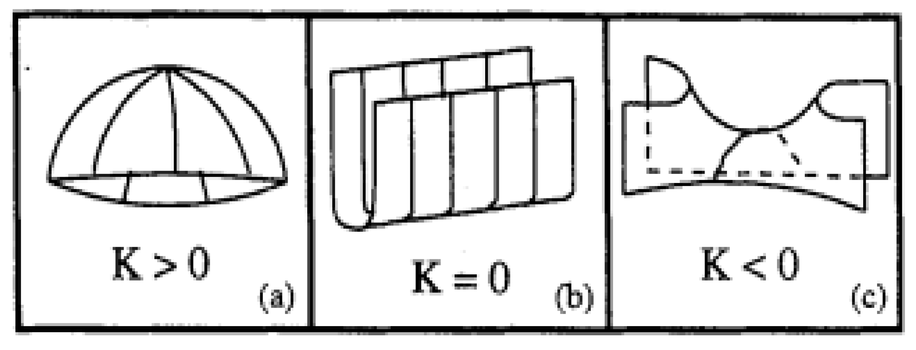
1. K G > 0 The principal curvatures K 1 and K 2 have the same sign at r . An illustrative example is given by Figure 7.
2. K G > 0 The principal curvatures K 1 and K 2 have opposite signs at r.
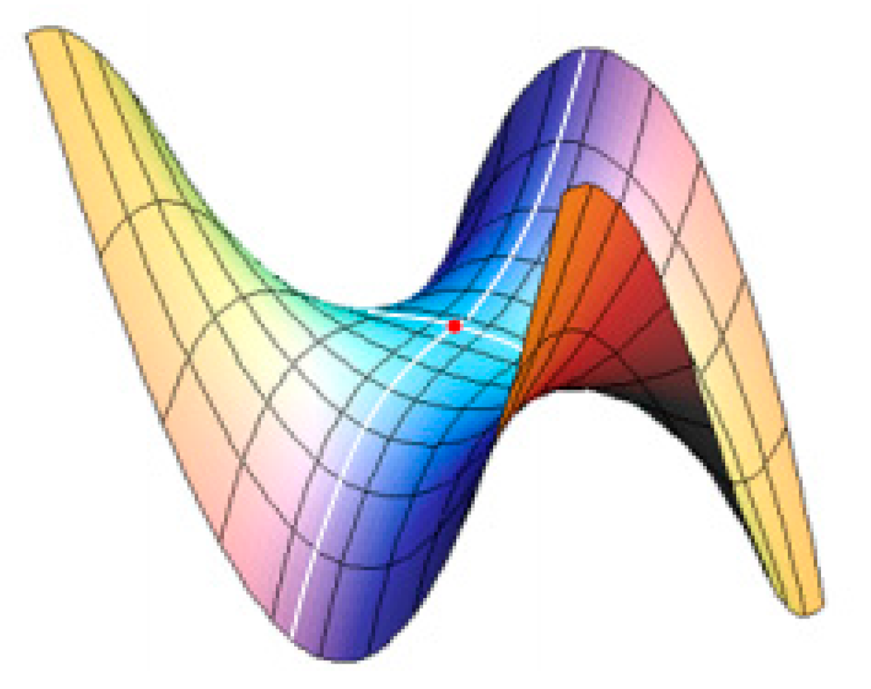
3. K G > 0 , point in the plane and the origin of a monkey saddle z = x 3 3 x y 2 as in Figure 8, are both planar points, but they have quite different shapes.
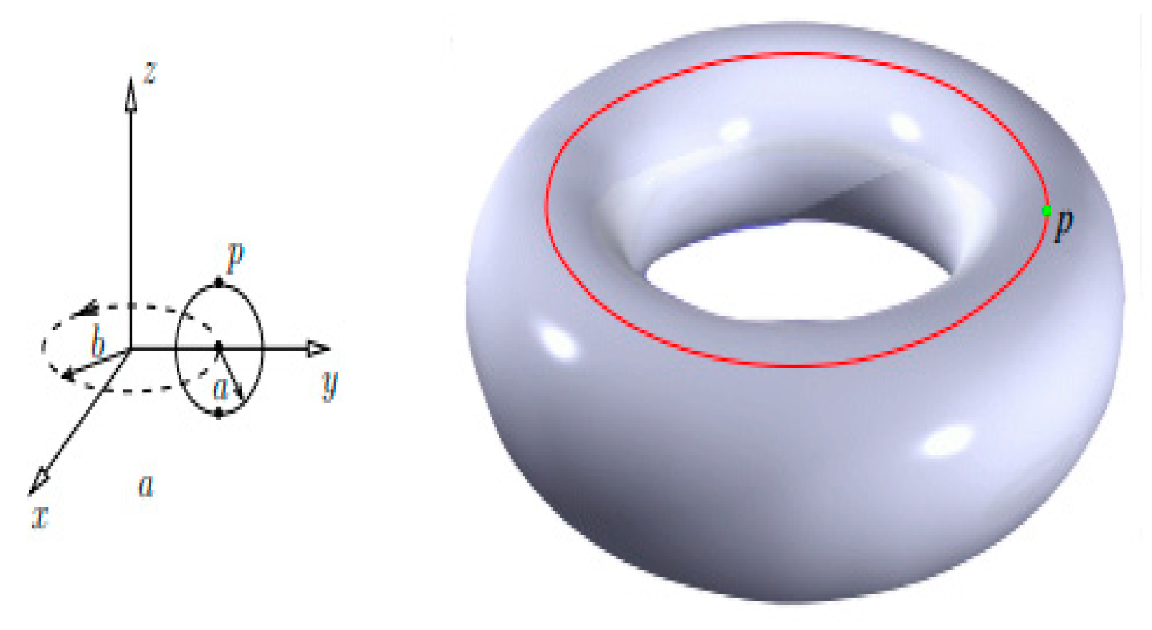
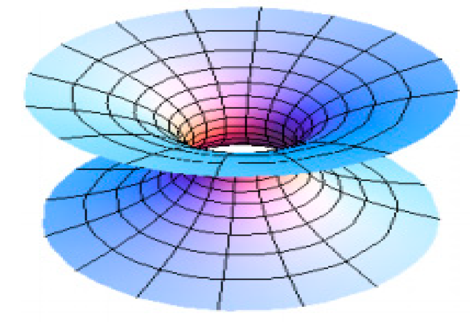
A torus as shown in Figure 9. Minimal surfaces have Gaussian curvature K G 0 . The catenoid in Figure 10 is a minimal surface.

2.3. Different Approach to Gaussian and Mean Curvatures (Angular Technique)[69]
A new formulation (c.f., [69]) is introduced for Gaussian Curvature K G and the Mean Curvature is H are defined as
K G = K 1 K 2 (2.25)
and H = 1 2 ( K 1 + K 2 ) (2.26)
w i t h   K 1 and K 2 as the principal curvatures are determined by:
K 1 = B 11 ( 1 + ( f x 1 ' ) 2 ) 3 2 , K 2 = B 22 ( 1 + ( f x 2 ' ) 2 ) 3 2 (2.27)
where x 3 = f ( x 1 , x 2 ) defines the shape of the surface. x 1 ' and x 2 ' are parallel to the directions of the principal curvature, which are rotated through an angle with respect to x 1 a n d x 2 , and
f x 1 ' = c o s f x 1 s i n f x 2 (2.28)
f x 2 ' = s i n f x 1 + c o s f x 2 (2.29)
B 11 = 2 f x 1 2 c o s 2 2 2 f x 1 x 2 s i n c o s + 2 f x 2 2 s i n 2 = 2 f x 1 ' 2 (2.30)
B 22 = 2 f x 1 2 s i n 2 + 2 2 f x 1 x 2 s i n c o s + 2 f x 2 2 c o s 2 = 2 f x 2 ' 2 (2.31)
t a n 2 = 2 ( 2 f x 1 x 2 ) ( 2 f x 1 2 2 f x 2 2 ) (2.32)
Where structures appear on a surface is indicated by a Gaussian curvature contour map. A surface is considered to have twofold curvature if both of its primary curvatures are non-zero [70].
Figure 11. (c.f., [69]). (a) K G > 0, (b) K G = 0 and (c) K G < 0.
Preprints 97255 g011
This paper contributes to:
i) The FIM and its inverse as well as the FIM for (GBM) are introduced.
ii) A novel GBM’s α [61] are devised. These novel derivations are used to determine the GEs for the coordinates of (GBM). These equations are considered as analogues to the equations of motion in dynamics. In other words, the information geometric equations of motion are devised for the coordinates of the (GBM) manifold. iii) The GEs, the KD, and the JD of (GBM) are determined. iv) (GBM) could be compressible or non-solenoidal(for a more detailed survey, consult [71]). Moreover, for first time ever, the necessary and sufficient mathematical requirement that characterizes the developability of GBM manifold is devised. Also, a novel sufficient and necessary conditions which characterizes the regions where the surface describing GBM is minimal is determined. v) The exponential of the FIM for GBM solves d x   d t = Ax.

3. The Fim and Its Inverse for (GBM)

Theorem 3.1 
For GBM manifold, we have
(i)The FIM is given by:
[ g i j ] = 1 ν + 1 4 ψ 1 ( ν 2 ) 1 4 D 0 1 4 D 0 ν 4 D 0 2 (3.1)
(ii) ( d s ) 2 = ( 1 ν + 1 4 ψ 1 ( ν 2 ) ) d ν 2 1 4 D 0 ( d ν ) ( d D 0 ) + ν 4 D 0 2 d D 0 2 (3.2)
(iii) IFIM reads as:
[ g i j ] = ( [ g i j ] ) ) 1 = a d j g i j
= 1 Δ ν 4 D 0 2 1 4 D 0 1 4 D 0 1 ν + 1 4 ψ 1 ( ν 2 ) (3.3)
with Δ = 1 16 D 0 2 ( ν ψ 1 ν 2 5 )
Proof 
(i)We have f D x = = D 0 ( ν 4 ) ν ( ν 2 ) x ( ν 4 + 1 ) 2 ν 2 + 1 Γ ( ν 2 ) e ( ν D 0 2 x ) (c.f., (1.10)
L x ; θ = l n f D x ; θ
= ( l n Γ ν 2 1 + ν 2 l n 2 ν D 0 2 x + ν 4 l n D 0 + ν 2 l n ν ( 1 + ν 4 ) l n x ) ,  
θ = ( θ 1 ,   θ 2 ) = ( ν ,   D 0 ) (3.4)
Φ θ = ( l n Γ ν 2 + 1 + ν 2 l n 2 ν 4 l n D 0 ν 2 l n ν ) ,   (3.5)
Thus,
1 = Φ ν = ( 1 2   l n 2 + 1   2 ψ ( ν 2 ) 1 2 l n ν ) (3.6)
2 = Φ D 0 = ν 4 D 0 (3.7)
1   1 = 2 Φ ν 2 = 1 ν + 1 4 ψ 1 ( ν 2 )   (3.8)
1 2 = 2 1 = 1 4 D 0 (3.9)
2 2   = ν 4 D 0 2 (3.10)
Therefore, the FIM is given by
[ g i j ] = 1 ν + 1 4 ψ 1 ( ν 2 ) 1 4 D 0 1 4 D 0 ν 4 D 0 2 ( c . f . , (3.1)), which proves (i).
(ii) is immediate.
(iii) We must show that:
Δ = det g i j = 1 16 D 0 2 ν ψ 1 ν 2 5 0 .
If q ( 1 < q < 3 ) , ν = 3 q q 1 , then the extensivity of ν follows, and ν > 1 . Assuming that Δ = det g i j = 1 16 D 0 2 ν ψ 1 ν 2 5 = 0 . Then, without loss of generality, let n = 1 in (1.13).Hence, it follows by the assumption that:
ν ψ 1 ν 2 5 = ( ν 1 ν 2 2 + 1 1 + ν 2 2 5 ) = 0 (3.11)
Therefore,
5 ν 3 + 12   ν 2 + 4 ν 16 = 0 (3.12)
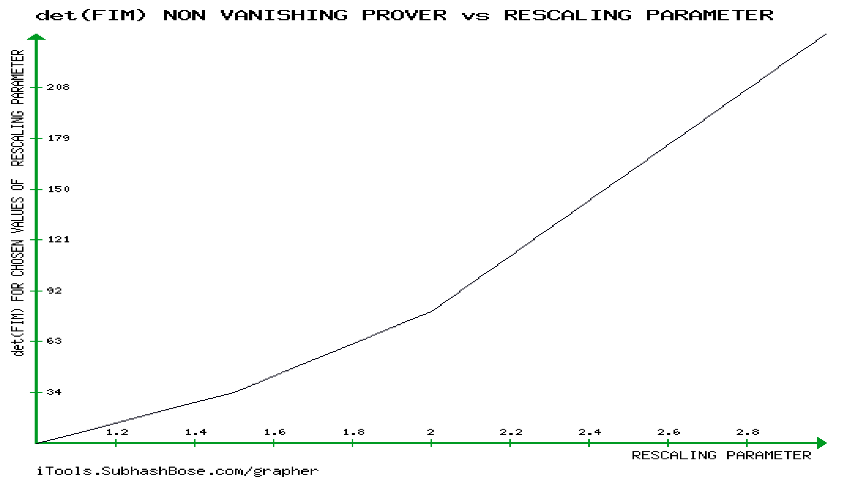
Let’s call 5 ν 3 + 12   ν 2 + 4 ν 16 , the non- vanishing prover(NVP). More importantly, NVP 0 (see Figure 12), debunking (3.12), that is :
Δ = det g i j = 1 16 D 0 2 ν ψ 1 ν 2 5 0 .
Figure 12 shows that det(FIM) is non-zero. For higher level values of n 2 , the case is always true as it is obvious that the values of ν ψ 1 ν 2 will be more increasing. This shows that the inverse of Fisher Information Matrix of GBM exists. The remaining proof of (iii) follows.
It is notable to mention that all the novel findings in this paper involve digamma, Trigamma and Tetragamma functions which indicates another physical importance of our breakthrough as it unifies IG with (GBM) together with many other physical as well as mathematical sciences.

4. The α (OR ( α ) )-Connection of (GBM)

By definition (2.4), we have
Γ 11,1 ( α ) = 1 α 2 ( 1 ν 2 + 1 8 ψ 2 ( ν 2 ) ) (4.1)
Γ 11,2 ( α ) = Γ 12,1 ( α ) = Γ 21,1 ( α ) = 0 (4.2)
Γ 12,2 ( α ) = 1 α 8 D 0 2 = Γ 22,1 ( α ) = Γ 21,2 ( α ) (4.3)
Γ 22,2 ( α ) = α 1 ν 4 D 0 3 (4.4)
Furthermore, the following expressions follow:
Γ 11 1 α = Γ 11,1 α g 11 + Γ 11,2 α g 21 ,
which is after some lengthy calculations:
Γ 11 1 α = 1 α ν 8 Δ D 0 2 ( 1 ν 2 + 1 8 ψ 2 ( ν 2 ) ) ,   Γ 11 1 0 = ν 8 Δ D 0 2 ( 1 ν 2 + 1 8 ψ 2 ( ν 2 ) ) (4.5)
Γ 12 1 α = Γ 21 1 α = 1 α 32 Δ D 0 3   ,   Γ 12 1 0 = Γ 21 1 0 = 1 32 Δ D 0 3 (4.6)
Γ 22 1 α = α 1 ν 32 Δ D 0 4 ,   Γ 22 1 0 = ν 32 Δ D 0 4 (4.7)
Γ 11 2 α = 1 α 8 Δ D 0 2 ( 1 ν 2 + 1 8 ψ 2 ( ν 2 ) ) , Γ 11 2 0 = 1 8 Δ D 0 2 ( 1 ν 2 + 1 8 ψ 2 ( ν 2 ) ) (4.8)
Γ 12 2 α = Γ 21 2 α = 1 α 8 D 0 2 1 ν + 1 4 ψ 1 ν 2 ,   Γ 12 2 0 = Γ 21 2 0 = 1 8 D 0 2 1 ν + 1 4 ψ 1 ν 2 (4.9)
Γ 22 2 α = 1 α 32 Δ D 0 3 ( 9 2 ν ψ 1 ν 2 ) , Γ 22 2 ( 0 ) = 1 32 Δ D 0 3 9 2 ν ψ 1 ν 2 (4.10)
Using the above derivations, the GEs of the (GBM) can be devised, which are the information geometric equations of motion for the (GBM).

5. The GEs, the KD, and the JD of the (GBM). K D G B M and J D G B M

By the definition, the GEs should take the form:
d 2 θ k d t 2 + Γ i j k 0 d θ i d t ( d θ j d t ) = 0 , i , j = 1,2 , , n   (5.1)
G E S k = 1   reads as
d 2 ν d t 2 + Γ 11 1 0 d ν d t 2 + Γ 22 1 0 d D 0 d t 2 + Γ 12 1 0 + Γ 21 1 0 d ν d t d D 0 d t = 0   (5.2)
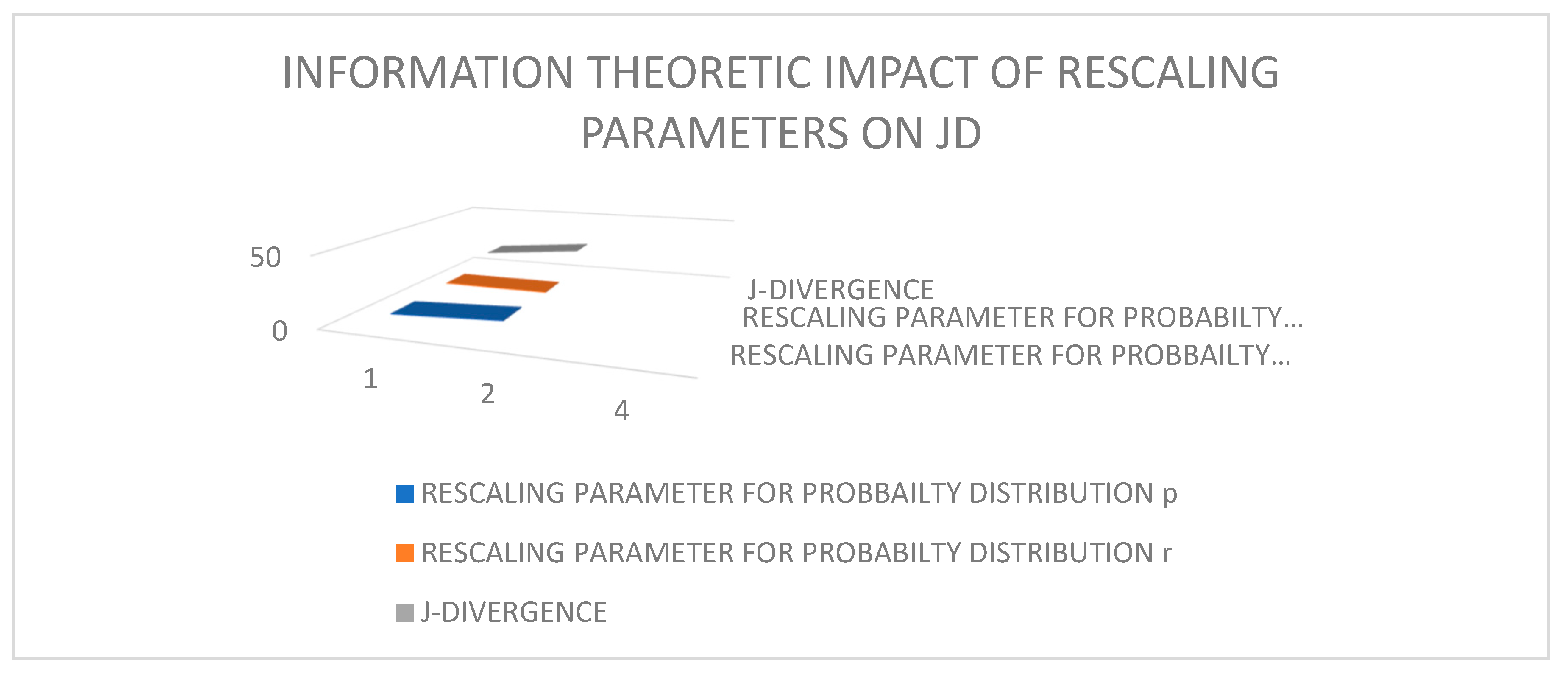
Equation (5.2) presents a family of families of equations of motion of the rescaling parameter, RP = ν which are dependent on the values of both the parameters ν and D 0 . One element of this family could be obtained by assuming that D 0 = 1 . Thus,
d 2 ν d t 2 + ν 8 Δ D 0 2 ( 1 ν 2 + 1 8 ψ 2 ( ν 2 ) ) d ν d t 2 = 0   (5.3)
with Δ = det g i j = 1 16 D 0 2 ν ψ 1 ν 2 5
This transform (5.3) to be :
d 2 ν d t 2 + 2 ν ν ψ 1 ν 2 5 ( 1 ν 2 + 1 8 ψ 2 ( ν 2 ) ) d ν d t 2 = 0   (5.4)
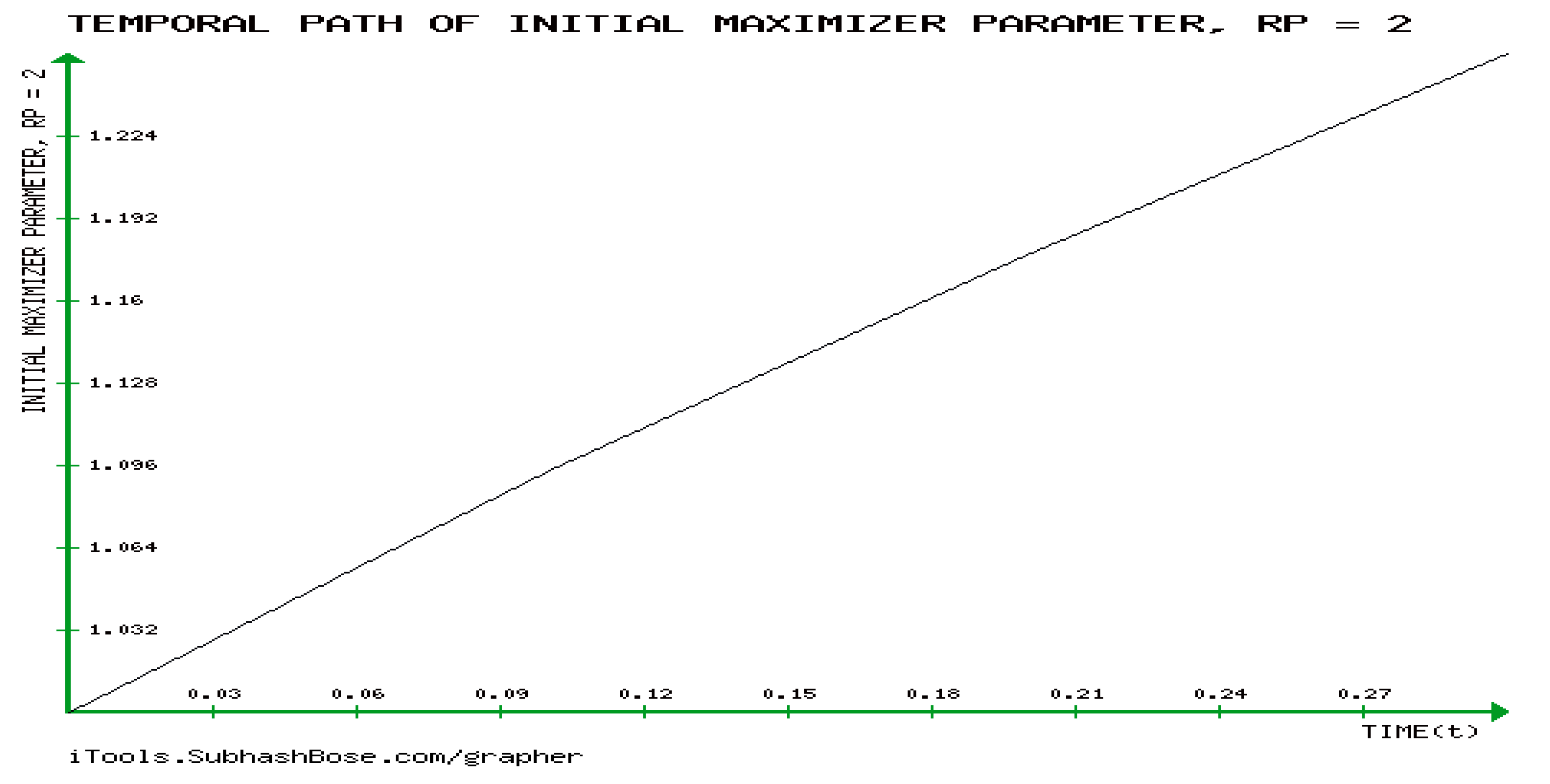
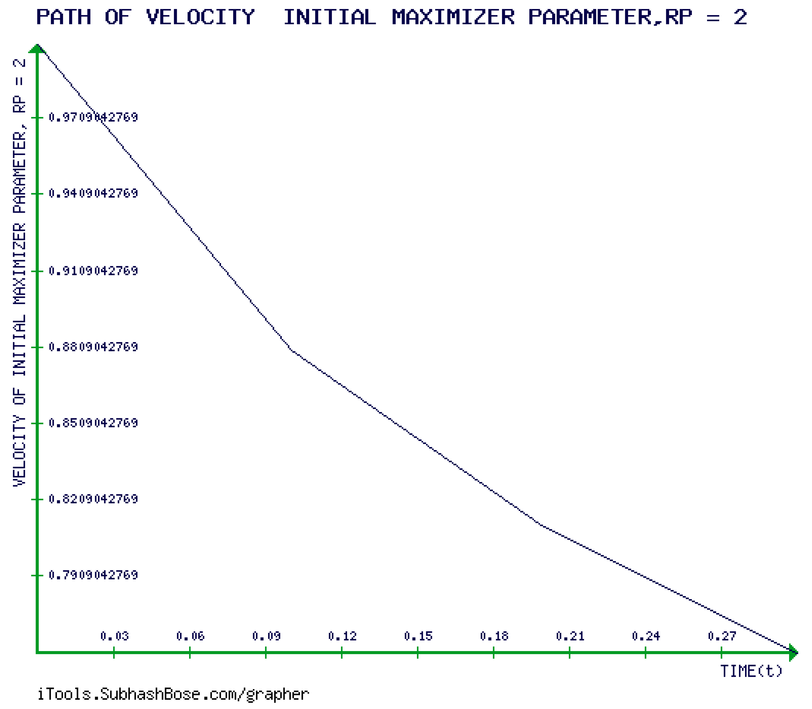
At k = 2, we have a family of families of equations of motion of the initial maximiser parameter, IMP = D 0 which are dependent on the values of both the parameters ν and D 0 . One element of this family could be obtained by assuming that ν = 2 ( o r   e q u i v a l e n t l y ,   q = 5 3 )there is a second set of GEs corresponding to the 2nd coordinate D 0 , namely:
d 2 D 0 d t 2 + 1 2 ψ 1 1 5 D 0 3 ( 9 4 ψ 1 1 ) d D 0 d t 2 = 0   (5.4)
By ψ 1 1 = π 2 6   ,   5.4 will take the form:
d 2 D 0 d t 2 + 1 π 2 15 D 0 3 ( 27 2 π 2 ) d D 0 d t 2 = 0   (5.5)
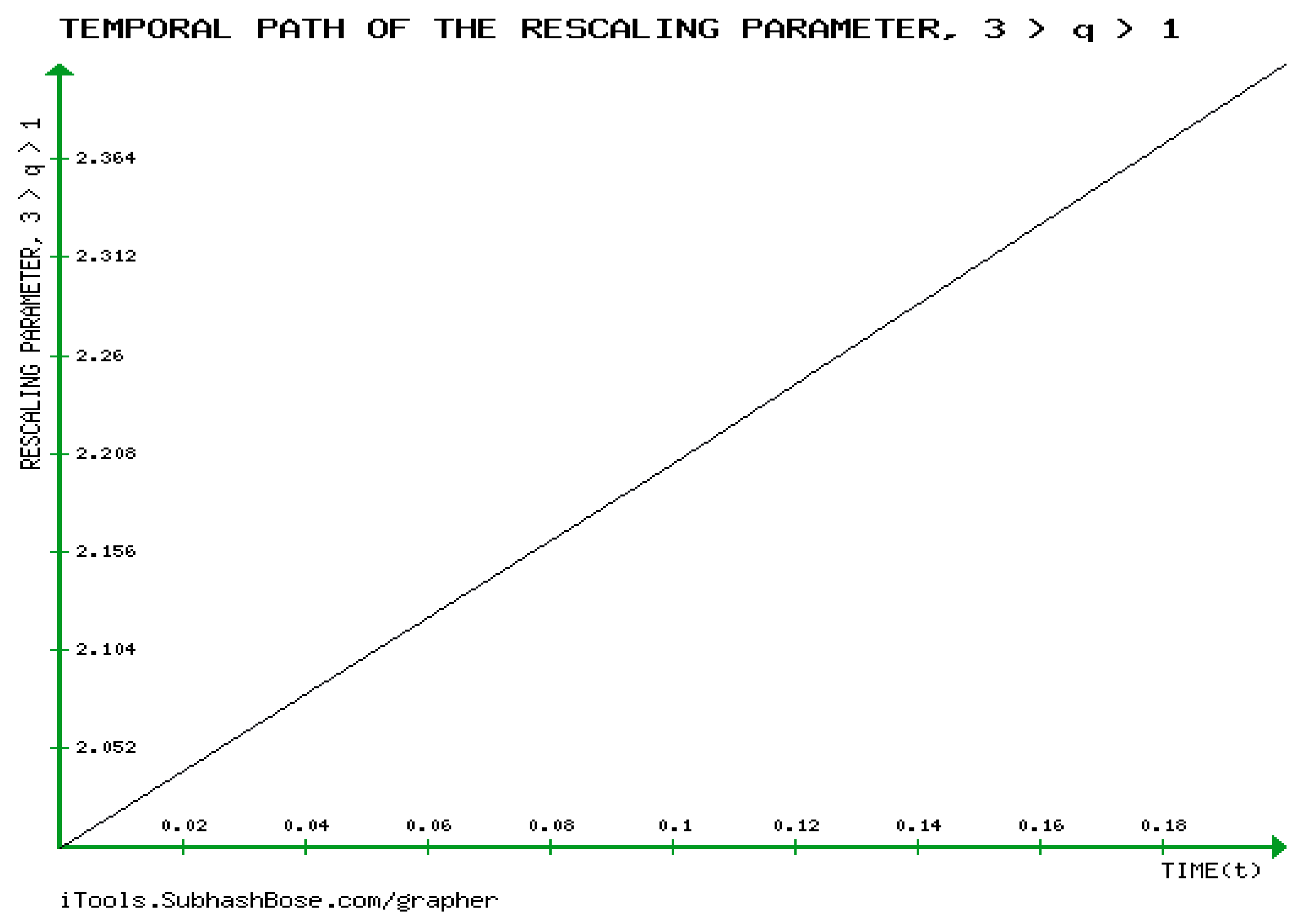
Using Rung-Kutta method of order 4, the numerical solution of (5.4) can be visualized for n = 10 ,   as in Figure 13 below.
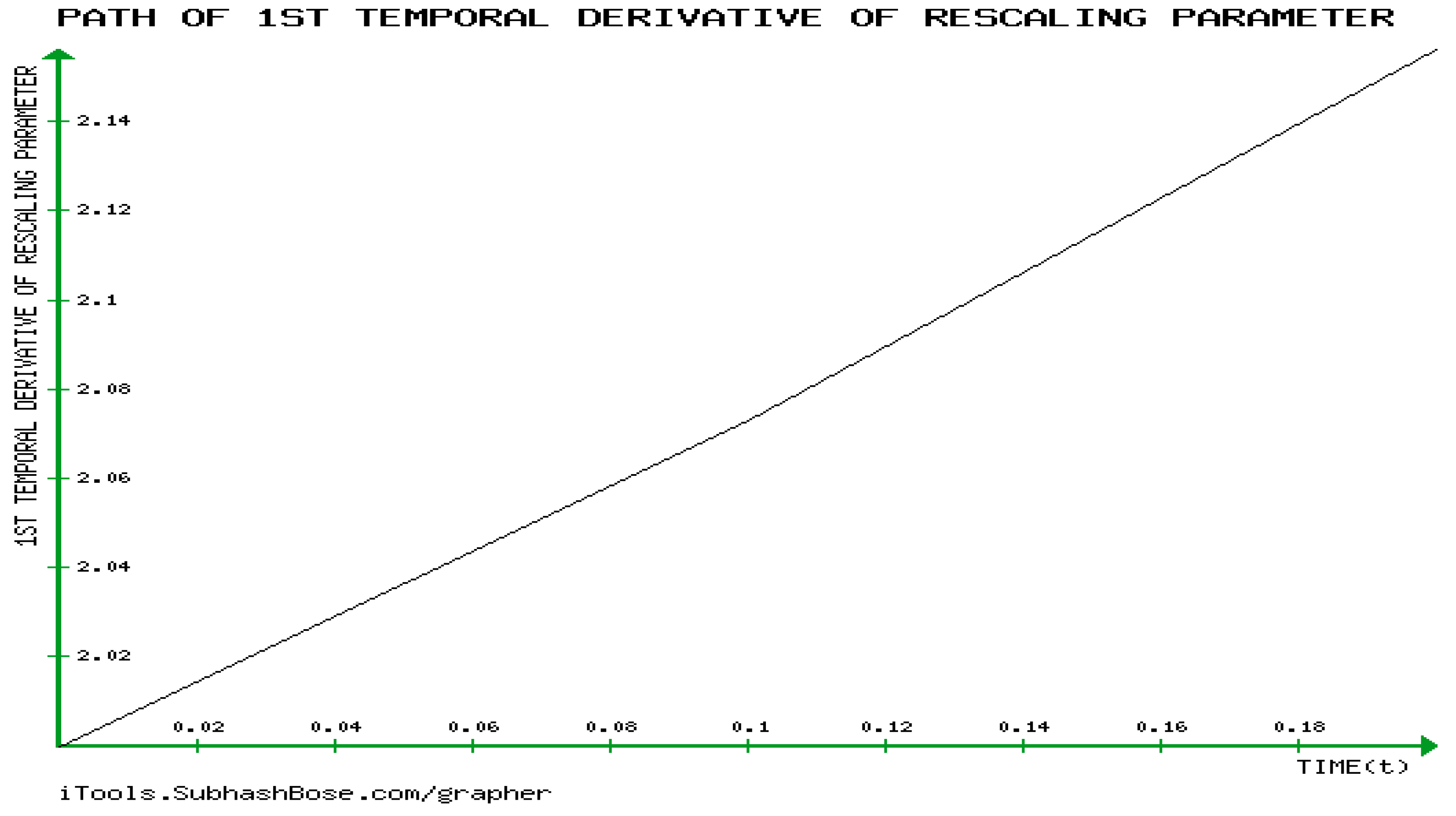
Following Figure 13 and Figure 14, the analysis of the dynamics of both the position of information theoretic rescaling parameter and its velocity shows an increase against time, which describes a form of unbounded motion. This also justifies the physical concept of (GBM). This also allows us for first time ever to capture the hidden dynamics of GBM from an IG viewpoint.
Analysis of the dynamics of both the position of information theoretic initial maximize (IMP) parameter and its velocity shows an increase against time in Figure 15 and Figure 16, a description of a form for an unbounded motion which justifies the physical concept of (GBM). Furthermore, the velocity of (IMP) decreases as time increase, which directly implies that the motion of the (IM) parameter will reach rest point at a certain time elapse. This also allows us for first time ever to capture the hidden dynamics of GBM from an IG viewpoint.
Figure 15. The temporal path of the velocity of the initial maximizes parameter.
Preprints 97255 g015
Figure 16. The temporal path of the velocity of the initial maximizer parameter(IMP), namely D 0
Preprints 97255 g016
Now, by (2.6), after some few algebraic calculations, the   K D G B M p , r reads as:
  K G B M ν p ,   ν r   , D 0 p , D 0 r = ( 2 ν p , ν r ) Γ ( ν r 2 ) ( ν p ν p ν r ν r ) ( D o p ν p D o r ν r ) 1 4 Γ ( ν p 2 )   (5.6)
Moreover, in a similar fashion, the   J D G B M p , r reads as
  J D G B M p , r =   K D G B M p , r +   K D G B M r , p = l n p x ; θ p r x ; θ r ( p x ; θ p r x ; θ r ) 0 (5.7)
(5.7) presents contributes to revealing that GBM manifold is compressible or non-solenoidal.
Getting more deeper with our mathematical calculations,
K G B M ν p ,   ν r   , D 0 p , D 0 r =
= ( 2 ν p ν r ) Γ ( ν r 2 ) ( ν p ν p ν r ν r ) ( D o p ν p D o r ν r ) 1 4 Γ ( ν p 2 ) + ( 2 ν r ν p ) Γ ( ν p 2 ) ( ν r ν r ν p ν p ) ( D o r ν r D o p ν p ) 1 4 Γ ( ν r 2 ) (5.8)
In what follows, we present some numerical experiments to illustrate the physical interpretations of our new findings.
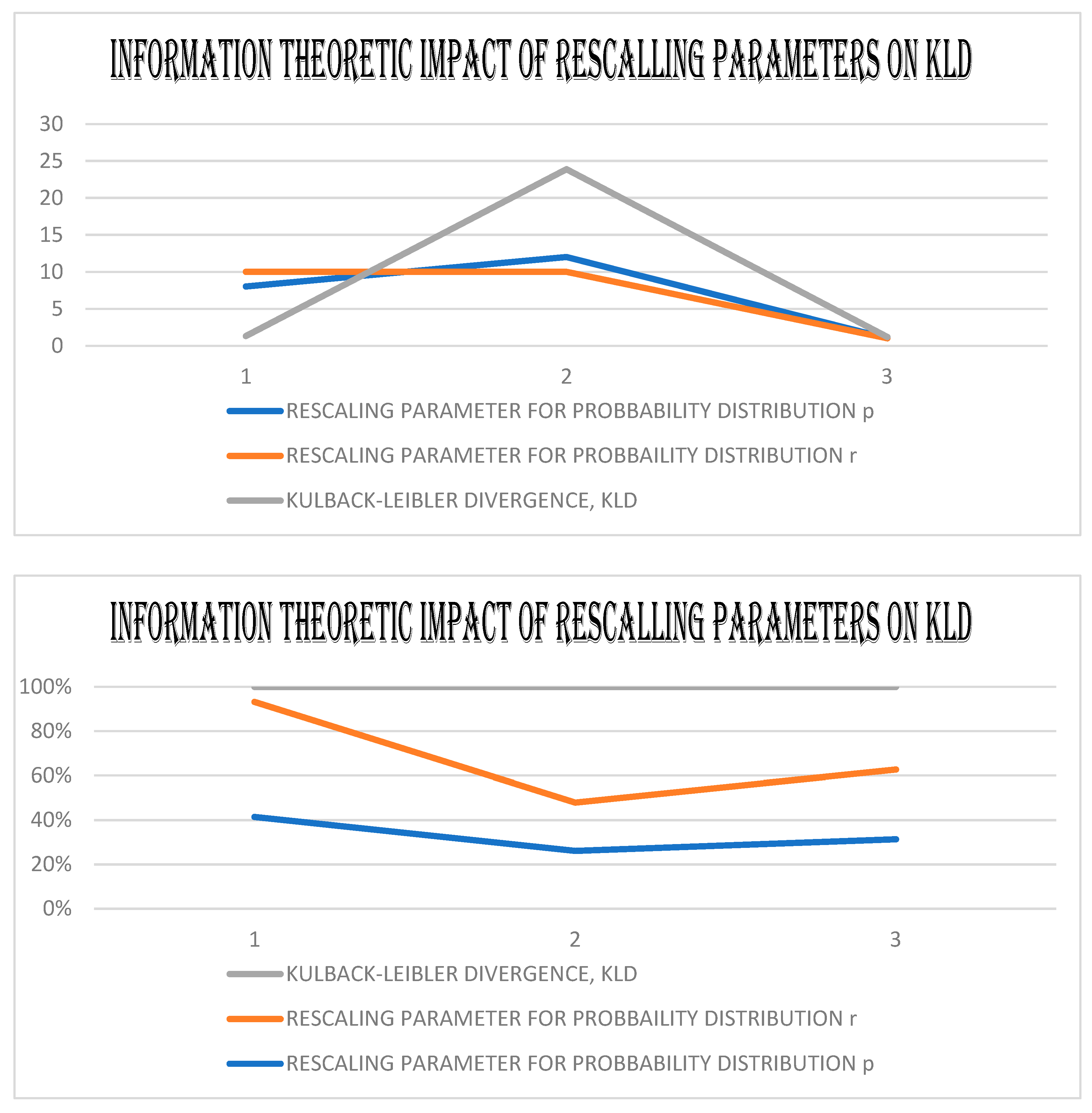
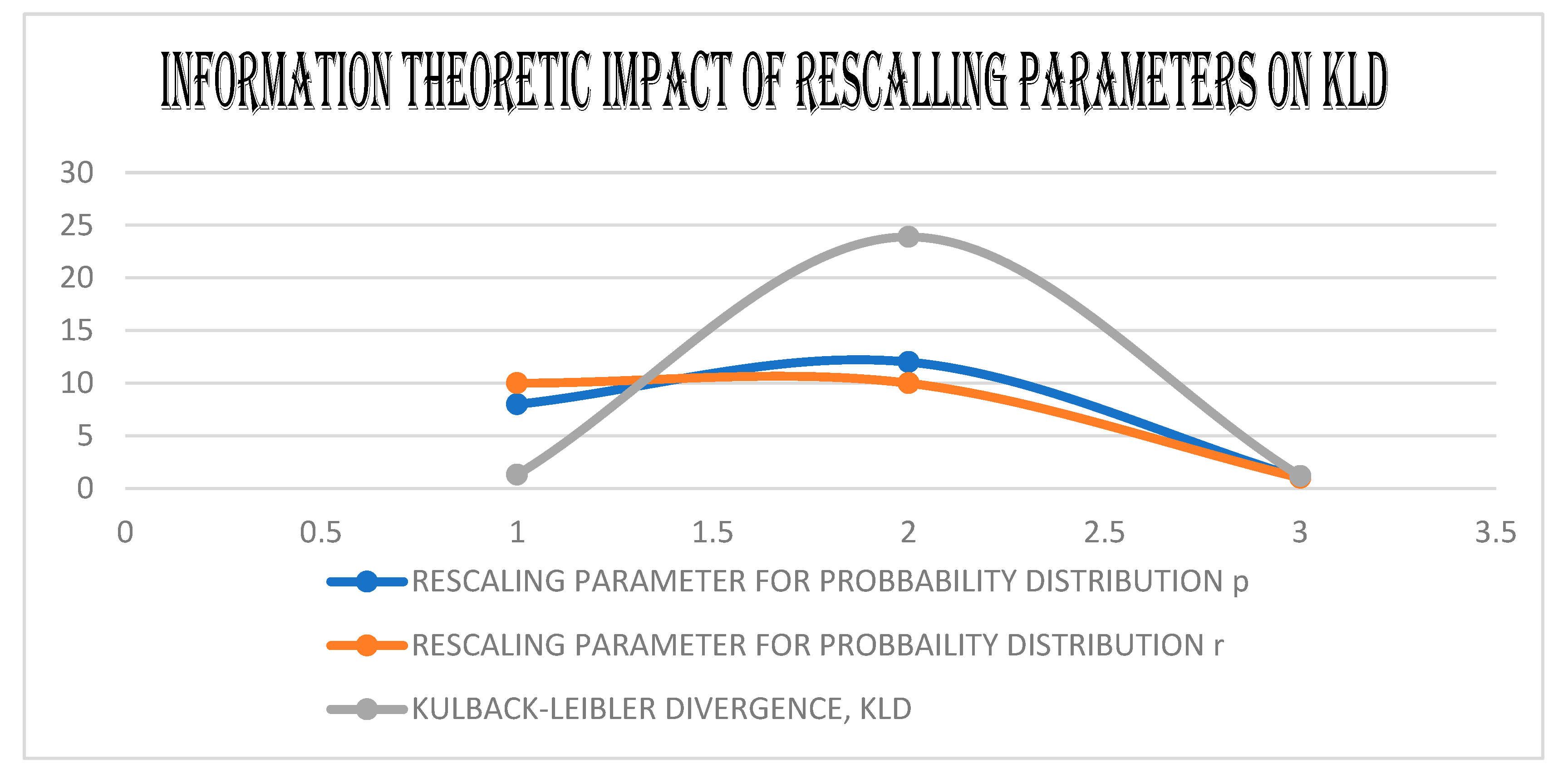
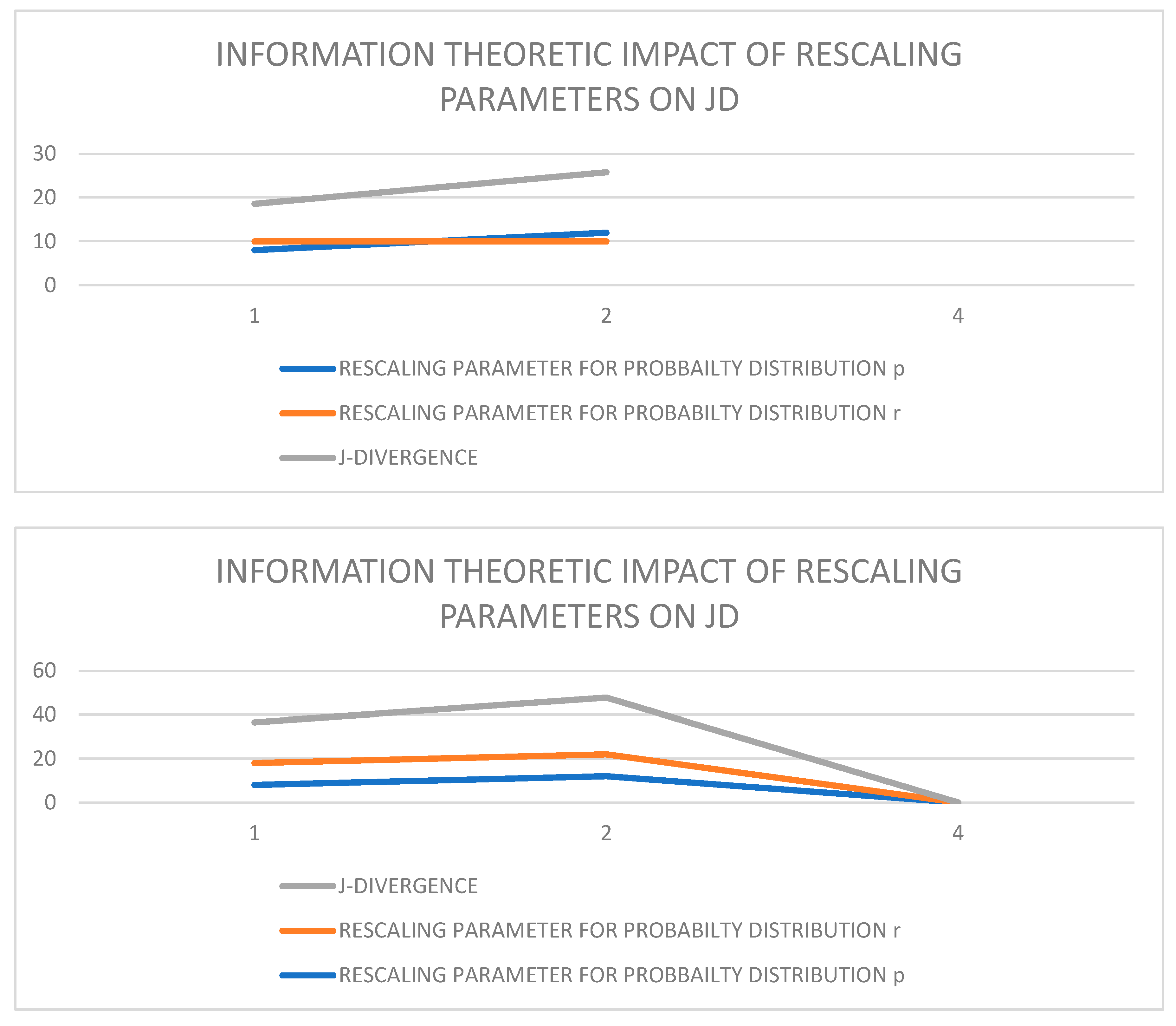
By Figure 17 and Figure 18, the analysis shows that the underlying KD and ID of GBM are influenced by the information theoretic impact of both rescaling and initial maximize parameters, ν   a n d D 0 This is shown by the path continuity of the above graphs of coordinates as well as their temporal velocities.

6. Novel Investigation of the Mathematical Requirements of the developabality of (GBM) , Calculating 0-Gaussian Curvature of GBM, and Showing that RICCI CURVATURE (RC) tENSOR of GBM is Non-Zero
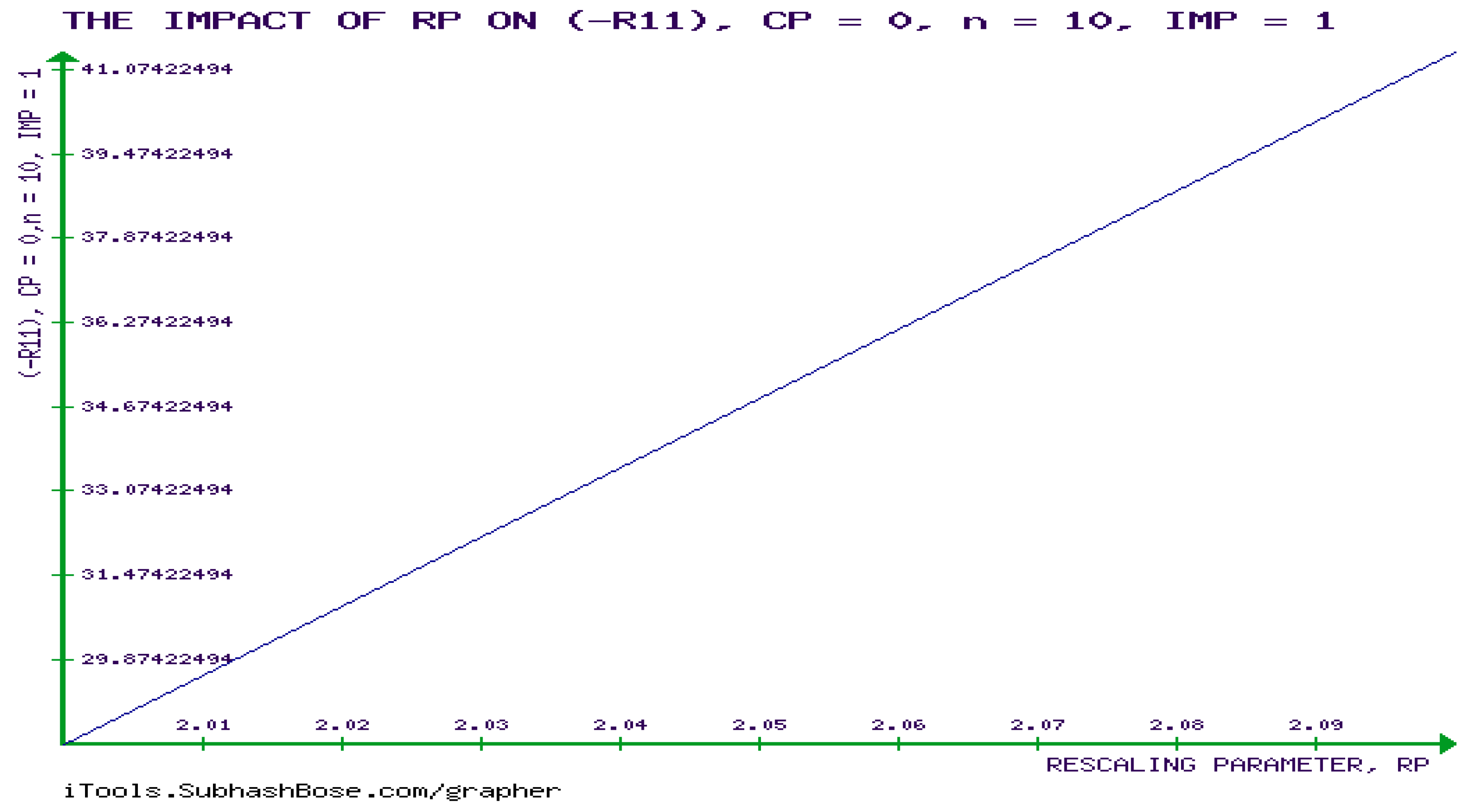
In this section, new results providing under which mathematical requirements, GBM would be developable and has a non-zero 0- Gaussian and Ricci curvatures. Also, a novel sufficient and necessary conditions which characterizes the regions where the surface describing GBM is minimal are determined.
Theorem 6.1 
GBM manifold has:
i) A non-zero 0-Gaussian curvature. ii) A non-zero Ricci tensor. (iii) GBM is developable under the Mong Patch Technique if the condition
ν ψ 1 ν 2 = 4   (6.1)
is satisfied.
(iv) The surface describing GBM is minimal if and only if it holds that
ν = 0   or ν 8 D 0 2 = ( 1 2   l n 2 + 1   2 ψ ( ν 2 ) 1 2 l n ν ) 2 (6.2)
(v) GBM is developable under the Angular Technique for the first principal curvature, K 1 , if the condition
Either ν = 0 o r D 0 = 0 o r
D 0 2 ( 1 ( 5 ν ψ 1 ν 2 ) ) 2 = ( D 0 2 ψ 1 ν 2 4 D 0 2 ν 2 )   ( ( 5 ν ψ 1 ν 2 ) ) + D 0 2 ψ 1 ν 2 4 D 0 2 (6.3)
are satisfied
Proof 
Case i), by definition (2.10), part i), it is enough to show that the α Gaussian curvature
K α = R 1212 ( α ) d e t g i j 0 (6.4)
To this end, the   R i j k l ( α ) can be expressed by
  R i j k l ( α ) = j Γ i k s α i Γ j k s α g s l + Γ j t , l α Γ i k t α Γ i t , l α Γ j k t α ,   i , j , k , l , s , t = 1,2 , 3 , . , n   (6.5)
where Γ i j k α = Γ i j , s α g s k , i, j, k, s = 1, 2, ..., n.
In particular,
  R 1212 ( α ) = 2 Γ 11 1 α + Γ 11 2 α 1 ( Γ 21 1 α + Γ 21 2 α ) ( g 12 + g 22 ) + Γ 21,2   α Γ 11 1 α + Γ 22,2   α Γ 11 2 α ) ( Γ 11,2   α Γ 21 1 α + Γ 12,2   α Γ 21 2 α (6.6)
Following some lengthy calculations, it could be verified that we obtain a family of families of α Gaussian curvatures determined by
  R 1212 α = [ ( D 0 ν ) ( 1 α ) 4 D 0 2 ( ν ψ 1 ν 2 5 ) 2 1 2 D 0 ψ 1 ν 2 + ν 2 ψ 2 ν 2 + ν ψ 1 ν 2 5 1 ν 2 ν 2 ψ 2 ν 2 + 1 ν 1 4 ψ 1 ν 2 ψ 1 ν 2 + ν 2 ψ 2 ν 2 + ( ( 1 α ) 2 64 Δ D 0 4 ) ( ( ν 2 D 0 ) ( 1 ν 2 + 1 8 ψ 2 ν 2 ) + ( 1 ν 1 4 ψ 1 ν 2 ) ) ] (6.7)
Here, a numerical experiment will indicate the required result without any loss of generality due to the higher complexity of calculations.
We have   K ( 0 ) = R 1212 ( 0 ) d e t g i j = 1 Δ ( [ ( D 0 ν ) 4 D 0 2 ( ν ψ 1 ν 2 5 ) 2 1 2 D 0 ψ 1 ν 2 + ν 2 ψ 2 ν 2 + ν ψ 1 ν 2 5 1 ν 2 ν 2 ψ 2 ν 2 + 1 ν 1 4 ψ 1 ν 2 ψ 1 ν 2 + ν 2 ψ 2 ν 2 + ( 1 64 Δ D 0 4 ) ( ( ν 2 D 0 ) ( 1 ν 2 + 1 8 ψ 2 ν 2 ) + ( 1 ν 1 4 ψ 1 ν 2 ) ) ] ) (6.8)
For D 0   = 1 ,   we obtain the following family of zero-Gaussian curvatures devised by
K ( D 0   = 1 ) ( 0 ) = 1 ( Δ ( D 0   = 1 ) ) 2 ( [ ( 1 ν ) 4 ( ν ψ 1 ν 2 5 ) 2 1 2 ψ 1 ν 2 + ν 2 ψ 2 ν 2 + ν ψ 1 ν 2 5 1 ν 2 ν 2 ψ 2 ν 2 + 1 ν 1 4 ψ 1 ν 2 ψ 1 ν 2 + ν 2 ψ 2 ν 2 + ( 1 64 ) ( ( ν 2 ) ( 1 ν 2 + 1 8 ψ 2 ν 2 ) + ( 1 ν 1 4 ψ 1 ν 2 ) ) ] ) (6.9)
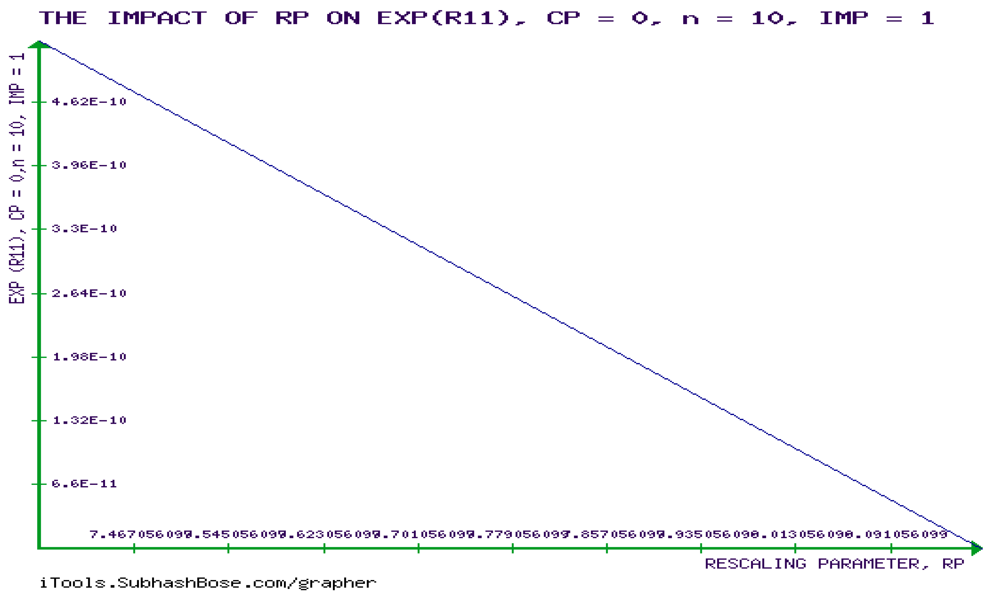
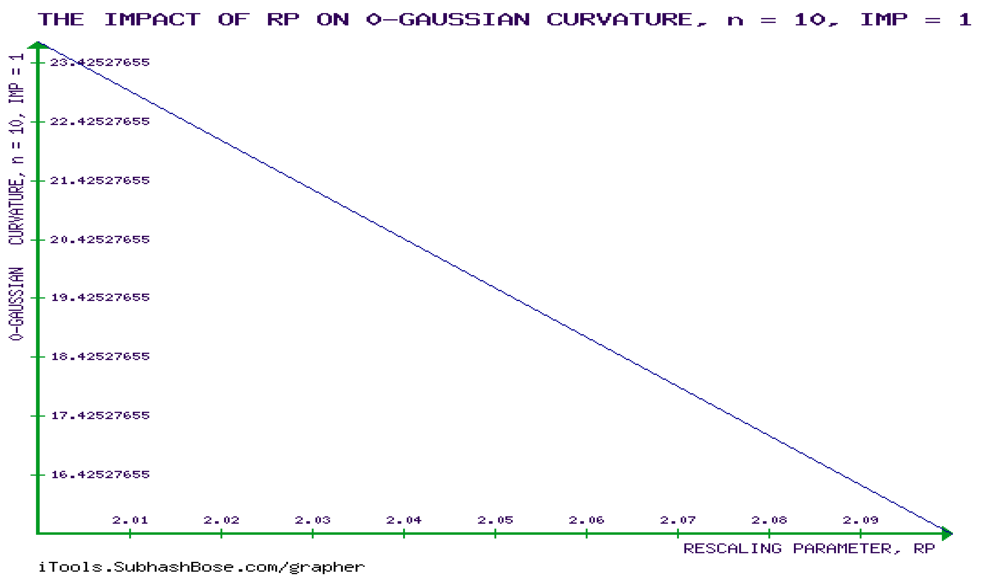
Figure 19. How (RP), namely ν impacts the 0-Gausian curvature for IMP = D 0 = 1 ,   n = 10 .
Preprints 97255 g019
Hence, K α = R 1212 ( α ) d e t g i j i s n o n z e r o .
Case ii)To prove that R i k ( α ) is non-zero of Eqn(2.12)
We need to show that at least one component is a non-zero. Following (6.1), it can be verified that   R 11 ( 0 ) is expressed by:
R 11 ( 0 ) = 4 D 0 ( ν ψ 1 ν 2 5 )   [ 1 4 ψ 1 ν 2 1 4 D 0 1 ν ψ 1 ν 2 + ν 2 ψ 2 ν 2 D 0 ν ψ 1 ν 2 5 2 + 1 ν 2 + 1 8 ψ 2 ν 2 ψ 2 ν 2 + 8 ν 2 1 D 0 2 ν ψ 1 ν 2 5 + 4 ν ν ψ 1 ν 2 5 D 0 ν 4 D 0 2 ν ψ 1 ν 2 5 2 1 2 D 0 ψ 1 ν 2 + ν 2 ψ 2 ν 2 + ν ψ 1 ν 2 5 1 ν 2 ν 2 ψ 2 ν 2 + 1 ν 1 4 ψ 1 ν 2 ψ 1 ν 2 + ν 2 ψ 2 ν 2 + 4 ( ν 2 D 0 ( 1 ν 2 + 1 8 ψ 2 ν 2 + 1 ν 1 4 ψ 1 ν 2 ) D 0 2 ν ψ 1 ν 2 5 (6.10)
The devised value of R 11 0 corresponding to D 0   = 1 ,
R 11 ( 0 ) = 4 ( ν ψ 1 ν 2 5 ) [ 1 4 ψ 1 ν 2 1 4 1 ν ψ 1 ν 2 + ν 2 ψ 2 ν 2 ν ψ 1 ν 2 5 2 + 1 ν 2 + 1 8 ψ 2 ν 2 ψ 2 ν 2 + 8 ν 2 1 ν ψ 1 ν 2 5 + 4 ν ν ψ 1 ν 2 5 1 ν 4 ν ψ 1 ν 2 5 2 1 2 ψ 1 ν 2 + ν 2 ψ 2 ν 2 + ν ψ 1 ν 2 5 1 ν 2 ν 2 ψ 2 ν 2 + 1 ν 1 4 ψ 1 ν 2 ψ 1 ν 2 + ν 2 ψ 2 ν 2 + 4 ( ν 2 ( 1 ν 2 + 1 8 ψ 2 ν 2 + 1 ν 1 4 ψ 1 ν 2 ) ν ψ 1 ν 2 5 (6.11)
Figure 20. How ν impacts R 11 ( 0 ) for D 0 = 1 ,   n = 10 .
Preprints 97255 g020
Figure 20. How ν impacts e R 11 ( 0 ) for D 0 = 1 , n = 10 .
Preprints 97255 g021
It is observed that R 11 ( 0 ) is non-zero according to the curve. It would be zero. Whenever
ν ψ 1 ν 2 5   (6.12)
Following (1.13), ψ 1 ν 2 if and only if n   . So, (6.12) holds if and only if n is infinite. Therefore, R 11 ( 0 ) is everywhere non-zero unless n is infinite. This completes the proof.
The remaining components of the Ricci Curvature Tensor could be computed in a similar fashion.
(iii) Following (2.21), K G = L M M 2 E G F 2 , with E = ( f x ) 2 , F = f x y , G = ( f y ) 2 , L = 2 f x 2 , M = f x y , N = 2 f y 2 .
K G = L N M 2 E G F 2 (2.23)
and its Mean Curvature is
H = 1 2 ( L G 2 M F + N E E G F 2 ) (2.24)
with   E = ( f x ) 2 ,   F = f x y ,   G = ( f y ) 2 ,   L = 2 f x 2 ,   M = f x y ,   N = 2 f y 2
Setting, x = ν ,   y = D 0 a n d   f   t o b e t h e p o t e n t i a l f u n c t i o n Φ θ c . f . ,   3.5 .   It is immediate that,
E = ( 1 2   l n 2 + 1   2 ψ ( ν 2 ) 1 2 l n ν ) 2 ,   F = 1 ν + 1 4 ψ 1 ( ν 2 ) ,   G = ( ν 4 D 0 ) 2 ,   L = 1 4 D 0 ,   M = 0 ,   N = ν 4 D 0 2 (6.13)
By (2.23) and (6.13), clearly it follows that:
K G = 2 ( ν ψ 1 ν 2 4 ) ν 2 ( l n 2 3 + ψ ( ν 2 ) ) (6.14)
It can be seen from (6.13) that K G = 0   if and only if ν ψ 1 ν 2 = 4   , which shows (iii).
To prove (iv), it suffices to show that the Mean Curvature H of (2.24) is zero, if and only if
ν = 0   or ν 8 D 0 2 = ( 1 2   l n 2 + 1   2 ψ ( ν 2 ) 1 2 l n ν ) 2 (c.f., (6.2))
After some lengthy calculations, it could be verified that
H = ν 4 D 0 ( ν 8 D 0 2 ( 1 2   l n 2 + 1   2 ψ ( ν 2 ) 1 2 l n ν ) 2 ) ( ( 1 2   l n 2 + 1   2 ψ ( ν 2 ) 1 2 l n ν ) 2 ν 4 D 0 2 1 ν + 1 4 ψ 1 ν 2 2 ) (6.15)
Clearly, (iv) follows from (6.15).
(v) we have K 1 = B 11 ( 1 + ( f ν ' ) 2 ) 3 2 , K 2 = B 22 ( 1 + ( f D 0 ' ) 2 ) 3 2 (c.f.,(2.27)), f   t o b e t h e p o t e n t i a l f u n c t i o n Φ θ c . f . ,   3.5 .  
After some manipulation, it could be verified that
f ν ' = 1 2   l n 2 + 1   2 ψ ν 2 1 2 l n ν   c o s + ( ν 4 D 0 ) s i n (6.16)
f D 0 ' = 1 2   l n 2 + 1   2 ψ ν 2 1 2 l n ν   s i n ( ν 4 D 0 ) c o s (6.17)
B 11 = 1 ν + 1 4 ψ 1 ν 2 c o s 2 + s i n c o s 2 D 0 + s i n 2 4 D 0 2 (6.18)
B 22 = 1 ν + 1 4 ψ 1 ν 2 s i n 2 s i n c o s 2 D 0 + c o s 2 4 D 0 2 (6.19)
We also have, t a n 2 = 2 ( 2 f ν D 0 ) ( 2 f ν 2 2 f D 0 2 ) (c.f., (2.32)). This directly implies that,
2 t a n 1 t a n 2 = t a n 2 = 2 ν D 0 ( D 0 2 ψ 1 ν 2 4 D 0 2 ν 2 ) (6.20)
The developability of GBM is satisfied if and only if K G = 0   or if either K 1 = 0   o r   K 2 = 0 . Choosing K 1 = 0 . Consequently, B 11 = 0 .   Clearly, it follows that:
t a n 2 + 2 D 0 ν   t a n = 4 D 0 2 ν 2 1 ν 4 ψ 1 ν 2 (6.21)
Hence, t a n = D 0 ν (1 ( 5 ν ψ 1 ν 2 ) ) (6.22). thus, it is obtained by linking (6.20) and (6.21), that
2 D 0 ν ( 1 ( 5 ν ψ 1 ν 2 ) ) 1 ( D 0 ν ( 1 ( 5 ν ψ 1 ν 2 ) ) ) 2 = 2 ν D 0 ( D 0 2 ψ 1 ν 2 4 D 0 2 ν 2 ) (6.23)
(6.23) implies = 0   , o r D 0 = 0 , or 1 ( D 0 2 ψ 1 ν 2 4 D 0 2 ν 2 ) = ( 1 ( 5 ν ψ 1 ν 2 ) ) D 0 2 ( 1 ( 5 ν ψ 1 ν 2 ) ) 2 ν 2 (6.24).
1 ( D 0 2 ψ 1 ν 2 4 D 0 2 ν 2 ) = ( 1 ( 5 ν ψ 1 ν 2 ) ) D 0 2 ( 1 ( 5 ν ψ 1 ν 2 ) ) 2 ν 2 implies
D 0 2 ( 1 ( 5 ν ψ 1 ν 2 ) ) 2 ν 2 = ( D 0 2 ψ 1 ν 2 4 D 0 2 ν 2 )   ( 1 ( 5 ν ψ 1 ν 2 ) ) (6.25)
Thus,
D 0 2 ( 1 ( 5 ν ψ 1 ν 2 ) ) 2 = ( D 0 2 ψ 1 ν 2 4 D 0 2 ν 2 )   ( ( 5 ν ψ 1 ν 2 ) ) + D 0 2 ψ 1 ν 2 4 D 0 2 (6.26)
This completes the proof.

7. The Exponential Matrix of the FIM of GBM ( e F I M G B M Q M )

Theorem 7.1 
e F I M G B M Q M solves d x   d t = Ax.
Proof 
Recalling that GBM’s FIM , g i j reads
[ g i j ] = 1 ν + 1 4 ψ 1 ( ν 2 ) 1 4 D 0 1 4 D 0 ν 4 D 0 2   (7.1)
Rewriting   [ g i j ] in a simpler form,
[ g i j ] = a b b   c ,   a = 1 ν + 1 4 ψ 1 ν 2 ,   b = 1 4 D 0   ,   c = ν 4 D 0 2   (7.2)
If Φ δ = δ = det [ g i j ] δ I = d e t a δ b b c δ = 0 , then δ 2 a + c δ + ( a c b 2 ) = 0.
Therefore,
δ 1,2 = a + c ± ( a 2 + c 2 + 4 b 2 2 a c ) 2
Hence
D = δ 1   0 0     δ 2   ,   e D = e δ 1   0 0   e   δ 2   (7.3)
For δ 1,2 = a + c ± ( a 2 + c 2 + 4 b 2 2 a c ) 2 , the corresponding eigen vectors are 1 ( δ 1 a ) b . , 1 ( δ 2 a ) b . C l e a r l y , follows that the matrix
T = 1 1 ( δ 1 a ) b ( δ 2 a ) b   (7.4)
Thus, e F I M G B M Q M reads:
e F I M G B M   Q M   = T e D T 1 = 1 det T 1 1 ( δ 1 a ) b ( δ 2 a ) b e δ 1   0 0   e   δ 2 ( δ 1 a ) b 1 ( a δ 2 ) b 1 (7.5)
det T = ( a c ) 2 + 4 b 2 0
By (7.5), the required statement is obtained.

8. Conclusions and Future Work

From the perspective of IG, GBM is described, and KD and J-D, the GEs, were established. Additionally, the GBM's matrix exponential of information is developed. This work creates new avenues for research by establishing connections between queueing theory and a wide range of other mathematical fields, including matrix theory, differential geometry, and information theory. In particular, the addition of geometric ties between queueing theory and information allows one to revealing a ground-breaking unified relativistic and of Riemannian geometric analysis of queue manifolds [3,4,7]. This paper's contributions suggest several potential study directions for the new applications of information geometry, such as using information geometrics on different statistical manifolds to further advance many existing physical phenomena.

Appendix A

The following material [72,73,74] as it is needed to carry out mathematical analysis.
Rung-Kutta Method of Order 4
Having the simultaneous equations,
d y d x = F ( x , y , u ) (A.1) , d u d x = G ( x , y , u ) (A.2)
where y and u are prescribed when x = x 0 .   In particular, the Rung-Kutta Method of order 4, generalizes the numerical solutions of (A.1) as follows:
y n + 1 = y n + 1 6 k 0 + 2 k 1 + 2 k 2 + k 3 + O h 5 (A.3)
u n + 1 = u n + 1 6 m 0 + 2 m 1 + 2 m 2 + m 3 + O ( h 5 ) (A.4)
with   k 0 = h F x n , y n , u n ,   ( A . 5 )
  k 1 = h F x n + 1 2 h , y n + 1 2   k 0 , u n + 1 2   m 0   , A . 6 k 2 = h F x n + 1 2 h , y n + 1 2   k 1 , u n + 1 2   m 1   , A . 7
  k 3 = h F x n + h , y n + k 2 , u n +   m 2 ,   ( A . 8 )   m 0 = h G x n , y n , u n , A . 9 m 1 = h G x n + 1 2 h , y n + 1 2   k 0 , u n + 1 2   m 0 ,   A . 10
m 2 = h G x n + 1 2 h , y n + 1 2   k 1 , u n + 1 2   m 1 , A . 11   m 3 = h G x n + h , y n +   k 2 , u n +   m 2 ,   ( A . 12 )
In particular, when F = u , so that (A.1) and (A.2) are equivalent to
d 2 y d x 2 = G x , y , d y d x ,   u = d y d x (A.13)
After some manipulation, it is implied that
y n + 1 = y n + h y n ' + h 6 m 0 + m 1 + m 2 + O ( h 5 ) (A.14)
y n + 1 ' = y n ' + 1 6 m 0 + 2 m 1 + 2 m 2 + m 3 + O ( h 5 ) (A.15)
with   m 0 = h G x n , y n , y n ' ,   6.17   m 1 = h G x n + 1 2 h , y n + 1 2 h y n ' , y n ' + 1 2   m 0 ,   ( A . 18 )
  m 2 = h G x n + 1 2 h , y n + 1 2 h y n ' + 1 4   h   m 0 , y n ' + 1 2   m 1 ,   A . 19   m 3 = h G x n + h , y n + h y n ' + 1 2   h m 1   , y n ' +   m 2 ,   ( A . 20 )
The use of this formula is clearly simplified in those cases when G is independent of y n ' .
Thus, the local truncation[74]error (the error induced for each successive stage of the iterated algorithm) will behave like Error = C h 5 for some constant C. Here C is a number independent of h, but dependent on x 0 and the fourth derivative of the exact solution) at x 0 (the constant factor in the error term corresponding to truncating the Taylor series for y ( x 0 + h ) about x 0 at order h 4 .

References

  1. Nielsen, F. (2020). An elementary introduction to information geometry. Entropy, 22(10), 1100.
  2. Z. Škoda. 2019. Available online at https://ncatlab.
  3. Sommer, S. , Fletcher, T., & Pennec, X. (2020). Introduction to differential and Riemannian geometry. In Riemannian Geometric Statistics in Medical Image Analysis (pp. 3-37). Academic Press.
  4. Mageed, I. A. , Zhou, Y., Liu, Y., & Zhang, Q. (2023, August). Towards a Revolutionary Info-Geometric Control Theory with Potential Applications of Fokker Planck Kolmogorov (FPK) Equation to System Control, Modelling and Simulation. In 2023 28th International Conference on Automation and Computing (ICAC) (pp. 1-6). IEEE.
  5. Mageed, I. A. , & Kouvatsos, D. D. (2019, December). Information Geometric Structure of Stable M/G/1 Queue Manifold and its Matrix Exponential. In 35th UK Performance Engineering Workshop (p. 116). 16 December.
  6. Yarotsky, D. (2022). Universal approximations of invariant maps by neural networks. Constructive Approximation, 55(1), 407-474.
  7. Norton, J.D. , non-Euclidean geometry and curved spaces, department of history and philosophy of science, University of Pittsburgh. 2020. Available online at https://www.pitt.edu/~jdnorton/teaching/HPS_0410/chapters/non_Euclid_curved/index.
  8. Moylan, P. (2023). Poincare and Einstein on Mass-Energy Equivalence: A Modern Perspective on their 1900 and 1905 Papers. arXiv:2305.11852.
  9. Mageed, I. A. , Yin, X., Liu, Y., & Zhang, Q. (2023, August). Z ( a , b ) of the Stable Five-Dimensional M/G/1 Queue Manifold Formalism's Info-Geometric Structure with Potential Info-Geometric Applications to Human Computer Collaborations and Digital Twins. In 2023 28th International Conference on Automation and Computing (ICAC) (pp. 1-6). IEEE.
  10. Mageed, I. A. (2023, July). Rényi’s Maximum Entropy Formalism of Heavy-Tailed Queues with Hurst Exponent Heuristic Mean Queue Length Combined With Potential Applications of Hurst Exponent to Engineering. In 39th Annual UK Performance Engineering Workshop (p. 21).
  11. Bellani, S. , Martín-García, B., Oropesa-Nuñez, R., Romano, V., Najafi, L., Demirci, C.,... & Bonaccorso, F. (2019). “Ion sliding” on graphene: a novel concept to boost supercapacitor performance. Nanoscale Horizons, 4(5), 1077-1091.
  12. Mageed, I. A. , & Zhang, K. Q. (2022). Information Geometry? Exercises de Styles. electronic Journal of Computer Science and Information Technology, 8(1), 9-14.
  13. Mageed, I. A. Cosistency Axioms of Choice for Ismail’s Entropy Formalism (IEF) Combined with Information-Theoretic (IT) Applications to advance 6G Networks. European Journal of Technique (EJT), 13(2), 207-213, 2023.
  14. Levernier, N. , Textor, J., Bénichou, O., & Voituriez, R. (2020). Inverse square Lévy walks are not optimal search strategies for d ≥ 2. Physical review letters, 124(8), 080601.
  15. Stella, A. L. , Chechkin, A. ( 107(5), 054118. [PubMed]
  16. Sakamoto, Y. , & Sakaue, T. (2023). First passage time statistics of non-Markovian random walker: Dynamical response approach. Physical Review Research, 5(4), 043148.
  17. Kouvatsos, D. D. , Mageed, I. A., Anisimov, V., & Limnios, N. (2021). Non-Extensive Maximum Entropy Formalisms and Inductive Inferences of Stable M/G/1 Queue with Heavy Tails. Advanced Trends in Queueing Theory, 2.
  18. Mageed, I. A. Info-Geometric analysis of the dynamics of Fully Automated Evaluation of Coronavirus Disease (FACD) Progression with COVID-19 Cough Sounds Using Minimal Phase Information. FOLS PGR conference, University of Bradford, 2023.
  19. Bhat, A. H. , Siddiqui, N. A., Mageed, I. A., Alkhazaleh, S., Das, V. R., & Baig, M. A. K. (2023). Generalization of Renyi’s Entropy and its Application in Source Coding. Appl. Math, 17(5), 941-948.
  20. Mageed, I. A. , & Zhang, Q. (2022, September). An Introductory Survey of Entropy Applications to Information Theory, Queuing Theory, Engineering, Computer Science, and Statistical Mechanics. In 2022 27th International Conference on Automation and Computing (ICAC) (pp. 1-6). IEEE.
  21. Xu, W. , Liang, Y., Cushman, J. H., & Chen, W. (2020). Ultrafast dynamics modeling via fractional Brownian motion run with Mittag-Leffler clock in porous media. International Journal of Heat and Mass Transfer, 151, 119402.
  22. Mageed, I. A. (2023, July). Where the mighty trio meet: Information Theory (IT), Pathway Model Theory (PMT) and Queueing Theory (QT). In 39th Annual UK Performance Engineering Workshop (p. 8).
  23. Kındap, Y. , & Godsill, S. (2022). Non-Gaussian Process Regression. arXiv:2209.03117.
  24. Mageed, I. A. , & Bhat, A. H. (2022). Generalized Z-Entropy (Gze) and Fractal Dimensions. Appl. Math, 16(5), 829-834.
  25. Mageed, I. A. (2023, July). The Threshold Theorems of Generalized Z-entropy (GZE) fractal dimension (FD) Combined with Influential Applications of FD to Biotechnology Engineering. In 39th Annual UK Performance Engineering Workshop (p. 26).
  26. Mageed, I. A. , & Zhang, Q. (2023). Formalism of the Rényian Maximum Entropy (RMF) of the Stable M/G/1 queue with Geometric Mean (GeoM) and Shifted Geometric Mean (SGeoM) Constraints with Potential GeoM Applications to Wireless Sensor Networks (WSNs). electronic Journal of Computer Science and Information Technology, 9(1), 31-40.
  27. Mageed, I. A. (2023, July). The Threshold Theorems of Generalized Z-entropy (GZE) fractal dimension (FD) Combined with Influential Applications of FD to Biotechnology Engineering. In 39th Annual UK Performance Engineering Workshop (p. 26).
  28. Mageed, I. A. , & Zhang, Q. (2022, September). Inductive Inferences of Z-Entropy Formalism (ZEF) Stable M/G/1 Queue with Heavy Tails. In 2022 27th International Conference on Automation and Computing (ICAC) (pp. 1-6). IEEE.
  29. Mageed, I. A. , & Zhang, Q. (2023). Threshold Theorems for the Tsallisian and Rényian (TR) Cumulative Distribution Functions (CDFs) of the Heavy-Tailed Stable M/G/1 Queue with Tsallisian and Rényian Entropic Applications to Satellite Images (SIs). electronic Journal of Computer Science and Information Technology, 9(1), 41-47.
  30. Mageed, I. A. , Yilmaz, M., Zhang, Q., Celikel, R., & Sidhu, M. S. (2022, October). A review of potential applications of Tensor Decompositions to Electromagnetics and energy works. In 2022 Global Energy Conference (GEC) (pp. 385-390). IEEE.
  31. Dos Santos, M. A. , Nobre, F. M. ( 107(1), 014132.
  32. Yang, X. , Luo, M. M. ( 103(5), 052423.
  33. Mageed, I. A. , Zhang, Q., & Modu, B. (2023). The Linearity Theorem of Rényian and Tsallisian Maximum Entropy Solutions of The Heavy-Tailed Stable M/G/1 Queueing System entailed with Potential Queueing-Theoretic Applications to Cloud Computing and IoT. electronic Journal of Computer Science and Information Technology, 9(1), 15-23.
  34. Mageed, I. A. (2023). The Entropian Threshold Theorems for the Steady State Probabilities of the Stable M/G/1 Queue with Heavy Tails with Applications of Probability Density Functions to 6G Networks. electronic Journal of Computer Science and Information Technology, 9(1), 24-30.
  35. Jena, S. , & Gupta, R. (2020). A unified formalism to study transverse momentum spectra in heavy-ion collision. Physics Letters B, 807, 135551.
  36. Mageed, I. A. , & Zhang, Q. (2022, October). An Information Theoretic Unified Global Theory For a Stable M/G/1 Queue With Potential Maximum Entropy Applications to Energy Works. In 2022 Global Energy Conference (GEC) (pp. 300-305). IEEE.
  37. Mageed, I. A. , & Zhang, Q. (2023). The Rényian-Tsallisian Formalisms of the Stable M/G/1 Queue with Heavy Tails Entropian Threshold Theorems for the Squared Coefficient of Variation. electronic Journal of Computer Science and Information Technology, 9(1), 7-14.
  38. Mageed, I. A. , Zhang, Q., Kouvatsos, D. D., & Shah, N. (2022, October). M/G/1 queue with Balking Shannonian Maximum Entropy Closed Form Expression with Some Potential Queueing Applications to Energy. In 2022 Global Energy Conference (GEC) (pp. 105-110). IEEE.
  39. Mageed, I. A. , & Zhang, Q. (2023). The Rényian-Tsallisian Formalisms of the Stable M/G/1 Queue with Heavy Tails Entropian Threshold Theorems for the Squared Coefficient of Variation. electronic Journal of Computer Science and Information Technology, 9(1), 7-14.
  40. Kumbhakar, M. , & Tsai, C. W. (2022). A probabilistic model on streamwise velocity profile in open channels using Tsallis relative entropy theory. Chaos, Solitons & Fractals, 165, 112825.
  41. Swendsen, R. (2020). An introduction to statistical mechanics and thermodynamics. Oxford University Press, USA.
  42. Hahs-Vaughn, D. L. , & Lomax, R. G. (2020). An introduction to statistical concepts. Routledge.
  43. Kennedy, I. R. , & Hodzic, M. ( 4(2), 729–751.
  44. Spiechowicz, J. , Marchenko, I. G., Hänggi, P., & Łuczka, J. (2022). Diffusion coefficient of a Brownian particle in equilibrium and nonequilibrium: Einstein model and beyond. Entropy, 25(1), 42.
  45. Nkemnole, B. , & Abass, O. (2019). Estimation of geometric Brownian motion model with at-distribution–based particle filter. Journal of Economic and Financial Sciences, 12(1), 1-9.
  46. Erraoui, M. , Y. (2022, November). Images of fractional Brownian motion with deterministic drift: Positive Lebesgue measure and non-empty interior. In Mathematical Proceedings of the Cambridge Philosophical Society (Vol.; pp. 1733693–713.
  47. Aïd, R. , Basei, M., Callegaro, G., Campi, L., & Vargiolu, T. (2020). Nonzero-sum stochastic differential games with impulse controls: a verification theorem with applications. Mathematics of Operations Research, 45(1), 205-232.
  48. Peng, S. (2023). G-Gaussian processes under sublinear expectations and q -Brownian motion in quantum mechanics. Numerical Algebra, Control and Optimization, 13(3&4), 583-603.
  49. Held, P. , Engelkemeier, M., De, S., Barkhofen, S., Sperling, J., & Silberhorn, C. (2022). Driven Gaussian quantum walks. Physical Review A, 105(4), 042210.
  50. Fang, C. , Xu, M., Ma, J., Wang, J., Jin, L., Xu, M., & Li, D. (2020). Large optical anisotropy in two-dimensional perovskite [CH (NH2) 2][C (NH2) 3] PbI4 with corrugated inorganic layers. Nano Letters, 20(4), 2339-2347.
  51. Rao, B. V. (2021). Brownian Motion. Resonance: Journal of Science Education, 26(1).
  52. Yan, X. B. (2021). The physical origin of Schrödinger equation. European Journal of Physics, 42(4), 045402.
  53. Moshayedi, N. (2023). The Path Integral Approach to Quantum Mechanics. In Quantum Field Theory and Functional Integrals: An Introduction to Feynman Path Integrals and the Foundations of Axiomatic Field Theory (pp. 41-87). Singapore: Springer Nature Singapore.
  54. Genthon, A. (2020). The concept of velocity in the history of Brownian motion: From physics to mathematics and back. The European Physical Journal H, 45(1), 49-105.
  55. Ornigotti, L. , & Filip, R. (2021). Uncertainty-induced instantaneous speed and acceleration of a levitated particle. Scientific Reports, 11(1), 18185.
  56. Li, Y. , & Duan, J. (2022). Extracting governing laws from sample path data of non-Gaussian stochastic dynamical systems. Journal of Statistical Physics, 186(2), 30.
  57. NIST, National Institute of Standards and Technology, Digamma functions, 2020. [Online] Available on: https://dlmf.nist.gov/search/search?
  58. Wolfram Mathsworld, Trigamma Functions, Created, developed, and nurtured by Eric Weisstein at Wolfram Research, Last updated: Tue Oct 13 2020. [Online] Available on: https://mathworld.wolfram.com/TrigammaFunction.
  59. Mageed, I. A. , & Kouvatsos, D. D. (2021, February). The Impact of Information Geometry on the Analysis of the Stable M/G/1 Queue Manifold. In ICORES (pp. 153-160).
  60. Nielsen, F. (2021). Progress in Information Geometry. Springer Nature, Switzerland.
  61. Chow, B. , Lu, P., & Ni, L. (2023). Hamilton’s Ricci flow (Vol. 77). American Mathematical Society, Science Press.
  62. Ferreiro Subrido, M. (2023). Conformal structures and solitons in pseudo-Riemannian geometry. 2023. [Google Scholar]
  63. Gorard, J. (2020). Some relativistic and gravitational properties of the wolfram model. arXiv:2004.14810.
  64. Sun, A. (2020). Compactness of constant mean curvature surfaces in a three-manifold with positive Ricci curvature. Pacific Journal of Mathematics, 305(2), 735-756.
  65. Partner, A. , & Vernitski, A. (2023). Maths lecturers in denial about their own maths practice? A case of teaching matrix operations to undergraduate students. MSOR Connections, 21(3).
  66. Binninger, A. , Verhoeven, F., Herholz, P., & Sorkine-Hornung, O. (2021, August). Developable approximation via Gauss image thinning. In Computer Graphics Forum (Vol. 40, No. 5, pp. 289-300).
  67. Jia, Y. B. (2020). Gaussian and mean curvatures. Com S, 477(577), 1-7.
  68. Li, Q. R. , Sheng, W., & Wang, X. J. (2020). Flow by Gauss curvature to the Aleksandrov and dual Minkowski problems. Journal of the European Mathematical Society (EMS Publishing), 22(3).
  69. Cao, L. , Yao, Y. ( 104(5), 1143–1166.
  70. Vaccaro, J. , & Lipnikov, K. ( 61(5), 2285–2304.
  71. Leader, J. J. (2022). Numerical analysis and scientific computation. CRC Press.
  72. Luan, V. T. (2021). Efficient exponential Runge–Kutta methods of high order: construction and implementation. BIT Numerical Mathematics, 61(2), 535-560.
  73. Faissole, F. (2024). Formally-Verified Round-Off Error Analysis of Runge–Kutta Methods. Journal of Automated Reasoning, 68(1), 1.
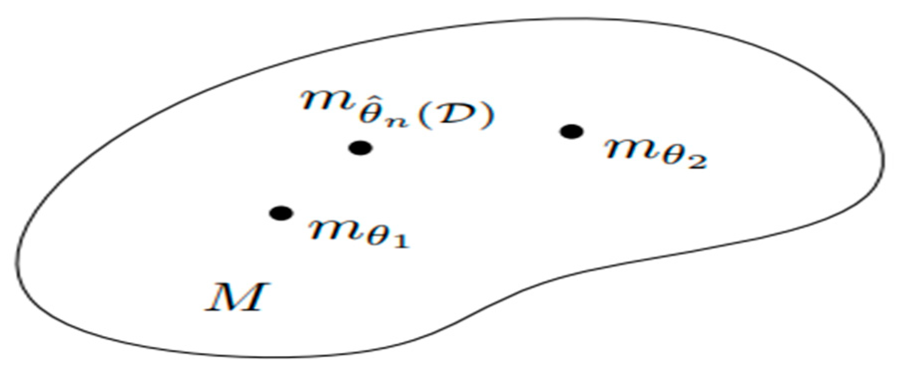
Figure 1. SM’s parametrization [1].
Preprints 97255 g001
Figure 2. Geodesics on curved surfaces geometric representation (c.f., [7]).
Preprints 97255 g002
Figure 4. (c.f., [57]).
Preprints 97255 g004
Figure 7. The elliptic paraboloids z = x 2 + 2 y 2 ( to the left ) and z = x 2 2 y 2 ( to the right ) (c.f., [68).
Preprints 97255 g007
Figure 8. (c.f., [68).
Preprints 97255 g008
Figure 9. (c.f., [68).
Preprints 97255 g009
Figure 10. (c.f., [68).
Preprints 97255 g010
Figure 12. NVP is non-zero.
Preprints 97255 g012
Figure 13. the temporal path of the rescaling parameter.
Preprints 97255 g013
Figure 14. The temporal path of the velocity of the rescaling parameter.
Preprints 97255 g014
Figure 17.  
Figure 17.  
Preprints 97255 g017aPreprints 97255 g017b
Figure 18.  
Figure 18.  
Preprints 97255 g018aPreprints 97255 g018b
Disclaimer/Publisher’s Note: The statements, opinions and data contained in all publications are solely those of the individual author(s) and contributor(s) and not of MDPI and/or the editor(s). MDPI and/or the editor(s) disclaim responsibility for any injury to people or property resulting from any ideas, methods, instructions or products referred to in the content.
Copyright: This open access article is published under a Creative Commons CC BY 4.0 license, which permit the free download, distribution, and reuse, provided that the author and preprint are cited in any reuse.
Prerpints.org logo

Preprints.org is a free preprint server supported by MDPI in Basel, Switzerland.

Subscribe

© 2024 MDPI (Basel, Switzerland) unless otherwise stated