Submitted:
17 January 2024
Posted:
18 January 2024
You are already at the latest version
Abstract
The air transport industry has experienced important transformations over the last decades, despite its continuous global trend of growth. After air transport liberalization process, the present market situation depicts a reduced number of large hub & spoke airlines and an important number of so-called low-cost carriers (LCC). One may wonder why airlines that were once thriving and profitable before liberalization have disappeared, some even recently amid an expansion in demand. To answer that question and others related to it, this paper proposes a management model focused on the airline business, putting in relation the main variables defining the business behavior of an airline. The lessons learned from the past, and the solutions gathered from the model related with, will provide a sound basis to address the new challenges for the next years to come, as it is the case of the new environmental regulations focused on the air transport decarbonization.
Keywords:
Airlines
; Air transport liberalization
; Competition
; Management Model
; Environment regulations
; Decarbonization
1. Introduction and Some Literature Review
The basic scope of this research is the air transport industry in the United States and in Europe, but its results and conclusions are applicable to the management of any airline in the world. Most of the data are up to and including the year 2019 to avoid the singularity of the Covid 19 pandemic. In 2022 the air transport industry experienced a recovery, with global figures up to 87% of 2019; for 2023 it is expected to reach 93% of 2019 [1].
Since the liberalization of domestic air traffic in the United States under the US Airline Deregulation Act [2] and the subsequent liberalization in Europe (1987/88–1997), the air transport industry has undergone relevant, profound, and prolonged changes. The demand changed its behavior, with a loss of loyalty and a significant increase driven by a greater accessibility of supply. Not only did the rules of the game change, but so did the playing field. Liberalization marked a very significant watershed in the air transport industry [3,4]. The first important legal measure, the US Airline Deregulation Act, applied immediately and prompted the irruption of Low-Cost Carriers (LCC) as new entrants [5], which drastically changed air transport market.
Not all LCCs entrants had continuity. After initial expansion and success, many LCCs disappeared or were taken over within a few years, proving that offering low fares is a necessary but not sufficient condition for market success [6]. Some traditional carriers also disappeared; of the so-called 'big four' before liberalization, American Airlines, Eastern, TWA and United Airlines, only American and United remain operational.
Unlike in the United States, the liberalization of air transport in the European Union (EU) came about gradually. It began in 1987/88 and ended in 1997 [7,8]. LCCs also emerged as strong new entrants and had a huge impact on the market, competing intensely in short and medium haul traffic with both well-established scheduled and charter airlines.
The LCC approach is a whole action system, not just a set of activities [9,6]. The unit cost of LCCs were much lower than that of established airlines, reflected in their much more efficient break–even curve, which includes the break–even Load Factor (LFbe). The main concern of established airlines was to reduce costs as much and as quick as possible. Moving the break–even curve down was a must for established airlines in their short and medium haul network to match and compete with LCCs, and being able to provide lower fares. The largest increase of traffic in the last years has not been in the traditional segments but in new market ones, with lower fares and stimulated by the LCC entrants, where many established airlines have not been able to adapt [10]. That is why some established airlines created new low–cost subsidiary airlines. An example is that of Iberia and Iberia Express. The new subsidiary airlines are distinct but not distant from the parent airline. This airline within airline (AWA) approach has not always been successful [6]. Another possibility is to change from the parent airline itself, an internal change, if there is leadership capability to persuade and convince about the change.
In the last 10 years, up to and including 2019, scheduled passenger traffic worldwide maintained a sustained and significant level of growth, with an average above 6% per year in terms of Revenue Passenger Kilometer (RPKs) [11]. In the European Union, the average annual passengers’ growth was above 4% [12] and yet, despite this market growth, in recent years some airlines in Europe, both scheduled and charter, have disappeared. The current market share of LCCs worldwide is above 30% of the world total scheduled passengers (37% in Europe as per [12]), with growth around 1.5 times the rate of the world total average passenger’s growth [11]. From September 2022 to August 2023, the LCCs flights, seats and Available Seat Kilometer (ASKs) have increased by 2 percentage points (pp) [13].
There has been a consolidation of the industry around two main business models: full-service network airlines and LCCs. In the case of network airlines, 6 large international airlines have been established, generally known as megacarriers: American Airlines, Delta Airlines and United Airlines in the United States; Air France–KLM Group, International Airlines Group (IAG) and Lufthansa Group in Europe. All of them operating through their hubs. These large airlines have been able to adapt to the new competitive environment and change.
In the case of LCCs, with point-to-point, short and medium haul traffic, Southwest is the hegemonic airline in the United States. Ryanair and easyJet are the two hegemonic ones in Europe. Both are highly cost efficient oriented, but easyJet includes some hybridization [14], with a differentiated and superior product oriented also towards business class.
Following liberalization, the future of the air transport industry has been less and less of an evolutionary consequence of the past, driven by the immediacy of change. For established airlines, the challenge has been (and still is) not just to change, but to change quickly. Established airlines that have failed to do so have either disappeared or been taken over.
Table 1.1 is a set of business data of network, full-service airlines and point-to-point LCCs airlines, corresponding to 2019, well after liberalization (source: Annual Reports of each airline, currency in Euros, €). Table 1.1 includes airlines that successfully survived after the turmoil of air transport liberalization and the highly competitive environment created.
where:
ASK: available seat kilometer
RPK: revenue passenger kilometer
Yield: Revenue per passenger kilometer (unit revenue)
Cost/ask: unit cost per ASK = CASK
Pax: passengers
LF: Load Factor, relationship between rpk and ask (RPK/ASK), in %
LFbe: Load Factor of break–even (when Revenues equal Costs, so Results are zero)
ΔLF (pp): difference between LF and LFbe in percentage points
1.1. Some Interesting Aspects from These above Tables
a) Load Factor and yield: In 1977, just before the application of the US Airline Deregulation Act, the average industry Load Factor (LF) of scheduled legacy carriers was about 62%, with a LFbe around 60%. Today such LF seems extremely low in comparison to those of 2019. The average yield of legacy carriers in 1977, in real terms of 2019, was 11.2 cts/RPK [15]. For legacy carriers, the average decrease of yield has been around 24%, a real benefit for passengers. That is why the current LF is much higher than that of 1977. Nowadays, the LF averages between 82% and above 90% (see Table 1.1). This is a big LF leap in relation to those of before liberalization. These much higher LFs represent a better use of capacity, a better efficiency of air transport; a lower fuel consumption per passenger (that is, a lower carbon emission per passenger), and a lower unit cost per passenger despite some little increment of CASK due to the increment of LF.
b) Unit cost over the years: The average unit cost (CASK) of legacy carriers of 1977, in real terms of 2019, was 6.62 cts/ASK [15], which is similar to the present ones. That means the unit cost over the years is being pretty much constant in current terms, which means it is much lower in real terms. As an example, Iberia kept a unit cost around 7 cts/ASK during the last 10 years up to 2019 [16,17], and Norwegian around 4 cts/ASK during the same period [18]. Airlines make a permanent effort to keep or even lower their unit cost over the years, as the high actual average LF does not allow but just tight increases, if any. Should the unit cost increase, LFbe would increase and getting closer to the actual average LF, reducing profitability.
c) Other Revenue: this includes no-show passengers and/or other revenue due to some commercial policy, air cargo, selling services to others, etc., plus the ancillary revenue, showing their contribution to total revenue for each airline. The ancillary revenue are extra products not included in the fare that passenger buy, at their choice: food on board, baggage, seat selection, on-board sales, etc. LCCs focus a great deal on ancillary revenues, which are an important part of total revenues [13]. As an example, in the case of Ryanair the ancillary revenue is 35% of its total revenue, with a figure much bigger than profits. Some legacy carriers are also using the break down fare in the same way than LCCs, especially for short flights [13].
d) Differences between the actual LF and the LFbe: such a difference is a point of interest for airlines, which shows the margin to increase revenues without increasing fares. As an example, IAG, Ryanair, Delta and Southwest have a margin between 11pp and 12pp, which provides to them a good margin to increase revenues without increasing fares. On the contrary, Air France-KLM and Lufthansa Group have both little margin (3.6pp) to increase revenues. The alternative to increase revenue by increasing fares is also difficult in a highly competitive market, which sets the fares. The commercial position of Air France-KLM and Lufthansa Group is weaker than that of IAG, Ryanair, Delta and Southwest.
e) Difference of unit cost and yield between Southwest and Ryanair: Southwest has a unit cost and yield higher than those of Ryanair and other competitors in US. Southwest can afford this because of its company culture of being very close to the customer, getting from it its firm loyalty and willing to pay a premium fare for a superior product [19]. In addition, Southwest pays higher salaries. Ryanair is not a clone of Southwest.
f) Financial performance: Table 1.2 shows the financial performance of several airlines and groups in 2019. The Aena (Spanish Airport Authority) financial performance has also been included as a reference of related industry. It might be of interest to notice the different profit margin over revenue of the airlines. It can be seen the high profit margin of Southwest and IAG (13.2% and 8.9%, respectively) in contrast with Air France–KLM and Lufthansa, much lower (1.3% and 4.8%, respectively). The champion is Aena, with a profit margin of 42.2%, tripling the best airline profit margin. In a good demand condition and if well managed, airports use to provide better profitability than airlines. Aena went public on February 2015 and the first closing day its shares rose above 20%. After two years, the Aena stock value multiplied by 2.3.
2. The Purpose of This Paper
The way from air transport liberalization (and its highly competitive new market) to nowadays has been a long and difficult way. Not all the traditional airlines had the ability to adapt to the new competitive environment and many of them disappeared or were absorbed. It can be remembered the case of emblematic airlines like Pan Am, TWA, Eastern and others in the United States, and Swissair, Sabena, Britannia, and others in Europe.
Looking at the big transformation of the air transport industry in the last two decades, the question that raises is how is it possible that airlines, once so robust and solvent, which have managed this business so thrivingly for years, have disappeared even amid an expansion in demand in recent years? Why have they not been able to adapt their expertise to this new competitive environment? It is possible that the immediate cause of bankruptcy or absorptions of some airlines was due to economic and financial problems; to a sudden change in the business environment that they did not know how to foresee and were unable to manage; to the obsolescence of the product for a different type of demand; to the new unaffordable low fares; maybe related to reasons of business consolidation and economies of scale, etc. These and others could be some of the immediate causes. But due to the magnitude of the restructuring, both in the United States and in Europe, there could be other causes linked to the management of the business, linked to its know-how. Linked to the know-how of the strategic break–even curve, and the rationale involved in to be competitive. The purpose of the present work is to investigate this hypothesis, by developing a simple business management model to identify the problems and guide toward the solutions. We may wonder what lessons we can learn from the past to face the challenges of the future.
In this sense, this paper analyzes and studies the variables that define and describe the business behavior of an airline, making possible a quick decision action to keep the airline profitability and competitivity. It becomes a useful tool to face new challenges for the coming years as the application of the new environmental regulations needed to achieve the air transport decarbonization, and its associated cost impact.
3. Methodology: The Management Model
The three fundamental variables that constitute and describe any airline business behavior are:
- Yield: , revenue per revenue passenger kilometer ()
- Unit cost: , cost per available seat kilometer, CASK ()
- Load Factor: (= %)
where,
: Revenue per passenger kilometer
: Available seat kilometer
For any business organization,
where,
: Results
: Revenue
: Cost
For the case of an airline, considering the three fundamental business variables defined above (, , ), we have:
Substituting in
Dividing this equation by :
Substituting the definition of (=) in the above equation we obtain the business general equation of an airline, which determines its economic results :
Equation (1) relates the economic results of an airline with the three fundamental business variables, and the production of . In addition, it provides information on the economic performance of the airline per unit of production in . Figure 3.1 shows the relationship among yield , and Results () for a given unit cost . Any variation of moves the surface back and forth. It is a gentle doubly ruled surface, with smooth slope forward (to increase results, yield or LF or both must increase).
The red line is the locus of the surface with results , whose curve will be shown below. The black lines are the locus of the surface with constant results, either positive or negative. To draw the surface, we have taken as a sample (it will be explained afterwards).
For the management of an airline, it is useful to consider the case where . This allows us to know what combination of variables achieve the break–even of the business, and facilitates the visualization (Figure 3.2) of the basic reference from which to obtain positive results: .
From equation (1), the condition for is .
That is:
Figure 3.2 is the graphic representation of equation (2), corresponding to the red line on the results surface ():
The unit cost has been taken from Aviaco in 1992 [20], a subsidiary airline of Iberia for short and medium haul. This unit cost is similar to that of Iberia for its own short and medium haul at the time [21].
Figure 3.2 is called the break–even curve. For each yield value on the curve, the break-even Load Factor () is obtained. And vice versa. Yield and values on the curve produce zero results: . For pairs of yield and values above the curve, positive results are obtained (); and for yield and values below the curve, negative results are obtained ().
The break-even curve can oscillate continuously due to the permanent variation of the unit cost associated to the variation of the fuel price, €/$ parity, airport landing fees, etc. Consequently, the area of commercial operation should be not only above the curve, but also as far away as possible to avoid negative results due to an unforeseen oscillation that increases the unit cost and swallows the economic results of the airline.
The break-even curve will be used as a management model to understand the fundamental business variables of an airline and the relationship among them. It will serve to identify and graphically visualize the picture of the airline to facilitate decision-making together with its rationale.
4. Results: Application of the Model to the Management of Airlines
4.1. The Break–Even Equation and Its Associated Curve
The break–even equation and its associated curve is a synthesis that brings together the rest of the air transport business equations and can be considered a basic equation and curve for managing the business of an airline.
Its applications can refer to a single route or to a set of routes. By aggregation, the break–even curve of an airline's total network can be obtained.
The break–even curve of a partial set of routes cannot be extrapolated to the entire network or to another set of routes because it might not reflect reality; it may not even be representative but offer a rather misleading image. Likewise, the break-even curve of the total network may not indicate exactly, with due accuracy, the partial behavior of a set of routes. The more disperse the stage length of the network, the less comparable are the partial and total behaviors and vice versa. The unit cost, which defines the position of the break–even curve, varies with the stage length. For a given airline, the unit cost of short and medium haul is higher than that of a long haul one, unless the labor costs (and others) allocated to short and medium haul are much lower than those allocated to long haul. Thus, when some studies [22] state that full-service network airlines are closing the cost gap with respect to LCCs, it is true, but it is a non-homogeneous comparison when mixing long haul stage lengths with short and medium haul ones, and that can lead to incomplete conclusions.
Any comparison among airlines to take decisions must be made in a homogeneous way to be effective, not only in terms of similar network but also in terms of product. For example, the cost structure of LCCs is very different from that of network airlines [19]. We can compare the fuel cost over total operating costs of Ryanair, that is 46% [23], while that of IAG is 29% [24]. The weigh of fuel cost in both airlines is very different. Decisions to be taken must consider the differences. In terms of costs, the patterns for comparison among airlines are productivity of assets (daily airplanes utilization, turnaround time, technology, etc.) and productivity of people. Another reference of comparison may be the difference between the actual LF and the LFbe.
Let us consider an airline A with a unit cost taken from Aviaco in 1992 [20].
And let us also consider an airline C, a new entrant LCC for short and medium haul, with a unit cost much lower than that of A: . This figure corresponds to an average for the short and medium haul of easyJet [25] and Ryanair [26].
Figure 4.1 shows that if the competitor C enters the same route network with a lower break-even curve (lower unit cost), it is immediately observed that airline A has an entire risk area between the two break–even curves.
The risk is that the market of A is transferred to C due to the attractiveness of its lower fares. Market loyalty to A may shift to C, unless other attributes of A's product (service quality, branding, trust, etc.) retain enough loyalty to A to remain in the profit zone. One quick glance of the break-even curve will suffice to see all this information. That information is more than enough to highlight strategic issues and take decisions. If necessary, greater efforts of accuracy can be made [19].
As an example, from Figure 4.1, a yield of means a for airline C and a for airline A, much higher than that of airline C. That requires airline A decrease its to compete in fares with airline C, that is, to move its break–even curve down.
Related with Figure 4.1, it could happen that the strength of the market's loyalty to airline A is such as that by simply reducing fares (lower yield), it would stimulate demand and produce enough increase in to remain in the positive results zone (Figure 4.2). That is, maintaining the airline’s current break–even curve. It is a first approach to change, an initial test.
If this first approach does not work, the airline must change the curve, reduce its unit cost . In this case, the airline A must move its break–even curve down (Figure 4.3) to competitor C’s position, moving in turn the commercial zone CZ (green arrow).
The same concept applies for long-haul. Figure 4.4 represents break–even curves for network (blue) and point-to-point (green) airlines operating short, medium and long haul. The blue one corresponds to a mix of British Airways and Iberia, with unit cost [27,17]. The green one corresponds to Norwegian, whose unit cost is [18]. To consider an airline with just long-haul operation, Virgin Atlantic would be an example: its unit cost is [28]. A guess for Norwegian just long-haul unit cost could be around , since the long-haul unit cost is usually lower than the short and medium haul.
4.2. The Curve Explains the Equation
The break–even curves, graphically and illustratively, provide clarity and promptness of analysis. They define the business behavior of an airline, which is what we could call its Business Performance Indicator (BPI). They are valid equations in normal and exceptional conditions, for all boundary conditions and for all management models, and for all airlines. They allow for the following:
- To visualize where the airline is (and where it should be, if that were the case) on its different routes and markets and, by aggregation, in the total network.
- To visualize where its competitors are and benchmark the behavior of the airline in relation to competitors in a homogeneous way according to routes, markets, etc. This allows to identify areas of risk or, conversely, areas of business strength. The possible decisions to be made may not affect the entire network but just rather the set of routes in competition with other airlines. The change can be selective if route management can be split.
- To visualize the area of yields and where the market is, where business management should be heading.
- To visualize not only where the airline should be, but also where it would like to be, the target vision.
The break–even curve defines the business concept of an airline and provides a clear vision of its business performance.
4.3. The Challenge of Moving the Break–Even Curve Down
Moving the break–even curve down is not an easy task. But it is affordable. The improving change, including LF increase, may involve three patterns of action:
- Cost reduction
- Breaking down the low fares as LCCs do
- Quick implementation
4.3.1. Cost Reduction
Moving the break–even curve to lower positions implies reducing the unit cost. This means a whole structural rethinking of costs at a global level and achieving greater efficiency, a better and more efficient value chain than competitors [20]. Most likely, all of this is not a change within the system but a change of system, maybe breaking molds. It is not a reform, but a transformation. Leadership capability is required to persuade and convince others of the need and virtue of change in an airline, to move the break-even curve down. It is in difficult times when leadership is most needed, most important, and most visible [29]. Also, knowledge of managing change is required [30,31]. All of this is solutions oriented.
Cost reduction may have two ways of action: a) cost reduction of the several cost items and b) increasing productivity of both assets and people.
- a)
-
Airline costs can be splitted in two blocks: Direct Operating Costs (DOCs) and Fixed Operating Costs (FOCs). DOCs include mainly: Fuel, Flight Operations (OPS), salaries, Maintenance, Repair and Overhaul (MRO), Handling, Catering, Landing Fees, Navigation Charges. FOCs include mainly: Labor, Assets depreciation, Infrastructure, Financial, Marketing and Sales, Advertising, Research & Development plus Innovation, Technology, Overheads.Many costs of an airline are a mix of DOCs and FOCs. For example, MRO include fixed labor and equipment plus DOCs as maintenance reserves for airplane and engine overhaul related to airplane’s utilization in Block Hours (BH) and cycles (number of flights). The isolated analysis of each cost can be confusing because of the mix of DOCs and FOCs involved in. The value chain provides the basic tool for cost analysis [19]. Costs by nature (labor, fuel, etc.) or by functions (OPS, MRO, Marketing, etc.) are also of interest to cross check them with value chain costs.DOCs are also related to the operating performance of the airplane (maximum range, long range, etc.). In some cases, they can have opposite effects. For example: fuel consumption increases as speed increases; on the contrary, maintenance costs decrease with speed, as they are related to the BH utilization of the airplane. From that opposite behavior related to speed, the optimum speed for minimum cost combination of fuel and MRO can be obtained.
- b)
- Increasing productivity (efficiency) of both assets and people is crucial. This is a must to work out at the top of efficiency and effectiveness. Fleet utilization, multifunctional activities, flexibility on labor agreements (collective bargain) are essential cost drivers of value chain.
4.3.2. Economy Fares Breakdown
Establish a set of different basic fares according to demand behavior over time, based upon yield management. The goal is to increase LF as much as possible in every flight, with better coupling of supply and demand. In addition, manage ancillary revenues, as LCCs do, with extra products not included in the fare, as already mentioned.
4.3.3. Quick Implementation of Change
To properly face the competitors’ challenge, change must be implemented as quick as possible to avoid or reduce its negative financial impact. Time is tight. The velocity of competition must not be faster than the airline velocity of change.
To successfully address the future challenges of the industry, in addition to the importance of the airline business concept defined, the human factor will continue to be a crucial key factor in providing a good customer experience. The product of the air transport industry is a proximity product.
An example of change can be found in Iberia (network airline). In 2009, Iberia was going through some very difficult and conflictive times, with losses more than €400 million, and its continuity was on the line. However, the airline knew how to reinvent itself and change. Iberia broke molds and took a qualitative leap by solving the conflict and generating momentum. It turned its results around and brought back quality and enthusiasm. During the change process, the employees, spontaneously and voluntarily, wore a heart sticker on their lapel. In 2019 (before the pandemic), Iberia had managed to reduce its unit cost by nearly 22% in real terms, achieving positive results close to €500 million [16, 17]. Iberia managed to make the elephant dance. And it grew back. Iberia incorporated the value of change into its core values.
5. The Impact of New Environmental Regulations
Climate change is a main concern all over the world to preserve the planet. Commercial aviation stakeholders are fully aware of it and to reduce noise and emissions. Investing on technology is a priority at the airline industry, with airplanes, engines and systems state of the art. All aviation stakeholders are committed to reduce carbon emissions for environmental and economic reasons.
The air transport industry began to be concerned first about noise more than 50 years ago. FAR Part 36 (1969) in the United States and ICAO Annex 16 (1971) worldwide enacted the first regulations on noise. Airlines applied several Noise Abatement Procedures (NAP), with cut–back at takeoff and low power–low drag approach at landing. Noise regulations were updated in 1977, 2006 and 2020, increasing the requirements levels.
ICAO began to regulate emissions in 1980 (Annex 16, Vol. II). There are several elements in the emissions with effect on climate change. Most of them, like cirrus cloud formation (contrail), are still with poor level of scientific certainty. The scientific level certainty of Carbon Dioxide (CO2) is good and is where Aviation Regulations Authorities have decided (for the time being) to put their focus on, implementing measures with the target of getting results in the short term.
The stoichiometric (perfect) combustion of 1 kg. of kerosene (the aviation fuel) produces between 3.15 – 3.16 kg. of CO2, depending on fuel specification. The amount of CO2 emissions is proportional to fuel consumption during airplane operations. The ICAO target is to optimize the fuel burned considering three main stakeholders:
- Manufacturers to produce more efficient airplanes, engines and systems.
- Airlines to improve operating procedures and to optimize fleet utilization.
- Infrastructure suppliers: airports to provide capacity enough to avoid congestions and ATC for an optimum air traffic management.
According to IATA experience and ICAO targets, these three actions of ICAO produce a fuel efficiency improvement between 1.5% and 2% per year, which is not enough to compensate the international traffic growth of about 5% per year. With the agreement of the main aviation stakeholders to solve this gap, ICAO added a new action to the three technical ones, introducing economical mechanisms and market incentives to achieve established targets: Market Based Measures (MBM). The whole set is known as ‘The Four Pillar’. The strategy and targets are represented by Figure 5.1, showing the CO2 reduction plan in the next coming years with the target of net carbon zero by 2050 [32].
The MBMs applied so far and updated to December 2023 are: Voluntary Agreements, Taxes, Charges, Emissions Trading System (ETS) and Offsetting (CORSIA).
ETS is being applied in some countries. It is applied to flights between European Economic Area (EEA) States since 2013. ETS is a cap-and-trade system. The Regulatory Authorities establish a cap for participant’s emissions, providing them some allowances to emit at no cost. Participants can buy and sell emissions allowances in the open carbon market to balance the free allowance quantity with their actual emissions. Participants include airlines and industrial plants, because air transport alone would be a net buyer for ever since its annual traffic growth is greater than its fuel efficiency increase per year. The allowance price has increased sharply since 2020 (Figure 5.2). The EU announced to eliminate free allowances by 2027, in whose case the price per liter of kerosene might increase about 0.25 €, a third of the present price. The ETS system gives biofuels a zero-emission factor, biofuel is practically exempted of the emissions market.
The EU proposed to ICAO the application of a worldwide ETS for international flights, but the proposal was rejected by most States (2007 ICAO General Assembly).
Because of this rejection and trying to reach a general consensus, ICAO proposed a new MBM named CORSIA (Carbon Offsetting and Reduction Scheme for International Aviation), approved in October 2016. The target is to offset the excess of CO2 emissions above the 2019 level. Above this base line, a cost is applied to airlines from countries subject to payment. It is expected that about 90% of international flights in 2027 will be CORSIA included. The period of 2021-2023 is a pilot period and CORSIA system will be fully operative in 2024-2026 for participants. As of 2027 will be mandatory for the rest of States with high international traffic operation. At present, 125 States have announced their participation, starting in 2024.
All of this is consistent with the application of Voluntary Agreements, Fuel Taxes and Charges, to be applicable subject to decision of each State or airline, depending on the case.
5.1. UE SAF Mandatory Blending
There is a consensus to introduce Sustainable Aviation Fuel (SAF) as the main factor to eliminate carbon emissions in the short and medium term. The EU’s ‘Fit for 55’ climate package (July 14, 2021) included a proposal of minimum mandatory blending of SAF to fuel suppliers at EU airports and was approved in September 2023. The obligation also includes a minimum percentage of e-kerosene (the aviation category of e-fuels). The package involves aviation fuel suppliers, airlines and airports. The proposal considers e-fuel has the highest potential for decarbonization; hence to push e-fuel introduction into the market. The plan to accomplish this with a minimum blend of SAF and e-kerosene is [34]:
- 2% from 2025
- 6% from 2030, with a minimum of 0.7% e-kerosene
- 20% from 2035, with a minimum of 5% e-kerosene
- 34% from 2040, with a minimum of 8% e-kerosene
- 42% by 2045, with a minimum of 11% e-kerosene
- 70% by 2050, with a minimum of 28% e-kerosene
The regulation of SAF blending would be flexible to adapt within the first 5 years of application. The target is that a minimum of 95% departures from EU airports will be covered.
After a successful Virgin Atlantic Boeing 747/400 first commercial flight with a mix of 80% of conventional kerosene and a 20% first generation biofuel, more than 40 airlines have tested different aviation biofuels with satisfactory results. The properties of kerosene did not change at all by blending biofuel, known by drop-in fuel. The US American Society for Testing and Materials (ASTM International) approved a biofuel specification (July 2011) and most of today in service engines can operate up to a mix of 50% of such a biofuel in the standard kerosene. EU accepted the challenge to promote biofuels on air transport, whose methods were established in SET (Strategic Energy Technology) Plan.
Present technology can provide Sustainable Aviation Fuels (SAF) with reduced carbon emissions, measured in a Life Cycle Basis, to substitute standard kerosene. What is not so clear is if can be done in a cost-effective way: this is a real challenge. According to recent EU estimation, biofuel might cost above 2,000 €/ton vs 700 €/ton of standard kerosene at today’s prices (around 3 times), which may be unaffordable for the air transport industry. However, it is expected the price will get down as learning curve improves and production scales increases.
5.2. Position of the Industry
In a press release of July 14, 2021, related to EU’s ‘Fit for 55 package’, IATA stated that SAF is the most practical solution but is concerned about cost. ACI Europe (airports) is a supporter of the EU blending mandate, with airports fully compatible with SAF use. Aviation industry is committed to decarbonization but opposed to taxes as a solution for change. To reduce emissions, IATA claims for a constructive policy to focus on production incentive for SAF and delivering a Single European Sky. IATA has proposed a more ambitious target, with net-zero carbon emission by 2050. The 41st ICAO Assembly (September/October 2022) agreed also with the goal of net-carbon emissions for international aviation by 2050 in support for UNFCCC Paris Agreement. In 2020, France introduced an aviation SAF regulation for the first time in EU, with a minimum blending of 1% in 2022, 2% in 2025 and 5% in 2030. Air France announced that its flights from France would drop-in 1% SAF, with an increment of fares between 1 – 4 € for economy class and 1.5 – 12 € for business, with a goal of at least 10% SAF by 2030. Airlines are cooperating with industrial plants and research centers to multiply SAF production. As an example, on July 25, 2023, IAG announced investment into Nova Pangaea Technologies [35] to drive UK–sourced SAF to help industry to decarbonization. The UK’s SAF mandate requires at least 10% jet fuel to be made from sustainable feedstocks by 2030. IAG is committed to use 10% SAF by 2030, with the target to be net-zero by 2050.
5.3. Evaluation of Airlines’ Business Cost Impact due to New Environmental Regulations
New environmental regulations will be implemented in the next years to come, most probably with a fuel cost increase due to SAF. In this case, the brake–even curve becomes also a useful tool to indicate the SAF cost impact on the business behavior of the airlines.
The break–even curve shows the margin of CASK increase up to reaching zero results (R = 0) (Figure 5.3).
An airline with profits (see Table 1.1 as a sample) operates above its corresponding blue break–even curve. Its margin to increase CASK while keeping profits is up to its red break–even curve (R = 0). The red curve is the limit not to surpass to maintain profitability, and hence to guarantee service continuity. This provides a sound basis before Environmental Regulation Authorities showing that the effect of fuel cost increase has a limit to keep the airline alive. Continuity is a must and the present brake–even curve is the bottom-line airlines have achieved by keeping CASK under control and almost constant in current terms over the years in a highly competitive environment. Beyond of break–even curve limit (red) there is no way to preserve service continuity, it is a red line not to surpass.
Among other data, Table 5.1 shows: the 2019 airlines fuel cost percentage over Operating Expenses (OEs), the CASK that provides zero results (R = 0) and the CASK margin increase related to present CASK until reaching R = 0. Such a CASK for zero results comes from the break–even equation (R = 0), that is:
For example, in the case of IAG, the CASK for R = 0 would be (from Table 5.1):
That is: the CASK increment margin until reaching R = 0 is 14.74% (see Table 5.1).
The fuel cost over OEs ranges between 18% and 26.3% for network airlines and between 22% and 37.49% for LCCs. The effect of fuel cost for LCCs is usually higher in relation to the network ones due to their lower level of service, hence lower OEs. For a same fuel cost increase, since its effect on network airlines is lower than that of LCCs, it may provide some ‘competitive advantage’ to network airlines over LCCs. For our consideration, we will take the 2019 figures (pre-pandemic), and later we will make some comment on the present 2023 figures. In both cases of network and LCCs airlines, as Table 5.1 shows, the CASK increment until reaching zero results has a wide interval for different airlines.
5.4. Fuel Cost Impact on Airlines due to SAF
Let us consider several scenarios of SAF price (P) related to standard kerosene price (p), considering SAF only into plane.
Considering the Operating Expenses (OEs) of an airline, let A be the OEs except fuel cost (F); that is:
A + F = OEs
Dividing that expression by ASK, results:
Considering unit operating costs per ASK, it can be defined:
That is:
Now:
Let be the percentage of the unit fuel cost () increment due to SAF.
Let be the percentage of the unit fuel cost () related to CASK. That is:
Let be the percentage of CASK increase due to unit fuel cost increment ()
After the fuel cost increment, the new costs (, ) will be:
Fuel:
CASK:
: constant (invariant)
In consequence:
Considering that and substituting, results:
That is:
From this equation, it follows that for a given fuel cost increment (), the greater percentage cost over OEs (), the greater CASK increment (). The above equation will be used to calculate the fuel cost increment impact do to SAF.
According to EU studies, SAF price can be about 3 times the present price of standard kerosene. Let be the SAF price and let be the price of standard kerosene. Let us to consider 4 scenarios for new fuel price due to SAF. That is:
5.5. Case of 100% SAF (SAF Only into plane)
Although present engines are certified to operate up to a maximum of 50% SAF, it is expected to rise this figure up to 100% in the next years.
Let us consider SAF price is 3 times the initial fuel price of standard kerosene. This represents an increment of over the standard kerosene price. That is:
Let us consider the percentage intervals of fuel cost over OEs () for network and LCCs, as indicated in Table 5.1:
- a)
-
Network:a.1) → ∆a.2) → ∆
- b)
-
LCCs:b.1) → ∆b.2) → ∆
Proceeding the same way for the other SAF prices, as indicated:
that is: (+100%)
that is: (+50%)
that is: (+20%)
Table 5.2 is obtained:
Table 5.2 is a first glance of the SAF price impact on CASK increments (%). It shows the CASK increment (%) for different SAF prices, considering Network and LCCs, according to the intervals of fuel cost (%) related to OEs of each one. The green figures show the CASK increments that mostly fall in the airlines CASK increment margins (except AF-KLM and LH in some cases) between the present CASK and those for R = 0 (see Table 5.1). The red figures show the CASK increments due to fuel price increment that makes the airline enter losses: SAF prices of 3p and 2p are unaffordable at all. SAF prices of 1.5p and 1.2p reduce profits but still positive results (R > 0) except for LCCs in the extreme percentage of fuel cost related to OEs (37.49%); LCCs just accept in full SAF prices of 1.2p. This is because the higher contribution of LCCs fuel costs in relation to OEs.
More specifically, considering the example of IAG (network) and Ryanair (LCC), we can take their respective break–even curves (2019) to show the effect of SAF price and their CASK margin increase. In the IAG case, any CASK increases above 7.55 (∆CASK > 14.74%, R = 0, Table 5.1) generate losses (Figure 5.4).
In the Ryanair case (Figure 5.5), any CASK increases above 3.86 (∆CASK > 14.5%, R = 0, Table 5.1) generate losses. In both cases, any CASK increases above their respective margins are unaffordable to maintain service continuity. All of this can be seen and demonstrate from the break–even curves. Each airline can do its demo in front of Environment Regulatory Authorities.
The break–even curve is an indicator of the limits that cannot go beyond, showing the margins for profits between the present (2019) profitable break–even curve and the one for R = 0, where any increase of SAF should fall before reaching R = 0. The break–even curve is the bottom line that airlines work out to keep track for profitable performance and continuity.
Considering the set of airlines of Table 1.1 and 1.2, and just considering fuel prices scenarios of:
We can obtain the CASK increment for the different airlines and compare it with CASK margin increment to maintain profits. Taken the Lufthansa Group as example:
Lufthansa Group:
Proceeding the same way for the rest of airlines, Table 5.3 is obtained. It shows the effect on CASK increment (%) of full SAF in–plane, for SAF prices of and . In the case of , the results of all the airlines considered are decreasing but still positive. For SAF price of , Air France – KLM, Lufthansa (both network), Ryanair and easyJet (LCCs) would enter losses (as we have already seen, SAF prices are more critical for LCCs).
For more details, we may also consider bar charts of cost impact increments, in that case taking the examples of IAG and Ryanair.
Figure 5.6 shows bar charts for IAG and Ryanair. The CASK margin for profits is within the green area, ranging from the actual (2019) CASK and the CASK for R = 0. In the case of IAG, it admits SAF prices of , with still some profits from blue line (+13.15%) up to 14.74% CASK increase for R = 0. SAF of is unaffordable, out of profits (red line CASK = 8.31, +26.3%).
In the case of Ryanair, the profit margin within green area, ranging from the actual (2019) CASK and the CASK for R = 0 (+14.5% CASK), does not admit SAF prices of , which is already unaffordable. In the case of SAF price of , the profits of Ryanair are smaller but still positive. Once again, margin to SAF increase of LCCs is smaller than that of network airlines.
5.6. Cost Impact of EU SAF Mandate, according to Blending Calendar Implementation
Let be also the SAF price (including e–kerosene) and let be the price of standard kerosene. In the case of 2% SAF blending (as of 2025), considering SAF price is 3 times the standard kerosene price (, as previously), the final blending price would be:
Blending price =
That is:
Blending price = →
That is, the final fuel cost increase () would be for blending 2% of SAF.
Proceeding the same way for the different scenarios of SAF price and the EU SAF blending mandate calendar, Table 5.4 is obtained:
Table 5.4 shows the fuel cost increments (%) due to UE SAF mandate, according to blending proportions calendar for different SAF prices. The green figures show the fuel prices increases that most of the airlines (2019) could assume without entering losses, but they are close to in some cases. The red figures show fuel increases unaffordable for airlines to maintain positive results (2019).
Considering the set of airlines of Table 1.1 and Table 1.2, and just considering fuel prices scenarios of:
We can obtain the CASK increment for the different airlines, considering the top of 70% blending SAF. Taken the Air France–KLM as example:
Blending at 1.5p:
Blending at 1.2p:
The cost impact on Air France – KLM would be:
Proceeding the same way for the rest of airlines, Table 5.5 is obtained.
Red figures indicate CASK increments making the airline enter losses.
For more details, we may also consider bar charts of cost impact increments, in that case taking the examples of IAG and Ryanair.
Figure 5.7 shows bar charts for both IAG and Ryanair, considering the EU mandate of blending SAF of 70%. In this case, IAG does not admit SAF price of , nor Ryanair. In both cases, SAF price of is admitted but the remaining CASK increment margin for profits of IAG (from +9.21% to +14.74%) is bigger than that of Ryanair (from 13.12% to +14.5%). The red lines show SAF prices ( and , red lines) unaffordable. Percentage figures related to different SAF prices (, , and ) represent CASK increase accordingly. In all cases, the effect on CASK of SAF prices increases of network airlines is smaller than that of LCCs, as can be seen in the bar charts of Figure 5.6 and Figure 5.7.
5.7. Preliminary Information of 2023
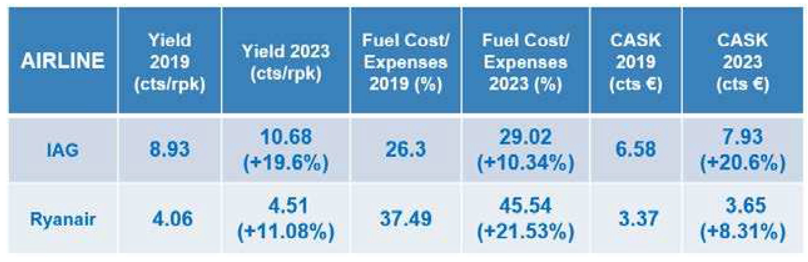
Table 5.6 shows figures of 2023 (partial) vs 2019 of IAG (September 2023) and Ryanair (June 2023). Almost all figures have improved. Despite fare increases, the demand has increased, especially the leisure segment. IAG yield has increased 19.6% and Ryanair 11.1%. In the case of Ryanair, booked passengers have increased 13% in 2023 vs 2019, and IAG is expected to increase around 2% passengers in 2023 vs 2019, with strong demand for leisure travel [23,24]. In that case, demand elasticity forecast does not hold.
In both airlines, the margin to increase CASK is slightly above the 2019 one (+15.7% vs 14.7% IAG, and +17.4% vs 14.5% Ryanair). Yield and CASK of IAG in 2023 have both about the same increase (around +20% vs 2019). Ryanair yield increase in 2023 is 2.8pp over the CASK one, which indicates improved efficiency. The fuel cost related to OEs of Ryanair jumps to 45.54% (+22%) and IAG increased to 29.02% (+10%). This means that the impact of any fuel price increase due to SAF is worse for Ryanair and may be worse for tourism.
As a further research, figures with the fuel increase impact due to SAF at the end of 2023 can be updated, since this is a dynamic system. In any case, rules should be the same for all airlines to avoid unfair competition.
6. Conclusions
6.1. Final Synthesis
In uncertain and turbulent times, with rapid and continuous changes, it is necessary to distinguish what goes unchanged (the basics, the business concept) from what must change.
In summary, the problems because some airlines have disappeared or have been absorbed can be summarized in the following two points:
- They were not aware of the break–even curve, which is the indicator of the necessary changes. They lacked the business concept and the ability to react, not knowing what to do or how to do it.
- Had they known what to do, they lacked the leadership and management capabilities to know how to do it. They did not have the leadership capability to design, persuade and convince anyone about the change or putting it into practice.
Consequently, the solution is to have a deep understanding of the airline business concept. Relocating the break–even curve, with all its implications in the management model (cost restructuring, cultural change, etc.), and knowing how to join the world of concepts with the world of things in its twofold way: knowing what needs to be done (business knowledge) and knowing how to implement it (leadership factor).
In addition, the brake–even curve also provides a clear indicator of the cost impact due to new boundary conditions, i.e., the new Environment Regulations on fuel cost due to SAF. The brake–even curve is a sound basis to demonstrate what cost impact of new regulations are unaffordable to maintain service continuity.
In summary, the brake–even curve provides two ways of usefulness: indication to move the break–even curve down to face and overcome the more efficient competitors, and to show the red lines not to surpass to address new boundary conditions like new environment regulations.
For further research, it could be interesting to evaluate the break–even curve for short and medium haul versus the long haul one. This study includes figures for both, where the different scale range in terms of yield and unit cost can be seen. In the case of network airlines, it would be useful research to evaluate the reciprocal contribution of short and medium haul and long-haul operation to the global results of the airline, and how those results can vary according to different contributions of both networks. It would be of particular interest to do research concerning the impact of a potential limitation of short and medium haul operations to reduce carbon emissions (already implemented in France) to feed the long-haul network, and its effect on global results. Also, it would be of interest to study different scenarios of fuel cost increase impact on fares, considering the demand elasticity that might apply. The net carbon zero target can be a passionate challenge for air transport to preserve the planet, to connect the world with clean energy.
6.2. Application to Other Industries
The business concept and joining concepts with things has been described and applied for the airline industry. Nevertheless, it is also applicable and can be extrapolated to other industries and organizations, both private and state-owned.
As particular cases, the equation (1) of results can be applied directly to other transport modes; and it is also applicable to hotels industry, in whose case must be substituted by available room day and the by revenue per occupied room day.
Defining the business concept of a company may not be trivial but it is inspiring and feasible, because it represents an intellectual effort of human dimensions. It is therefore applicable to all kinds of industries and organizations. When defining the business concept, it is of paramount importance to count on the participation of the management team and people from other levels, multidisciplinary. Defining the business concept includes identifying what goes unchanged and what needs to change; and if possible, identifying the value of what stays, the basics, which also illustrates what needs to change.
Joining the world of concepts with the world of things allows to see many more things in those same things. Formulating the business concept is luminous and its application is powerful; it provides certainty and trust, the virtues of know-how.
Conflicts of Interest
The authors declare no conflict of interest.
References
- IATA. Economics’ chart. 2022, December.
- https://www.iata.org/en/iata-repository/publications/economic-reports/2023-to-bring-further-pax-recovery-but-softer-cargo/ (accessed 12 May 2023).
- US Airline Deregulation Act. 1978.
- Meyer, J.R., et al. Arline Deregulation. The Early Experience. Auburn House Publishing Company. Boston, Massachusetts. 1981, pp. 71-72, 89-90, 115-118.
- Meyer, J.R., Oster, C.V. et al. Deregulation and the Future of Intercity Passenger Travel. The MIT Press. Cambridge, Massachusetts. 1987, pp. 39-41, 55-58, 80-82, 124.
- Meyer, J.R., Oster, C.V. et al. Deregulation and the New Airline Entrepreneurs. The MIT Press. Cambridge, Massachusetts. 1984, pp. 3-9.
- Gillen, D., et al. Airlines within airlines: Assessing the vulnerabilities of mixing business models. Research in Transportation Economics. 2008, 24, 25-35. [CrossRef]
- Debyser, A. Air transport: market rules. 2022. https://www.europarl.europa.eu/factsheets/en/sheet/131/air-transport-market-rules (accessed on 2 May 2022).
- EU. European Union Mobility and Transport – Air. 2023. https://transport.ec.europa.eu/transport-modes/air_en (accessed 2 May 2023).
- Porter, M.E. What is strategy? Harvard Business Review. 1996, November/December, 61-78.
- Pearson, J., et al. The strategic capability of Asian network airlines to compete with low-cost carriers. Journal of Air Transport Management. 2015, 47, 1–10. [CrossRef]
- ICAO. Annual Report of the Council. 2019. https://www.icao.int/annual-report-2019/Pages/the-world-of-air-transport-in-2019.aspx (accessed on 12 May 2023).
- Statista, 2023. https://www.statista.com/statistics/1118397/air-passenger-transport-european-union/ (accessed on 12 May 2023).
- OAG. Low-Cost Carriers in the Aviation Industry: What are they? September 2023.
- Low-Cost Carriers In The Aviation Industry: What Are They? | OAG (accessed 14 September 2023).
- Moir, L. et al. A quantitative means of comparing competitive advantage among airlines with heterogeneous business models: Analysis of U.S. airlines. Journal of Air Transport Management. 2018, 69, 72-82. [CrossRef]
- James, G.W. Airline Economics. Lexington Books, D.C. Heath and Company. Lexington, MA. 1982, pp. 57-85.
- Iberia. Annual Report. 2010. http://media.corporate-ir.net/media_files/IROL/24/240949/Informe_Anual_2010.pdf (accessed 12 May 2023).
- Iberia. IAG Annual Report. 2019. https://www.iairgroup.com/en/newsroom/press-releases/newsroom-listing/2020/financial-results-2019 (accessed 2 May 2023).
- Norwegian. Annual report. 2019. https://www.norwegian.com/globalassets/ip/documents/about-us/company/investor-relations/reports-and-presentations/annual-reports/annual-report-norwegian-2019.pdf (accessed 12 May 2023).
- Porter, M.E. Competitive Advantage. The Free Press, New York. 1985, pp. 14, 33-70, 512.
- Aviaco. Annual Report. 1992.
- Iberia. Annual Report. 1992.
- KPMG. Airline Disclosures Handbook. KPMG International. 2013, Switzerland. https://assets.kpmg.com/content/dam/kpmg/cl/pdf/2013-02-kpmg-chile-audit-ifrs-revelacion-ilustrativa-aerolinea.pdf (accessed 12 May 2023).
- Ryanair, Q1 2023 Financial Report (June 2023).
- https://investor.ryanair.com/wp-content/uploads/2023/07/Q1-FY24-Ryanair-Results.pdf (accessed 30 November 2023).
- 24. IAG. Financial Results Jan – Sep 2023.
- https://otp.tools.investis.com/clients/uk/international_airlines_group/rns/regulatory- story.aspx?cid=2457&newsid=1728494 (accessed 30 october 2023).
- 25. EasyJet. Annual Report. 2019. https://corporate.easyjet.com/~/media/Files/E/Easyjet/pdf/investors/results-centre/2019/eas040-annual-report-2019-web.pdf (accessed 2 May 2023).
- 26. Ryanair. Annual Report, March 2019. https://investor.ryanair.com/wp-content/uploads/2019/07/Ryanair-2019-Annual-Report.pdf (accessed 12 May 2023).
- 27. British Airways. IAG Annual Report. 2019. https://www.iairgroup.com/en/newsroom/press-releases/newsroom-listing/2020/financial-results-2019 (accessed 2 May 2023).
- 28. Virgin Atlantic, 2019. Annual Report. https://flywith.virginatlantic.com/content/dam/corporate/Virgin%20Atlantic%20Annual%20Report%202019_Final.pdf (accessed 12 May 2012).
- 29. Goleman, D. Leadership That Gets Results. Harvard Business Review. 2000, March/ April, 17-28.
- 30. Kotter, J.P. Leading Change. Harvard Business School Press. Boston, Massachusetts. 2012, pp.3-34.
- 31. Bridges, W. Leading Transition: A New Model for Change. 2013. http://www.crowe- associates.co.uk/wp-content/uploads/2013/08/WilliamBridgesTransitionandChangeModel.pdf (accessed 11 May 2023).
- 32. ICAO 41 Assembly Resolution A41-21. Consolidated statement of continuing ICAO policies and practices related to environmental protection – Climate Change. October 2022.
- 33. ATAG. atag-beginners-guide-to-saf-edition-2023.pdf (accessed 28 November 2023).
- 34. EU. PE-CONS 29/23 Regulation of the European Parliament and of the Council on ensuring a level playing field for sustainable air transport (ReFuelEU Aviation). 20 September 2023.
- 35. IAG investment on SAF. https://www.iairgroup.com/en/newsroom/press-releases/newsroom-listing/2023/nova-pangaea (accessed November 2023).
Figure 3.1.
Graphic representation of the results of an airline. This figure shows the results () in relation to the business variables of yield (), Load Factor () and unit cost .
Figure 3.1.
Graphic representation of the results of an airline. This figure shows the results () in relation to the business variables of yield (), Load Factor () and unit cost .
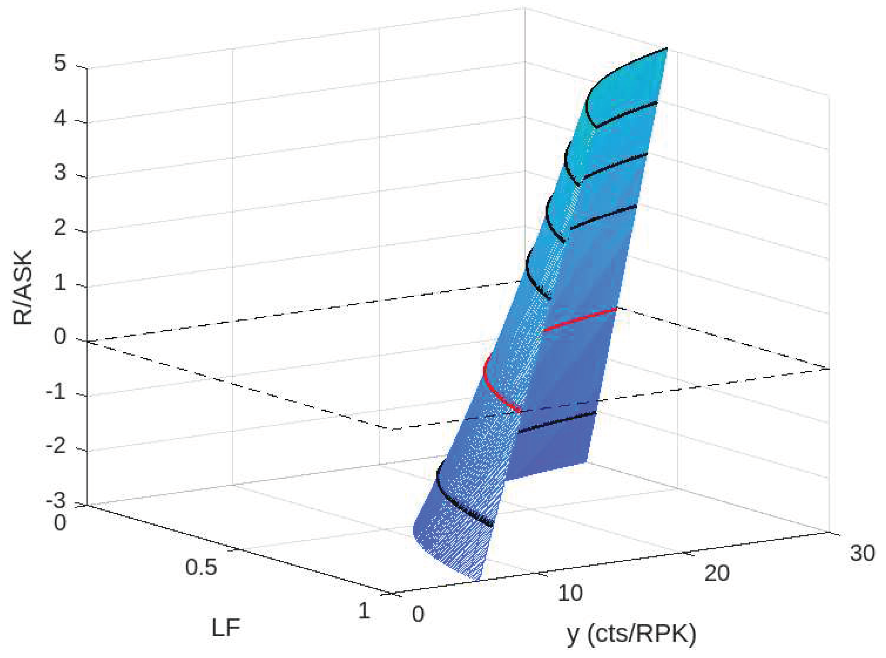
Figure 3.2.
Break–even curve for short and medium haul, with a high unit cost (), typical of a European airline before the liberalization of air transport.
Figure 3.2.
Break–even curve for short and medium haul, with a high unit cost (), typical of a European airline before the liberalization of air transport.
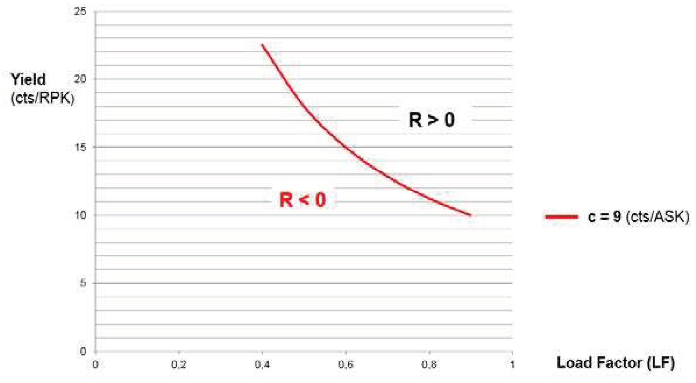
Figure 4.1.
Short and medium haul break–even curves for an established airline before full liberalization in Europe (A) and a new entrant LCC (C).
Figure 4.1.
Short and medium haul break–even curves for an established airline before full liberalization in Europe (A) and a new entrant LCC (C).
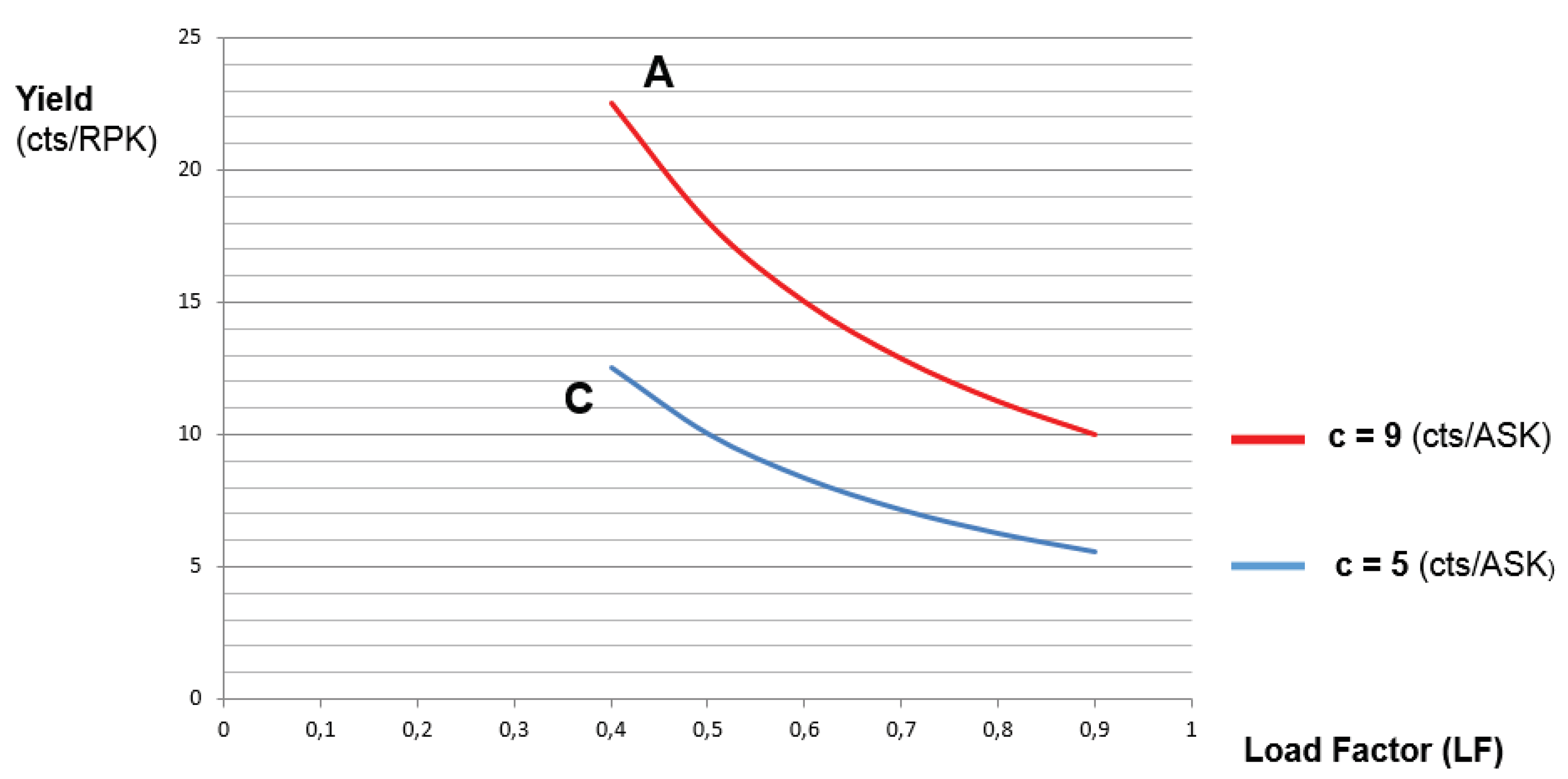
Figure 4.
2. Change of commercial zone (CZ) of airline A, changing yield and (indicated by blue arrow)
Figure 4.
2. Change of commercial zone (CZ) of airline A, changing yield and (indicated by blue arrow)
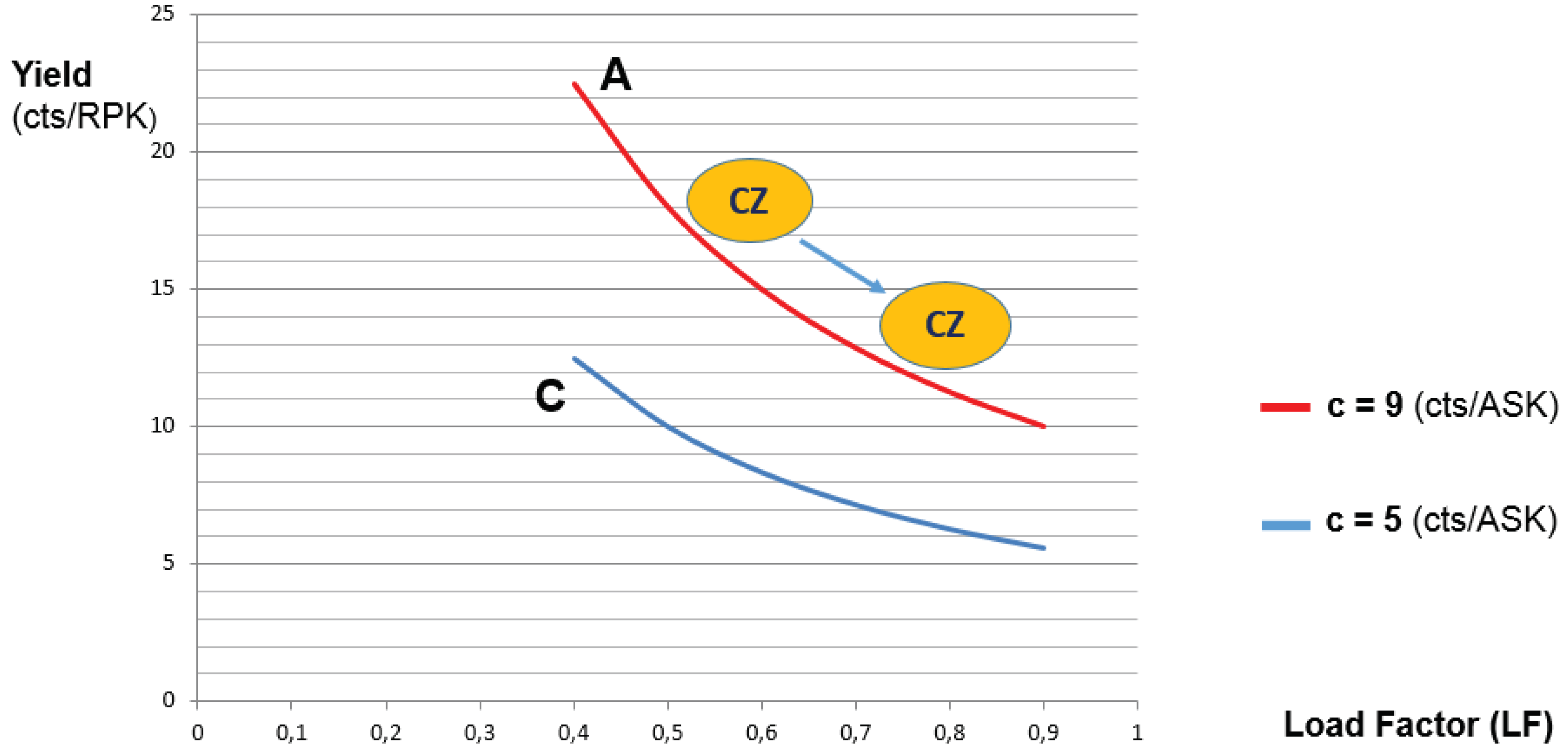
Figure 4.3.
Airline A: moving its break–even curve down to the airline C one, and CZ change.
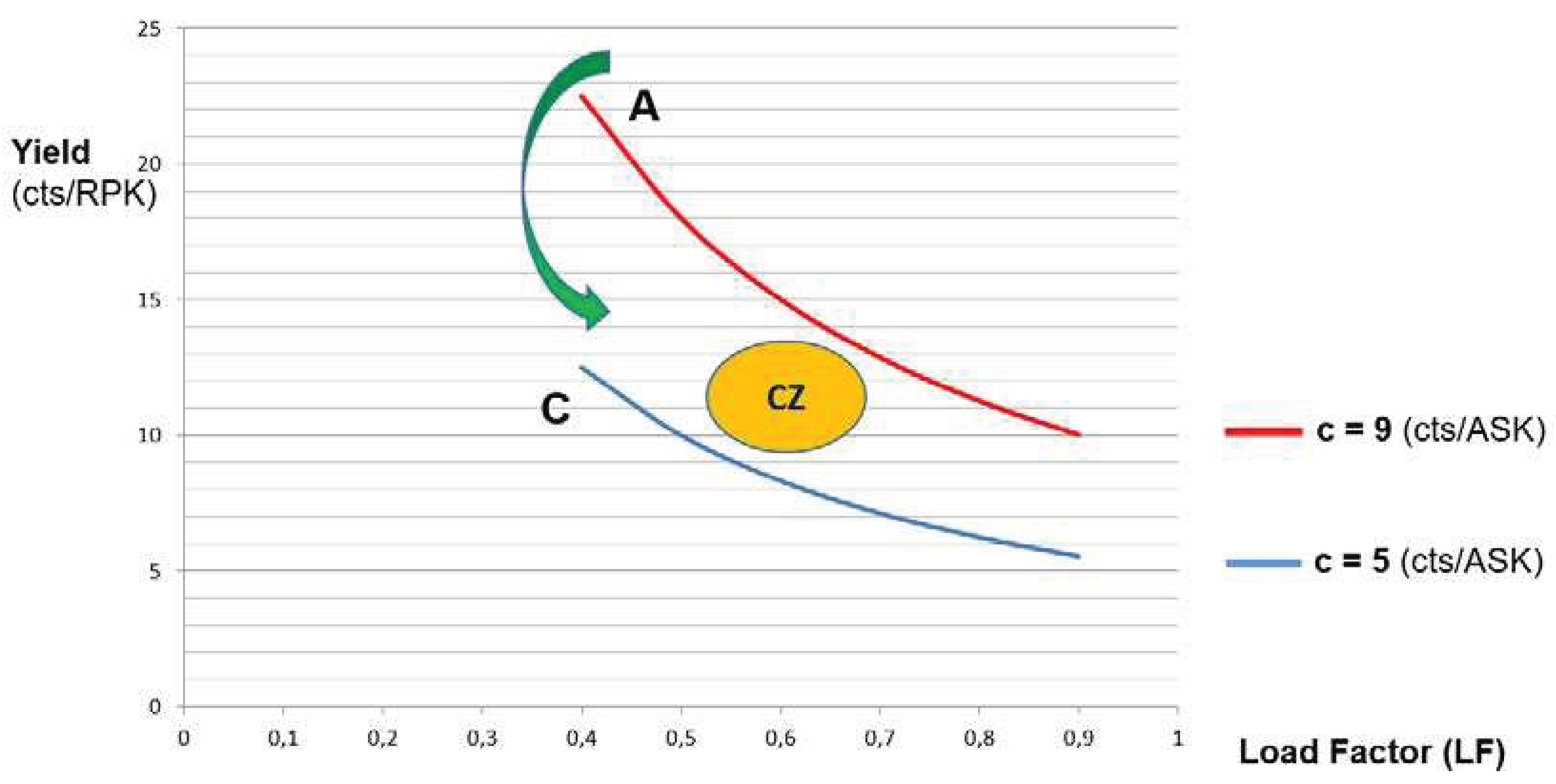
Figure 4.
4. Break-even curves for network (blue) and point-to-point (green) airlines operating a mix of short, medium and long haul.
Figure 4.
4. Break-even curves for network (blue) and point-to-point (green) airlines operating a mix of short, medium and long haul.
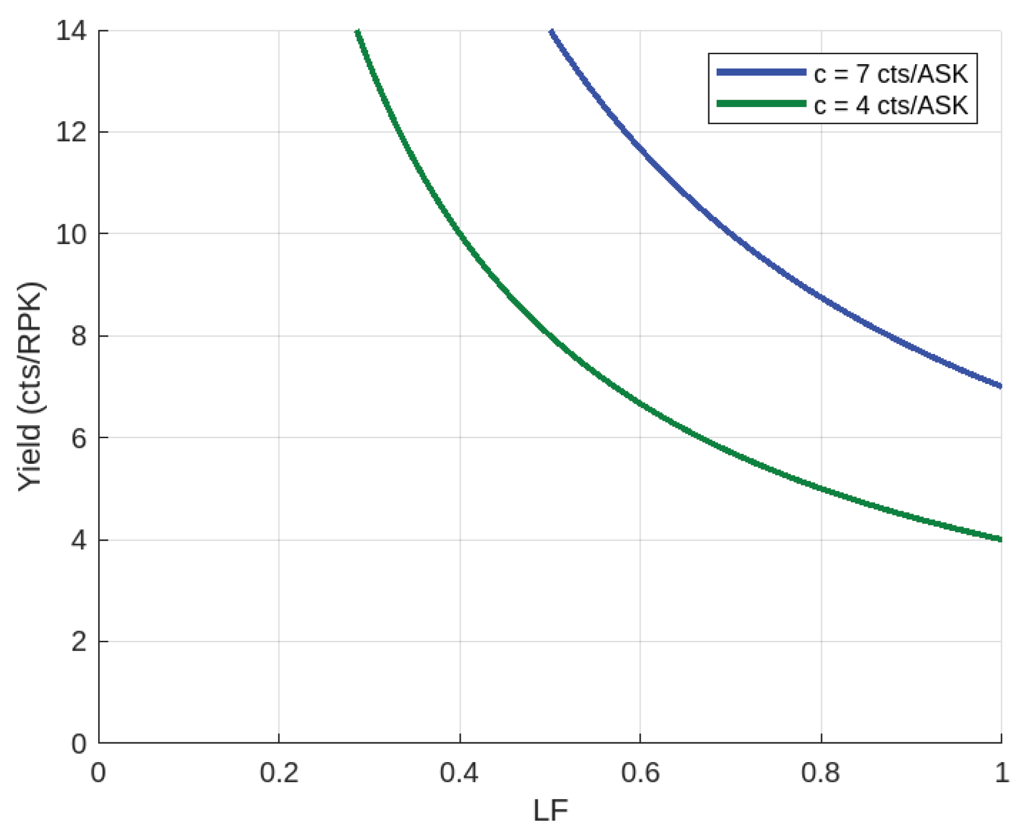
Figure 5.1.
CO2 emissions reduction plan (source: Air Transport Action Group, ATAG, April 2023 [33]).
Figure 5.1.
CO2 emissions reduction plan (source: Air Transport Action Group, ATAG, April 2023 [33]).
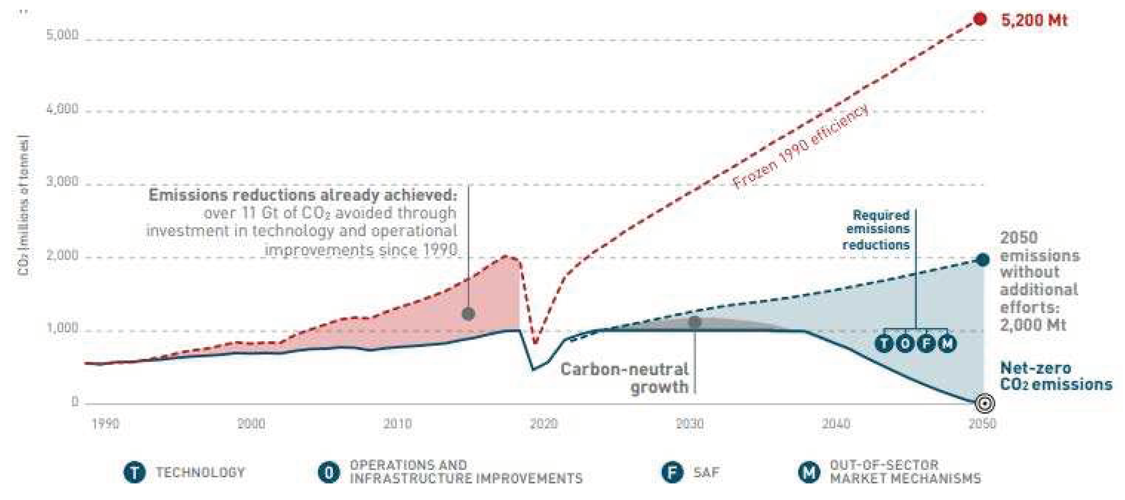
Figure 5.2.
Price evolution allowance emission per CO2 ton. (Source: Trading Economics, may 2023).
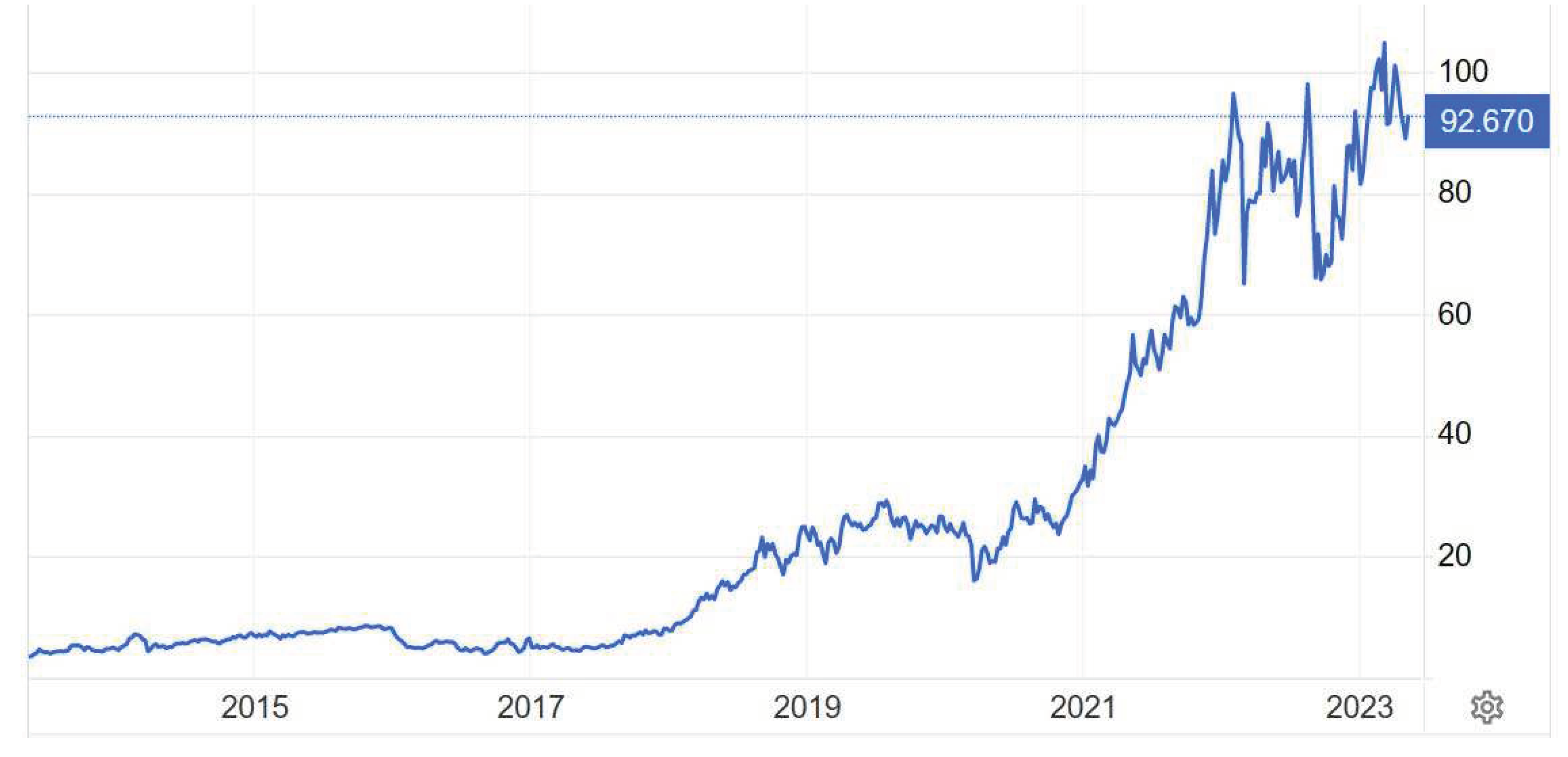
Figure 5.3.
Margin of CASK increase between the two generic curves to maintain positive results.
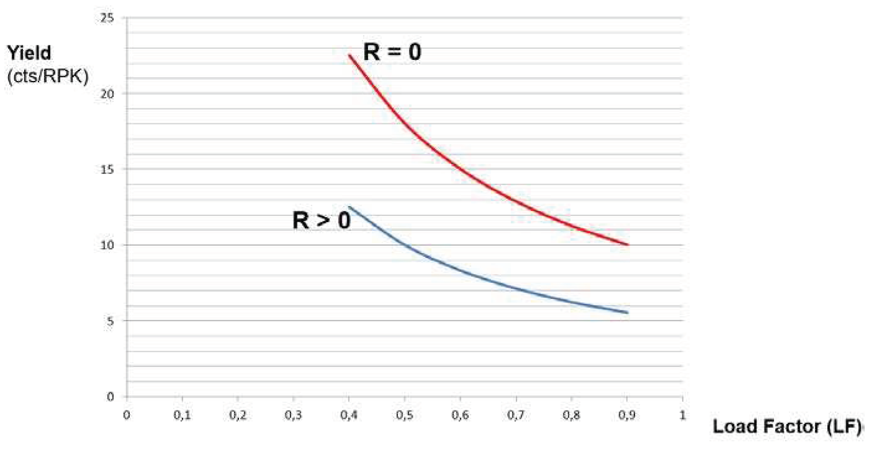
Figure 5.4.
IAG break–even curves to show CASK margin increments (2019).
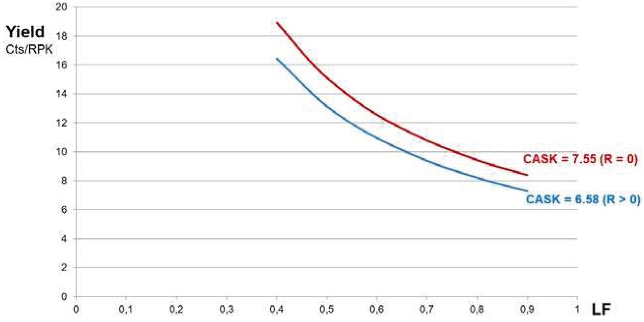
Figure 5.5.
Ryanair break–even curves to show CASK margin increments (2019).
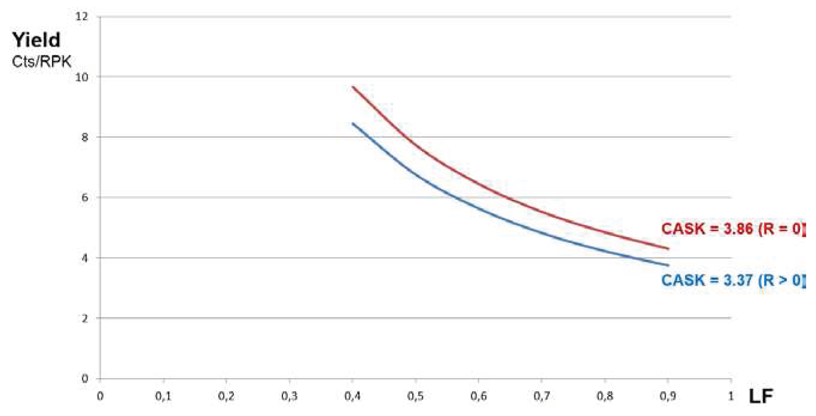
Figure 5.6.
Bar charts for IAG and Ryanair to show CASK increments according to SAF prices.
Figure 5.7.
Bar charts for IAG and Ryanair to show CASK increments according to 70 % blending SAF and different prices.
Figure 5.7.
Bar charts for IAG and Ryanair to show CASK increments according to 70 % blending SAF and different prices.
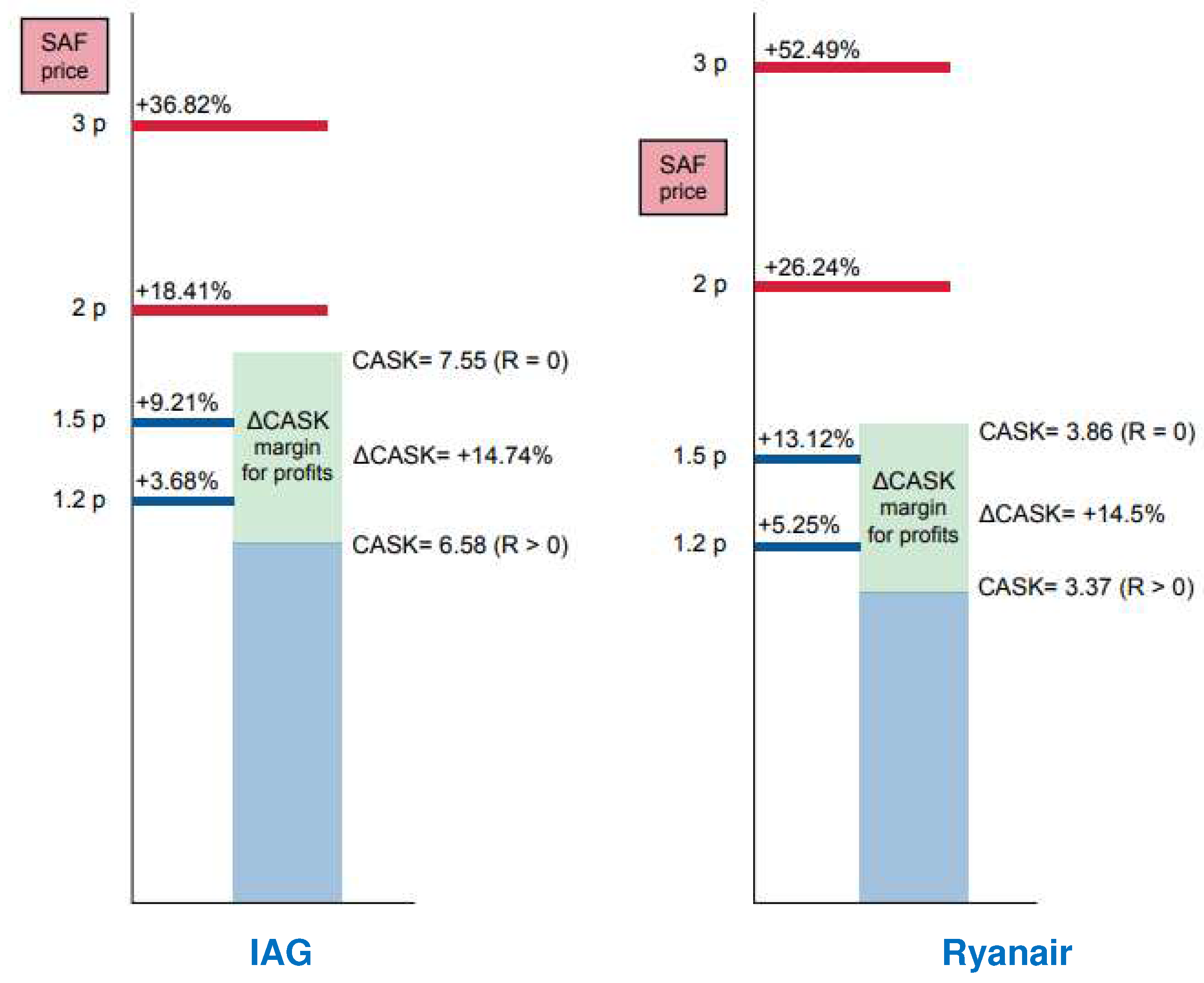

Table 1.1.
Different business data of network and point-to-point LCC airlines (2019). Source: Annual Reports of each airline (currency in Euros, €).
Table 1.1.
Different business data of network and point-to-point LCC airlines (2019). Source: Annual Reports of each airline (currency in Euros, €).
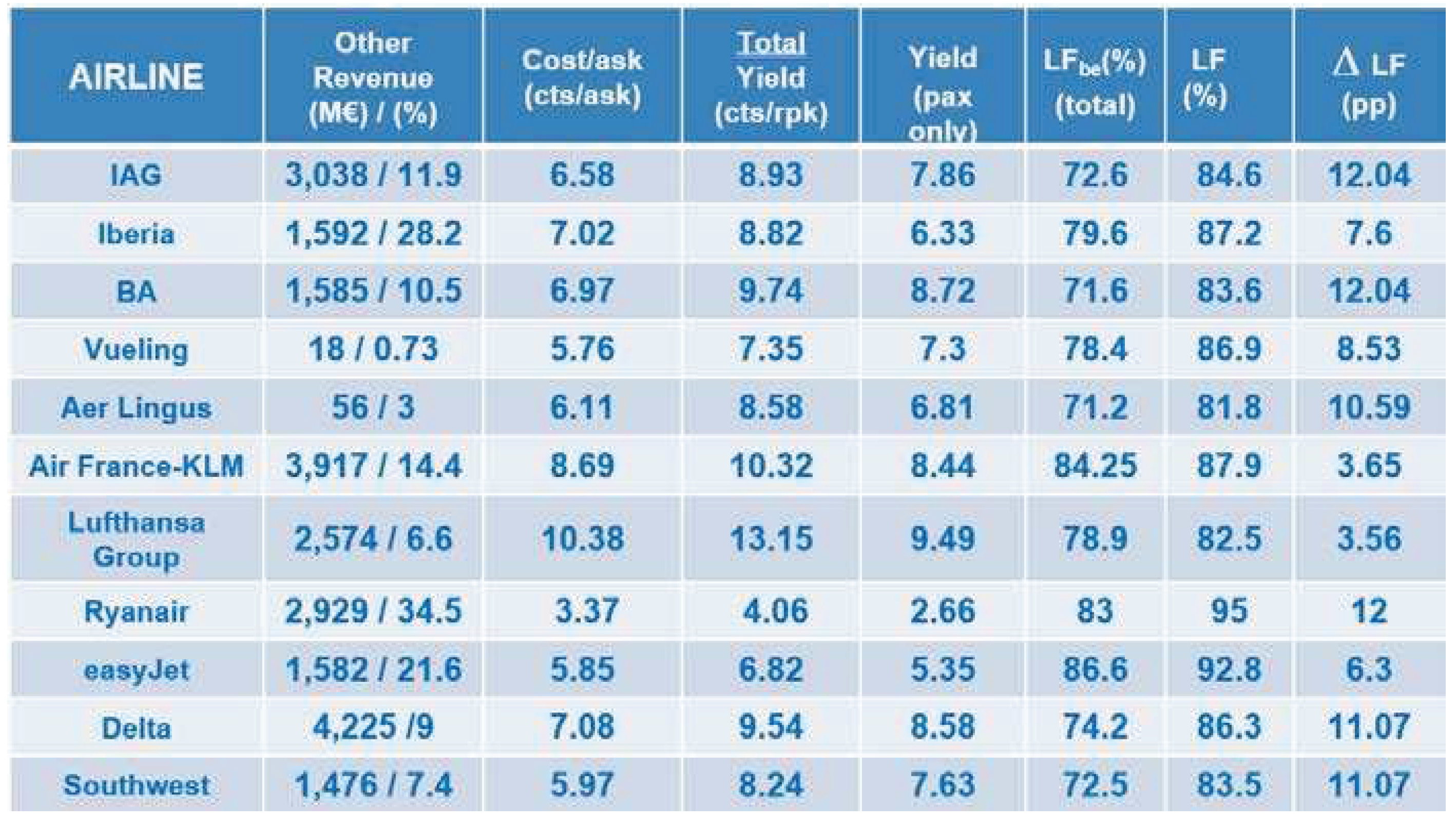
Table 1.2.
Financial performance of several airlines (both network and LCCs) in 2019, including Aena (Spanish Airport Authority).
Table 1.2.
Financial performance of several airlines (both network and LCCs) in 2019, including Aena (Spanish Airport Authority).
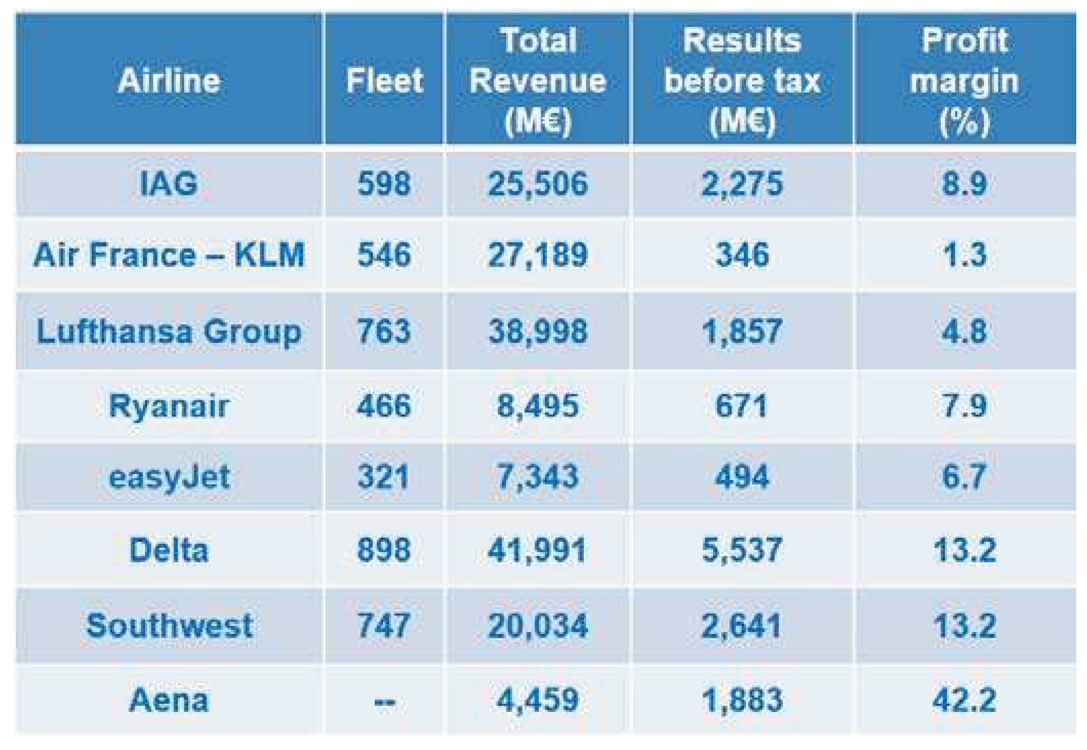
Table 5.1.
Financial indicators related to fuel cost (2019).
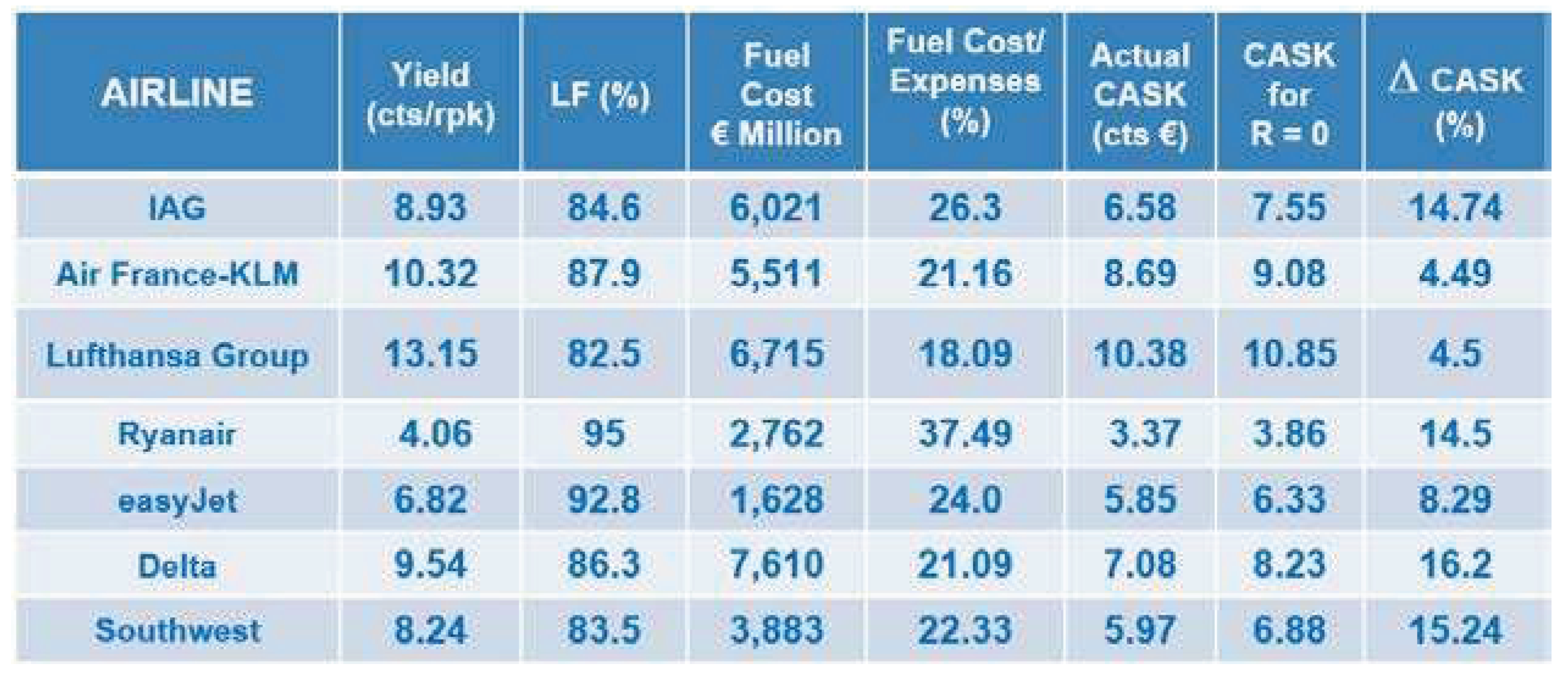
Table 5.2.
CASK increment due to SAF fuel for different prices.
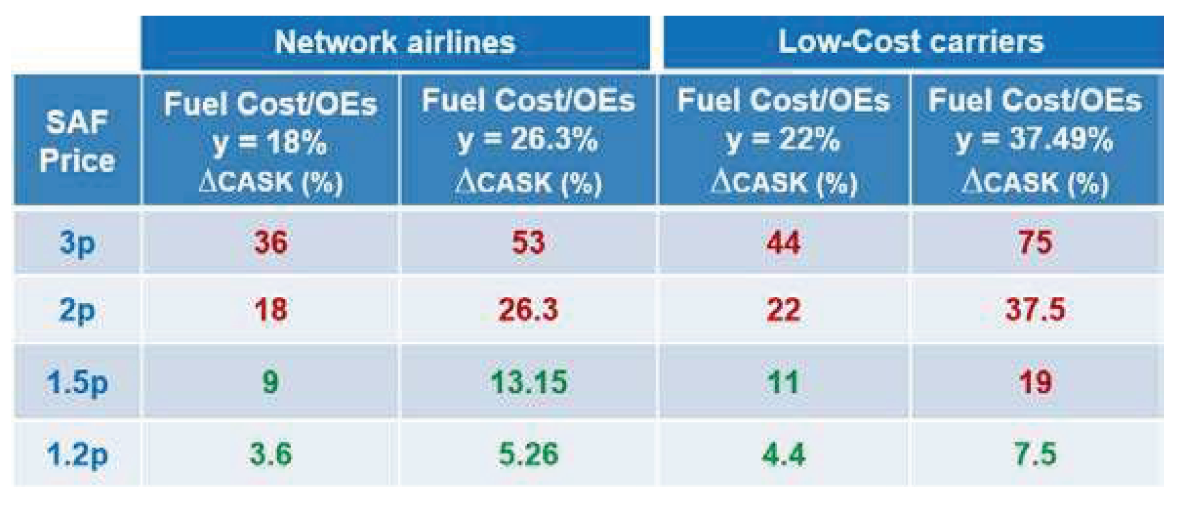
Table 5.3.
CASK increment due to SAF prices for different airlines.
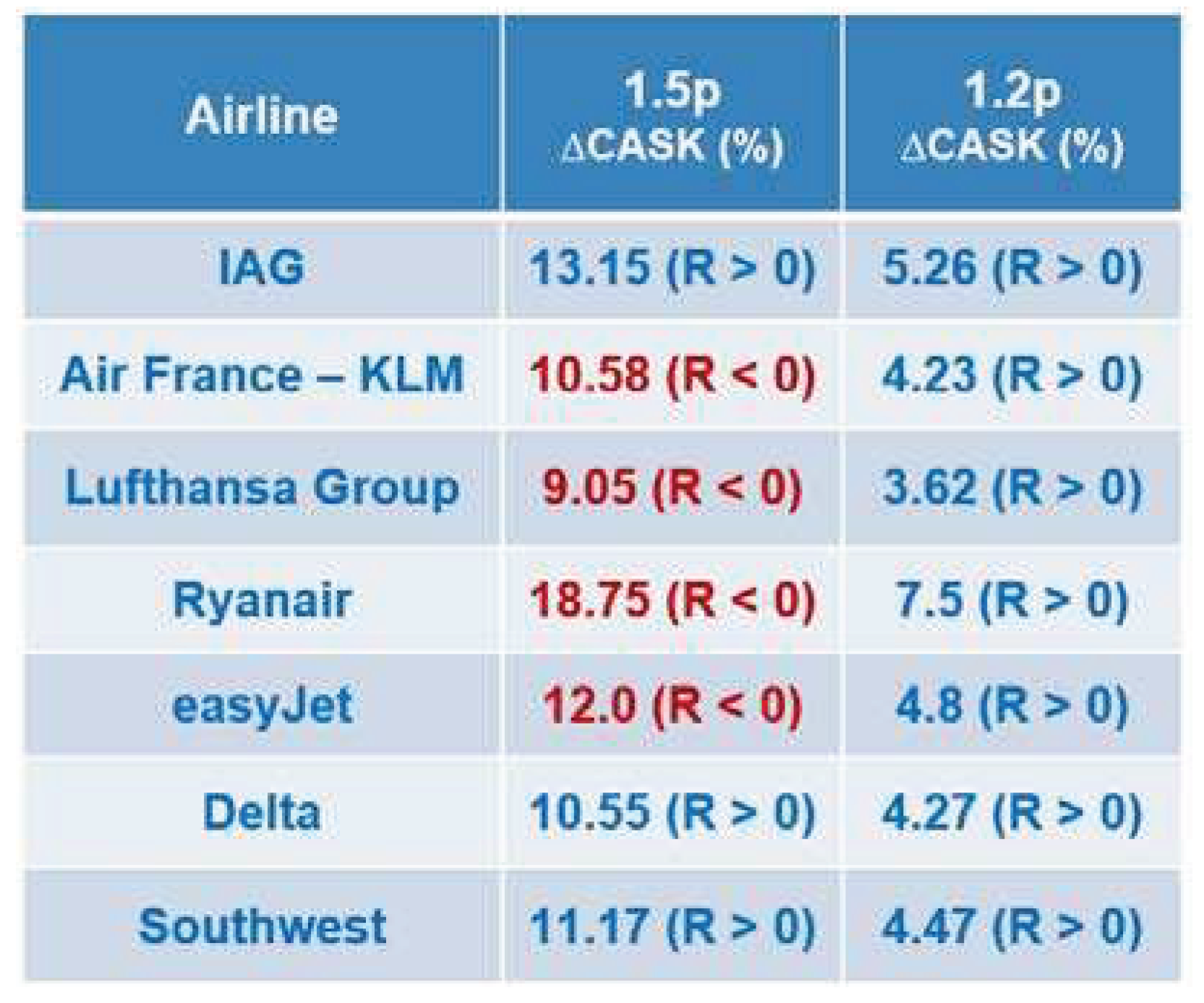
Table 5.4.
Effect on fuel cost increment for different SAF prices and blending.
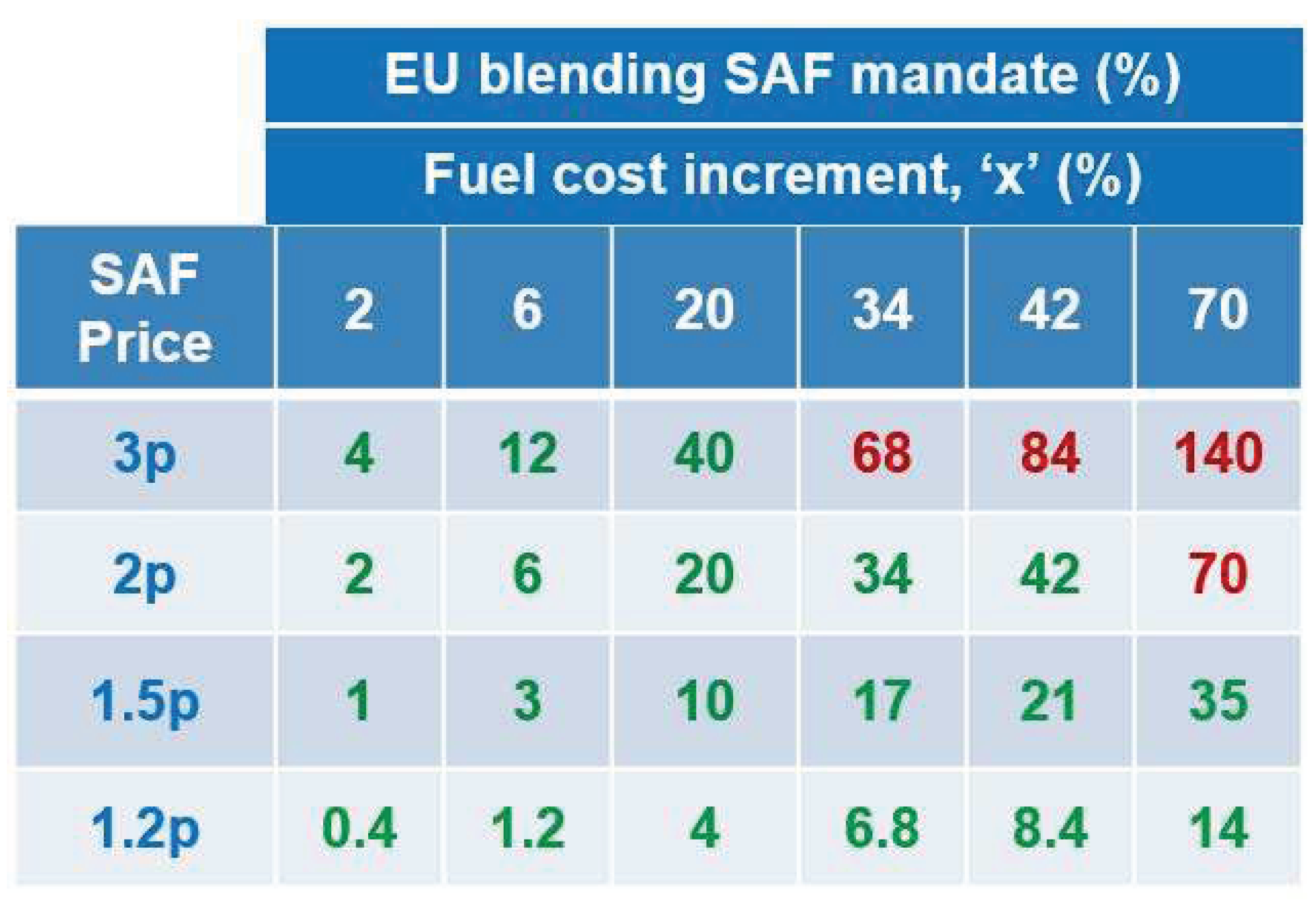
Table 5.5.
CASK increment for different airlines with 70% blending SAF.
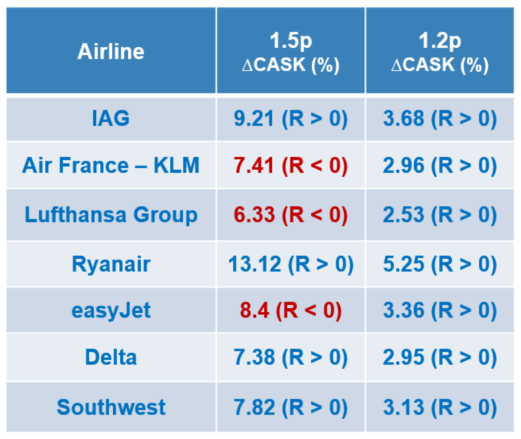
Table 5.6.
Some business data of 2023 (partial).
Disclaimer/Publisher’s Note: The statements, opinions and data contained in all publications are solely those of the individual author(s) and contributor(s) and not of MDPI and/or the editor(s). MDPI and/or the editor(s) disclaim responsibility for any injury to people or property resulting from any ideas, methods, instructions or products referred to in the content. |
© 2024 by the authors. Licensee MDPI, Basel, Switzerland. This article is an open access article distributed under the terms and conditions of the Creative Commons Attribution (CC BY) license (http://creativecommons.org/licenses/by/4.0/).
Copyright: This open access article is published under a Creative Commons CC BY 4.0 license, which permit the free download, distribution, and reuse, provided that the author and preprint are cited in any reuse.


