

Submitted:
17 January 2024
Posted:
18 January 2024
You are already at the latest version
Abstract
A primary challenge in isogeny-based cryptography lies in the substantial computational cost associated to computing and evaluating prime-degree isogenies. This computation traditionally relied on Vélu’s formulas, an approach with time complexity linear in the degree but which was further enhanced by Bernstein, De Feo, Leroux, and Smith to a square-root complexity. The improved square-root Vélu’s formulas exhibit a degree of parallelizability which has not been exploited in major implementations. In this study, we introduce a theoretical framework for parallelizing isogeny computations and provide a proof-of-concept implementation in C with OpenMP. While the parallelization effectiveness exhibits diminishing returns with the number of cores, we still obtain strong results when using a small number of cores. Concretely, our implementation shows that for large degrees it is easy to achieve speedup factors of up to 1.74, 2.54 and 3.44 for 2, 4 and 8 cores, respectively.
Keywords:
isogenies
; elliptic curves
; parallelism
; postquantum cryptography
; efficient implementation
1. Introduction
Since the foundational work of De Feo, Jao and Plût [1,2], which resulted in the SIKE protocol [3], isogeny-based cryptography has received considerable interest in the development of post-quantum cryptography. Today, the security of SIKE has been broken by a wave of attacks which started with the work of Castryck and Decru [4] and was followed up by the works of Maino, Martindale, Panny, Pope, and Wesolowski [5] and of Robert [6], ultimately demonstrating the existence of a polynomial-time attack on SIKE with any starting curve. Nevertheless, there are still many isogeny-based protocols that remain unbroken, including the CSIDH [7] key exchange protocol and signature schemes like SeaSign [8], CSI-Fish [9] and SQISign [10], the last of which is currently under consideration in the NIST (National Institute of Standards and Technology) process for Standardization of Additional Digital Signature Schemes [11].
While SIKE only required the computation of isogenies of degrees 2 and 3, there has been a tendency in some of the newer isogeny-based protocols to move towards higher and higher prime degrees. This has brought increasing attention to the task of optimizing the evaluation of large-degree isogenies. For instance, the original CSIDH proposal used isogenies of degrees up to 587, and Chávez, Chi, Jacques and Rodríguez have suggested that a level 5 dummy-free implementation would need degrees as high as 2239 [12] after revising the security. More recently, the level 5 version of SQISign that was submitted to the NIST standarization process [13] brings the ceiling up with a colossal degree-318233 isogeny computation. Even the aforementioned attacks on SIKE require the evaluation of large prime-degree isogenies, with the techniques from [5] requiring the evaluation of an isogeny of degree 321193 over a large extension field for a direct key recovery attack. Therefore, optimizing the computation of large prime-degree isogenies is of great interest for constructive purposes as well as for cryptanalysis. Interestingly, a new generation has also risen of isogeny-based protocols which utilize the techniques of the attack constructively, such as FESTA [14], QFESTA [15], IS-CUBE [16] and constructions for VDFs [17] and VRFs [18], of which the last two also involve large-degree isogenies.
Traditionally, the main method for computing isogenies of prime degree ℓ when there exists a point of order ℓ in the curve has been Vélu’s formulas, initially introduced in [19] and expanded upon in [20] and [21]. In view of the ubiquitousness of large-degree isogenies, the more recent improvement from Bernstein, De Feo, Leroux, and Smith [22], which reduced the time complexity from to , has been a keystone for the viability of many protocols. In addition to the straightforward savings that it provides, this new algorithm also exhibits a substantial degree of parallelizability that has remained largely unexplored.
- Our Contributions. In this work we detail and showcase the parallelizability of the square-root Vélu formulas, focusing on the problem of computing a single large-degree isogeny from a fixed kernel generator and pushing a number of points through said isogeny. We analyze and provide a parallelism-friendly reformulation of the square-root Vélu formulas, and provide a proof-of-concept (PoC) implementation to illustrate the implications of our work. More precisely,
- We propose a new indexing system for the points in the kernel of the isogeny that is similar to the one presented in [22], but which can be naturally split into subsets that are assigned to each core in a multi-core implementation.
- We provide a parallelized expected cost function based on our square-root Vélu variant, as well as a revised expected cost of the sequential Vélu formulas that were presented in [23]. Assuming that the assigned task is to perform an isogeny construction and to push two points through it, the idealized speedup factors for large degrees is up to 1.79, 2.96 and 4.58 faster than the expected sequential cost function using two, four and eight cores, respectively.
- We give a PoC implementation utilising C and OpenMP to compute our isogeny formulas with large odd prime degrees. Our implementation assumes for concreteness that isogenies are evaluated over a prime field such that there exist rational points of the desired degree in the curve, and achieves speedup factors for large degrees of up to , and for 2, 4 and 8 cores, respectively, even for medium-sized isogenies.
- Assumptions and generalizations. For the purposes of our implementation, we have searched for a 1792-bit prime such that contains evenly-spaced prime factors ranging from 19 to 321193 (the degree of the isogeny in the attack of [5]). Isogenies are performed over the base prime field, and two points are pushed through each isogeny. These choices were made for concreteness and closely mirror the scenario in CSIDH. On the other hand, they do not adhere exactly to the case of SQISign (which works in a quadratic field extension) nor that of the attack in [5] (which performs isogenies in a much larger field extension). Nevertheless, the techniques that we describe save on a fixed number of field multiplications, which are the dominating part of the total cost. Therefore we expect that similar speedups in percentage would be obtained in those other cases, with the caveat that the savings could even be slightly larger as the parallelization overhead becomes more negligible with respect to the arithmetic cost. As for the theoretical savings, our costs are expressed in terms of the total number of field multiplications and remain valid for any choice of base field.
- Related Work. Different forms of parallelism have been explored at various layers of isogeny-based protocols. For instance, the use of vectorization through Intel’s Advanced Vector Extensions (AVX-512) has been exploited for the finite field arithmetic layer, both in the context of CSIDH [24] and of the now obsolete SIKE protocol [25,26], obtaining speedup factors in the order of . Additionally, it has also been proposed to use AVX-512 to batch multiple evaluations of the protocols, leading to increases in throughput of up to for CSIDH [24] and in SIKE [26]. When latency is the focus, vectorization can also be used to push multiple points through an isogeny, leading to the concept of parallel-friendly evaluation strategies which favour pushing points over point multiplications [26,27,28]. These parallel strategies can accelerate the evaluation of large composite-degree isogenies, but do not apply for isogenies of a large prime degree.
This work focuses exclusively on the multi-core optimization for the isolated evaluation of a large prime-degree isogeny, which has received much less attention. To the best of our knowledge, there are only simple parallelization strategies that have been proposed [29] for the linear-complexity Vélu formulas, not exploiting the improved complexity methods from [22]. We also do not consider vectorization: if it was to be used, we expect that the best way to exploit it would be at the field arithmetic layer. This would lead to improvements similar to those from [24,25,26] which are well documented and are largely parallel to our multi-core improvements.
- Outline. The remainder of the manuscript is organized as follows. In Section 2 we give the basic background and description of the original square-root Vélu formulas with their three main building blocks: KPS, xISOG and xEVAL, and derive their expected cost function. In Section 3 we introduce our new framework, explaining the need for a new indexing system in Section 3.1 and then detailing the new algorithms in Section 3.2 and deriving their expected cost function in Section 3.3. Finally, in Section 4, we present our experimental results, comparing the performance to the theoretical savings.
2. Background
We denote by the finite field with elements, and p a prime number. We focus on supersingular Montgomery curves, E, given by
Remark 1.
In general, a Montgomery curve is defined by the equation such that and , but all choices of B are equivalent up to isomorphism. For the sake of simplicity, we write instead of and omit the constant B.
Viewing the curve as a projective surface, the set of -rational points in E forms a group where the point at infinity ∞ acts as the group identity. An order-d point P on E is a point on the curve such that d is the smallest positive integer satisfying
We write to refer to the d-torsion subgroup of E.
- Isogenies. An isogeny is a surjective morphism between curves with a finite kernel such that . Such a map is always also a group homomorphism. Two curves E and are isogenous over if there exists such connecting them, or equivalently if . The kernel of is , denoted by . When restricting only to separable maps, the degree of an isogeny is equal to the size of its kernel, and an isogeny is uniquely determined by its kernel up to an isomorphism. An isogeny of degree ℓ is referred to as a ℓ-isogeny, and it has a unique dual (up to isomorphism) of the same degree such that and are equivalent to the multiplication-by-ℓ map on E and , respectively.
2.1. Computation of ℓ-Isogenies
Let be a Montgomery curve defined over and a point of order ℓ. If is an isogeny with ker, then it is possible to find polynomials such that
The polynomials and are related by a formula stated by Elkies [30], so the main task for computing an ℓ-isogeny is that of obtaining from P. In the particular case of Montgomery curves, from the formulas of [31] the coefficient of the Montgomery curve can be obtained by,
and the x-coordinate of the point , by
where and .
In 2020, Bernstein, De Feo, Leroux and Smith [22] proposed an important improvement in the computation of isogenies. Their key idea exploits the fact that for isogeny evaluations and constructions, it is not required to compute the polynomial h itself, but only its evaluation at a given set of points. We briefly describe their method for evaluating (1) and (2), starting by pointing out that, although the map is not holomorphic, an algebraic relation exists between the values. More precisely,
Lemma 1
([22] Lemma 4.3). Let be an elliptic curve, where q is a prime power. There exist biquadratic polynomials , , and in such that
for all P and Q in E such that .
This allows us to rearrange in a baby-step giant-step style:
where the index system is chosen such that , with and satisfying the following definition:
Definition 1.
Let S, I and J be finite sets of integers. The is an index system of S if:
- 1.
- the maps defined by and are both injective and have disjoint images.
- 2.
- and are both contained in S.
From here, they show that the factor of that is related to I and J can be computed efficiently as a resultant. More precisely, letting be the union of the sets and , the following result is proven.
Lemma 2
([22] Lemma 4.9). Let be an elliptic curve, where q is a prime power. Let P be an order-n element of . Let be an index system such that and do not contain any elements of . Then
where
and where .
Remark 2.
Notice that is precisely the first parenthesis that appears in (3), which can be computed quadratically faster as a resultant, while the second parenthesis (corresponding to ) is a leftover product that is still computed in linear time. Based on this, Adj, Chi-Domínguez, and Rodríguez-Henríquez [23] introduced three explicit algorithms for evaluating ℓ-isogenies: KPS (which computes the necessary multiples of the kernel generator), xISOG (which obtains the coefficient of the image curve) and xEVAL (which obtains the image of a point). These algorithms are reproduced here as Algorithm 1, Algorithm 2 and Algorithm 3.
| Algorithm 1 KPS |
|
| Algorithm 2 xISOG |
|
| Algorithm 3 xEVAL |
|
2.2. Computing the Resultants
The main computational task that is required for the square-root Vélu algorithm is the evaluation of the resultants , which can be achieved in constant-time via a remainder tree approach as described in [23]. This task accounts for approximately 85% of the total computation time, and depends on the size of the sets I, J, and K. For the following discussion, we set , and . As a remainder, if splits into linear factors as and , then the resultant is given by
For our purposes, the polynomials f and g are provided as a product of linear polynomials and b quadratic polynomials, respectively. Since the values are readily available, one could compute (4) directly by evaluating g multiple times, but this would lead to a complexity of .
Instead, we begin by obtaining the polynomials f and g as a list of coefficients by multiplying together all the terms following a product tree approach, as shown in Figure 1.
After the product tree for f has been built, we compute a corresponding reciprocal tree. Unlike the product tree, the reciprocal tree is computed from the root down. If a node in the product tree contains a polynomial F of degree m, then the corresponding node in the reciprocal tree contains , where is a polynomial of degree m and c is a constant such that . Here, denotes the polynomial with the list of coefficients in reverse order: if , then . The reciprocal tree is depicted in Figure 2, and is used as an auxiliary tool to construct one last tree called the residue tree.
The residue tree is also built from the root down, and as depicted in Figure 3, each of its nodes contains , where F is the polynomial in the corresponding node of the product tree of f and c the constant from the reciprocal tree. The leaves of the remainder tree contain a multiple of , so a multiple of the resultant is readily obtained by multiplying all the leaves together. The multiple cancels out when taking the ratios at the last step of Algorithm 3 and Algorithm 2. Remarkably, this method allows us to compute (a multiple of) all of the with a complexity of just . A detailed description for the cost of the product tree, reciprocal tree, and remainder tree is presented in the Appendix A.
2.3. Cost model for the Sequential Square-Root Vélu
An expected cost function for KPS, xISOG, and xEVAL has been presented in [23], but it takes into account some redundant computations and also fails to consider the cost of the remainder tree. We now present a more accurate and optimal cost function.
As in [23], we begin by noting that a better performance is achieved when is as small as possible and are similar in size. Since we need to have , we set the size of to be and then perform division with remainder to obtain and . For simplicity, from now on we ignore rounding errors and assume the average value for , so that .
Next, we provide explicit formulas for the number of field multiplications in each of the three procedures as a function of b. This cost model neglects the cost of field additions and subtractions, as well as the savings that a field squaring may have over a regular field multiplication. We consider this a fair compromise, since the total number of squarings is small and the benefit of having a single metric far outweighs the importance of the small error. The cost functions are expressed in terms of the cost of the various tree procedures, which are detailed in the Appendix A.
- Cost function for KPS. Notice that the computation of is performed in both Algorithm 3 and Algorithm 2, so instead we delegate this product tree and the corresponding reciprocal tree to KPS and perform it only once. The total cost of KPS is then reflected by obtaining b multiples of an elliptic curve point (at a cost of field multiplications each) for each of , and , and the cost of a product tree and reciprocal tree for b linear polynomials. We obtain
- Cost function for xISOG. The degree-2 factors in and can be obtained at the cost of field multiplications, and the complete polynomials are then obtained from two product trees of quadratic leaves. We then perform 2 residue trees to compute the two resultants of Algorithm 2, and another multiplications to compute and . Algorithm 2 also requires an ℓ-th power exponentiation at an average cost of multiplications, which must be performed separately on the numerator and denominator when working in projective coordinates. Finally, there are another 10 multiplications for the final two steps. We obtain
- Cost function for xEVAL. In this case, computing the factors for requires field multiplications. However, only one product tree is required since can be obtained by inverting the coefficient list of , as noted in [23]. We then need two residue trees to compute the resultants in Algorithm 3, multiplications to compute and , and 6 more multiplications for the final step. The total is
- Total cost function. The total cost function, assuming that two points need to be pushed through the isogeny as is the case in CSIDH and SQISign, is
3. Parallelizing Square-Root Vélu Formulas
In this section, we present our main results which focuses on the problem of parallelizing Vélu’s formulas for isogeny computations.
An immediate observation is that the two resultants that appear in each of Algorithm 2 and Algorithm 3, which represent the heaviest part of the computation, are completely independent of each other. Therefore, there is a simple way to parallelize the two algorithms in a 2-core implementation by assigning one resultant to each core. We show that these algorithms exhibit a good degree of parallelizability even beyond two cores, by assigning more than one core per resultant. However, doing so requires a new indexing system that allows for a clear separation of the computation between cores, which we introduce in the first subsection.
Additionally, other parts of the algorithms are also apt for parallelization, such as the computation of and where a partial product can be assigned to each core, or the computation of product trees where a subtree can be assigned to each core after a small bit of sequential work. We show also that the computation of point multiples in KPS can be parallelized with our new index system.
After detailing the new index system, provide explicit new algorithms for the square-root Vélu formulas which can be computed by assuming the availability of n-cores, where is a power of two.
3.1. Construction of a New Index System
The main observation that allows us to parallelize the computation of resultants beyond two cores is that they exhibit a multiplicative property. More precisely, if I can be written as the disjoint union
then
so we can assign one subset to each of the cores, have them compute one subresultant each, and then multiply them all together. Doing so will require us to modify the sizes of I and J: since each resultant computation should have balanced sizes, we now require . Accordingly, we now need and . We will design such an indexing system according to the following lemma.
Lemma 3.
Let be a power of two, ℓ be an odd positive integer and consider the set . If and , then is an index system for S, where
Moreover, if and only if
Proof of Lemma .
Suppose that
where , and and (t and can be equal). Then,
so
but this is impossible since and thus . Therefore, the map defined by is injective. Similarly, the map is injective and therefore, both have disjoint images.
On the other hand, the sets and are both contained in S. It is clear that the elements in these sets are odd integers. Since for all , and we have the following:
Similarly, for all , and since the minimum of I is when and the maximum of J is when . □
Note that we have chosen to partition I into only subsets because, when n cores are available, we assign cores to each of the two resultants. However, when computing point multiples during KPS we do have all n cores available for working on the subsets. Therefore, it will be convenient to further divide each into two subsets to obtain a total of n half-sized subsets. Note that some subsets will have fewer elements than others because need not be a multiple of n. In practice, this is problematic because it is crucial for each core to perform exactly analogous tasks to guarantee performance. In order to achieve a balanced computation, we will add additional elements to the subsets that are lacking, ensuring that each subset contains the same number of elements, while ignoring redundant multiples in future steps. This idea is inspired by [22] and the parallelization technique proposed by Costello in [32] to compute the set . We provide an example to illustrate this approach.
Example 1.
So and . Instead of this, we can consider the following sets:
So , , and .
Let and . From the Lemma 3 we get
We will now demonstrate that the partitioning of the set I, without taking into account the additional elements added to ensure equal-sized subsets, still forms an index system.
Proposition 1.
then In particular, () is an index system for S.
Let us assume the same conditions of the Lemma 3. Let . If
Proof of Proposition 1.
If is an even integer, it is clear that , for all and thus . Note that and considering that and I have the same cardinality, we conclude that they are equal. If is an odd integer, all we have that . When , dropping the last element in each , we have . Note that the cardinality of is and the cardinality of is . □
Similarly, we consider a partition of into n sets with elements,
However, when is not divisible by n, we will add one additional element to each set , ensuring that each subset contains the same number of elements.
The additional elements that were added to balance the size of the sets are not taken into account when calculating the corresponding products for each set.
3.2. Parallelized Algorithms
We now describe the construction of parallelized versions of algorithms KPS, xISOG, and xEVAL assuming that n cores are available, which we refer to as KPS-Parallel, xISOG-Parallel, and xEVAL-Parallel.
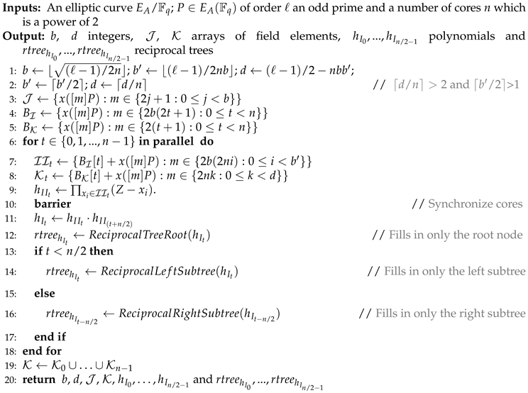
The KPS-Parallel algorithm, presented as Algorithm 4, is based on the new index system from Proposition 1: instead of computing the sets and as in the original algorithm, KPS-Parallel computes the sets and , as well as the polynomial product tree for , by assigning one core to each value of . Note that the computation of the resultants requires a reciprocal tree for each of the , so the polynomials are multiplied pair-wise to obtain the polynomials . We then compute the residue trees, which are built from the root down: the root is computed for each tree using cores, and then the two subtrees of each tree are computed in parallel, using two cores per tree, for a total of n cores. Note that although the computations for the root of the product and reciprocal trees, corresponding to lines 11 and 12 of 4, should only be ran with cores, we instead have all cores running with half of them repeating the work over dummy arrays for . These computations are of course redundant, but ensure that the workload is balanced.
| Algorithm 4 KPS-Parallel |
 |
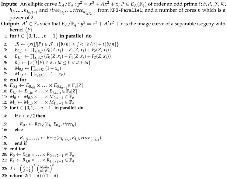
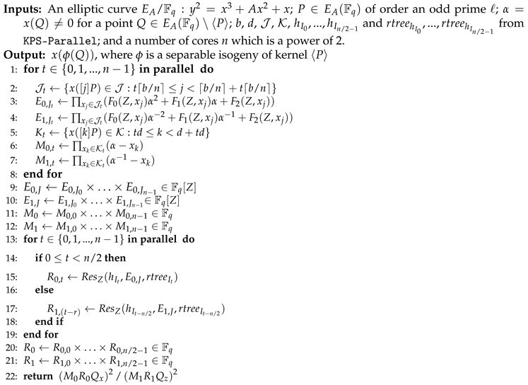
For the algorithms xISOG-Parallel and xEVAL-Parallel, the set J is partitioned into n subsets , and each core computes the polynomial product tree corresponding to one subset. The roots of the n trees are then multiplied together sequentially to obtain the full polynomial . Next, each core computes one of the subresultants using the reciprocal trees from KPS-Parallel, and the subresultants are multiplied sequentially at the end to obtain the two principal resultants. As for the computations related to , it is also split into subsets so that each core can compute a subproduct of , and the subproducts are multiplied together at the end.
| Algorithm 5 xISOG-Parallel |
 |
In the next subsection, we present a detailed analysis that estimates the cost of computing the image curve of an isogeny and the evaluation of a point using the procedures KPS-Parallel+ xISOG-Parallel+ xEVAL-Parallel.
| Algorithm 6 xEVAL-Parallel |
 |
3.3. Cost Analysis of the Parallel Square-Root Vélu
In this section, we will provide an estimation of the cost that is expected when performing the KPS-Parallel, xISOG-Parallel, and xEVAL-Parallel procedures, which is analogous to the one presented in subSection 2.3 for the sequential algorithms. Recall that for our new index system from subSection 3.1 we have , where ℓ is the degree of the isogeny and n represents the number of cores available, while each of the subsets has a size of for a total size of . It follows that
As before, we will ignore rounding errors and assume that takes the middle value of this range (neglecting the second term), so that , , and for .
Proposition 2.
The cost of computing the parallel AlgorithmKPS-Parallelwith n cores is
field multiplications.
Proof of Proposition 2.
In order to find all the point multiples in K, we first compute the first n multiples sequentially and then core t start from the t-th multiple and take steps of size n. This leads to wall-clock time of point operations, which involve 6 field multiplications each. A similar approach is taken for computing all the multiples in the sets, while the ones in are computed sequentially as this is the smallest of the sets. A product tree is constructed for each of the in parallel, and line 11 involves multiplying two polynomials of degree b/2. As for the reciprocal trees, we incur the cost of the root node and then just half of the remainder cost since there is one core working on each subtree, so its cost is (Reciprocal(b) + ReciprocalTree(b))/2, where Reciprocal(b) = blog2(3) + b + 2log2(b) − 2 is the cost of the root node alone. The total cost is then
and the proposition follows after considering the cost functions in the Appendix A.
□
We now focus on Algorithm 5:xISOG-Parallel which computes the coefficient of the image curve, and on Algorithm 6:xEVAL-Parallel which computes the isogeny evaluation at a specific point.
Proposition 3.
The cost of computing the parallel AlgorithmxISOG-Parallelwith n cores is
field multiplications.
Proof of Proposition 3.
We begin by considering the cost of computing the polynomials and in Algorithm 5, where comes from KPS-Parallel. We partition into the subsets of size each, and compute one sub-product tree per subset concurrently. The cost of computing the factors of each subset is given by field multiplications, then a product tree is computed for quadratic polynomials on each core, and the tree roots are multiplied together sequentially to obtain the complete polynomial . This last step involves multiplying together n polynomials of degree each, which we denote as . An identical procedure is used to compute as well.
Using the residue trees from KPS-Parallel, each core then compute a subresultant using a residue tree of size , and the subresultants are multiplied sequentially at a cost of multiplications per resultant.
For each of the , each core computes a subproduct of size b at a cost of multiplications, and then combining the subproducts takes another multiplications.
Finally, we use two cores to compute the ℓ-th power exponentiation in Algorithm for the numerator and denominator concurrently at a cost of about , and the last few products take 10 more multiplications.
The total cost is then
and the proposition follows after considering the cost functions in the Appendix A. □
Proposition 4.
The cost of computing the parallel AlgorithmxEVAL-Parallelwith n cores is
field multiplications.
Proof.
The proof of the current proposition follows a similar structure to the previous proposition, with the main distinction lying in the polynomials and . As before, the factors of can be computed with a cost of , and only one product tree is needed since is obtained at no additional cost. For each of and , each core is still working with a subset of size b, but now there is a cost of b scalar multiplications for computing the factors in a subset, for the subproduct of each subset, and for combining the subproducts. There is no exponentiation in this case, and the final steps require only 6 additional multiplications. The total cost is then
and the proposition follows after considering the cost functions in the Appendix. □
The next theorem summarizes our cost analyzis, and follows immediately from the previous propositions.
Theorem 1.
The expected total cost of the algorithmsKPS-Parallel,xISOG-Paralleland twicexEVAL-Parallelexpressed in field multiplications, assuming that two points need to be pushed through the isogeny, is given by
4. Experimental Results
We implemented our parallel version of the square-root Vélu algorithm in the C programming language, leveraging OpenMP for parallelization. This implementation has been integrated into a fork of the SQALE’d CSIDH library [12], where we can measure the savings due to parallelism for isogenies of each prime degree . In order to visualize the progression of the performance with the isogeny degree, we have incorporated a new 1792-bit prime
where for odd primes that are roughly evenly spaced between and (the degree of the isogeny in the attack of [5]). This prime was chosen so that isogenies of each degree can be evaluated using only arithmetic (for which we also provide an assembly code implementation). As previously mentioned, this model most closely resembles the scenario in CSIDH as opposed to applications where isogenies are performed over quadratic fields or larger extensions. However, we make this choice for concreteness while still expecting our results to extrapolate well to other scenarios since the main savings come from reducing the number of field multiplications by a factor that is agnostic to the field itself. Our library can be found at https://github.com/TheParallelSquarerootVeluTeam/Parallel-Squareroot-Velu. The benchmark results presented in this section are from experiments conducted using an Intel(R) Xeon(R) Gold 6230R processor equipped with 26 physical cores, operating at . Turbo boost and Hyper-threading technologies were disabled during these experiments.
Our experimental results are illustrated in Figure 4. We measured the total computational time for executing KPS-Parallel, xISOG-Parallel, and two iterations of xEVAL-Parallel for each of the prime degrees using 2, 4 and 8 cores, and compared to the computational time of the original sequential implementation of [12]. In Figure 4 we compare the observed speedup factors against the theoretical speedup using (6) and (5). We observe there is a more important difference for the eight-core implementation. Moreover, we notice that in situations where the degree of the isogeny is not sufficiently large, the overhead associated with synchronization and the computational steps involved tends to offset any potential performance gains achieved by employing eight cores. However, the speedup factor can be seen to achieve levels close to the asymptotic value starting from .
To showcase our results in a more practical setting, we also implemented and benchmarked our parallelized square-root Vélu algorithms in the context of SQALE’d CSIDH-9216. In its dummy-free variant, SQALE’d CSIDH-9216 performs the operations corresponding to KPS + xISOG + 2xEVAL exactly once for each of the 333 smallest odd primes (excluding 263), over a 9216-bit prime field. The experimental timings for each of the three routines, summed over all the degrees, are shown in Table 1. Our two-core implementation achieves speedup factors of 1.23, 1.70, and 1.92 for KPS-Parallel, xISOG-Parallel, and xEVAL-Parallel, respectively, while for the four-core implementation we obtained acceleration factors of 1.42, 2.27, and 3.02. While these accelerations span the entirety of the Vélu-related computations in the protocol, it is important to stress that they cannot be translated easily into an acceleration for the protocol as a whole, since the protocol includes other non-negligible computations (most notably elliptic curve point scalar multiplications).
5. Discussion
Since KPS-Parallel performs some of its computational tasks sequentially, while others only benefit from half of the total number of cores, it is not surprising that its speedup factor is the lowest out of the three square-root Vélu routines. Nonetheless, as illustrated by Table 1, this is not too important as its total cost is comparatively small. Fortunately, the largest accelerations come from the xEVAL-Parallel, which apart from being the most expensive of the three is often required to be evaluated multiple times for different points.
Both our experimental and theoretical results show that parallelizing with at least two cores yields strong improvements, which are important considering that they can be combined with other improvements such as vectorized field arithmetic. On the downside, it is also noticeable that the speedup factors in our implementations do not scale well when transitioning to four- and eight-core implementations. From eight cores onward, even the maximum speedup derived from the theoretic estimates suggests that the utilization that can be achieved may not be attractive for practical applications. The intuition behind these diminishing returns on the parallelization effectiveness is easy to explain, as the size of the resultants in algorithm 5 and 6 only decreases as .
Acknowledgments
This work started when Chávez-Saab, J. and Ortega, O. were doing an internship at the Technology Innovation Institute (TII) under the guidance of Prof. Dr. Rodríguez-Henríquez F. We thank TII for sponsoring such an internship. We thank ANID for the study scholarship to Ortega, O. grant number 21190301. We also thank Dr. Chi-Domínguez J. and Dr. Zamarripa-Rivera L. for valuable discussion on an early version of this manuscript. Additionally, this work has received partial funding to facilitate the use of a server in CINVESTAV-IPN in Mexico which was used for our tests.
Appendix A. Cost Functions for Polynomial Operations
In this section, we detail the costs in field multiplications associated with various operations in both the sequential and parallel versions of square-root Vélu.
- Polynomial Multiplication. The basic step is the multiplication of two polynomials of equal degree d, which we denote as . We use a Karatsuba strategy for polynomial multiplication, so the cost in field multiplications can be expressed as in [33]
- Multiplication of Multiple Polynomials. Suppose we want to multiply together m polynomials of degree d each. If m is small, we opt for multiplying the polynomials one by one: in step 1 we are multiplying together 2 polynomials of degree d, and in step t for we are multiplying a polynomial of degree by another of degree d. By partitioning the larger polynomial, we can perform this multiplication via t polynomial multiplications of degree d by d, so the total cost is
On the other hand, if m is large then we opt for a product tree strategy, where the input polynomials are placed at the leaves of the tree and each node contains the product of its two child nodes. We assume for simplicity that m is a power of 2. At level i (where i=0 corresponds to the root), we need to compute nodes, each of which is a product of two polynomials of degree . The total cost is therefore
We only use product trees for computing and which have leaves of degree and , respectively, so we are only interested in the special cases
- Reciprocal tree. Computing the resultants requires the aid of a reciprocal tree, which is built from the root down using the product tree. If a node in the product tree contains a polynomial F of degree m, then the corresponding node in the reciprocal tree contains , where is a polynomial of degree m and c is a constant such that . Here, denotes the polynomial with the list of coefficients in reverse order: if , then .
We only use the case for the product tree of a polynomial f that has b leaves of degree 1. For the root of the tree, we need to know the cost of obtaining from scratch , where f has degree b. As pointed out in [23], if we have already computed a reciprocal of half the degree (that is, ), then the inverse modulus can be obtained as with
These equations can be evaluated at the cost of field multiplications (for multiplying by the scalar ), plus the cost of 2 polynomial multiplications modulus (because the term in parenthesis is known to have null coefficients for all powers less than ), plus one squaring. This leads to the recursive formula for the cost of the reciprocal
The base case (finding a multiple of the reciprocal of a constant) is trivial, so we obtain
The child nodes in the reciprocal tree can then be computed from the root. Let be polynomials of degree d corresponding to sibling nodes of the product tree, and assume that we have already computed a reciprocal for their parent node . That is, we already have such that . It follows that , so we can compute a reciprocal for via the modular multiplication . The total cost of the reciprocal tree is then
- Residue tree. Recall that we can compute the resultant for monic f aswhere are the roots of f and are its linear factors. In the context of 2 and 3, (resp. the parallel versions 5 and 6), f is a polynomial of degree b corresponding to (resp. ) for which we have already computed the product tree with leaves as well as the reciprocal tree, and g is a polynomial of degree corresponding to for which we have computed the product tree with leaves of degree 2. We obtain the values by building a residue tree from the root down. Each node of the residue tree contains , where F and G are the polynomials in the corresponding nodes of the product trees of f and g, respectively, and c is the constant of the reciprocal tree.
As pointed out in [34], the computation of for can be achieved with the aid of from the reciprocal tree via
at the cost of an additional two polynomial multiplications modulus , so the total cost of the tree (including the cost to multiply together all of the leaves) is
Note that the product of all the leaves gives us a multiple of the resultant (the multiple being the product of all the c constants at the leaves of the reciprocal tree), but these cancel out when taking ratios in the actual algorithms.
References
- De Feo, L.; Jao, D. Towards quantum-resistant cryptosystems from supersingular elliptic curve isogenies. Post-Quantum Cryptography; Yang, B.Y., Ed.; Springer Berlin Heidelberg: Berlin, Heidelberg, 2011; pp. 19–34. [Google Scholar]
- De Feo, L.; Jao, D.; Plût, J. Towards quantum-resistant cryptosystems from supersingular elliptic curve isogenies. J. Mathematical Cryptology 2014, 8, 209–247. [Google Scholar] [CrossRef]
- SIKE - Supersingular Isogeny Key Encapsulation. Available online: https://sike.org/, 2023. Accessed: 6-12-2023.
- Castryck, W.; Decru, T. An Efficient key recovery attack on SIDH. Advances in Cryptology – EUROCRYPT 2023; Hazay, C., Stam, M., Eds.; Springer Nature Switzerland: Cham, 2023; pp. 423–447. [Google Scholar]
- Maino, L.; Martindale, C.; Panny, L.; Pope, G.; Wesolowski, B. A direct key recovery attack on SIDH. Advances in Cryptology – EUROCRYPT 2023; Hazay, C., Stam, M., Eds.; Springer Nature Switzerland: Cham, 2023; pp. 448–471. [Google Scholar]
- Robert, D. Breaking SIDH in polynomial time. Advances in Cryptology – EUROCRYPT 2023; Hazay, C., Stam, M., Eds.; Springer Nature Switzerland: Cham, 2023; pp. 472–503. [Google Scholar]
- Castryck, W.; Lange, T.; Martindale, C.; Panny, L.; Renes, J. CSIDH: An efficient post-quantum commutative group action. Advances in Cryptology – ASIACRYPT 2018: 24th International Conference on the Theory and Application of Cryptology and Information Security, Brisbane, QLD, Australia, December 2–6, 2018, Proceedings, Part III; Springer-Verlag: Berlin, Heidelberg, 2018; pp. 395–427. [Google Scholar]
- De Feo, L.; Galbraith, S.D. SeaSign: compact isogeny signatures from class group actions. Advances in Cryptology – EUROCRYPT 2019; Ishai, Y., Rijmen, V., Eds.; Springer International Publishing: Cham, 2019; pp. 759–789. [Google Scholar]
- Beullens, W.; Kleinjung, T.; Vercauteren, F. CSI-FiSh: Efficient isogeny based signatures through class group computations. Advances in Cryptology – ASIACRYPT 2019; Galbraith, S.D., Moriai, S., Eds.; Springer International Publishing: Cham, 2019; pp. 227–247. [Google Scholar]
- De Feo, L.; Kohel, D.; Leroux, A.; Petit, C.; Wesolowski, B. SQISign: Compact post-quantum signatures from quaternions and isogenies. Advances in Cryptology – ASIACRYPT 2020; Moriai, S., Wang, H., Eds.; Springer International Publishing: Cham, 2020; pp. 64–93. [Google Scholar]
- National Institute of Standards and Technology NIST. Available online: https://csrc.nist.gov/news/2023/additional-pqc-digital-signature-candidates, 2023. Accessed: 6-12-2023.
- Chávez-Saab, J.; Chi-Domínguez, J.; Jaques, S.; Rodríguez-Henríquez, F. The SQALE of CSIDH: sublinear Vélu quantum-resistant isogeny action with low exponents. J. Cryptogr. Eng. 2022, 12, 349–368. [Google Scholar] [CrossRef]
- SQIsign: Algorithm specifications and supporting documentation. Available online: https://csrc.nist.gov/csrc/media/Projects/pqc-dig-sig/documents/round-1/spec-files/sqisign-spec-web.pdf, 2023. Accessed: 6-12-2023.
- Basso, A.; Maino, L.; Pope, G. FESTA: Fast encryption from supersingular torsion attacks. Cryptology ePrint Archive, Paper 2023/660, 2023.
- Nakagawa, K.; Onuki, H. QFESTA: Efficient algorithms and parameters for FESTA using quaternion algebras. Cryptology ePrint Archive, Report 2023/1468, 2023.
- Moriya, T. IS-CUBE: An isogeny-based compact KEM using a boxed SIDH diagram. Cryptology ePrint Archive, Report 2023/1506, 2023.
- Decru, T.; Maino, L.; Sanso, A. Towards a Quantum-resistant Weak Verifiable Delay Function. Progress in Cryptology - LATINCRYPT 2023 - 8th International Conference on Cryptology and Information Security in Latin America; Aly, A.; Tibouchi, M., Eds. Springer, 2023, Vol. 14168, LNCS, pp. 149–168.
- Leroux, A. Verifiable random function from the Deuring correspondence and higher dimensional isogenies. Cryptology ePrint Archive, Report 2023/1251, 2023.
- Vélu, J. Isogénies entre courbes elliptiques. Comptes-Rendus de l’Académie des Sciences, Série I 1971, 273, 238–241. [Google Scholar]
- Kohel, D.R. Endomorphism rings of elliptic curves over finite fields. PhD thesis, University of California at Berkeley, The address of the publisher, 1996. Available at:http://iml.univ-mrs.fr/~kohel/pub/thesis.pdf.
- Washington, L. Elliptic curves: number theory and cryptography, Second Edition, 2 ed.; Chapman & Hall/CRC, 2008.
- Bernstein, D.J.; Feo, L.D.; Leroux, A.; Smith, B. Faster computation of isogenies of large prime degree. In: ANTS XIV. The Open Book Series, vol. 4(1), pp. 39–55 (2020), 2020.
- Adj, G.; Chi-Domínguez, J.; Rodríguez-Henríquez, F. Karatsuba-based square-root Vélu’s formulas applied to two isogeny-based protocols. Journal of Cryptographic Engineering 2022. [Google Scholar] [CrossRef]
- Cheng, H.; Fotiadis, G.; Großschädl, J.; Ryan, P.Y.A.; Rønne, P.B. Batching CSIDH group actions using AVX-512. IACR Transactions on Cryptographic Hardware and Embedded Systems 2021, 2021, 618–649. [Google Scholar] [CrossRef]
- Orisaka, G.; López-Hernández, J.C.; Aranha, D.F. Finite field arithmetic using AVX-512 for isogeny-based cryptography. 18th Brazilian Symposium on Information and Computer Systems Security (SBSeg), 2018, pp. 49–56.
- Cheng, H.; Fotiadis, G.; Großschädl, J.; Ryan, P.Y.A. Highly Vectorized SIKE for AVX-512. IACR Transactions on Cryptographic Hardware and Embedded Systems 2022, 2022, 41–68. [Google Scholar] [CrossRef]
- Phalakarn, K.; Suppakitpaisarn, V.; Rodríguez-Henríquez, F.; Hasan, M.A. Vectorized and parallel computation of large smooth-Degree isogenies using precedence-constrained scheduling. Cryptology ePrint Archive, Paper 2023/885, 2023.
- Phalakarn, K.; Suppakitpaisarn, V.; Hasan, M.A. Speeding-up parallel computation of large smooth-degree isogeny using precedence-constrained scheduling. Information Security and Privacy; Nguyen, K., Yang, G., Guo, F., Susilo, W., Eds.; Springer International Publishing: Cham, 2022; pp. 309–331. [Google Scholar]
- Kato, G.; Suzuki, K. Speeding up CSIDH using parallel computation of isogeny. 2020 7th International Conference on Advance Informatics: Concepts, Theory and Applications (ICAICTA), 2020, pp. 1–6.
- Elkies, N.D.; others. Elliptic and modular curves over finite fields and related computational issues. AMS IP STUDIES IN ADVANCED MATHEMATICS 1998, 7, 21–76. [Google Scholar]
- Costello, C.; Hisil, H. A Simple and Compact Algorithm for SIDH with Arbitrary Degree Isogenies. Advances in Cryptology - ASIACRYPT 2017 - 23rd International Conference on the Theory and Applications of Cryptology and Information Security, Hong Kong, China, December 3-7, 2017, Proceedings, Part II; Takagi, T.; Peyrin, T., Eds. Springer, 2017, Vol. 10625, Lecture Notes in Computer Science, pp. 303–329.
- Costello, C. B-SIDH: Supersingular Isogeny Diffie-Hellman Using Twisted Torsion. Advances in Cryptology - ASIACRYPT 2020 - 26th International Conference on the Theory and Application of Cryptology and Information Security, Daejeon, South Korea, December 7-11, 2020, Proceedings, Part II; Moriai, S.; Wang, H., Eds. Springer, 2020, Vol. 12492, Lecture Notes in Computer Science, pp. 440–463.
- Karatsuba, A.; Ofman, Y. Multiplication of Multidigit Numbers on Automata. Soviet Physics Doklady 1962, 7, 595. [Google Scholar]
- Bernstein, D.J., Fast multiplication and its applications. In Algorithmic Number Theory; Buhler, J.; Stevenhagen, P., Eds.; Mathematical Sciences Research Institute Publications, Cambridge University Press: United Kingdom, 2008; pp. 325–384.
Figure 1.
Diagram of the product tree for computing .
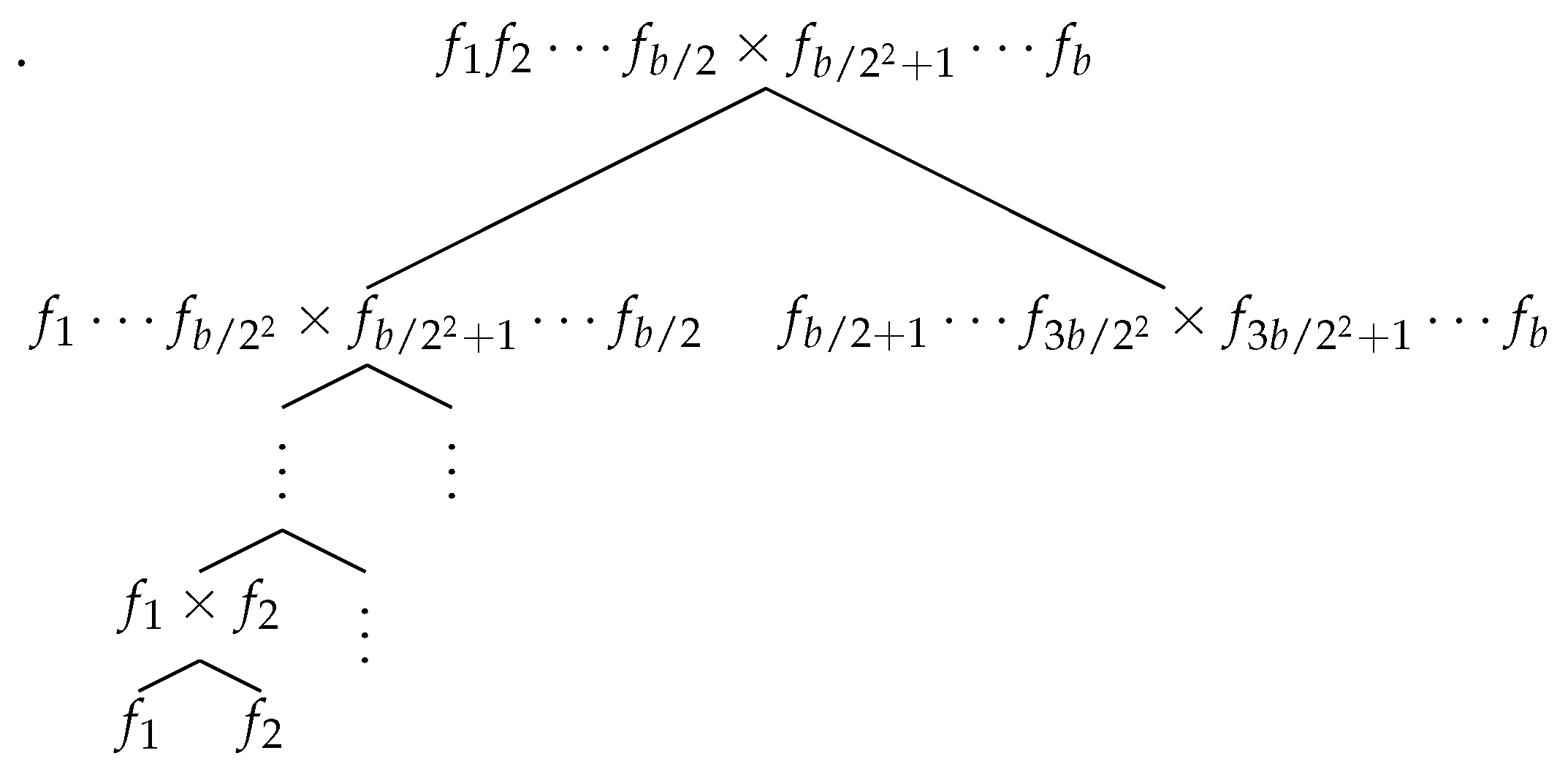
Figure 2.
Diagram of the reciprocal tree, where , and are as mentioned above.
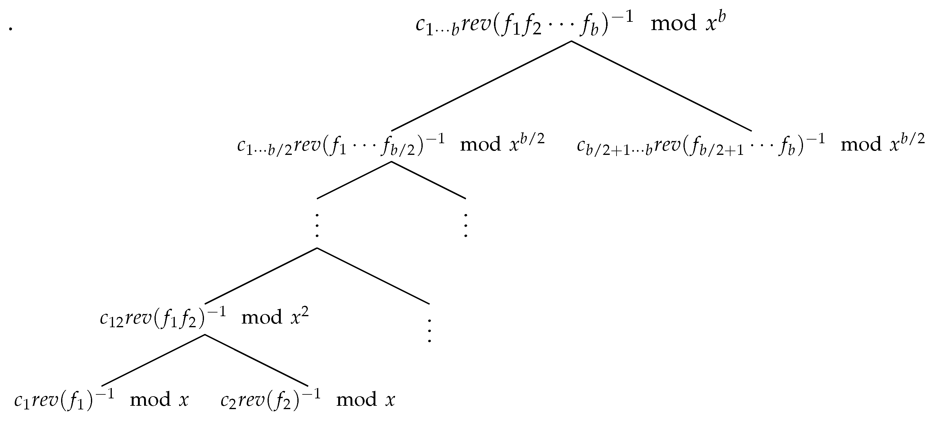
Figure 3.
Diagram of the remainder tree for computing .
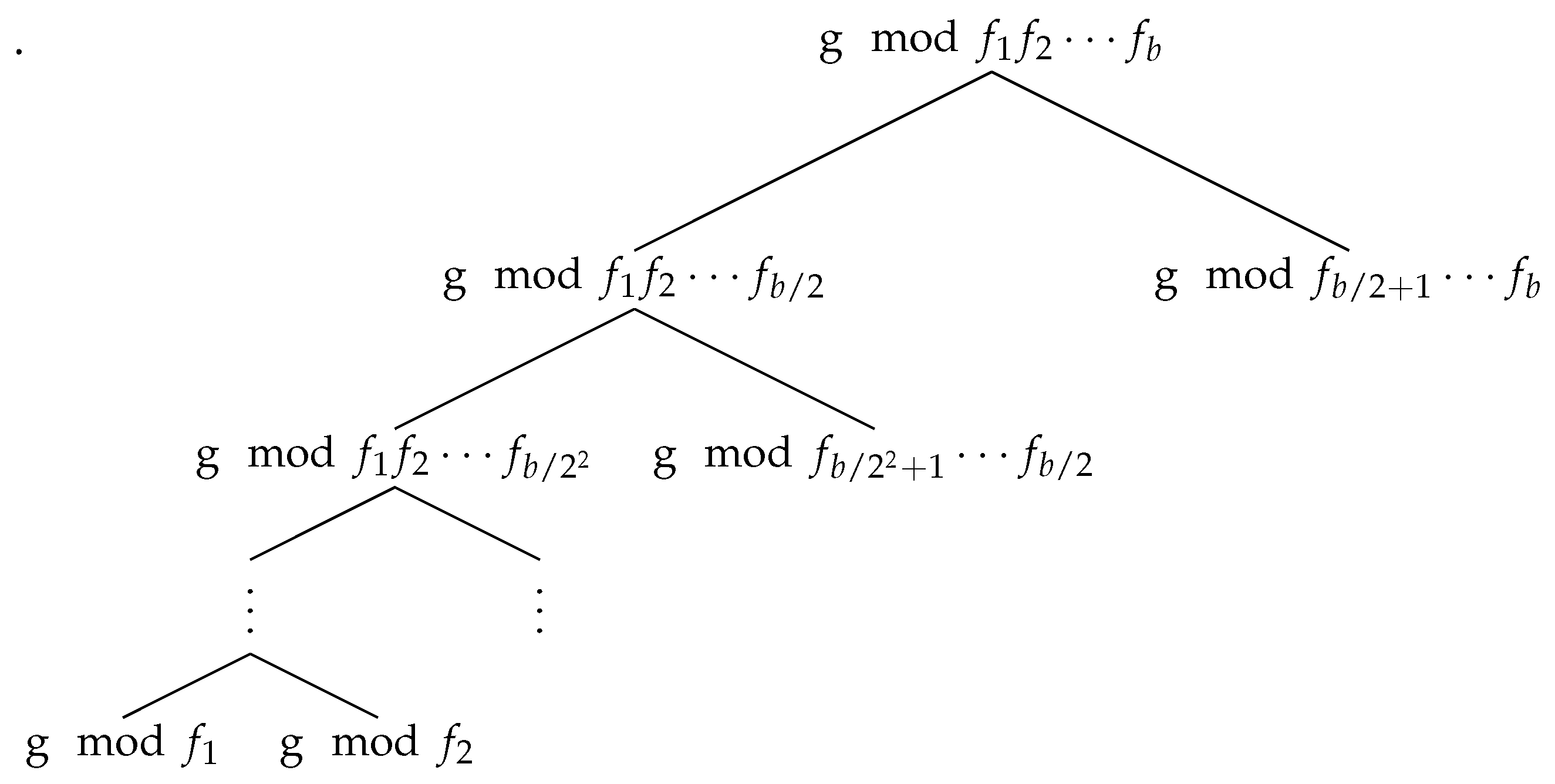
Figure 4.
Speedup factors of timings of the joint cost KPS-Parallel + xISOG-Parallel + 2xEVAL-Parallel over for each odd prime degree . Experimental timings correspond to an average of 100 runs, whereas the expected savings are obtained from the estimated number of field multiplications from (6) and (5).
Figure 4.
Speedup factors of timings of the joint cost KPS-Parallel + xISOG-Parallel + 2xEVAL-Parallel over for each odd prime degree . Experimental timings correspond to an average of 100 runs, whereas the expected savings are obtained from the estimated number of field multiplications from (6) and (5).
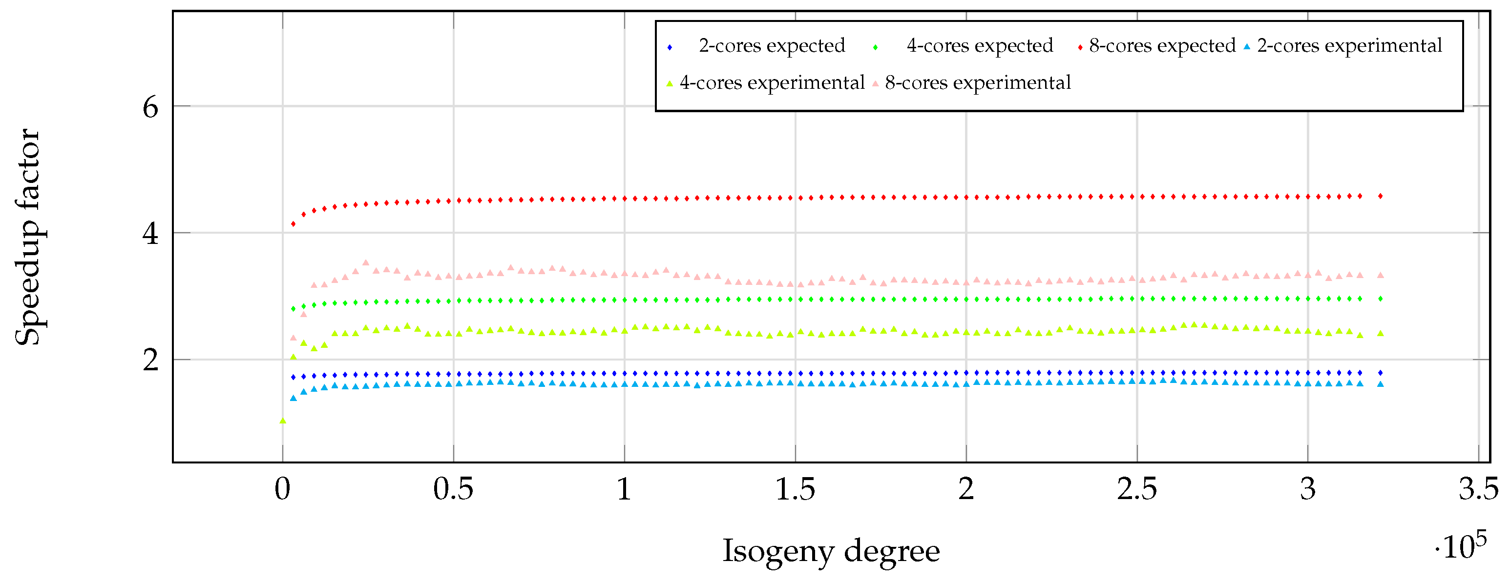

Table 1.
Aggregate computational time (in gigacycles) measured for the single-core square-root Vélu procedures KPS, xISOG, and xEVAL described in §Section 2.1, and of the two-core and four-core implementations of the parallel analogues described in §Section 3.2. The costs are summed over each odd prime degree , and the Total column corresponds to KPS + xISOG + 2xEVAL. Timings correspond with the average of 100 runs. (Gcc) is the number of gigacycles and (SF) is the experimental speedup factor considering the single core implementation as a baseline.
Table 1.
Aggregate computational time (in gigacycles) measured for the single-core square-root Vélu procedures KPS, xISOG, and xEVAL described in §Section 2.1, and of the two-core and four-core implementations of the parallel analogues described in §Section 3.2. The costs are summed over each odd prime degree , and the Total column corresponds to KPS + xISOG + 2xEVAL. Timings correspond with the average of 100 runs. (Gcc) is the number of gigacycles and (SF) is the experimental speedup factor considering the single core implementation as a baseline.
| Algorithm | Single core | Algorithm | Two cores | Four cores | ||
|---|---|---|---|---|---|---|
| Gcc | Gcc | SF | Gcc | SF | ||
| KPS | 23.6 | KPS-Parallel | 19.2 | 1.23 | 16.6 | 1.42 |
| xISOG | 58.5 | xISOG-Parallel | 34.5 | 1.70 | 25.8 | 2.27 |
| xEVAL | 59.5 | xEVAL-Parallel | 31.0 | 1.92 | 19.7 | 3.02 |
| Total | 201.1 | 115.7 | 1.74 | 81.8 | 2.46 | |
1One gigacycle is one billion clock cycles.
Disclaimer/Publisher’s Note: The statements, opinions and data contained in all publications are solely those of the individual author(s) and contributor(s) and not of MDPI and/or the editor(s). MDPI and/or the editor(s) disclaim responsibility for any injury to people or property resulting from any ideas, methods, instructions or products referred to in the content. |
© 2024 by the authors. Licensee MDPI, Basel, Switzerland. This article is an open access article distributed under the terms and conditions of the Creative Commons Attribution (CC BY) license (http://creativecommons.org/licenses/by/4.0/).
Copyright: This open access article is published under a Creative Commons CC BY 4.0 license, which permit the free download, distribution, and reuse, provided that the author and preprint are cited in any reuse.