

Submitted:
16 January 2024
Posted:
16 January 2024
You are already at the latest version
Abstract
Memristors are state-of-the-art, nano-sized, two-terminal, passive electronic elements with very good switching and memory characteristics. Owing to their very low power usage and a good compatibility to the existing CMOS ultra-high-density integrated circuits and chips, they are po-tentially applicable in artificial and spiking neural networks, memory arrays, and many other de-vices and circuits for artificial intelligence. In this paper, a complete electronic realization of ana-log circuit model of modified neural net with memristor-based synapses and transfer function with memristors and MOS transistors in LTSPICE is offered. Each synaptic weight is realized by only one memristor, providing enormously reduced circuit complexity. The summing and scaling implementation is founded on op-amps and memristors. The logarithmic-sigmoidal activation function is based on a simple scheme with MOS transistors and memristors. The functioning of the suggested memristor-based neural network for pulse input signals is evaluated both analytically in MATLAB-SIMULINK and in LTSPICE environment. The obtained results are compared one to another and are successfully verified. The realized memristor-based neural network is an im-portant step towards the forthcoming design of complex memristor-based neural networks for ar-tificial intelligence, for implementation in very high-density integrated circuits and chips.
Keywords:
memristor neural network
; logarithmic-sigmoidal transfer function
; artificial intelligence
; metal-oxide memristors
; memristor modeling
; LTSPICE models
1. Introduction
Artificial neural networks have inspiration from electro-chemical communication between neural cells in human brain and other biological neural systems [1,2]. Their applications have revealed power efficiency and promising utilization in very low-energy and mobile electronic schemes and devices [3,4]. Neuromorphic integrated chips have the ability to perform complex computations quickly and effectively, consuming minimal electric power [5,6,7]. In the past, Metal Oxide Semiconductor (MOS) transistor-based neural nets and optical neural networks were a leading approach for realizing analog neural nets, utilizing light, instead of electrical pulses to conduct neural computing, image and video processing, and other applicable tasks [8,9,10]. Some of the state-of-the-art improvements in this field are the neural nets based on memristors [11,12,13,14], which are generally used in the synaptic bonds for storing the synaptic weights [15,16,17].
Memristors predicted by Leon Chua [18] are electronic passive components with two electrodes, that have the ability to store electric charges, passed through their structure [19,20]. By applying electric pulses – voltage or current with definite amplitudes and durations, the resistance of memristors (also known as a memristance) could be altered. The memristors could work as tunable electronic resistors [21,22]. The first material memristor based on titanium dioxide (TiO2), is created in Hewlett-Packard scientific and research labs by Stanley Williams and his collaborators [21,23,24]. Different metal oxides, such as HfO2, Ta2O5, Nb2O5, and many others substances are utilized for realizations of memristor elements [25,26]. Some valuable properties of memristors are their low energy usage, very good switching and memory properties, high switching speed, nano-sizes and a good compatibility to the present-day Complementary MOS (CMOS) integrated chips and circuits [27,28]. Memristors are potentially applicable in memory matrices, reconfigurable analog and digital circuits, neural nets, and many others [29,30]. They are related to storage and computing in a single electronic circuit element [31].
Several different categories of memristor-based synapses, artificial neurons and neural networks are accessible in the related scientific works [32,33]. Some electronic synapses based on single memristor elements [7] and MOS transistors ensure only positive weights, which is a weakness of such realizations. More complicated schematics employ multiple memristors for each synapse [9], arranged in anti-parallel and bridge circuits. Such configurations enable realization of positive, zero, and negative synaptic weights [9,12]. An arrangement containing five memristors and electronic switches forms a π-type memristor synapse [13]. Certain synapses within this category utilize operational amplifiers (op-amps) and metal-oxide-semiconductor (MOS) transistors as differential amplifiers [14]. In contrast to the advantage of realization of positive and negative weights, the main drawback lies in the higher number of memristors per single synapse. For synapse realization, usually three or more memristors are used, and several op-amps are included [15]. A possibility to realize each synaptic weight with just a single memristor is available, which could significantly reduce neural circuit complexity [34,35].
For analysis and simulation of memristor-based neurons and neural networks with a large number of memristors, fast-operating and simple SPICE models of memristors and MOS transistors are desirable, for simplification the analyses and for decreasing the simulation time [36,37]. For this aim, a modified, enhanced and simplified SPICE model of metal-oxide memristors with activation thresholds is utilized [35]. Along with the software products of the Simulation Program with Integrated Circuits Emphasis (SPICE) family, the used here LTSPICE simulator is a preferred one, owing to its user-friendly interface, free license, an absence of artificial restrictions on the maximal number of the considered electronic elements and their connections, and very good convergence characteristics [33]. Owing to its benefits LTSPICE product is applied for the electronic simulations in the present work. For comparison and confirmation of the derived results, MATLAB, Simulink and Neural Network Toolbox [32] are also utilized.
After a comprehensive reference investigation, it was established that complete circuits of memristor-based synaptic schemes, neurons, transfer functions and neural nets, and related programming codes and results, together with comparisons are not represented in the available scientific papers. It is also known that some issues with realization of negative synaptic weights are reported [6]. This was the main motivation for proposing the implementation of a memristor-based neural network in LTSPICE, as the activation function was realized with a voltage-controlled voltage source in LTSPICE simulator [34]. Subsequently a single neuron with activation function implemented with memristors and MOS transistors is also realized and proposed to the readers [35].
The goal of this paper is realization of a whole electronic implementation of a memristor neural network in LTSPICE environment. To achieve this purpose the following tasks are placed: realization of a new electronic circuit based on memristor and MOS transistors, realizing a logarithmic-sigmoidal transfer function; realization of a simple adder based on memristors and operational amplifiers with minimal number of elements; synthesis and analysis of a simple multi-layer neural network, utilizing memristors for the synaptic weights of positive and negative signs, and to employ a minimal number of electronic components in LTSPICE environment [33]. An artificial neuron with two distinct inputs for the positive and for the negative synaptic weights is implemented by employing memristor elements and operational amplifiers. Single metal-oxide memristors are used to implement the synapses of the considered neural network. For the analyses and simulations, a simple, fast-operating and accurate LTSPICE memristor model with activation threshold is applied [35]. In this paper, the opportunity to implement memristor-based neural network circuits and to make analyses and comparisons between different realizations of neural nets in SPICE simulators is proposed to the readers. Future work on the subject is predicted, considering synthesis and analysis of more complex multi-layer memristor-based neural networks, as well as their practical implementation and comparison with other proposed realizations.
The paper is organized as follows. Section 2 presents memristors, their modeling, tuning and a brief comparison between memristor models. The LTSPICE realization and analysis of the applied memristor model is considered in Section 3. The considered simple and fast-operating LTSPICE memristor neuron is discussed in Section 4. The applied activation function based on memristors and MOS transistors is presented in Section 5. Section 6 presents the offered simple neural network with memristors and MOS transistors. Section 7 presents the derived results in MATLAB, SIMULINK and LTSPICE and their comparison. The conclusion shown in Section 8 summarizes the results and proposes future work on the topic.
2. Memristors - Modeling, Tuning, Comparison, and the Applied Memristor Model
For improvement and understanding the main conception of the work, according to the structure, operation, modeling, tuning and comparison of metal-oxide memristors [36,37], a short overview of the basic aspects of memristors is first presented.
2.1. A short depiction of memristor elements and their operation
The memristors are passive one-port electronic elements with memory and switching properties. In the scientific reports, a lot of memristors based on different materials, as metal-oxides, polymeric, ferroelectric, spintronic and others are described [17,18,19,20,21,22,23,24]. Metal-oxide memristors have a central position in the family of memristors, owing to their stable characteristics and parameters, very good switching and memorizing properties [24]. A part of the memristor nanostructure is doped by oxygen vacancies, applying electroforming processes [18]. The memory and switching effects in memristors depend on their ability to undergo alterations of their resistance, proportional to their state variable, when voltage or current signals are applied [19]. The state variable of a memristor x indicates the ratio between the lengths of the doped layer and the whole memristor structure. The memristor has two limiting values of its resistance, usually denoted as RON (the ON-resistance state) and ROFF (the OFF-resistance state).
The behavior of memristors in electric field is quite different, in comparison to those of the classical electronic passive elements – the resistor, inductor and capacitor. Owing to its specifics modeling of memristors is mandatory for its analysis by electronic simulators and applications in electronic schemes and devices [19,26].
2.2. The Process of Modeling of Memristors [19,24,30]
Each mathematical model of a memristor is built on two key equations [26]. The first one offers the i-v relation, and the second one connects the time derivative of state variable x and the memristor current i (or the memristor voltage v). A large collection of repeatedly used metal-oxide memristor models, enclosing these of Williams-Strukov [18], Joglekar [22] and Biolek [23] is represented by the next general set of equations (1) [26]:
where i and v are the memristor current and voltage, M is the so-called memristance (the state-dependent resistance of the memristor), x is the state variable of the memristive element, k is a constant which is dependent on the main physical parameters of the element – the ionic drift mobility µ, the ON-state resistance and the whole length D. The expression f(x) is a window function, utilized for limitation of the state variable in the interval from 0 to 1 and for introducing the boundary effects at a hard-switching mode [26]. Strukov-Williams memristor model [18] is described by the next set of equations (2):
where RON and ROFF are minimal and maximal values of the memristance, and fSW(x) is a simple and low-order polynomial window function proposed by Williams and Strukov [18]. This classical memristor model is a very simple one, and owing to the reduced number of the elementary mathematical operations it has a very high operating speed []. Owing to the linear dependence between the time derivative of the state variable dx/dt and the memristor current i, this model could not express the different behavior of the memristors for voltages, lower or higher than one volt [21,26]. The window function is related to the so called terminal state problems [20,31]. This memristor model has a comparatively low accuracy in simulation of complex and non-symmetrical experimental current-voltage characteristics of metal-oxide memristors. Joglekar memristor model is one of the widely-used metal-oxide memristor models [22] and it is presented by the following system (3):
where fJ (x) is a polynomial window, proposed by Joglekar and Wolf [22]. This traditional model for metal-oxide memristors is a simple one, and it has a comparatively high functioning speed [24,31]. Due to the linear relation between the time derivative of state variable x and the current, this model fails to capture the distinct behavior of memristors under voltages lower or higher than one volt. Terminal state problems are related to the applied window function [22,24]. The used polynomial window function is adjustable one and ensures different slope, according to the parameter p and the memristor state variable.
Biolek model for metal-oxide memristors, which is one of the mainly-utilized standard memristor models, is presented by the next system (4) [23]:
where fB (x,i) is a window function, proposed by Biolek, and p is a positive integer [23]. This classic model is comparatively simple and fast-operating one [24,30]. The window function correctly represents the boundary effects and is not related to terminal state issues [24]. This classical memristor model has a comparatively good accuracy in modeling of experimental current-voltage relationships.
Lehtonen-Laiho memristor model is a classic one, frequently applied for modeling of metal-oxide memristors, and is expressed by the next set of equations (5) [21]:
where m and n are integer coefficients, and γ, α, β, and χ are coefficients for tuning the memristor model [21]. This model is a relatively complex one and has a high operating rate []. Due to the highly nonlinear relation between time derivative of state variable x and the memristor voltage, this standard model correctly expresses the different behavior of metal-oxide memristors for signals, higher or lower than 1 V [21]. Usually, in this memristor model, the classical Biolek window is applied [24,31]. This model has a high accuracy.
The applied in the present analyses modified memristor model, denoted by A14mod [35], is based on Joglekar memristor model and Lehtonen-Laiho model using the Hann window function sin2(πx) [24,35]. The model has an activation threshold vthr, applied in the state differential equation, using the standard Heaviside step function [23]. This modified memristor model is presented by the next set of equations (6) [35]:
where k is a constant dependent on the physical parameters of the memristor nanostructure and m is an odd and integer exponent [35]. This modified memristor model has a simple mathematical structure, the applied Hann window function is not related to terminal state problems. If the voltage is lower than the activation threshold vthr, then the time derivative of the state variable is zero and the memristor behaves as a simple and linear resistor with a constant conductance [24,26]. This mode is used for the operation of metal-oxide memristors in adjusted neural networks after finishing the training processes and establishing constant values of the synaptic weights [24]. The modified memristor model A14 mod is a simple one, with a high operating speed and a good accuracy, and it is very appropriate for application in neural networks.
2.3. Fine adjustment and parameter estimation of the applied memristor model [24,31,32]
In this work, we analyse the considered modified model of a memristor based on metal oxides [35] and it is fully allocated by equation (6). This memristor model incorporates multiple parameters that allow its precise and fine-tuning process. In [35], this modified memristor model is tuned according to experimental data of metal-oxide memristors [20]. In this work, it is adjusted in accordance with current-voltage dependencies, derived by experimental data of Knowm self-directed channel memristors [36]. A technique for altering the model’s parameters till reaching the complete minimum of the Root Mean Square (RMS) error between the simulated and the experimental current of the memristor is applied [32]. Many scientists utilize simulated annealing and gradient descent algorithms for reaching the optimal values of the parameters of the memristor models [24,32]. The applied model is simple and applicable for simulations of memristor-based circuits and devices.
MATLAB-SIMULINK environment is utilized to extract the parameters from the considered memristor model [32]. The optimization approach for tuning the metal oxide memristor model involves modifying the coefficients and looking for the global minimum of the root mean square (RMS) error between the experimental and simulated current-voltage (i-v) characteristics. At each iteration step one of the coefficients of the model is altering by a small growth [32]. The RMS error between simulated and experimental i-v relations is computed. The other parameters of the model are also changing. After finalizing the tuning procedure, a graphical evaluation of the obtained current-voltage relationship and its nearness to the experimental one is also realized, paying attention on the form of the derived i-v pinched hysteresis loop and especially on the intervals of switching the resistance of the memristor element. The respective time diagrams of simulated and experimental memristor currents are also compared. An important condition for finalizing the adjustment process is minimization of RMS error [32]. Extra simulations are conducted for obtaining the optimal model’s coefficients, applying smaller increments for their alterations [32]. The precise values of memristor model’s parameters are also obtained, using the least squares method in MATLAB, applying Optimization Toolbox [32]. The parameter estimation process could be summarized in several main steps:
- Determination the value of root mean square error (RMSE) for stopping the estimation process, the corresponding deviations and the number of maximum iteration steps;
- Starting simulation and computing the current of the memristor element according to the applied modified memristor model;
- Evaluation of the RMS error (the cost function) between the calculated and experimental currents of the considered memristor;
- Alteration of model’s parameters according to a gradient descent of RMS error;
- When the determined RMS error is reached, or the maximal number of iteration steps are realized, the simulation process and evaluation of the derived model’s parameters are finished. The voltage signals in MATLAB-Simulink memristor model are previously sampled, the time step is with a value of 10 µs. The experimental memristor current is represented by imes. The output of the Simulink memristor model is related to the simulated current of the memory element icalc. The cost function Scost is an algebraic sum of the squared differences between the experimental and calculated currents – eq. (7) [24,32]:
The type of the applied memristor model is important for training the networks and adjustment of the synaptic weights of memristor-based neural networks by short voltage pulses. In the next section the generation and analysis of LTSPICE memristor model, corresponding to the considered modified memristor model, its main characteristics and properties are discussed.
3. LTSPICE Library Model [35] and analysis of the applied Memristor model
The main idea, utilized for construction of the LTSPICE [33] memristor library model, is to build a simple and fast-operating equivalent circuit, corresponding to (6). Before realization of the current-voltage characteristics, the derivation of the state variable x is needed. The memristor state variable is obtained by integration of the state differential equation with respect to time. This process is ensured by a capacitor; its current is set to be proportional to the time derivative of the state variable x [26,31]. The current of the capacitor is generated by a voltage-controlled current source, according to the left-hand side of the state equation in (6). The initial voltage of the integrating capacitor is set to be equal to the starting value of the memristor state variable. The voltage across the integrating capacitor is directly proportional to the state variable in each moment in the time domain. To avoid rapid changes of the voltage across the capacitor, which could lead to convergence issues, a high-valued resistor could be attached in parallel to the capacitor [31,36]. Additional voltage-controlled current source is generating the memristor current, according to the right-hand side of the first equation in (6). The initial row of the LTSPICE code displays the memristor model identifier, indicated as A14mod. The memristor terminals are denoted as top electrode (te) and bottom electrode (be). The optional terminal Y is utilized for measuring the memristor state variable. The parameters of the model - RON, ROFF, k, m, mm, m0 and vthr are presented in the next row. The coefficient m0 represents the initial value of the memristance. The integrating capacitor is connected between the terminal Y and the ground electrode. Its capacitance is 1000 mF. The initial voltage of integrating element C1, denoted as “.IC”, is expressed by the first equation of (6) [35]. It is inversely proportional to the starting value of the memristance. The fifth row represents the additional resistor Rad with a value of 100 GΩ, connected in parallel to C1 and utilized for a partial avoidance of convergence problems. The dependent source G2 presented in the sixth row expresses the time derivative of the state variable x.
The controlled source G1 expresses the current of the memristor element. In row 8, a differentiable and flat step-like function is presented. It is utilized for realization of the state equation, containing the memristor activation threshold vthr. The code, presented below is finished with the command “ends” [26,33,35].
- 1
- .subckt A14mod te be Y
- 2
- .params ron=100 roff=25e3 m0=300 k=10e4 m=5 vthr=0.2 mm=1e-24
- 3
- C1 Y 0 {1}
- 4
- .IC V(Y)={(m0-roff)/(ron-roff)}
- 5
- R1 Y 0 100G
- 6
-
G2 0 Y value={((k*pow(V(te,be),m))*((pow(sin(pi*V(Y)),2)))*(stpp((vthr-abs(V(te,be))),mm)))}
- 7
- G1 te be value={V(te,be)*((1/(ron*(V(Y))+roff*(1-V(Y)))))}
- 8
- .func stpp(x,p)={0.5*(1+(x/sqrt(pow(x,2)+p)))}
- 9
- .ends A14mod
The parameter mm determines the sharpness of the step-like function stpp. For a quick and easier tuning of the initial value of the memristance m0, the state variable of the memristor in the initial moment is expressed as a function of m0 in the fourth row. After selecting the memristor model A14mod in LTSPICE and placing on the plotting field, right-click on the memristor, in the SPICE row of the appeared window, write m0=300, then place a tick in the right by double left mouse button click, to make m0 visible and confirm by clicking OK. The considered LTSPICE code is included in a unified memristor model library, freely available for use and download at https://github.com/mladenovvaleri/Advanced-Memristor-Modeling-in-LTSpise [31]. This library contains many LTSPICE models of memristors and memristor-based electronic circuits, available for use and comparisons. The considered modified memristor model is analyzed with pulse and sine signals at a constant amplitude of 1.1 V and for different frequencies. In Figure 3a, the testing circuit for memristor analysis is presented for its visual observation. In the present case, the additional electrode Y is not included for simplification of the electronic circuitry. The initial value of the memristance is set to be 5 kOhms. After obtaining the i-v relationships of the memristor model for sinusoidal signals with amplitude of 1.1 V and different frequencies (100 kHz, 1 MHz and 10 MHz) in LTSPICE environment, they are presented in Figure 3b–d for their visual comparison and for confirmation of the correct operation of the modified memristor model. It is visible that, when the signal’s frequency increases, then the surface of the i-v loop decreases in accordance with the basic memristors’ properties and fingerprints [24,30].
Memristors, participating as synaptic weights, are tuned during the neural network training by positive or negative voltage pulses with a level, which absolute value is higher than the activation threshold vthr [35]. An example of synaptic weight adjustment is presented in Figure 4. A simple electronic circuit, containing a pulse voltage source and a memristor, represented by the modified model A14mod, is shown in Figure 4a for a visual expression of its structure and operation. The voltage source generates a sequence of rectangular and positive pulses with a duration of 1 ns and a duty cycle of 50 %. The amplitude of the voltage is 1.1 V. Figure 4b represents the time diagrams of the pulse voltage signal and the corresponding change of the memristance M in LTSPICE. In this case the initial value of the memristance is M1 = 10 kOhm, which corresponds to a synaptic weight of w1 = 1. The final value of M2 = 9 kOhm corresponds to a synaptic weight of w2=1.1111. In this case, the change of memristance with ∆M = 1 kOhm corresponds to alteration of the synaptic weight with ∆w = 0.1111. The needed time interval for this memristance change, together with the pauses between the impulses, is about 28 ns. The effective duration of the voltage pulses for this time interval is about 14 ns. Figure 4c represents the results, derived by a simulation in MATLAB, which have a very good coincidence to Figure 4b and confirms the tuning process.
This result will be also mathematically confirmed by integration of the state differential equation of system (6), modified and represented here by (8):
In eq. (8), because the used voltage pulses are higher than the activation threshold vthr, in the right hand side, the step function “stp” is missed. Equation (8) is transformed to (9), where the state variable x and the time variable t are separated one to another:
According to the current-voltage relationship in system (6), the state variable x is expressed as a function of the memristance M by the next eq. (10):
Equation (9) is integrated between x1 = 0.8251, corresponding to M1 = 10 kOhm, and x2 = 0.8427, related to M2 = 9 kOhm, using (10), and the following eq. (11) is obtained:
Then, the effective duration of the applied pulses (a single pulse or a sequence of short impulses) is obtained as follows – formula (12):
The obtained time for synaptic weight adjustment corresponds to the derived simulation result and confirms the proper tuning the memristance by pulses. Another simulation is conducted with negative voltage pulses and the same circuit shown in Figure 4a is used. The respective time diagram of the applied negative pulses and the corresponding memristance alteration in LTSPICE is presented in Figure 5a. Figure 5b represents the results, derived from analysis in MATLAB, which is in a good agreement with Figure 5b and confirms the correctness of the adjustment process. The analysis starts with initial value of the memristance, equal to M1 = 5 kOhms, related to a synaptic weight of w1 = 2 and a state variable of x1 = 0.9129. The final value of the memristance M2 is 6 kOhms, corresponding to a synaptic weight with a value of w2 = 1.6667 and a state variable x2 = 0.8954. The change of the memristance with 1 kOhm in this case corresponds to alteration of synaptic weight with ∆w = 1.6667-2= - 0.3333. The effective duration of the pulse is about 79ns/2 = 39.5 ns.
The analytical confirmation of this result is as follows – formula (13):
For the future practical implementation of memristor-based synapses, the tuning process will be related to a measurement of the achieved memristance, until reaching the needed resistance and stopping the pulse sequence. According to the requirement for a quick change of the memristance and the corresponding synaptic weight, the applied modified memristor model A14mod ensures a rapid alteration of the state variable and the memristance at applied voltage pulses. Its simple structure and low simulation time ensures the generation and analysis of complex neural networks with a high number of memristors in LTSPICE environment. Additional comparison of the applied memristor models, according to simulation time is conducted for two cases – decreasing and increasing of memristance, according to the analyses shown in Figure 4 and Figure 5. The results presented in Table 2 express the faster operation of the applied modified model, according to Lehtonen-Laiho model. The simulations were conducted on a computer with 8 GB RAM, i5 Intel processor, and Microsoft Windows 10 Pro operating system. According to Joglekar and Biolek models, the modified model A14mod has comparable simulation time and better switching properties.
4. Memristor-based Transfer Function
The considered realization of a logarithmic-sigmoidal activation function is presented in Figure 6a for its visual expression and for further discussion. The considered transfer (activation) function is realized by two MOS transistors M1 and M2, connected in anti-parallel, the memristor U1 and a DC voltage source V2 [35]. The MOS transistors are of N-type and in the present case, they are chosen to be Si7540DP_N, using the standard LTSPICE library [33]. The transistors are connected as diodes and their gate and source terminals are directly attached one to another. The anti-parallel connection of the MOS transistors ensures a symmetrical transfer function. The memristor U1 is connected in series to the MOS transistors. Its voltage drop is the difference between the input and the output signals. The voltage source V2 ensures shifting of the output signal [35]. The dependence between the output and input voltage signals is very similar to a logarithmic-sigmoidal function, presented by the following expression (14):
For determination of the optimal value of the coefficient k, several different experiments and comparisons are conducted with the use of the dependent voltage source B1 shown in Figure 6b, which voltage represents a logarithmic-sigmoidal activation function. It is established that for k = 5 and m0 = 150 Ohms, the best proximity between the transfer functions is realized. The expression of the voltage of the behavioral source B1 is vtf = 1/(1+exp(-5*vin_tf)).
The n-channel MOS transistor Si7540DP_N used in this paper has a simpler construction, lower drain-source voltage, lower drain current, and higher speed compared to the Si4864DY transistor [35]. The activation functions depicted in Figure 7 correspond to the circuits illustrated in Figure 6. These graphics are presented for their visual expression and comparison of their proximity. The transfer function of the MOS transistor-based schematic is represented by the black curve, while the theoretical activation function is depicted by the blue curve. After several experiments with different values of the coefficient k, a very good proximity between the considered transfer functions is established when the coefficient in the theoretical expression is k = 5. In the next section, an artificial neuron, based on memristors is discussed.
5. Memristor-based Neuron [35]
Figure 8 presents a block diagram of a neuron and illustrates the structure and operation of a neuron based on memristors for further explanations and discussion [2,3]. The input signals of the neuron are represented as x1, x2, … and xN. The signals are directed to synapses based on memristors, with corresponding weights denoted as w1, w2, ..., and wN. A single memristor is employed for each synapse, and its resistance determines the corresponding synaptic weight. The change of the respective synaptic weight is realized by alteration of the corresponding memristance with externally applied voltage or current pulses. The signals obtained after the memristor synapses are directed to an adder, implemented by the use of operational amplifiers and memristors, operating as linear and constant resistors [34,35]. The signal derived after the adder is represented as y_in. This signal is directed to a log-sigmoidal transfer function, constructed by metal-oxide memristors and MOS transistors [35]. The output signal of the artificial neuron is indicated by y.
The functioning of the memristor-based neuron under consideration is related to a feed-forward and back-error propagation learning algorithm [3]. Various activation functions could be utilized after the adder [3,7]. Commonly utilized in the neural networks are smooth and differentiable transfer functions, such as logarithmic-sigmoidal and tangent-sigmoidal ones [7]. The relay activation function, also known as the standard Heaviside function, is also utilized in artificial neural nets [3]. A gain factor can also be utilized to apply a linear activation function in artificial neurons. Figure 9 illustrates a principal schematic of the considered artificial neuron based on memristors providing a description of its structure and operation. The input signals x1 – x6 are normalized in the interval between -0.1 and +0.1 volts, in order to avoid alteration of the resistances of the synaptic weights during the application of the adjusted neural network. The number of the memristors, realizing the synaptic weights could vary, according to the needed inputs of the artificial neuron. The synaptic weights are presented by the metal-oxide memristors M1 – M6. The memristors M1, M2 and M3 are related to negative weights, while the other memristors - M4, M5 and M6 are placed for realization of the positive synaptic weights. The considered synapses are connected to the inverting inputs of the op-amps OA1 and OA2, respectively. The memristors M7 and M9 are applied for realization of voltage feedbacks of the respective op-amps. The output signal of the op-amp OA2 is directed to the inverting input of op-amp OA1 via the memristor element M8. The non-inverting inputs of the operational amplifiers are connected to the ground [34,35]. The feedback memristors M7, M8 and M9 are adjusted to a memristance of 10 kOhms.
Using Kirchhoff’s laws, the output signal of op-amp 1, correspondent to the signal y_in, is derived as follows – formula (15):
Having in mind that M7 = M8 = M9 = 10 kΩ, the next expression (16) is derived after algebraic processing of formula (15):
where the coefficients in front of the signals x1 – x6 are the corresponding synaptic weights - formula (17) [34,35]:
Observably, synaptic weights w1, w2, and w3 are with negative values, whereas the weights from w4, w5 and w6 are positive.
Figure 10 illustrates the implementation of the considered memristor neuron in LTSPICE environment, providing further details and discussions. It is associated with the electronic circuit presented in Figure 11. The presented pulse voltage sources V1, V2, V7, V8, V9 and V37 are corresponding to the signals x1 – x6 and they generate the input signals – vin1, vin2, vin3, vin4, vin5 and vbias. The adder has two inputs – for negative and for positive synaptic weights, which are denoted by minus and plus, respectively [35]. The output electrode of the adder is denoted by “summ”. The structure of the log-sigmoidal transfer function corresponds to Figure 6a. A detailed realization of the adder in LTSPICE simulator is presented in Figure 11 for its description and further explanations. The op-amps U1 and U2 are power supplied by two DC voltage sources of 3 Volts. Sometimes, the voltage across the feedback memristors could exceed the activation threshold of the applied metal-oxide memristors [35]. The feedback voltage depends on the output signal y_in, which is proportional to the weighted sum of the input signals. To avoid the respective voltages across the feedback memristors to exceed the memristor activation threshold, the voltage feedback elements M7, M8 and M9 are substituted by memristor-based blocks, enclosing two memristors connected in a series connection [35].
The exact number of memristor elements n in a block, realizing a feedback element could be calculated, using the absolute value of the output signal vsumm=y_in (in Figure 9), divided by the activation threshold vthr, and applying the truncation function “ceil”, which returns the smallest integer, not less than its argument – formula (18):
The signal after the adder vsumm is connected to a memristor-based voltage divider and a buffer amplifier, presented in Figure 12. The transfer coefficient of the voltage divider is 0.1. This divider is needed for ensuring the normal operation of the memristor-based synapses of the next layer of the neural network [34,35], which voltage should not exceed the activation threshold vthr.
The element U46 has a constant resistance of 1777.78 Ohms and is realized by only one memristor, while the number of the other memristors in the voltage divider is determined by the next formula (19), to ensure that the voltage drop across the memristors does not exceed the activation threshold vthr:
Sometimes, the normal operation of the memristors in the voltage divider could be violated, owing to the connected synapses of the next layer of the neural network. To ensure their normal functioning without exceeding the activation threshold and to avoid functioning in a soft-switching mode, a buffer amplifier is connected after the voltage divider. It is based on non-inverting operational amplifier.
6. Memristor-Based NN with TF, realized with MOS transistors
The block diagram of the memristor-based neural network under analysis is presented in Figure 13 for its visual expression and further comments on their structure and operation. It contains five input nodes for applying the input signals x1 – x5. The hidden layer of the neural network contains four neurons – N1, N2, N3 and N4. The bias signals are denoted by b1, b2, b3 and b4. The synaptic weights are denoted by wij, where i = 1 - 5 is the number of the neuron, and j is the number of the input signal. The adders are used for summing the weighted input signals. The output signals of the adders are denoted by s1, s2, s3 and s4. These signals are applied to the logarithmic-sigmoidal activation functions tf1, tf2, tf3 and tf4, respectively. The described elements form the hidden layer of the considered neural network. The signals tf1, tf2, tf3 and tf4 are applied to the output layer of the neural network, which contain two neurons – Nout1 and Nout2. The synaptic weights are denoted by vkp, where k is the number of the neuron, and p is the number of the respective input signal. The bias signals of the adders are denoted by bout1 and bout2. The output signals of the adders are denoted by s1out and s2out. The applied transfer functions tfout1 and tfout2 are of type “purelin” []. They are realized with buffer amplifiers, using op-amps. The output signals of the neural network are denoted by y1 and y2.
The operation of the presented memristor-based neural network is based on its training in MATLAB environment, using feed-forward and back-error propagation algorithm, for adjustment of the synaptic weights [3,32]. The obtained values of the weights are used for tuning the memristances and to create the neural network in LTSPICE environment, which will be discussed in the next section.
The input signals are sequences of rectangular voltage pulses. The pulse duration is 0.8 ms. The duty cycle is 50 %. The levels of the input and the bias voltage signals are shown in Table 3 for their visual evaluation. The bias signal is set to 100 mV and does not exceed the memristor activation threshold vthr.
The synaptic weights for the hidden layer of the neural network are presented in Table 4 for their evaluation and for further discussion.
The corresponding resistances of the single-memristor synapses are denoted by M1 – M5 and are presented in Table 5. Their values are obtained using formula (11). Having in mind that the bias signal is vbias = 0.1 V, instead of 1 V, the value of the memristance Mbias is obtained by multiplication with 10.
The synaptic weights of the synapses in the output layer are presented in Table 6.
The memristances, corresponding to the synaptic weights for the output layer are represented in Table 7.
A principal schematic of the considered memristor-based neural network is illustrated in Figure 14. The input signals are denoted by x1 – x5, the bias signal is denoted by b. This schematic corresponds to the block diagram, presented in Figure 13. The electronic realization of the considered neural network in LTSPICE simulator, corresponding to the block diagram of Figure 13 and to the principal schematic presented in Figure 14, is given in Figure 15. It is presented for a visual observation and realization by the readers in similar SPICE simulators. The circuits is also available at: https://github.com/mladenovvaleri/Advanced-Memristor-Modeling-in-LTSpise [31]. Figure 16а illustrates the time diagrams of the input signals and the bias signal, giving their visual representation. The signals after the adders are presented in Figure 16b. Figure 16c represents the signals after the logarithmic-sigmoidal transfer functions and Figure 16d illustrates the output signals of the neural network in LTSPICE environment. The considered neural network is also realized in SIMULINK-MATLAB environment [32]. The SIMULINK schematic of the network is presented in Figure 17 for its visualization and further comments. The input signals are realized by pulse generators. They are forwarded to MATLAB workspace by the standard blocks “To workspace” for further analysis. The synaptic weights are corresponding to gain amplifiers, which zoomed diagram is given the right down corner of the schematic. The adders are realized by standard summing blocks. The logarithmic-sigmoidal and the linear transfer function is realized by “MATLAB function” blocks. The time step is 0.001 ms. The simulation time is 6 ms. The time diagrams, obtained by the function “plot” after finishing the simulation on MATLAB-SIMULINK environment are presented in Figure 18. The input signals x1 – x5 are represented in Figure 18a. The signals after the adders and after the transfer functions of the hidden layer are illustrated in Figure 18b. Figure 18c presents the output signals of the neural network.
The considered neural network is also simulated in MATLAB, using the neural network toolbox [32], for conducting a comparison of the results, derived in SIMULINK and in LTSPICE [33]. Table 8 compares the signals’ levels, derived in LTSPICE and MATLAB -Simulink [32]. Identical results are derived from the conducted analyses and simulations. This comparison confirms the capability of the considered memristor-based neural network and activation function to properly operate with pulse input signals with levels lower than the activation threshold of the applied metal-oxide memristors.
4. Discussion
Comparing the simulation results of the considered neural network, realized in LTSPICE, MATLAB and SIMULINK software, a very good matching of the signals after the adders, the transfer functions and the outputs is established. The maximal error between the output signal’s levels is less than 3 %. The synapses of the neural network are implemented with single memristors and operational amplifiers for summation, utilizing their inverting inputs. The suggested synapses implement both positive and negative weights. The logarithmic-sigmoidal activation function utilized in the research relies on a combination of a metal-oxide memristor and two MOS transistors, connected in anti-parallel. The analyses demonstrate a strong correlation between the obtained results, confirming the accurate functionality of the suggested memristor-based neural network.
5. Conclusions
The main purpose of this paper - realization of a complete electronic implementation of a memristor-based neural network in LTSPICE environment has been achieved. The related tasks are resolved – a modified logarithmic-sigmoidal transfer function, based on memristors and MOS transistors is realized; a simple adder, founded on memristors and operational amplifiers is realized with minimal number of electronic elements; a simple multi-layer artificial neural network, using memristors for the synaptic weights of positive and negative signs, employing minimal number of electronic components in LTSPICE environment is generated and analyzed. The analyses and simulations are performed, using MATLAB, SIMULINK and LTSPICE. We have applied A14mod memristor model, which is better than the existing ones (in terms of faster operation and simulation), which model helps for faster simulation when the synaptic weights are tuning, during the training of the neural network. The main advantage of the considered memristor-based artificial neural network is its simple realization with the use of very low-power and nano-sized metal-oxide memristor elements, with a very good compatibility to the present-day CMOS high density integrated electronic chips and circuits. This work introduces an opportunity for readers to explore implementations of neural network circuits, based on memristors. It encourages the analysis and comparison of various realizations of artificial neural networks, using SPICE simulators, together with practical measurements. The future work in this field will be related to exploration of synthesis and analysis of more complex multi-layer memristor-based neural networks for artificial intelligence. Additionally, it aims to explore into practical implementation of such neural networks and compare them with other similar proposed implementations.
Author Contributions
Conceptualization, V.M.; methodology, V.M.; software, V.M. and S.K.; validation, V.M. and S.K.; formal analysis, V.M.; investigation, V.M. and S.K.; resources, V.M. and S.K; data curation, V.M. and S.K; writing—original draft preparation, V.M. and S.K; writing—review and editing, V.M.; visualization, V.M. and S.K.; supervision, V.M.; project administration, V.M.; funding acquisition, V.M. All authors have read and agreed to the published version of the manuscript.
Funding
This research received no external funding.
Data Availability Statement
Not applicable.
Conflicts of Interest
The authors declare no conflict of interest.
References
- Wang, S.; Song, L.; Chen, W.; Wang, G.; Hao, E.; Li, C.; Hu, Y.; Pan, Y.; Nathan, A.; Hu, G.; Gao, S. Memristor-Based Intelligent Human-Like Neural Computing. Adv. Electron. Mater. 2023, 9, 1–39. [Google Scholar] [CrossRef]
- Sah, M.P.; Kim, H.; Chua, L.O. Brains Are Made of Memristors. IEEE Circuits Syst. Mag. 2014, 14, 12–36. [Google Scholar] [CrossRef]
- Aggarwal, C. Neural Networks and Deep Learning; Springer Int. Publ. AG: Berlin, Germany, 2018; ISBN 978-3-319-94463-0. [Google Scholar]
- Krestinskaya, O.; Salama, K.N.; James, A.P. Learning in Memristive Neural Network Architectures Using Analog Backpropagation Circuits. IEEE Trans. Circuits Syst. I Regul. Pap. 2018, 66, 719–732. [Google Scholar] [CrossRef]
- Bradley, W.M.D.; Mears, R.J. Backpropagation learning using positive weights for multilayer optoelectronic neural networks. In Proceedings of the Conference Proceedings LEOS'96 9th Annual Meeting IEEE Lasers and Electro-Optics Society, USA, 1996; Volume 1, pp. 294–295. [Google Scholar] [CrossRef]
- Parisien, C.; Anderson, C.H.; Eliasmith, C. Solving the problem of negative synaptic weights in cortical models. Neural Comput. 2008, 20, 1473–1494. [Google Scholar] [CrossRef]
- Xu, W.; Wang, J.; Yan, X. Advances in memristor-based neural networks. Front. Nanotechnol. 2021, 3, 645995. [Google Scholar] [CrossRef]
- Hong, Q.; Zhao, L.; Wang, X. Novel circuit designs of memristor synapse and neuron. Neurocomputing 2018, 330, 11–16. [Google Scholar] [CrossRef]
- Sah, M.P.; Yang, C.; Kim, H.; Chua, L. A voltage mode memristor bridge synaptic circuit with memristor emulators. Sensors 2012, 12, 3587–3604. [Google Scholar] [CrossRef]
- Dai, Y.; Feng, Z.; Wu, Z. A Novel Window Function Enables Memristor Model With High Efficiency Spiking Neural Network Applications. IEEE Trans. Electron Devices 2022, 69, 3667–3674. [Google Scholar] [CrossRef]
- Wen, S.; Xie, X.; Yan, Z.; Huang, T.; Zeng, Z. General memristor with applications in multilayer neural networks. Neural Netw. 2018, 103, 142–149. [Google Scholar] [CrossRef] [PubMed]
- Zhang, Y.; Wang, X.; Friedman, E.G. Memristor-Based Circuit Design for Multilayer Neural Networks. IEEE Trans. Circuits Syst. I Regul. Pap. 2017, 65, 677–686. [Google Scholar] [CrossRef]
- Su, B.; Cai, J.; Wang, Z.; Chu, J.; Zhang, Y. A π-Type Memristor Synapse and Neuron with Structural Plasticity. Front. Phys. 2022, 9, 798971. [Google Scholar] [CrossRef]
- Wang, Z.; Joshi, S.; Savel’ev, S.; Song, W.; Midya, R.; Li, Y.; Rao, M.; Yan, P.; Asapu, S.; Zhuo, Y.; et al. Fully memristive neural networks for pattern classification with unsupervised learning. Nat. Electron. 2018, 1, 137–145. [Google Scholar] [CrossRef]
- Zhang, X.; Wang, X.; Ge, Z.; Li, Z.; Wu, M.; Borah, S. A Novel Memristive Neural Network Circuit and Its Application in Character Recognition. Micromachines 2022, 13, 2074. [Google Scholar] [CrossRef] [PubMed]
- Wang, Y.; Xu, H.; Wang, W.; Zhang, X.; Wu, Z.; Gu, R.; Li, Q.; Liu, Q. A Configurable Artificial Neuron Based on a Threshold-Tunable TiN/NbOₓ/Pt Memristor. IEEE Electron Device Lett. 2022, 43, 631–634. [Google Scholar] [CrossRef]
- Li, B.; Shi, G. A CMOS rectified linear unit operating in weak inversion for memristive neuromorphic circuits. Integration 2022, 87, 24–28. [Google Scholar] [CrossRef]
- Strukov, D.B.; Snider, G.S.; Stewart, D.R.; Williams, R.S. The missing memristor found. Nature 2008, 453, 80–83. [Google Scholar] [CrossRef]
- Ascoli, A.; Tetzlaff, R.; Biolek, Z.; Kolka, Z.; Biolkova, V.; Biolek, D. The Art of Finding Accurate Memristor Model Solutions. IEEE J. Emerg. Sel. Top. Circuits Syst. 2015, 5, 133–142. [Google Scholar] [CrossRef]
- James, A. Memristors—Circuits and Applications of Memristor Devices; IntechOpen: London, UK, 2019; p. 132. [Google Scholar] [CrossRef]
- Lehtonen, E.; Laiho, M. CNN using memristors for neighborhood connections. In Proceedings of the CNNA 2010, Berkeley, CA, USA, 3–5 February 2010; pp. 1–4. [Google Scholar] [CrossRef]
- Joglekar, Y.N.; Wolf, S.J. The elusive memristor: Properties of basic electrical circuits. Eur. J. Phys. 2009, 30, 661–675. [Google Scholar] [CrossRef]
- Biolek, Z.; Biolek, D.; Biolkova, V. SPICE Model of Memristor with Nonlinear Dopant Drift. Radioengineering 2009, 18, 210–214. [Google Scholar]
- Ascoli, A.; Corinto, F.; Senger, V.; Tetzlaff, R. Memristor model comparison. IEEE Circuits Syst. Mag. 2013, 13, 89–105. [Google Scholar] [CrossRef]
- Mohammad, B.; Jaoude, M.A.; Kumar, V.; Al Homouz, D.M.; Abu Nahla, H.; Al-Qutayri, M.; Christoforou, N. State of the art of metal oxide memristor devices. Nanotechnol. Rev. 2016, 5, 311–329. [Google Scholar] [CrossRef]
- Dautovic, S.; Samardzic, N.; Juhas, A.; Ascoli, A.; Tetzlaff, R. Simscape and LTspice models of HP ideal generic memristor based on finite closed form solution for window functions. In Proceedings of the 2021 28th IEEE International Conference on Electronics, Circuits, and Systems (ICECS), Dubai, United Arab Emirates, 2021; pp. 1–6. [Google Scholar] [CrossRef]
- Zafar, M.; Awais, M.N.; Shehzad, M.N. Computationally efficient memristor model based on Hann window function. Microelectron. J. 2022, 125, 1–12. [Google Scholar] [CrossRef]
- Solovyeva, E.B.; Azarov, V.A. Comparative Analysis of Memristor Models with a Window Function Described in LTspice. In Proceedings of the 2021 IEEE Conf. (ElConRus); 2021; pp. 1097–1101. [Google Scholar] [CrossRef]
- Ascoli, A.; Weiher, M.; Herzig, M.; Slesazeck, S.; Mikolajick, T.; Tetzlaff, R. Graph Coloring via Locally-Active Memristor Oscillatory Networks. J. Low Power Electron. Appl. 2022, 12, 22. [Google Scholar] [CrossRef]
- Mladenov, V. Advanced Memristor Modeling—Memristor Circuits and Networks; MDPI: Basel, Switzerland, 2019; ISBN 978-3-03897-104-7 (Hbk). [Google Scholar] [CrossRef]
- Mladenov, V. A Unified and Open LTSPICE Memristor Model Library. Electronics, 2021, 10, 1594. [Google Scholar] [CrossRef]
- Kim, P. Matlab deep learning. With machine learning, neural networks and artificial intelligence; APress: New York, NY, USA, 2017; p. 151. ISBN -13 (electronic): 978-1-4842-2845-6. [Google Scholar] [CrossRef]
- May, C. Passive Circuit Analysis with LTspice®— An Interactive Approach; Springer Nature: Berlin/Heidelberg, Germany, 2020; p. 763. ISBN 978-3-030-38304-6. [Google Scholar]
- Mladenov, V.; Tsenov, G.; Kirilov, S. Memristor-Based Neural Network Implementation with Adjustable Synaptic Weights in LTSPICE. In Proceedings of the 2023 International Conference Automatics and Informatics (ICAI), Varna, Bulgaria; 2023; pp. 403–408. [Google Scholar] [CrossRef]
- Mladenov, V.; Tsenov, G.; Kirilov, S. LTSPICE Memristor Neuron with MOS Transistor-Based Logarithmic-Sigmoidal Activation Function. accepted for publishing in the Proceedings of the 18th IEEE International Workshop on Cellular Nanoscale Networks and their Applications and The 8th Memristor and Memristive Symposium, Xanthi, Greece (https://cnna.duth.gr/).
- Campbell, K.A. Self-directed channel memristor for high temperature operation. Microelectron. J. 2017, 59, 10–14. [Google Scholar] [CrossRef]
- Yuan, R.; Tiw, P.J.; Cai, L.; Yang, Z.; Liu, C.; Zhang, T.; Ge, C.; Huang, R.; Yang, Y. A neuromorphic physiological signal processing system based on VO2 memristor for next-generation human-machine interface. Nat. Commun. 2023, 14, 3695. [Google Scholar] [CrossRef]
Figure 1.
a) Time diagrams of the experimental and the simulated current after the parameter estimation process for the modified model A14mod; b) Parameter trajectories during the estimation process.
Figure 1.
a) Time diagrams of the experimental and the simulated current after the parameter estimation process for the modified model A14mod; b) Parameter trajectories during the estimation process.
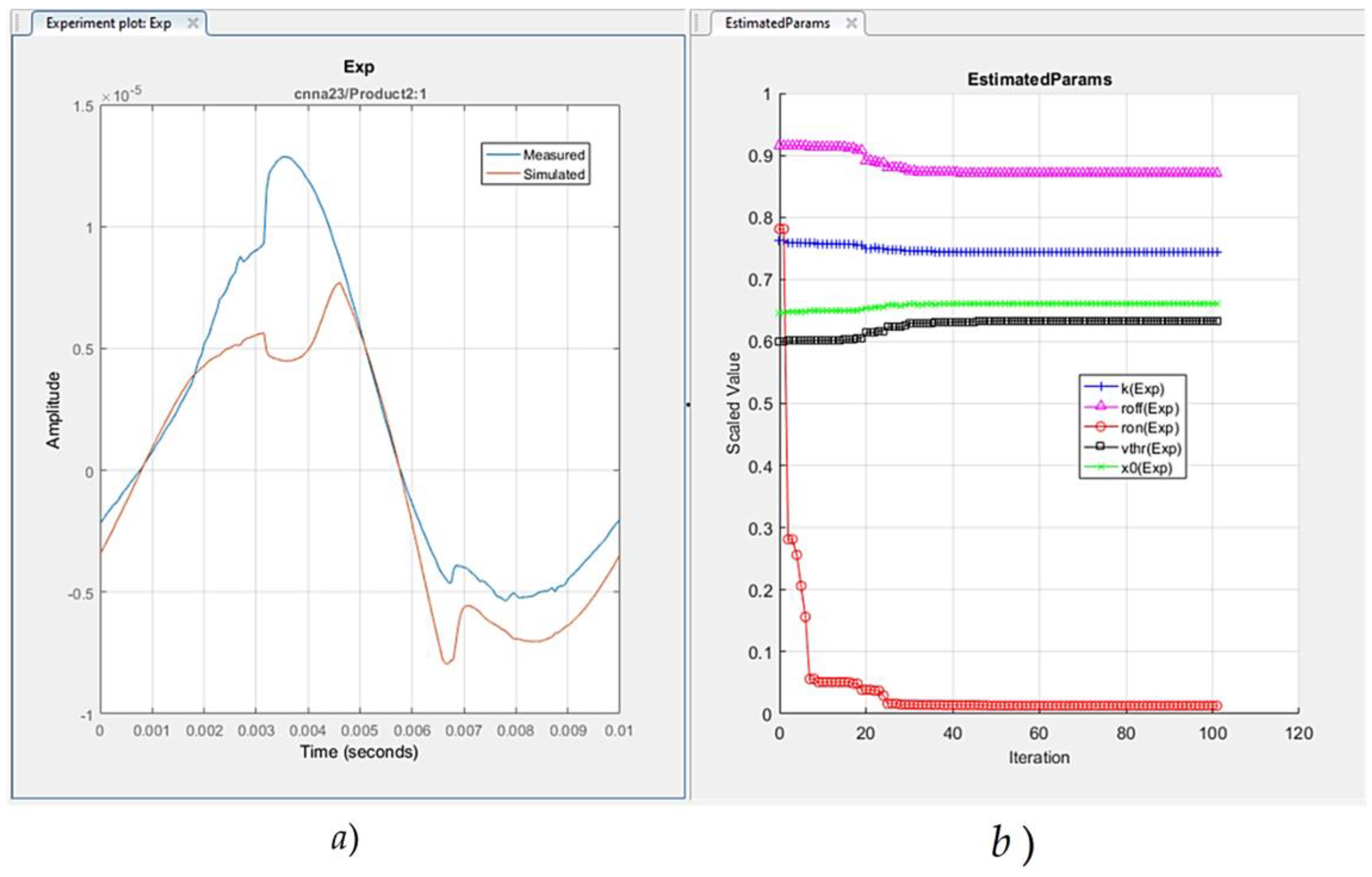
Figure 2.
a) Time diagrams of the experimental and the simulated current after the parameter estimation process, and the state variable of the modified memristor model A14mod; b) Experimental and simulated current-voltage relationships after the parameter estimation process.
Figure 2.
a) Time diagrams of the experimental and the simulated current after the parameter estimation process, and the state variable of the modified memristor model A14mod; b) Experimental and simulated current-voltage relationships after the parameter estimation process.
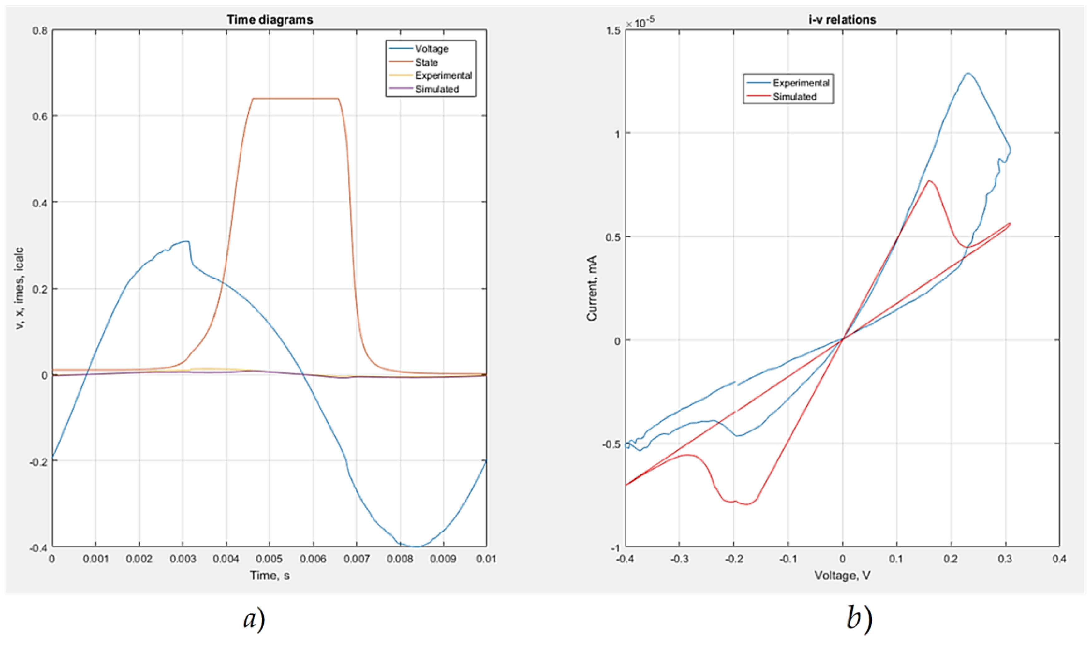
Figure 3.
a) A principal schematic of a memristor model A14mod, included in a simple electronic circuit for analysis at sinusoidal mode, supplied by a voltage source with an amplitude of 1.1 V and different frequencies; b) Current-voltage relation of the model A14mod at 100 kHz; c) i-v characteristic of model A14mod at 1 MHz; d) current-voltage characteristic of the model, obtained at 10 MHz.
Figure 3.
a) A principal schematic of a memristor model A14mod, included in a simple electronic circuit for analysis at sinusoidal mode, supplied by a voltage source with an amplitude of 1.1 V and different frequencies; b) Current-voltage relation of the model A14mod at 100 kHz; c) i-v characteristic of model A14mod at 1 MHz; d) current-voltage characteristic of the model, obtained at 10 MHz.
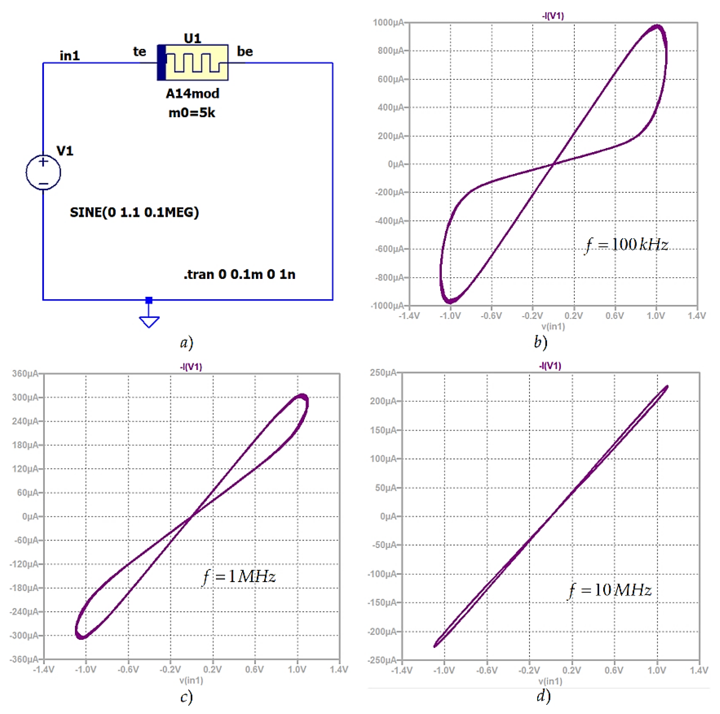
Figure 4.
Memristance adjustment by positive voltage pulses; a) A simple electronic circuit with a memristor and a pulse voltage source; b) time diagrams of the pulse voltage signal with amplitude of 1.1 V and a frequency of 500 MHz, and pulse duration of 1 ns; c) time diagram of the memristance, corresponding to the applied pulses.
Figure 4.
Memristance adjustment by positive voltage pulses; a) A simple electronic circuit with a memristor and a pulse voltage source; b) time diagrams of the pulse voltage signal with amplitude of 1.1 V and a frequency of 500 MHz, and pulse duration of 1 ns; c) time diagram of the memristance, corresponding to the applied pulses.
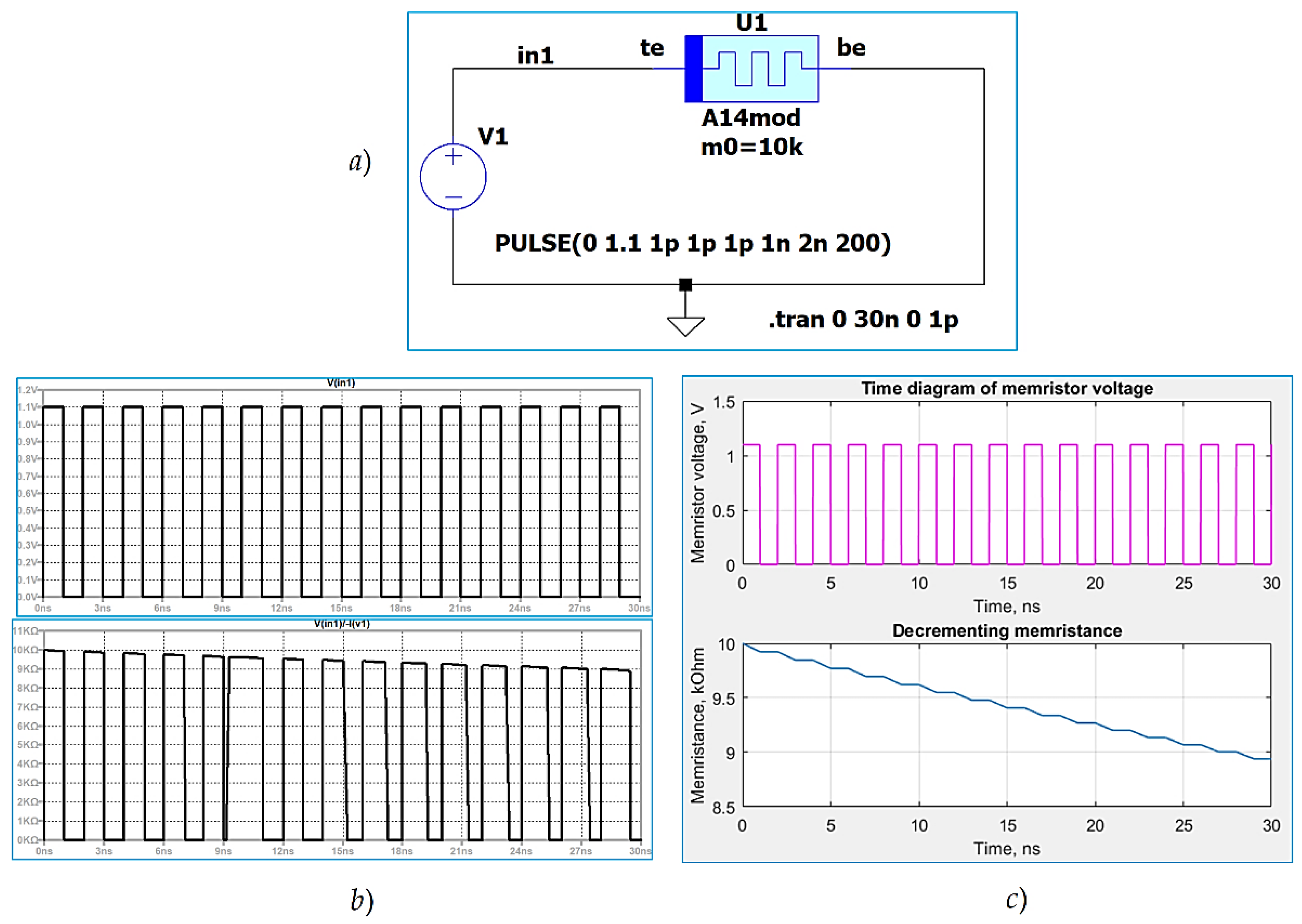
Figure 5.
Memristance adjustment by negative voltage pulses; a) time diagram of the pulse voltage signal with a level of -1.1 V and a frequency of 500 MHz, and pulse duration of 1 ns; b) time diagram of the memristance, corresponding to the applied voltage pulses.
Figure 5.
Memristance adjustment by negative voltage pulses; a) time diagram of the pulse voltage signal with a level of -1.1 V and a frequency of 500 MHz, and pulse duration of 1 ns; b) time diagram of the memristance, corresponding to the applied voltage pulses.
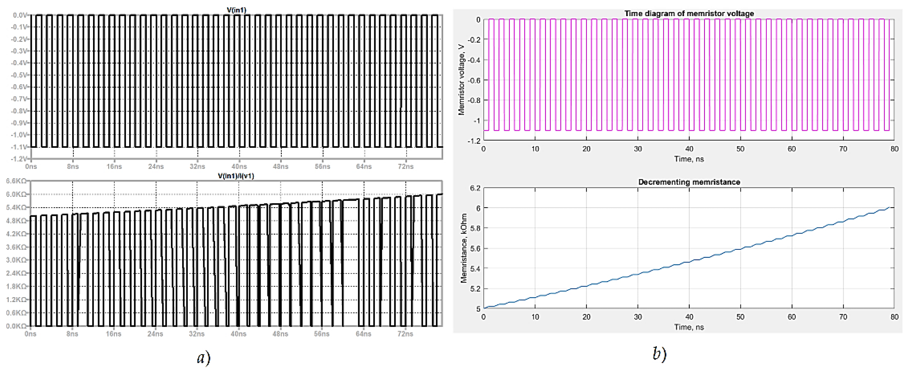
Figure 6.
a) A logarithmic-sigmoidal transfer function, realized by a metal-oxide memristor and two MOS transistors, connected in anti-parallel; b) A transfer function, realized by a voltage-controlled voltage source.
Figure 6.
a) A logarithmic-sigmoidal transfer function, realized by a metal-oxide memristor and two MOS transistors, connected in anti-parallel; b) A transfer function, realized by a voltage-controlled voltage source.
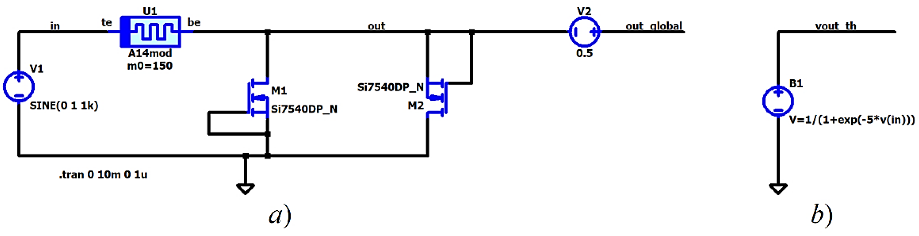
Figure 7.
A comparison of the suggested transfer function, realized by MOS transistors and a memristor – vout_tf_MOS and the theoretical output signal, realized by a voltage-controlled source vout_th = 1/(1+exp(-5*vin)).
Figure 7.
A comparison of the suggested transfer function, realized by MOS transistors and a memristor – vout_tf_MOS and the theoretical output signal, realized by a voltage-controlled source vout_th = 1/(1+exp(-5*vin)).
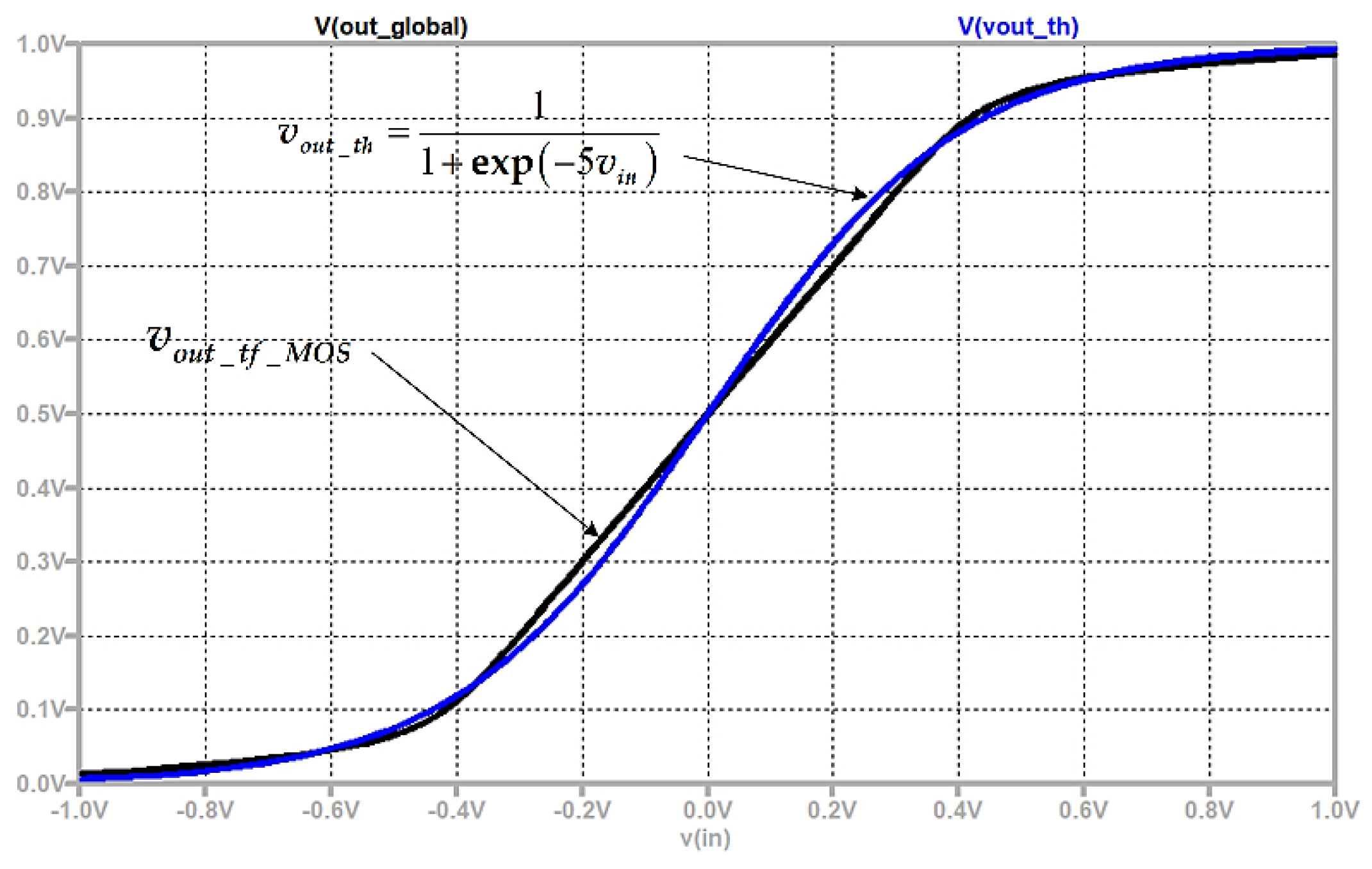
Figure 8.
A block diagram of artificial neuron with memristor-based synapses.
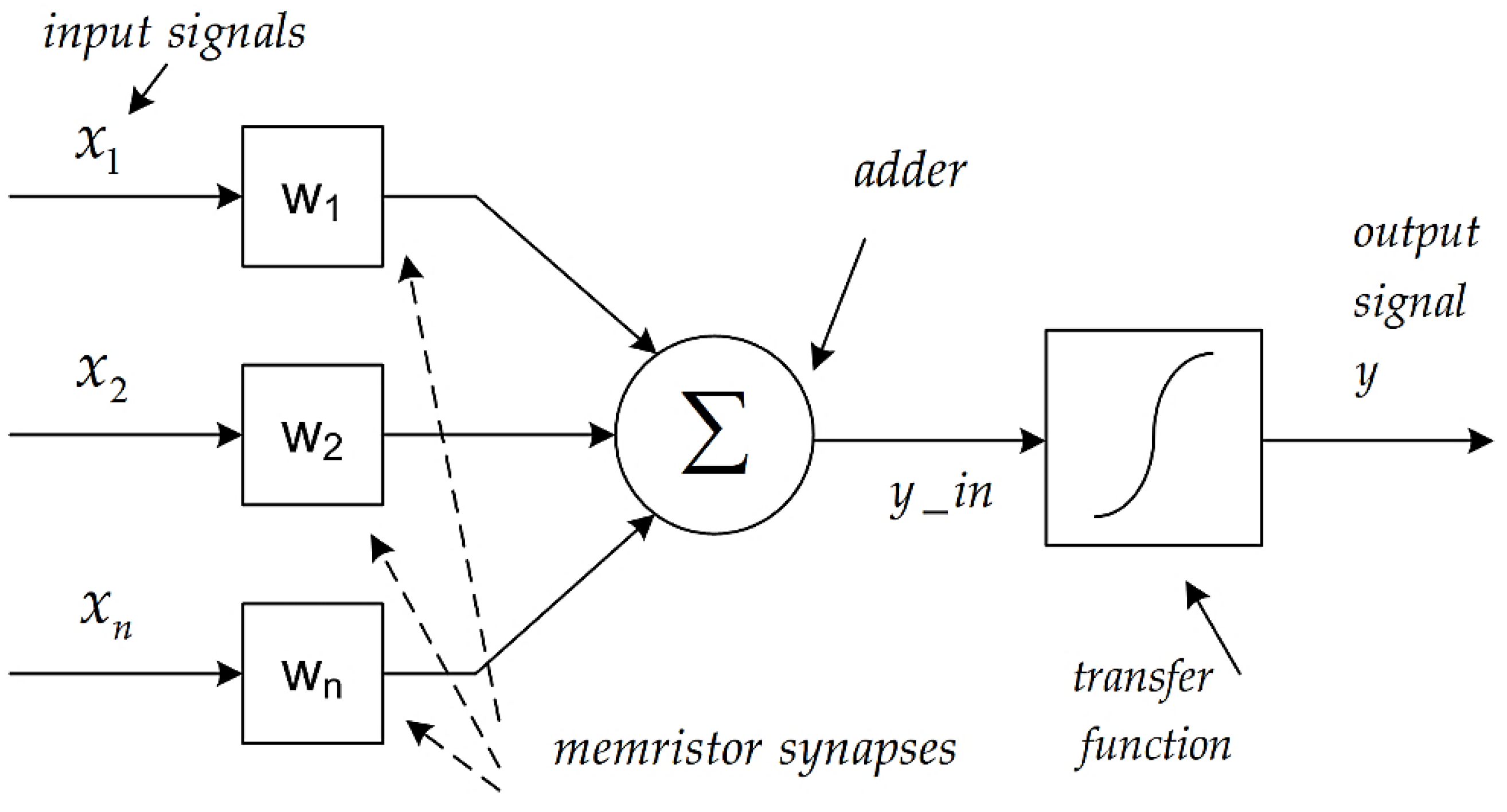
Figure 9.
A principal schematic of metal-oxide memristor-based neuron with negative and positive synaptic weights.
Figure 9.
A principal schematic of metal-oxide memristor-based neuron with negative and positive synaptic weights.
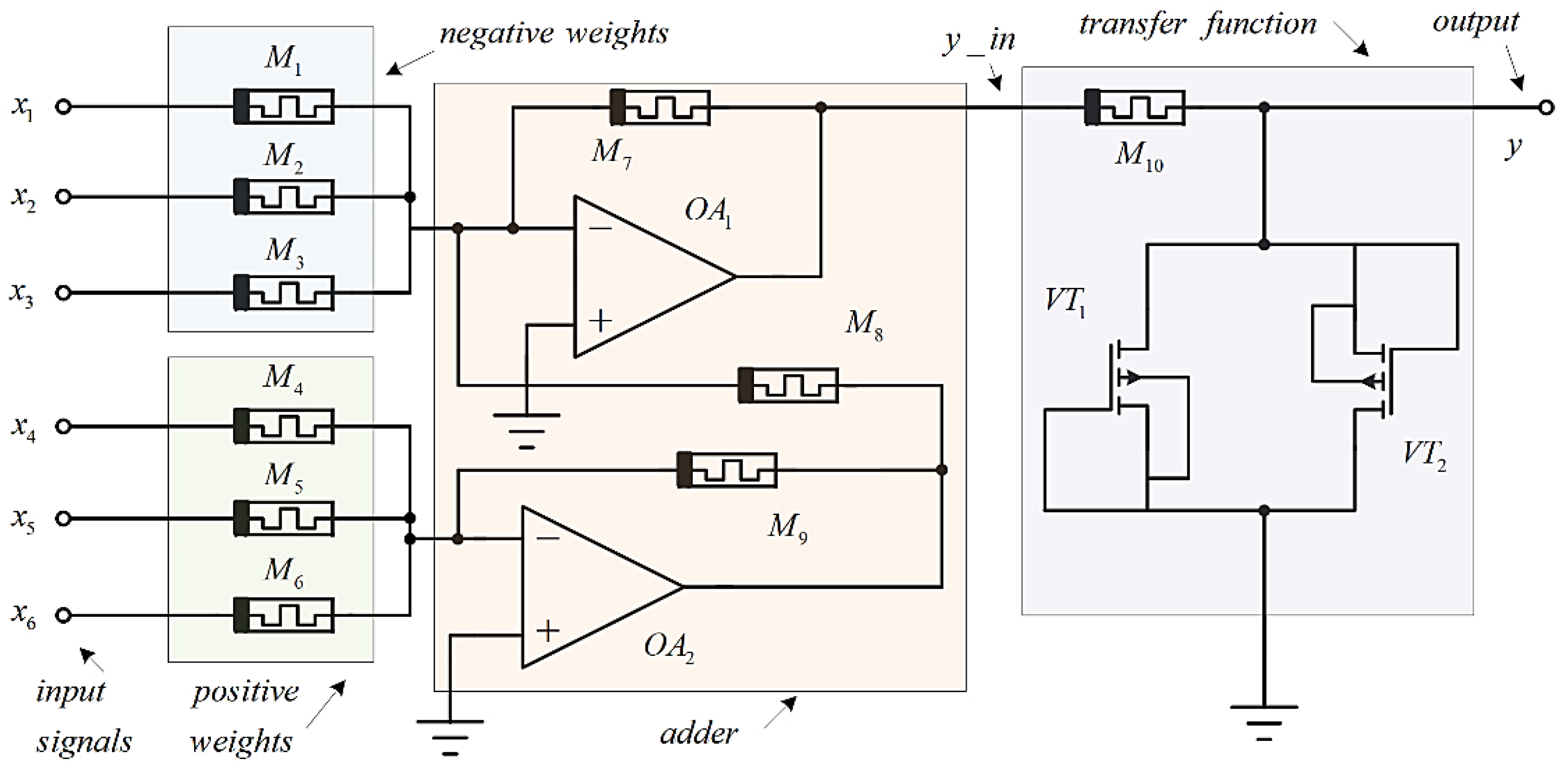
Figure 10.
LTSPICE realization of a model of artificial neuron with memristor synapses and op-amps, included in the adder.
Figure 10.
LTSPICE realization of a model of artificial neuron with memristor synapses and op-amps, included in the adder.
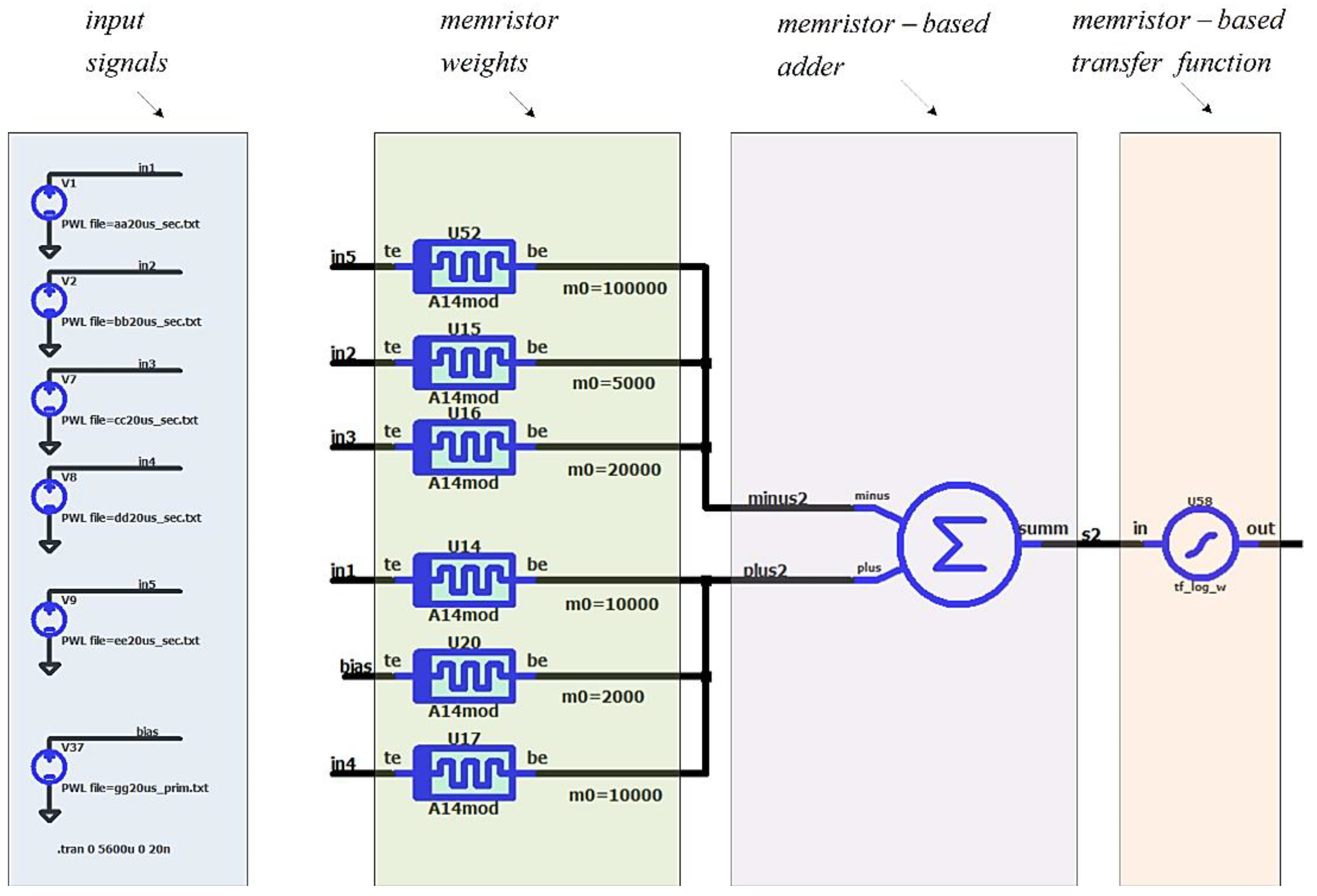
Figure 11.
A realization of the considered memristor-based adder in LTSPICE.
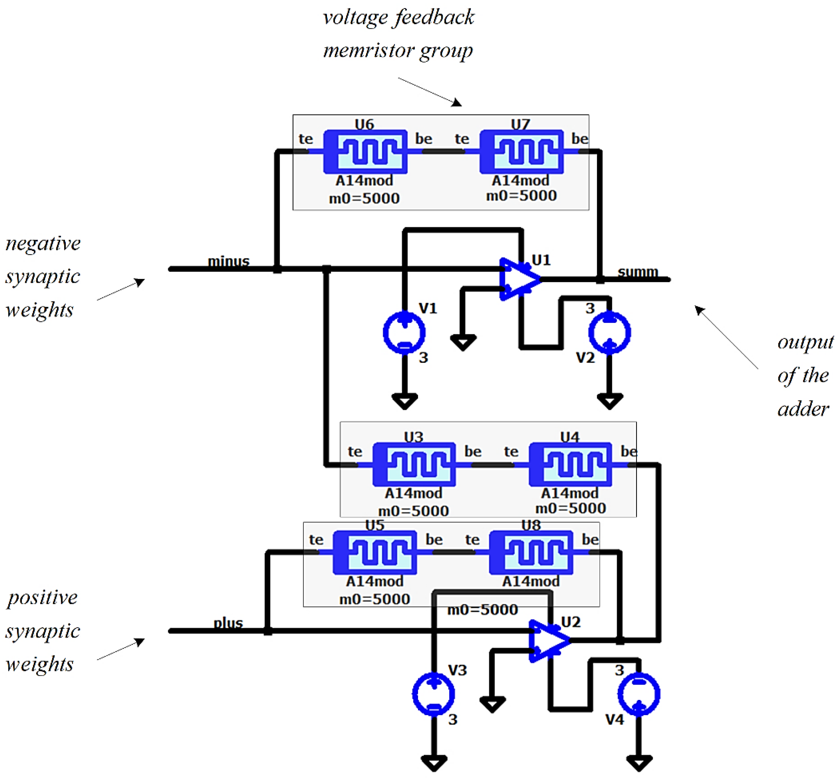
Figure 12.
A voltage divider with memristor, connected to a buffer amplifier in LTSPICE environment.
Figure 12.
A voltage divider with memristor, connected to a buffer amplifier in LTSPICE environment.
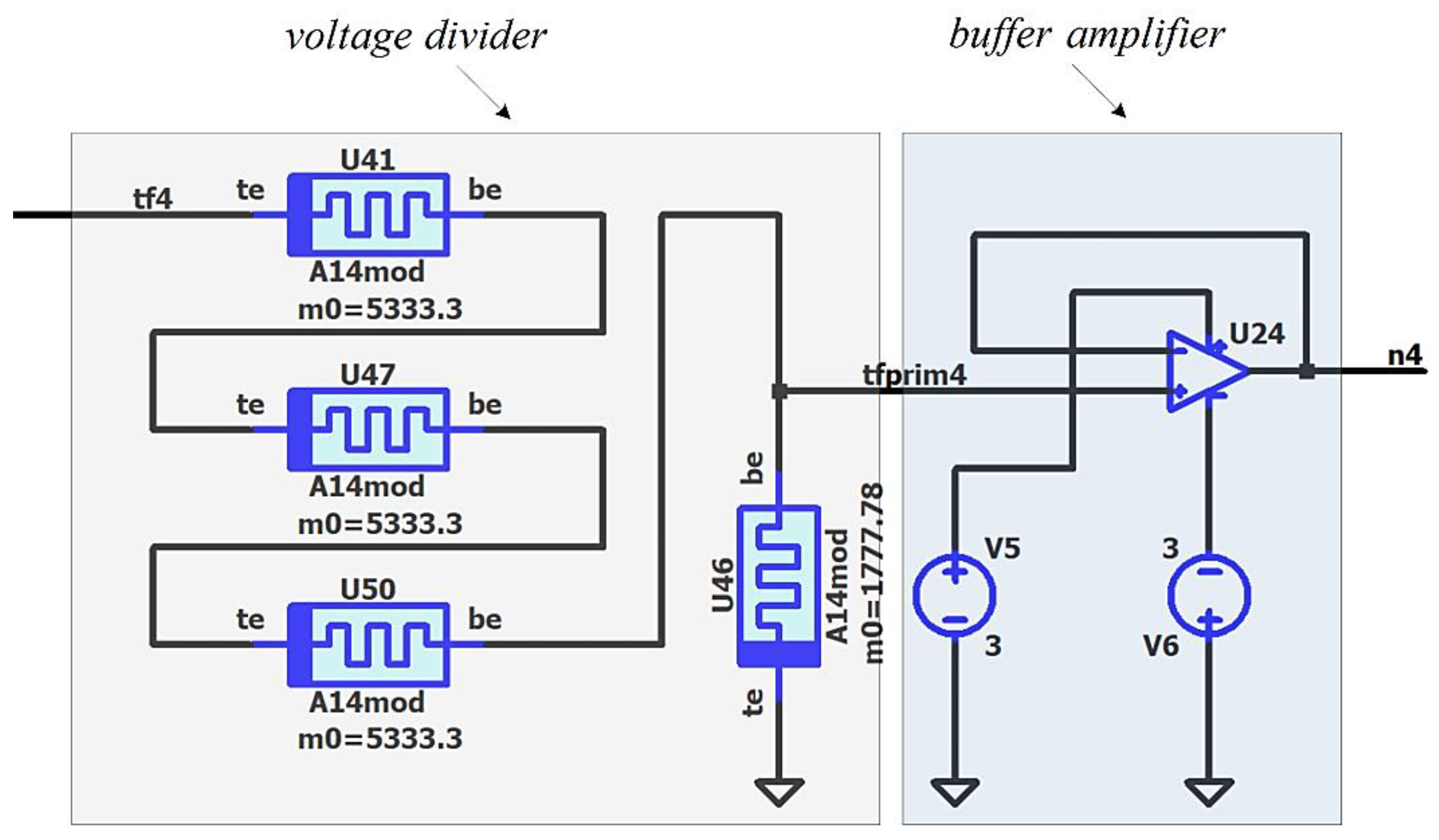
Figure 13.
Block diagram of the considered memristor-based neural network, containing five input nodes, four neurons in the hidden layer and two neurons in the output layer.
Figure 13.
Block diagram of the considered memristor-based neural network, containing five input nodes, four neurons in the hidden layer and two neurons in the output layer.
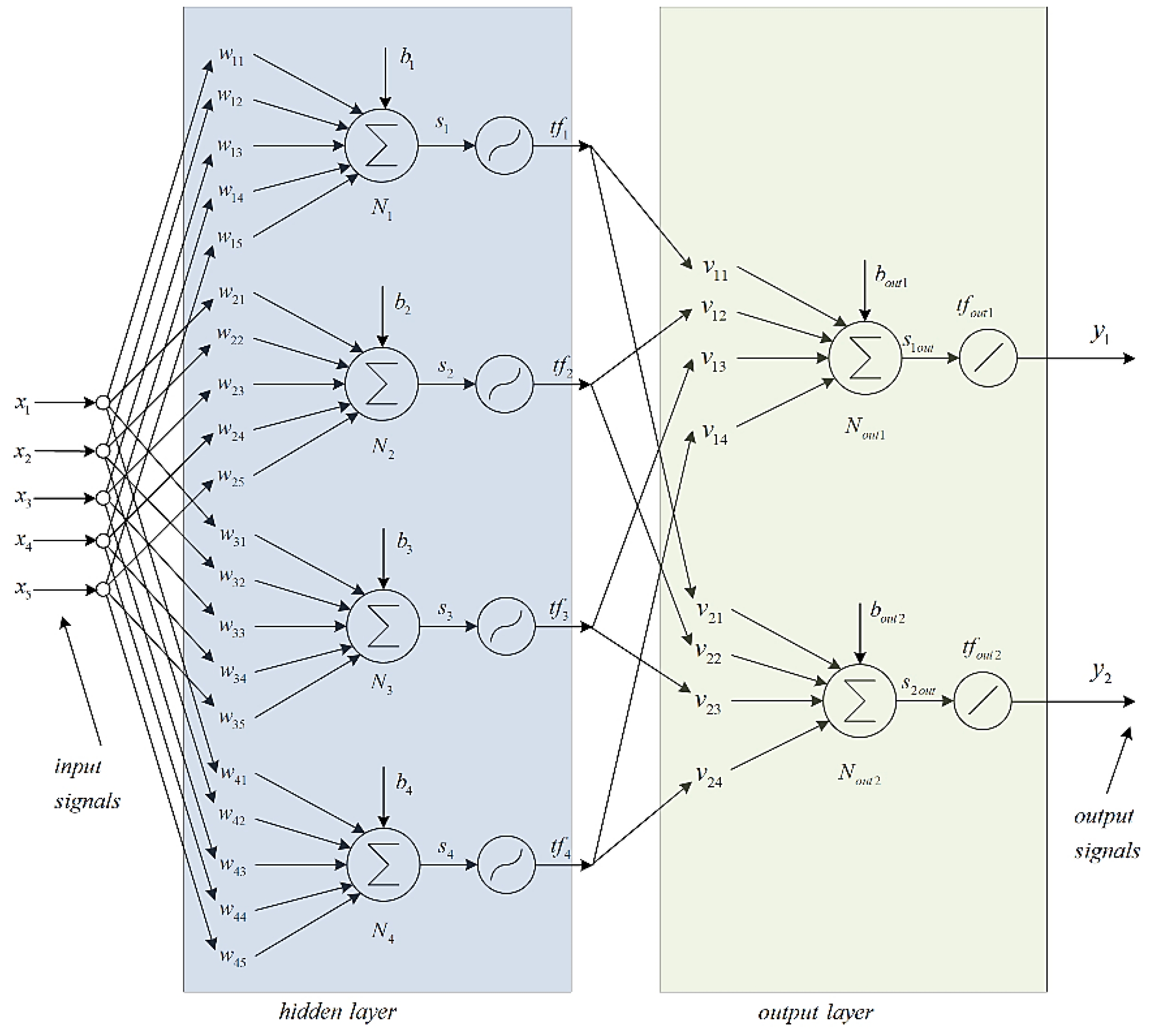
Figure 14.
Principal schematic of the considered memristor-based NN.
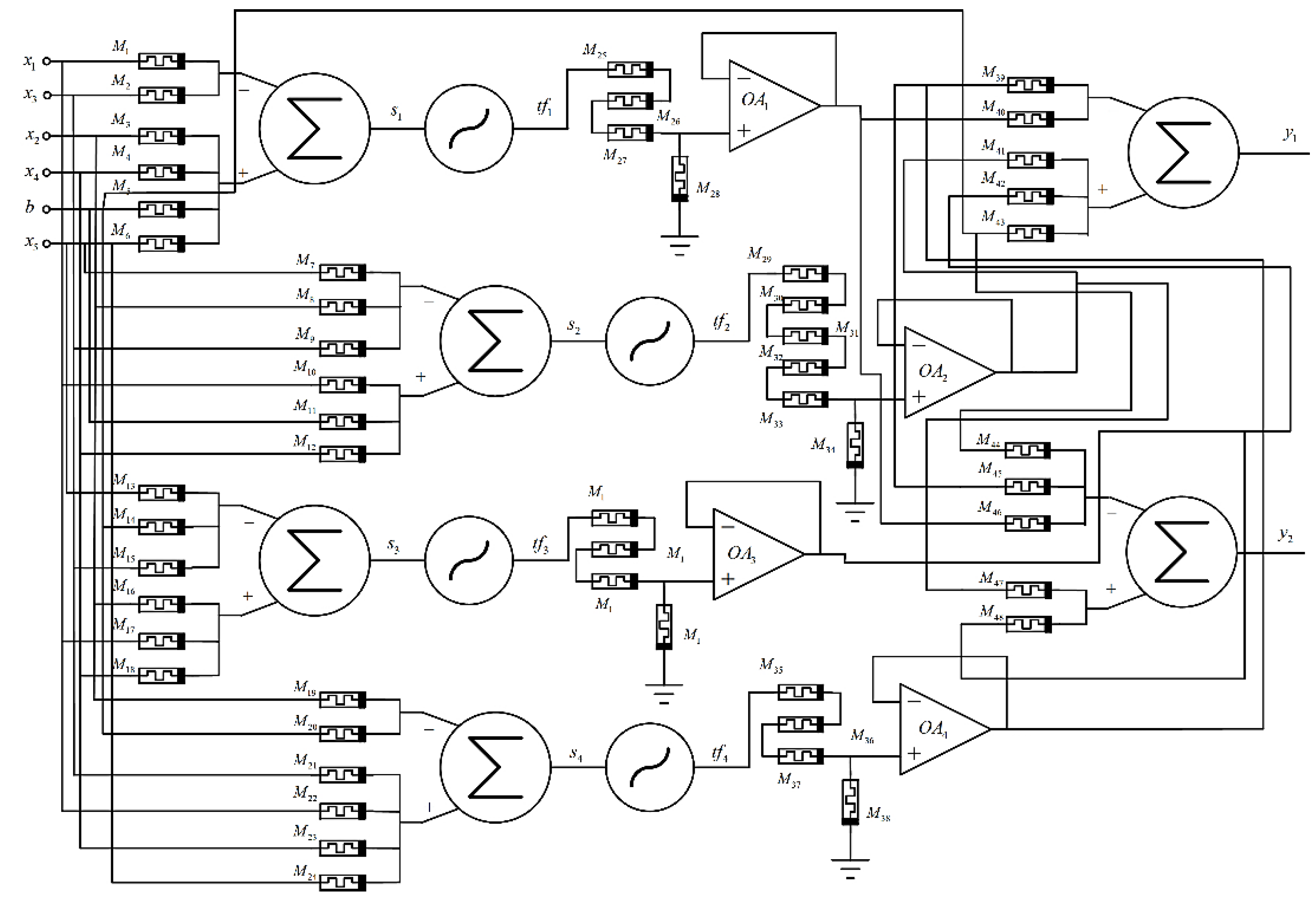
Figure 15.
A realization of the considered memristor-based neural network in electronic simulator – LTSPICE, with five input signals – from in1 to in5, four neurons in the hidden layer and two neurons in the output layer, with memristor-based synapses and MOS-transistor based logarithmic-sigmoidal transfer function.
Figure 15.
A realization of the considered memristor-based neural network in electronic simulator – LTSPICE, with five input signals – from in1 to in5, four neurons in the hidden layer and two neurons in the output layer, with memristor-based synapses and MOS-transistor based logarithmic-sigmoidal transfer function.
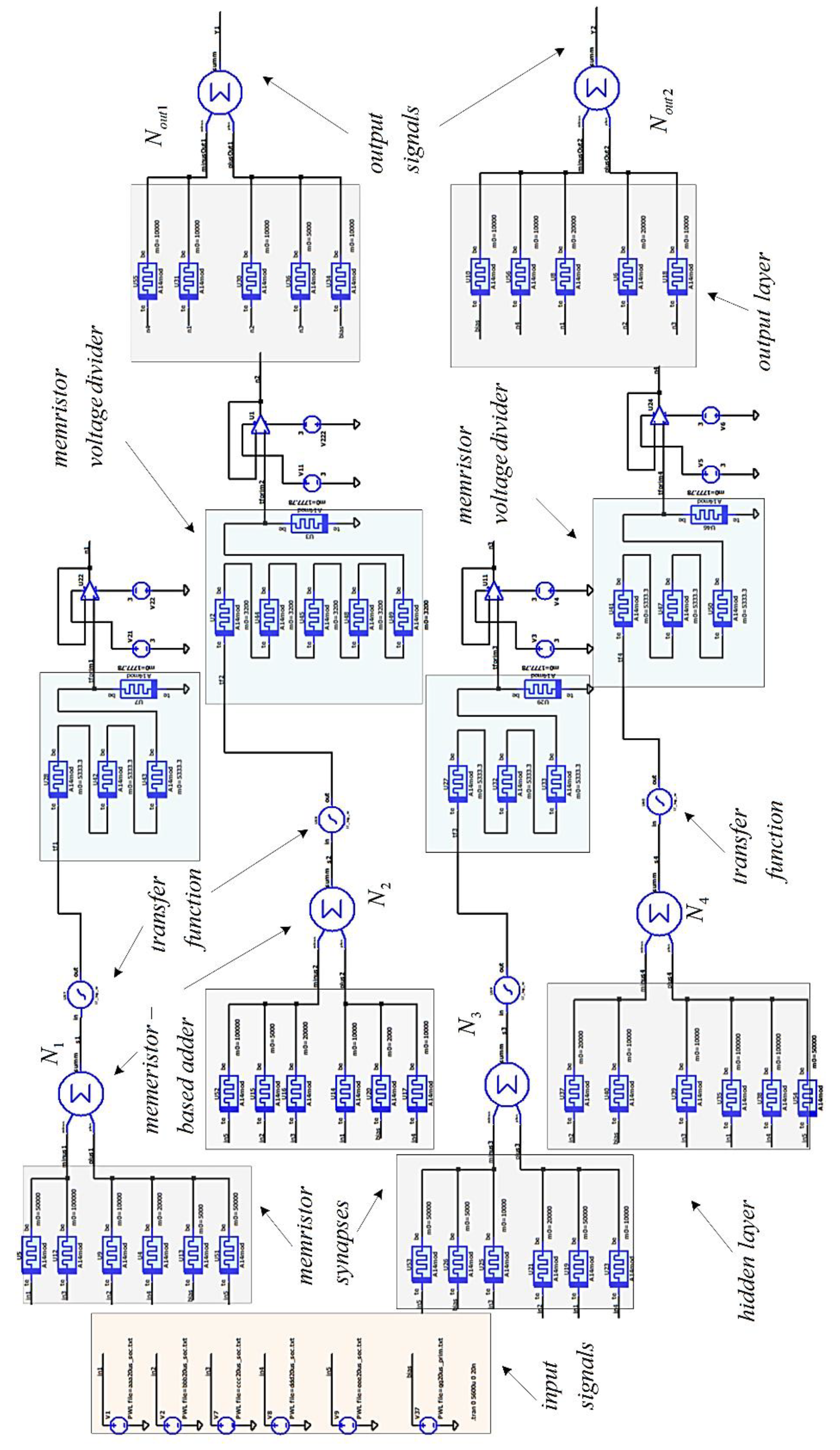
Figure 16.
Analysis of the considered memristor-based neural network in LTSPICE environment; a) Time diagrams of the input signals v1 – v5 and the bias signal vbias; b) graphs of the signals after the adders in the hidden layer - vs1, vs2, vs3 and vs4; c) time diagrams of the signals after the transfer functions in the hidden layer – vtf1, vtf2, vtf3 and vtf4; d) time diagrams of the output signals of the neural network – vy1 and vy2.
Figure 16.
Analysis of the considered memristor-based neural network in LTSPICE environment; a) Time diagrams of the input signals v1 – v5 and the bias signal vbias; b) graphs of the signals after the adders in the hidden layer - vs1, vs2, vs3 and vs4; c) time diagrams of the signals after the transfer functions in the hidden layer – vtf1, vtf2, vtf3 and vtf4; d) time diagrams of the output signals of the neural network – vy1 and vy2.
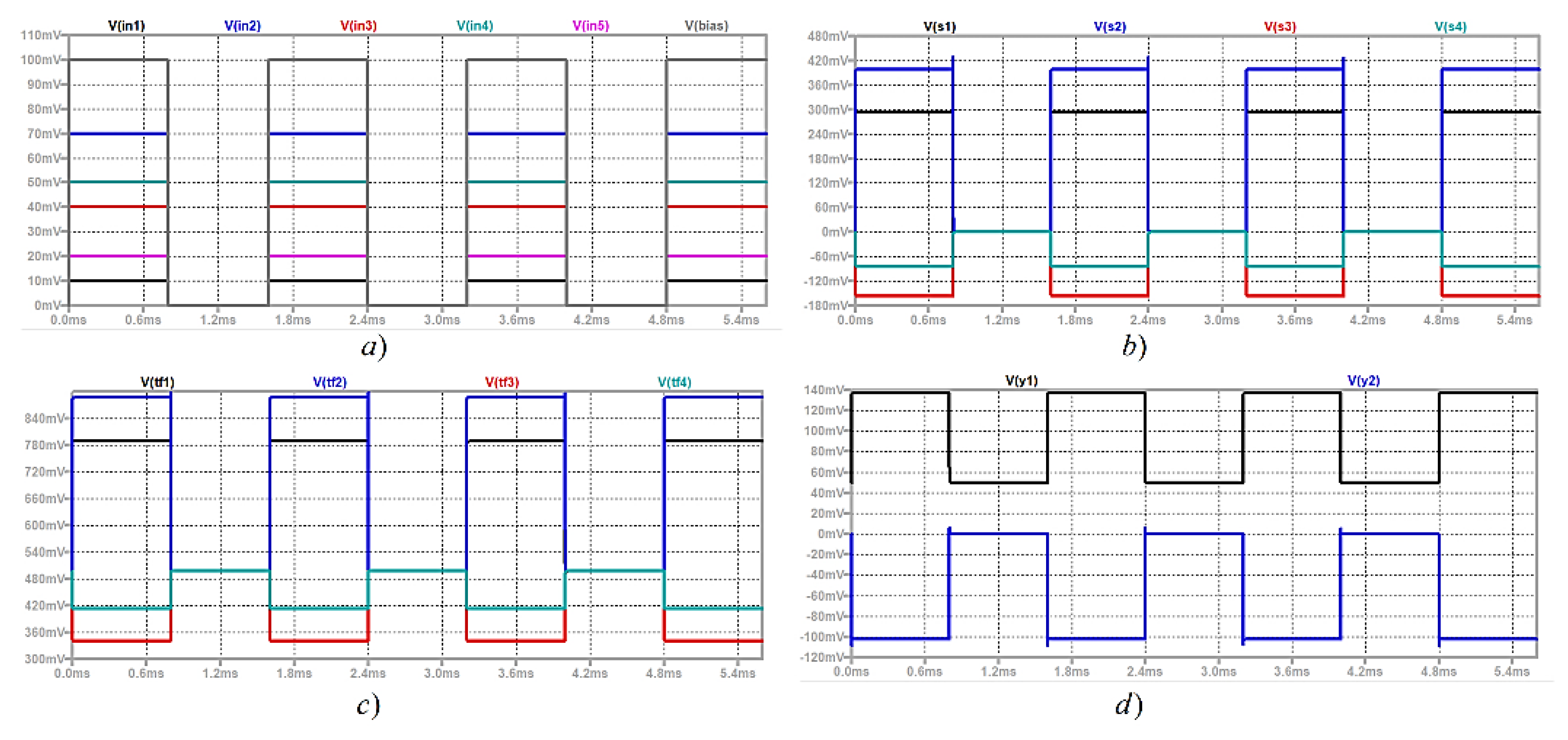
Figure 17.
Simulink diagram of the analyzed memristor-based neural network.
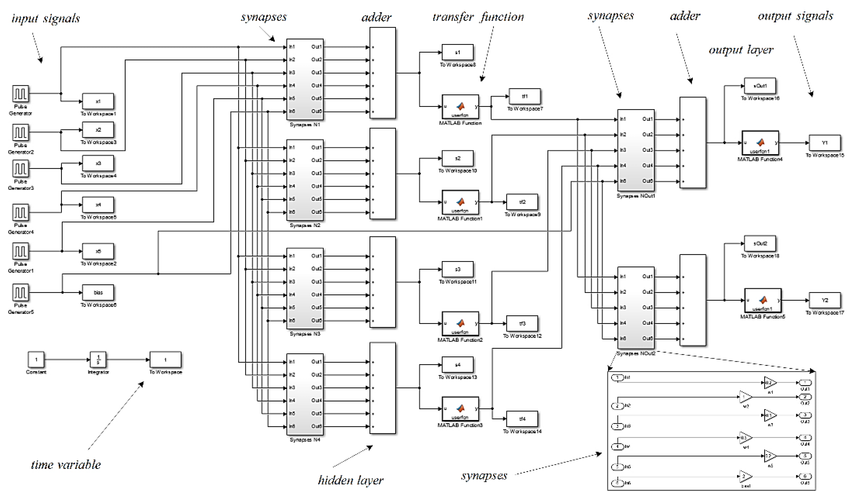
Figure 18.
Time diagrams, corresponding to the neural network presented in Figure 15; a) time diagrams for the input signals; b) for the hidden layer – the output signals of the adders and of the transfer functions; c) time diagrams for the output layer – the output signals of the adders and these of the output transfer functions.
Figure 18.
Time diagrams, corresponding to the neural network presented in Figure 15; a) time diagrams for the input signals; b) for the hidden layer – the output signals of the adders and of the transfer functions; c) time diagrams for the output layer – the output signals of the adders and these of the output transfer functions.
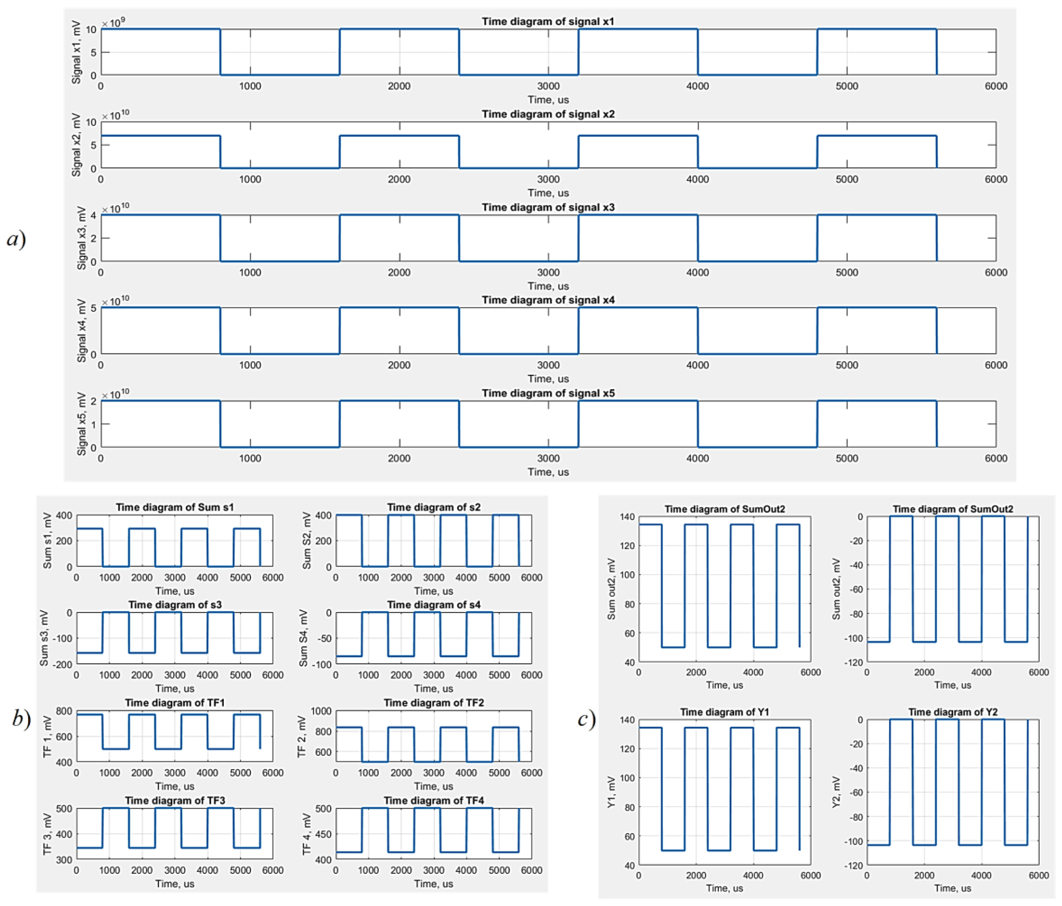

Table 1.
A short comparison of the considered metal-oxide memristor models – Joglekar, Biolek, Lehtonen-Laiho, and the applied modified memristor model A14mod [35].
Table 1.
A short comparison of the considered metal-oxide memristor models – Joglekar, Biolek, Lehtonen-Laiho, and the applied modified memristor model A14mod [35].
| Model | Joglekar [22] | Biolek [23] | Lehtonen-Laiho [21] | A14mod [35] |
|---|---|---|---|---|
| Switching properties | middle | satisfactory | good | good |
| Frequency | low | low, middle | high | high |
| RMS error | 17.6 | 16.3 | 3.4 | 14.2 |
| Complexity | low | middle | high | low |
| Simulation time, ms | 15.4 | 16.7 | 18.3 | 17.5 |
Table 2.
Comparison of the applied memristor models, according to simulation time.
| Case | Models | Joglekar [22] | Biolek [23] | Lehtonen-Laiho [21] | A14mod [35] |
|---|---|---|---|---|---|
| Decreasing memristance | Simulation time, ms | 28.2 | 30.8 | 35.8 | 28.3 |
| Increasing memristance | Simulation time, ms | 28.5 | 31.1 | 37.8 | 24.3 |
Table 3.
Input and bias signals for the memristor-based neural network, to be realized in LTSPICE.
| Input signals, mV | Bias signal, mV | ||||
|---|---|---|---|---|---|
| vin1 | vin2 | vin3 | vin4 | vin5 | vbias |
| 10 | 70 | 40 | 50 | 20 | 100 |
Table 4.
Synaptic weights for the hidden layer of the considered memristor NN in LTSPICE.
| Synaptic weights for the hidden layer | ||||||
| Neuron | w1 | w2 | w3 | w4 | w5 | wbias |
| N1 | -0.2 | 1 | -0.1 | 0.5 | 0.2 | 0.2 |
| N2 | 1 | -2 | -0.5 | 1 | -0.1 | 0.5 |
| N3 | 0.2 | 0.5 | -1 | 1 | -0.2 | -0.2 |
| N4 | 0.1 | -0.5 | 1 | 0.1 | 0.2 | -0.1 |
Table 5.
Memristances for the synapses in the hidden layer of the considered NN in LTSPICE.
| Input memristances, kOhms | ||||||
| Neuron | M1 | M2 | M3 | M4 | M5 | Mbias |
| N1 | -50 | 10 | -100 | 20 | 50 | 5 |
| N2 | 10 | -5 | -20 | 10 | -100 | 2 |
| N3 | 50 | 20 | -10 | 10 | -50 | -5 |
| N4 | 100 | -20 | 10 | 100 | 50 | -10 |
Table 6.
Synaptic weights for the output layer of the considered NN in LTSPICE.
| Synaptic weights for the output layer | |||||
| Neuron | M1out | M2out | M3out | M4out | Mbiasout |
| N1out | -0,1 | 0,1 | 0,2 | -0,1 | -1 |
| N2out | -0,05 | 0,05 | 0,1 | -0,1 | -0,5 |
Table 7.
Memristances for the output layer of the considered NN in LTSPICE.
| Output layer memristances, kOhms | ||||||
| Neuron | M1 | M2 | M3 | M4 | M5 | Mbias |
| N1 | -10 | 10 | 5 | -10 | -10 | 10 |
| N2 | -20 | 20 | 10 | -10 | -20 | -10 |
Table 8.
Comparison between the results, obtained after the analyses of the memristor-based neural net.
Table 8.
Comparison between the results, obtained after the analyses of the memristor-based neural net.
| Signals | S1 | S2 | S3 | S4 | tf1 | tf2 | tf3 | tf4 | Y1 | Y2 |
| mV | mV | mV | mV | mV | mV | mV | mV | mV | mV | |
| Simulink | 293 | 398 | -157 | -85 | 769 | 836 | 344 | 414 | 134 | -104 |
| LTSPICE | 293 | 398 | -157 | -85 | 789 | 887 | 342 | 413 | 137 | -102 |
| MATLAB | 293 | 398 | -157 | -85 | 769 | 836 | 344 | 414 | 134 | -105 |
Disclaimer/Publisher’s Note: The statements, opinions and data contained in all publications are solely those of the individual author(s) and contributor(s) and not of MDPI and/or the editor(s). MDPI and/or the editor(s) disclaim responsibility for any injury to people or property resulting from any ideas, methods, instructions or products referred to in the content. |
© 2024 by the authors. Licensee MDPI, Basel, Switzerland. This article is an open access article distributed under the terms and conditions of the Creative Commons Attribution (CC BY) license (http://creativecommons.org/licenses/by/4.0/).
Copyright: This open access article is published under a Creative Commons CC BY 4.0 license, which permit the free download, distribution, and reuse, provided that the author and preprint are cited in any reuse.