Submitted:
14 January 2024
Posted:
15 January 2024
You are already at the latest version
Abstract
Reconstructing a 3D model of a scene from a set of multiple views poses a significant challenge in the field of computer vision. The advent of NeRF has marked a major breakthrough in this domain. However, there is a need to extend the capabilities of the NeRF model to enable editing tasks such as relighting and deformation, as well as to enhance its training efficiency. Neural reflectance fields introduce the concept of the reflectance equation into the NeRF framework to achieve relighting of the NeRF model. We leverage the TensoRF approach, which incorporates tensor decomposition and employs multiple tensors to store features, to expedite the training process of the NeRF model. Our novel method, called StensorR, combines the reflectance equation and tensor decomposition within the radiation field model framework. Differing from previous approaches, we employ a single tensor to store scene features and render the surface color of our scene using a simplified reflectance equation. This approach accelerates model convergence and enables relighting of the NeRF model. Experimental results demonstrate that our method achieves a 50% faster convergence rate compared to existing relighting radiation field models, while successfully enabling relighting and improving the quality of synthesized images from new viewpoints.
Keywords:
computer vision
; 3D Reconstructing
; NeRF
; relighting
; the reflectance equation
; tensor representation
1. Introduction
The reconstruction from 2D image to 3D representation is an important research branch in the field of computer vision and graphics. Radiance fields [1,2,3,4] represent a significant breakthrough in this research direction. It establishes a radiation field through a series of images of some target objects or scenes taken by the synchronous camera; and then uses MLP, voxel grid [5,6,7,8,9] or muti-tensor [10,11] as the representation of the target scene object or scene, which is to convert the rigid body into a mutually occlusive light source (i.e., particles that emit light and absorb light) filled in the space, so as to realize the optimization of the whole space and greatly reduce the difficulty of solving the reconstruction problem. However, the geometry, material, lighting, and other geometric attributes of objects are coupled into density and appearance by the optimization operation of the radiance fields model. Although this coupling operation can achieve excellent rendering results with few resources and costs, it greatly sacrifices flexibility. A typical example is the inability to edit and relight the radiance fields model.
As for relighting [12,13], a widely accepted and mature approach is to incorporate the Reflectance Equation [14], which is the core function of Physically Based Rendering, which has the best simulation effect in the field of computer vision and graphics. This model is not only based on the microface surface model; but also considers the conservation of energy. It also applies the bidirectional reflectance distribution function (BRDF) based on physics, so it has an exceptional effect. The reflectivity equation is mainly composed of two parts, the radiance equation and BRDF [15]. The radiance equation is described as the total energy of the light source on the unit area and the unit solid angle [16]. This is a differentiable quantity. By Riemann summation with the BRDF function at the corresponding position, we can approximate the sum of reflected light of the geometric surface under a specific light source, and use it to represent the color value of the geometric mode. When the reflectance equation is applied to express the color value of the radiance fields model, and then the model can be re-illuminated by changing the light source or changing the properties of geometric surface [17,18,19].
In this paper, we propose a novel relighting solution for implicit scene reconstruction——a tensorial able relighting radiance field for single-tensor scene representation, simple training data requirements, high-quality new perspective generation results, and efficient relighting.
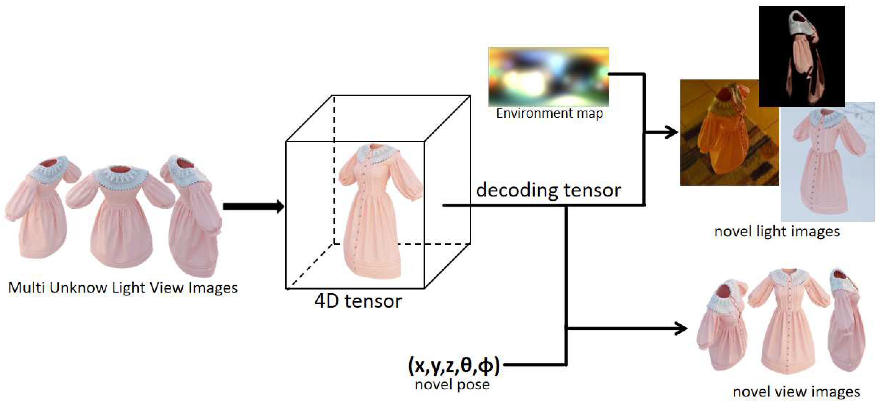
Figure 1.
Our method trains a 4D tensor field using multi-view captured images of a scene with unknown illumination. This tensor field enables the generation of high-quality scene images under new illuminations and new viewing angles, based on input new pose and illumination.
Figure 1.
Our method trains a 4D tensor field using multi-view captured images of a scene with unknown illumination. This tensor field enables the generation of high-quality scene images under new illuminations and new viewing angles, based on input new pose and illumination.
Our method represents the scene using a 4D tensor, which undergoes decomposition into several low-rank tensor components. Each feature grid comprises one-dimensional density values and multi-dimensional appearance features. These appearance features are simultaneously fed into the color network, normal network, and BRDF decoder. Consequently, the color value, normal value, and BRDF value of each point are obtained. To render the surface pixel color, we employ spherical Gaussians to simulate the incident light field, incorporating the normal value and BRDF value. By combining the scene density value, the calculated color value, and volume rendering techniques, we optimize the scene and determine the positions of the surface points. In contrast to previous radiation field methods that rely on multiple voxel meshes or tensors [5,6,7,8,9,10,11], our approach utilizes a single 4D tensor to represent the scene. We leverage tensor decomposition [10,11,20] techniques to expedite the optimization process for the scene. Unlike previous methods for relighting the radiation field by combined reflectance equation [11,21,22,23,24,25,26,27], our approach incorporates a network that directly estimates the amount of light reflected from a specific point. This estimation aligns conceptually with the output of BRDF, and therefore, we refer to it as the BRDF value. By combining this value with the secondary reflected light field, we approximate the integral of the reflected light on the hemispherical surface of the scene surface point.
In summary, our contributions are as follows:
- We propose a tensorial able relighting radiance field for single-tensor scene representation.
- We achieve visual quality comparable to the previous state-of-the-art model at a rendering and relighting speed is about 1.5× faster.
- Our model training does not rely on complex geometric surface properties.
2. Releate Work
2.1. Representations for Novel View Synthesis
Neural scene representations have emerged as a promising and innovative alternative to traditional representations such as meshes, volumes, and point clouds, revolutionizing the generation and modeling of 3D content. Image synthesis from novel viewpoints, based on a series of observed pictures of a scene, has been a longstanding task that has garnered significant research attention, and the neural scene representation has shown excellent performance in this task. [1,2,3,4] In the original NeRF model, crucial information such as spatial coordinates, color, and density is encapsulated within an MLP, which resulted in the MLP’s deep architecture and high-dimensional characteristics. As a consequence, the training process exhibited a slow convergence rate. In recent research efforts, several improved approaches have emerged. Some methods utilize voxels instead of MLP to represent the spatial coordinates of 3D points, storing color and density features within the voxel structure [5,6,7,8,9]. By incorporating activated density voxel grids, these methods achieve rapid convergence rates. Other approaches employ multi-scale hashing to encode input coordinates into feature vectors and leverage simple MLP architectures for high-quality, fast rendering [28]. Additionally, some methods leverage a low-resolution voxel grid combined with high-resolution 2D grids on three projection planes. By interpolating features, they achieve high-quality, high-speed rendering while minimizing memory consumption. Furthermore, tensor-factorized techniques are employed to decompose 4D tensors into compact, low-rank tensors, enabling high-quality and rapid reconstruction [10,11]. Our tensorial relighting field uses the TensoRF [10] model as a geometric before achieve efficient and realistic 3D content relighting.
2.2. NeRF with Reflectance Equation
NRF [17] introduced the reflection equation into Nerf for the first time. NRF does not assume objects as luminescent particles but particles with reflective properties, and external light sources provide illumination. NeRV [21] further optimized the NRF, breaking away from the strong assumption of flashing lights and modeling-optimized ambient lighting. It also considered one-bounce indirect illumination and introduced Visibility to represent the proportion of energy particles that can reflect light to model indirect lighting, further improving the flexibility of the reflectivity equation. In the NeRFactor [25], a two-stage strategy was directly adopted to completely decouple geometric modeling and color rendering in NeRF. First, use NeRF [1] to recover the target object’s geometry or scene, then restore BRDF [15] and lighting [29,30,31,32]. In the processing of BRDF, real situation collected BRDF information (albedo, normal, metallicity, roughness) was introduced prior to simplifying the modeling of BRDF. Our lighting field model also follows the two-stage strategy, using TensoRF to restore the scene geometry. Then use a neural network to fit the BRDF and combine it with a lighting estimation model to reconstruct realistic 3D content.
3. Method
Our proposed method utilizes a four-dimensional tensor, employing a set of vectors and matrices (VM decomposition), to model the scene [10,11,20]. The first three dimensions correspond to location information, while the fourth dimension represents the scene vector. Within the vector, the initial element denotes the density value of the scene at that particular location, while the remaining elements characterize appearance features. We employ distinct MLP and BRDF decoders to decode the color value, normal vector, and BRDF value at the corresponding scene location. Scene relighting is achieved by combining the rendering equation with an environment map [27,33].
Specifically, our process begins from the origin and incorporates the camera pose to sample the color value and volume density of points along a ray within the tensor field. Volume rendering is then employed to obtain the pixel color value under the given pose. By comparing the acquired color values with the corresponding pixel values in real images, we can estimate the volume density for each point and then estimate the scene surface. [34] The normal vector and BRDF value are subsequently decoded from the appearance features of surface points. We combine this information with environment maps which fitting by 32 spherical Gaussian and render the scene using a formula similar to the reflectance equation. Throughout the process, we monitor and optimize the rendering results, iteratively refining our 4D tensor.Our approach overview is shown in Figure 2.
3.1. Scene Representation
In practical applications, we have formulated a 4D scene tensor , wherein the initial three dimensions correspond to the three-dimensional coordinates (x, y, z), while the fourth dimension represents the feature vector of the scene at those coordinate points. To expedite the training process of the tensor field, we employ vector-matrix factorization to decompose our 4D tensor field into low-rank tensors [10].
For simplicity, let denote the two axes orthogonal to m (e.g. =YZ), while and represent the vector and matrix factors of their corresponding spatial axes m. represent the characteristic component of their corresponding spatial axes m.
By performing linear interpolation of the scene tensor , we can obtain the scene feature vectors.In a similar manner to the approach employed in TensoRF, we adopt an interpolation strategy for the decomposed tensor factors to mitigate computational and storage expenses associated with the model.The scene feature vector F at point x can be write as:
Where the ijk corresponds to the coordinate value corresponding to the orthogonal axis represented by m and .(for example, m=Y, =XZ, then ijk corresponds to the yxz coordinate value of point x respectively)
The first element of the feature vector represents the volume density value of the point, The volume density at point x can be write as:
Correspondingly, we regard the remaining portion of the feature vector as the appearance feature of the scene.The scene feature vector a at point x can be write as:
Where the L denote the length of feature vector.
Input the appearance feature into multiple distinct networks for decoding color values, normal vectors, and BRDF values. The decoder takes the appearance feature vector a, 3D surface point x, view direction d and optional parameters p (like albedo and roughness) as input, and returns three-channel as output.
Furthermore, we employ two MLP to represent the color decoding function and the geometric surface normal vector function:
The MLP receives the appearance feature vector a, the coordinate of point X and view direction d(only for color function) as inputs, producing the RGB values and a three-channel surface normal as respective outputs.
3.2. Incident Light Field
To accurately relight the radiation field, it is crucial to closely approximate formula 14. Our approach imitate the incident light simulation method of [27], which computes the incident light at surface points within the scene based on three key factors:
- the direct light from the light source in the scene;
- the direct light received by the surface point;
- the indirect light reflected from other surface points [35].
3.2.1. Direct Light
We utilize a set of 32 environment maps parameterized by muti-spherical Gaussian (SGs) to represent global illumination. [36] The spherical Gaussian function and the representation of global illumination i.e. the environment map [33], can be expressed as follows:
The RGB value of each pixel in the environment map is simulated using the aforementioned 32 spherical Gaussian mixture. In this simulation, v represents the light angle, while u, a, and are three trainable parameters. Subsequently, spherical Gaussian mixture is employed to represent the direct light emitted by the light source within the scene.
3.2.2. The Transmittance Function
The transmittance function models the receiving rate of the surface point receiving direct light,
The transmittance function here is similar to that in NeRF [1], but in our method it only calculates the transmittance of the last point sampled along the ray.
3.2.3. Indirect Light
An MLP network is used to fit the indirect light reflected from other surface points directly.
where the MLP takes the appearance feature vector a, 3D surface point x and view direction of surface point d as input, and returns the 3-channel indirect light RGB value as output. Overall, our lighting simulation formula can be written as:
3.3. The Rendering Equation
In the preceding sections, we presented the scene representation employed in our method and discussed the approach for simulating incident light. In the following sections, we will introduce our two rendering equations and subsequently leverage the combined rendering results to optimize our scene tensor. The first rendering equation corresponds to the volume rendering formula employed in NeRF. It involves emitting ray from the origin, o, in the direction, d, and sampling N points along the ray. These sampled points are then employed in the following formula to compute the pixel value.
Where is the discretization calculation method of equ 10.
The second rendering equation integrates the reflectance equation. [11,18] It computes the color value of the surface point , observed from the direction by considering the reflection of all incident light on the hemispherical surface centered at .
In practice, calculating the fraction of a spherical area requires discretizing and summing the aforementioned formula, which can be computationally expensive. Therefore, to approximate the surface integral, we opt to utilize the incident light field discussed in the previous section and incorporate indirect illumination the actual formula can be reformulated as follows:
where denotes the BRDF value decoded by in Equ 5, represents the overall ambient light computed in Equ 8. We supervise the pixel value calculations obtained from the two rendering equations in order to optimize our tensor field.The loss function written as:
Specifically, Equ 15 applies to the surface points within the scene. Prior to a certain number of iterations (before obtaining the scene surface), the value of is set to zero. However, once this threshold is reached, gradually decreases over subsequent iterations.
3.4. The BRDF Decoder
In the preceding sections, we provided a comprehensive description of our model structure and process. In the subsequent section, we will elucidate our BRDF decoder. In practice, we can employ varied decoding strategies depending on the characteristics of the scene datasets. For datasets containing attributes such as albedo and roughness, we utilize a simplified Disney principle-based BRDF model. Multiple MLPs are employed to regress physical attributes such as albedo and roughness. Furthermore, we incorporate the formula proposed by neilf to calculate the normal distribution term, Fresnel term, and geometry term, thereby obtaining a more accurate BRDF value.
For scene datasets lacking these physical attributes, we directly employ MLPs or LSTM networks to analyze the energy distribution of incident light on the surface from a specific direction and its reflection in the opposite direction, which represents the BRDF value. In this context, the BRDF value can be considered as a degenerated form of light reflection weight. Since there are no physical attribute constraints, direct training may lead to a loss of highlight and other information. To mitigate this, we apply a brightening operation to the training images, multiplying the pixels with gray values surpassing a threshold by a brightness coefficient. This approach helps alleviate the loss of highlight information resulting from training the reflection weight directly.
4. Results
4.1. Datasets
We conducted comprehensive experiments on four intricate synthetic scenes, comprising three Blender scenes sourced from [1] and one scene obtained from the Stanford 3D Scanning Library [34]. For each scene, we performed re-rendering to acquire novel perspectives and generate images, as well as BRDF values and normal maps. Additionally, we conducted experiments on the original NeRF synthesis dataset and a dataset generated by employing two clothing models. The rendering process was conducted using Blender, while the camera poses remained consistent with those in the dataset mentioned in [1]. Each scene was rendered under 300 viewing angles, encompassing 800x800-pixel images representing various ambient lighting conditions and normal maps. The resulting dataset was partitioned into training (200 samples), testing (70 samples), and validation (30 samples) sets. Our primary focus was on evaluating the experimental outcomes across four scene datasets: Lego, hotdog, armadillo, and Ficus. To ensure fair comparison, we adopted a congruous evaluation strategy and compared our approach against the baseline method using identical camera poses and evaluation metrics. Specifically, we employed three widely adopted metrics, namely PSNR, SSIM [37], and LPIPS [38], to assess the performance of our model in new view synthesis and compared it with prior works.
4.2. Comparisons
To evaluate the efficacy of our proposed method within the domain of neural field-based relighting techniques, we conducted a comprehensive assessment comprising evaluation and ablation tests. These tests were performed using the dataset described in the preceding section, ensuring a standardized and rigorous comparison. In our study, we compared our method against two state-of-the-art neural field-based relighting approaches, namely NeRFactor [25] and TensoIR [11], which have achieved significant advancements in this field.
NeRFactor leverages the NeRF model to train and predict the surface geometry of the scene, while TensoIR employs the TensoIR model for the same purpose. Both NeRFactor and TensoIR stand out by emphasizing the incorporation of scene material properties to obtain more precise and accurate Bidirectional Reflectance Distribution Function (BRDF) values for the geometric surfaces. This meticulous consideration of scene material characteristics enables them to capture and reproduce the intricate interplay between light and surface properties more faithfully.
However, it is worth noting that the integration of scene material factors into the relighting process introduces an elevated level of complexity in model training. This complexity stems from the need to account for diverse material properties and their interactions with light, requiring extensive computational resources and more intricate optimization techniques.
In our study, we aimed to investigate the comparative performance of our method against these advanced techniques in terms of relighting accuracy and efficiency. By conducting a systematic evaluation and ablation analysis, we sought to elucidate the strengths and limitations of each approach, ultimately contributing to the advancement of neural field-based relighting methodologies.
Figure 3 illustrates and compares the relighting results of our method and the state-of-the-art approach for two clothing synthesis scenes. Supplementary to the findings presented in Table 1, it can be observed that while our relighting results may exhibit lower SSIM, PSNR, and LPIPS scores compared to TensoIR in certain datasets, they can yield superior visual observations in specific scenarios. This discrepancy arises from our method’s utilization of a neural BRDF decoder to directly obtain the BRDF values of geometric surfaces, without relying on albedo, roughness, and other geometric material data for BRDF calculation. The inherent uncertainty of neural networks can result in variations across different scenes, leading to diverse relighting outcomes. For instance, in the aforementioned clothing datasets, the highlight regions in our method’s relighting results appear more prominent, and the overall color saturation is brighter than that of the real-world surface. However, in some other datasets, the highlight regions may be less pronounced, highlighting a limitation of our neural decoder that warrants further improvement in future work
Figure 4 presents a comprehensive comparison between our proposed method and the most advanced approach in terms of generating novel view images. Upon careful examination of the images, it becomes apparent that our method excels in capturing and reproducing high-frequency details, primarily owing to the accurate reconstruction of geometric surfaces facilitated by the tensor decomposition model. In contrast, TensoIR employs the negative direction of volume density gradients to regularize normal generation, resulting in smoothed normal outputs and mitigated overfitting of the normal network. While this enhances the accuracy of normal prediction, it inadvertently introduces noise and diminishes the preservation of high-frequency details.
To address this challenge, we devised a strategy to reduce the weightage of the normal network within the overall network architecture. This approach not only accelerates the network training process but also effectively mitigates the degree of overfitting exhibited by the normal network. Consequently, our method retains geometric high-frequency details while achieving faster convergence.
Examining the surface normal maps depicted in Figure 4, we observe that our output exhibits higher distortion compared to the results obtained by TensoIR. However, crucially, our method successfully preserves intricate high-frequency details. For instance, the holes on the LEGO track within the red box in the figure are accurately reconstructed by our method, which demonstrates its superior capability in faithfully capturing fine geometric features.
Table 1 presents a comparative analysis of our method with state-of-the-art radiation field re-rendering techniques. The results showcase the superior performance of our method in terms of geometric surface normal estimation and relighting in certain scene scenarios. This can be attributed to our deliberate avoidance of additional constraints on the normal neural network, which allows for the preservation of complex high-frequency details in the geometric surface, which may impact the accuracy of surface normal. Furthermore, our model does not rely on prior geometric attributes such as albedo and roughness, which may impact the quality of relighting results. The outcomes related to novel view synthesis and training time demonstrate our efforts in simplifying the model structure and reducing parameter complexity.
4.3. Ablation Studies
To assess the efficacy of our approach, we performed ablation experiments on the Ficus scene. These experiments focused on examining the effects of employing empirical formulas, MLP, and LSTM as BRDF decoders on the experimental outcomes. Furthermore, we investigated the influence of utilizing a single tensor field and multiple tensor fields for the scene modeling on the experimental results. The findings from these experiments are presented in Table 2 and Table 3, providing valuable insights into the impact of these factors.
From the Table 2, it is evident that when utilizing empirical formulas as the BRDF decoder, the relighting results demonstrate the highest quality. This is attributed to the physical attributes as priors. However, calculating these attributes necessitates the use of a larger number of neural networks in the overall methodology, resulting in significantly longer training times compared to the MLP decoder. On the other hand, employing LSTM as the decoder network establishes a temporal relationship among the surface’s appearance features. The decoding of BRDF values for a specific surface point combines previous decoding results. Nevertheless, due to the stochastic nature of light sampling, the improvement in result quality achieved by LSTM is limited. Furthermore, the inclusion of numerous additional control parameters substantially increases training time, outweighing the potential benefits. Taking all aspects into consideration, selecting MLP as our BRDF decoder not only enhances the quality of generated images but also greatly accelerates the training process, while ensuring a certain level of quality in the relighting results. Consequently, we choose MLP as the preferred BRDF decoder network for our study.
Table 3 reveals that incorporating multiple additional tensors for scene modeling (The scene is modeled by density tensor, color tensor and BRDF parameter tensor) not only fails to enhance modeling accuracy but also leads to increased training time. However, employing additional single tensors for scene modeling (The scene is modeled by density tensors and appearance tensors) yields the highest relighting quality, albeit with negligible improvements. Although, this approach also incurs a substantial increase in training time. We attribute these experimental findings to the existence of potential correlations among scene density, color, and BRDF values. Decoupling these scene features results in the loss of learning this underlying correlation, consequently diminishing the quality of scene modeling.
5. Discussion
We propose a radiation field reconstruction technique that utilizes a single tensor field and enables relighting capabilities. In previous approaches, radiation field 3D models based on voxel grids or multidimensional tensor fields often employed multiple grids or tensors to store different scene features, such as scene volume density, color, or appearance features [5,6,7,8,9]. However, we believe that there exists a potential correlation between the volume density value and the color or appearance of the scene. Storing them separately using multiple tensors or voxels leads to a partial loss of this potential connection. To address this, we explored the use of a single tensor field to store scene features and trained both the volume density and appearance features together. Experimental results demonstrate the feasibility of this method, as it can reconstruct the scene with comparable quality to previous optimal methods while potentially accelerating convergence.
Moreover, we employed a direct fitting approach to estimate the incident light reflectance value, which approximates the hemispherical integration of reflected light at a surface point. To mitigate the loss of highlight and other information caused by this simplified reflectance equation, we applied conventional image processing methods. By adopting these techniques, our method reduces the reliance on specific physical properties of the training scene, such as albedo and roughness.
Furthermore, our method does have certain limitations. It relies on multi-view images of the scene as input for scene reconstruction and achieves relighting by constructing the incident light field in combination with the reflectance equation. However, our method heavily relies on the initial scene geometry construction task using the method in [10]. The tensor decomposition in [10] plays a crucial role in accelerating the convergence of the tensor field. However, when the tensor field is decomposed into multiple factors for training, it can lead to feature distortion beyond or near the edges of the tensor field. In other words, if the input target scene image contains background or lacks sufficient surrounding space, the effectiveness of the reconstruction will be significantly reduced. This is an issue that we need to address and explore in future research endeavors.
Author Contributions
Conceptualization, X.C.; methodology, X.C.; software, L.H.; validation, L.H., J.H.; formal analysis, L.H.; investigation, X.C.; resources,X.C.; data curation, X.C.; writing—original draft preparation, X.C.; writing—review and editing, X.C., L.H. and J.Z.; visualization, X.C.; supervision, J.Z. and L.H.; All authors have read and agreed to the published version of the manuscript.
Funding
This research received no external funding.
Data Availability Statement
The data that support the findings of this study are available from the author X.C. upon reasonable request.
Acknowledgments
I would like to extend my sincere gratitude to my supervisor for their invaluable guidance and unwavering support throughout this research endeavor. I am truly grateful for their expertise and insightful advice, which have greatly contributed to the success of this study. Additionally, I would like to express my appreciation to all those who have made contributions to this research in various ways. Their assistance and collaboration have been instrumental in achieving the objectives of this study. Furthermore, I would like to acknowledge the anonymous reviewers for their valuable comments and feedback, which have significantly enhanced the quality of this work.
Conflicts of Interest
I declare that there are no conflicts of interest regarding the research presented in this paper.
References
- Mildenhall, B.; Srinivasan, P.P.; Tancik, M.; Barron, J.T.; Ramamoorthi, R.; Ng, R. Nerf: Representing scenes as neural radiance fields for view synthesis. Communications of the ACM 2021, 65, 99–106. [Google Scholar] [CrossRef]
- Barron, J.T.; Mildenhall, B.; Tancik, M.; Hedman, P.; Martin-Brualla, R.; Srinivasan, P.P. Mip-nerf: A multiscale representation for anti-aliasing neural radiance fields. In Proceedings of the Proceedings of the IEEE/CVF International Conference on Computer Vision; 2021; pp. 5855–5864. [Google Scholar]
- Fridovich-Keil, S.; Yu, A.; Tancik, M.; Chen, Q.; Recht, B.; Kanazawa, A. Plenoxels: Radiance fields without neural networks. In Proceedings of the Proceedings of the IEEE/CVF Conference on Computer Vision and Pattern Recognition; 2022; pp. 5501–5510. [Google Scholar]
- Zhang, K.; Riegler, G.; Snavely, N.; Koltun, V. Nerf++: Analyzing and improving neural radiance fields. arXiv 2020, arXiv:2010.07492 2020. [Google Scholar]
- Sun, C.; Sun, M.; Chen, H.T. Direct voxel grid optimization: Super-fast convergence for radiance fields reconstruction. In Proceedings of the Proceedings of the IEEE/CVF Conference on Computer Vision and Pattern Recognition; 2022; pp. 5459–5469. [Google Scholar]
- Liu, L.; Gu, J.; Zaw Lin, K.; Chua, T.S.; Theobalt, C. Neural sparse voxel fields. Advances in Neural Information Processing Systems 2020, 33, 15651–15663. [Google Scholar]
- Yu, A.; Li, R.; Tancik, M.; Li, H.; Ng, R.; Kanazawa, A. Plenoctrees for real-time rendering of neural radiance fields. In Proceedings of the Proceedings of the IEEE/CVF International Conference on Computer Vision; 2021; pp. 5752–5761. [Google Scholar]
- Hedman, P.; Srinivasan, P.P.; Mildenhall, B.; Barron, J.T.; Debevec, P. Baking neural radiance fields for real-time view synthesis. In Proceedings of the Proceedings of the IEEE/CVF International Conference on Computer Vision; 2021; pp. 5875–5884. [Google Scholar]
- Garbin, S.J.; Kowalski, M.; Johnson, M.; Shotton, J.; Valentin, J. Fastnerf: High-fidelity neural rendering at 200fps. In Proceedings of the Proceedings of the IEEE/CVF International Conference on Computer Vision; 2021; pp. 14346–14355. [Google Scholar]
- Chen, A.; Xu, Z.; Geiger, A.; Yu, J.; Su, H. Tensorf: Tensorial radiance fields. In Proceedings of the European Conference on Computer Vision. Springer; 2022; pp. 333–350. [Google Scholar]
- Jin, H.; Liu, I.; Xu, P.; Zhang, X.; Han, S.; Bi, S.; Zhou, X.; Xu, Z.; Su, H. TensoIR: Tensorial Inverse Rendering. In Proceedings of the Proceedings of the IEEE/CVF Conference on Computer Vision and Pattern Recognition; 2023; pp. 165–174. [Google Scholar]
- Haber, T.; Fuchs, C.; Bekaer, P.; Seidel, H.P.; Goesele, M.; Lensch, H.P. Relighting objects from image collections. In Proceedings of the 2009 IEEE Conference on Computer Vision and Pattern Recognition. IEEE; 2009; pp. 627–634. [Google Scholar]
- Chen, Z.; Chen, A.; Zhang, G.; Wang, C.; Ji, Y.; Kutulakos, K.N.; Yu, J. A neural rendering framework for free-viewpoint relighting. In Proceedings of the Proceedings of the IEEE/CVF Conference on Computer Vision and Pattern Recognition; 2020; pp. 5599–5610. [Google Scholar]
- Kajiya, J.T. The rendering equation. In Proceedings of the Proceedings of the 13th annual conference on Computer graphics and interactive techniques; 1986; pp. 143–150. [Google Scholar]
- Burley, B.; Studios, W.D.A. Physically-based shading at disney. In Proceedings of the Acm Siggraph 2012, Volume 2012, 1–7. [Google Scholar]
- Davis, A.; Levoy, M.; Durand, F. Unstructured light fields. In Proceedings of the Computer Graphics Forum. Wiley Online Library; 2012; Vol. 31, pp. 305–314. [Google Scholar]
- Bi, S.; Xu, Z.; Srinivasan, P.; Mildenhall, B.; Sunkavalli, K.; Hašan, M.; Hold-Geoffroy, Y.; Kriegman, D.; Ramamoorthi, R. Neural reflectance fields for appearance acquisition. arXiv, arXiv:2008.03824 2020.
- Bi, S.; Xu, Z.; Sunkavalli, K.; Hašan, M.; Hold-Geoffroy, Y.; Kriegman, D.; Ramamoorthi, R. Deep reflectance volumes: Relightable reconstructions from multi-view photometric images. In Proceedings of the Computer Vision–ECCV 2020: 16th European Conference, Glasgow, UK, August 23–28 2020; Proceedings, Part III 16. Springer, 2020; pp. 294–311. [Google Scholar]
- Wang, J.; Ren, P.; Gong, M.; Snyder, J.; Guo, B. All-frequency rendering of dynamic, spatially-varying reflectance. In ACM SIGGRAPH Asia 2009 papers; 2009; pp. 1–10.
- Kolda, T.G.; Bader, B.W. Tensor decompositions and applications. SIAM review 2009, 51, 455–500. [Google Scholar] [CrossRef]
- Srinivasan, P.P.; Deng, B.; Zhang, X.; Tancik, M.; Mildenhall, B.; Barron, J.T. Nerv: Neural reflectance and visibility fields for relighting and view synthesis. In Proceedings of the Proceedings of the IEEE/CVF Conference on Computer Vision and Pattern Recognition; 2021; pp. 7495–7504. [Google Scholar]
- Boss, M.; Braun, R.; Jampani, V.; Barron, J.T.; Liu, C.; Lensch, H. Nerd: Neural reflectance decomposition from image collections. In Proceedings of the Proceedings of the IEEE/CVF International Conference on Computer Vision; 2021; pp. 12684–12694. [Google Scholar]
- Boss, M.; Jampani, V.; Braun, R.; Liu, C.; Barron, J.; Lensch, H. Neural-pil: Neural pre-integrated lighting for reflectance decomposition. Advances in Neural Information Processing Systems 2021, 34, 10691–10704. [Google Scholar]
- Dong, Y.; Chen, G.; Peers, P.; Zhang, J.; Tong, X. Appearance-from-motion: Recovering spatially varying surface reflectance under unknown lighting. ACM Transactions on Graphics (TOG) 2014, 33, 1–12. [Google Scholar] [CrossRef]
- Zhang, X.; Srinivasan, P.P.; Deng, B.; Debevec, P.; Freeman, W.T.; Barron, J.T. Nerfactor: Neural factorization of shape and reflectance under an unknown illumination. ACM Transactions on Graphics (ToG) 2021, 40, 1–18. [Google Scholar] [CrossRef]
- Zhang, K.; Luan, F.; Wang, Q.; Bala, K.; Snavely, N. Physg: Inverse rendering with spherical gaussians for physics-based material editing and relighting. In Proceedings of the Proceedings of the IEEE/CVF Conference on Computer Vision and Pattern Recognition; 2021; pp. 5453–5462. [Google Scholar]
- Yao, Y.; Zhang, J.; Liu, J.; Qu, Y.; Fang, T.; McKinnon, D.; Tsin, Y.; Quan, L. Neilf: Neural incident light field for physically-based material estimation. In Proceedings of the European Conference on Computer Vision; Springer, 2022; pp. 700–716. [Google Scholar]
- Müller, T.; Evans, A.; Schied, C.; Keller, A. Instant neural graphics primitives with a multiresolution hash encoding. ACM Transactions on Graphics (ToG) 2022, 41, 1–15. [Google Scholar] [CrossRef]
- Levin, A.; Durand, F. Linear view synthesis using a dimensionality gap light field prior. In Proceedings of the 2010 IEEE Computer Society Conference on Computer Vision and Pattern Recognition; IEEE, 2010; pp. 1831–1838. [Google Scholar]
- Levoy, M.; Hanrahan, P. Light field rendering. In Seminal Graphics Papers: Pushing the Boundaries, Volume 2; 2023; pp. 441–452. [Google Scholar]
- Shi, L.; Hassanieh, H.; Davis, A.; Katabi, D.; Durand, F. Light field reconstruction using sparsity in the continuous fourier domain. ACM Transactions on Graphics (TOG) 2014, 34, 1–13. [Google Scholar] [CrossRef]
- Azinovic, D.; Li, T.M.; Kaplanyan, A.; Nießner, M. Inverse path tracing for joint material and lighting estimation. In Proceedings of the Proceedings of the IEEE/CVF conference on computer vision and pattern recognition; 2019; pp. 2447–2456. [Google Scholar]
- Ramamoorthi, R.; Hanrahan, P. An efficient representation for irradiance environment maps. In Proceedings of the Proceedings of the 28th annual conference on Computer graphics and interactive techniques; 2001; pp. 497–500. [Google Scholar]
- Curless, B.; Levoy, M. A volumetric method for building complex models from range images. In Proceedings of the Proceedings of the 23rd annual conference on Computer graphics and interactive techniques; 1996; pp. 303–312. [Google Scholar]
- Zhang, Y.; Sun, J.; He, X.; Fu, H.; Jia, R.; Zhou, X. Modeling indirect illumination for inverse rendering. In Proceedings of the Proceedings of the IEEE/CVF Conference on Computer Vision and Pattern Recognition; 2022; pp. 18643–18652. [Google Scholar]
- Yan, L.Q.; Zhou, Y.; Xu, K.; Wang, R. Accurate translucent material rendering under spherical gaussian lights. In Proceedings of the Computer Graphics Forum. Wiley Online Library; 2012; Vol. 31, pp. 2267–2276. [Google Scholar]
- Wang, Z.; Bovik, A.C.; Sheikh, H.R.; Simoncelli, E.P. Image quality assessment: from error visibility to structural similarity. IEEE transactions on image processing 2004, 13, 600–612. [Google Scholar] [CrossRef] [PubMed]
- Zhang, R.; Isola, P.; Efros, A.A.; Shechtman, E.; Wang, O. The unreasonable effectiveness of deep features as a perceptual metric. In Proceedings of the Proceedings of the IEEE conference on computer vision and pattern recognition; 2018; pp. 586–595. [Google Scholar]
Figure 2.
Overview.We trace a ray from the camera origin, o, along the viewing direction, d, and sample multiple points along the ray. The 3D coordinates of these sampling points are used to retrieve the corresponding volume density value and appearance features from a 4D tensor. By decoding the appearance features, we obtain the color value, which is then combined with the volumetric density for volume rendering. We optimize the 4D tensor by iteratively comparing the rendering results with real pixel color values. After a certain number of iterations, we can calculate the surface points on the ray and decode their features to obtain the BRDF value and normal. By considering the ambient lighting at the corresponding angle, we render the color value with incorporated illumination information. We supervise the two rendering results to jointly optimize the tensor field.
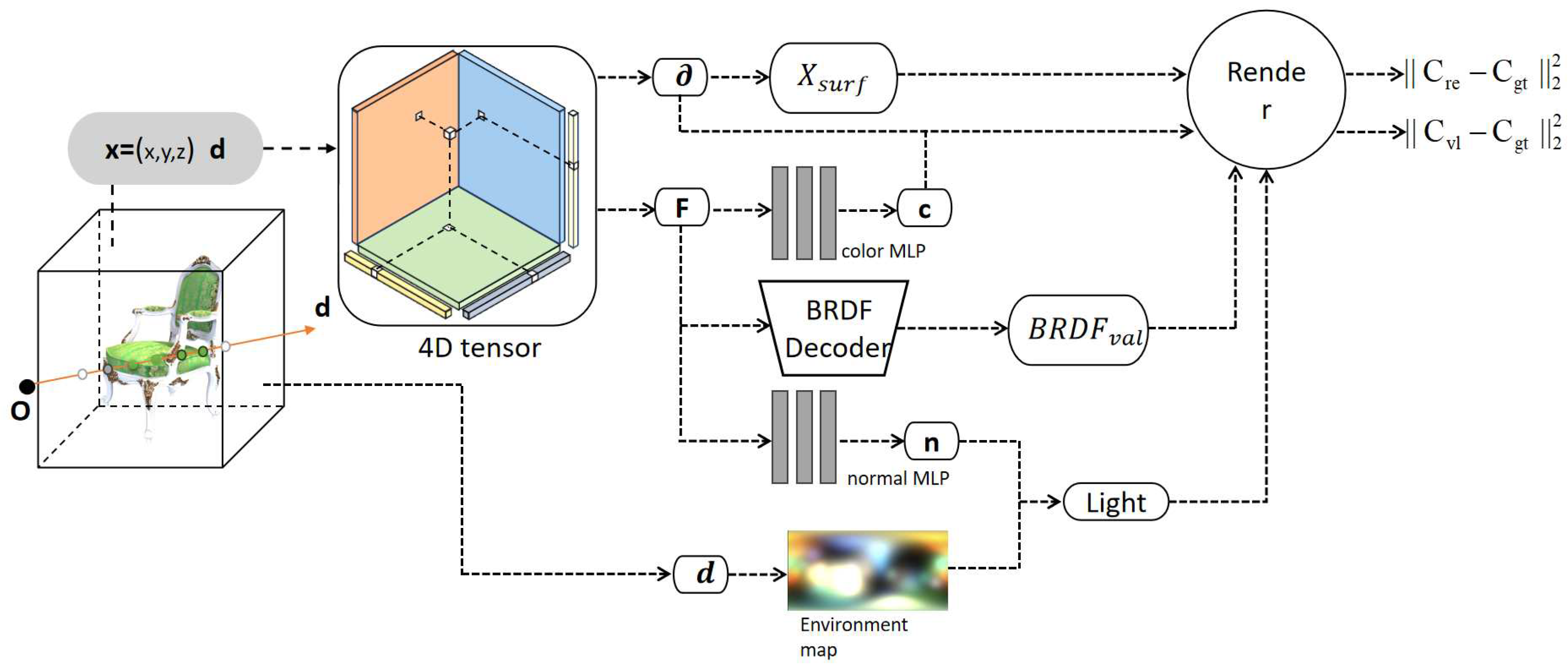
Figure 3.
Comparison of relighting result of two clothes scene between our method and the state-of-the-art techniques.
Figure 3.
Comparison of relighting result of two clothes scene between our method and the state-of-the-art techniques.
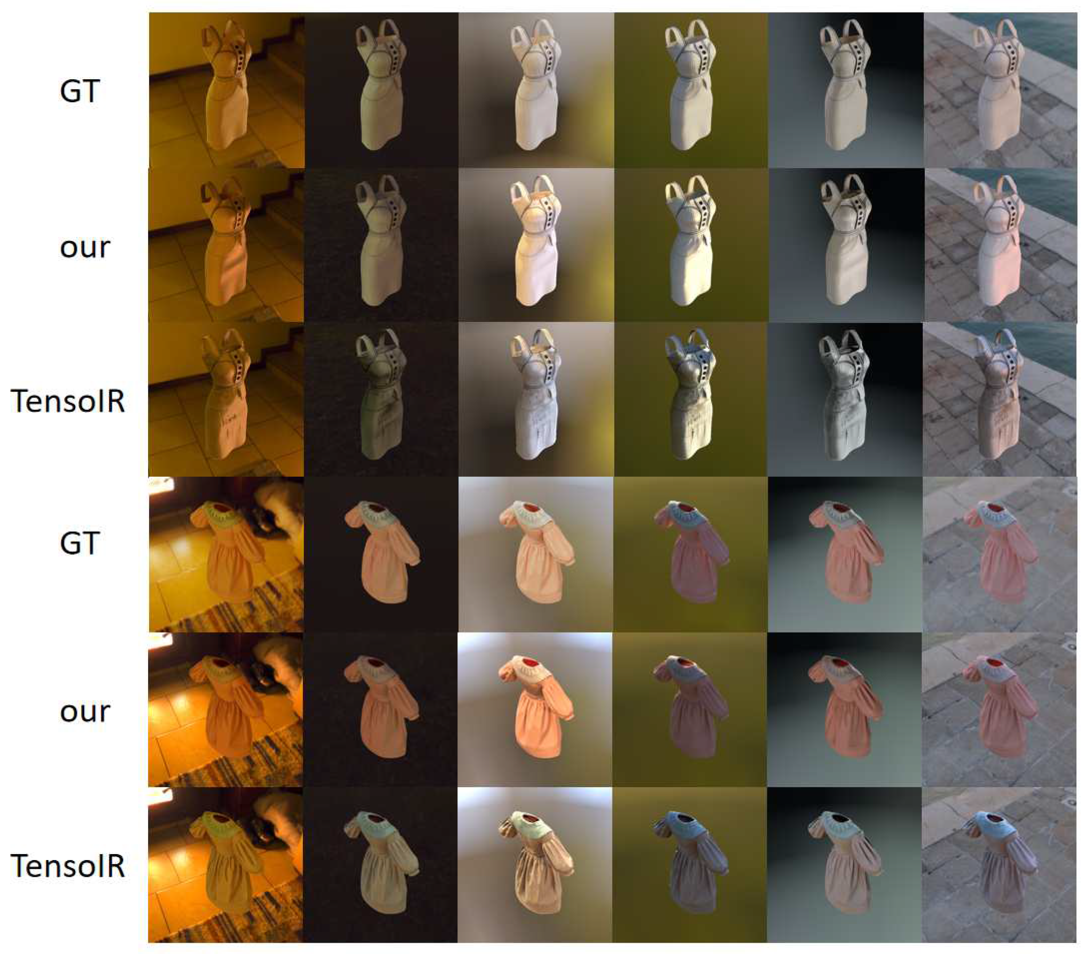
Figure 4.
Comparison of novel view of the LEGO scene and the corresponding surface normal results between our method and other state-of-the-art techniques.
Figure 4.
Comparison of novel view of the LEGO scene and the corresponding surface normal results between our method and other state-of-the-art techniques.
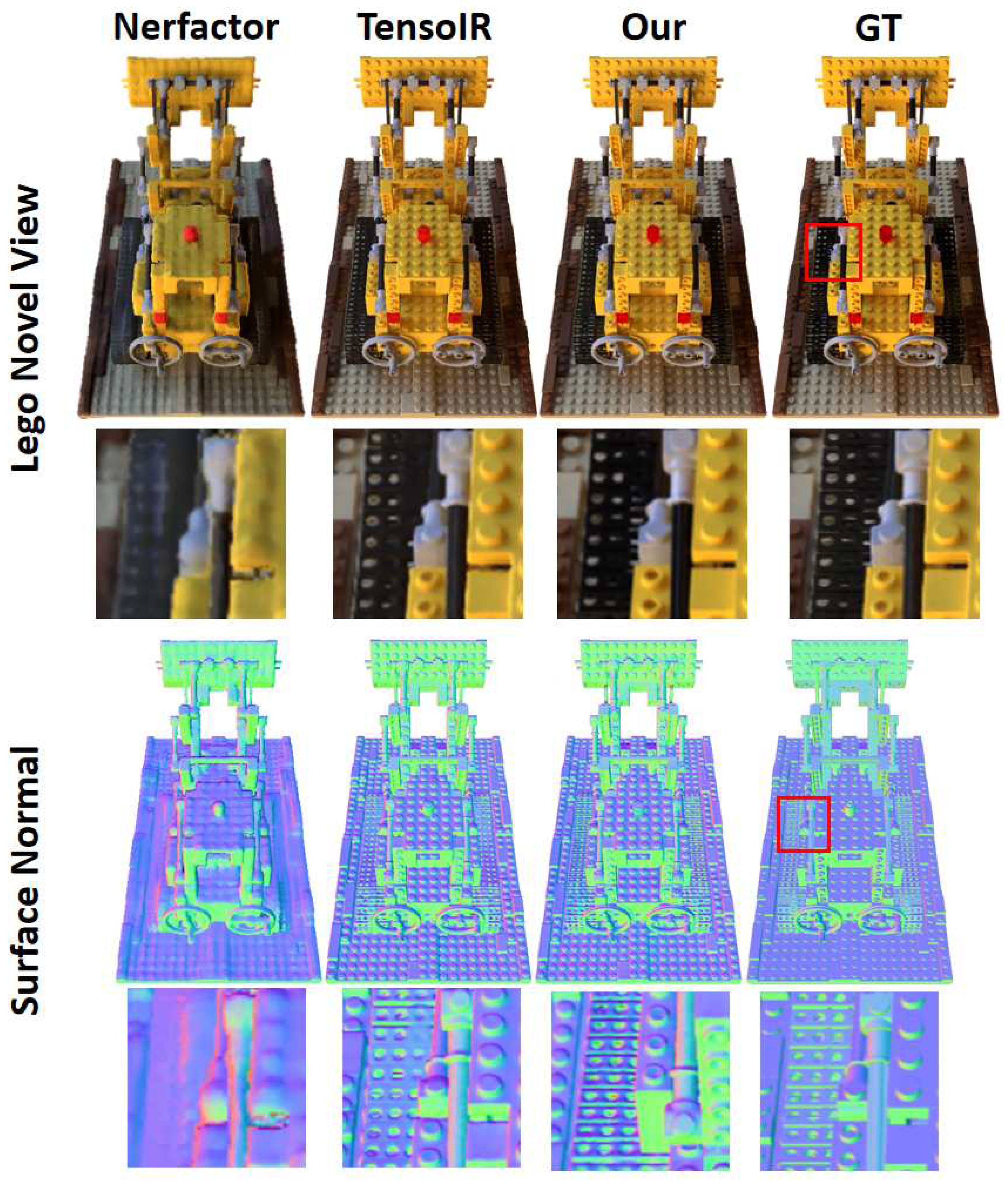

Table 1.
Conduct experiments on four synthetic datasets to quantitatively compare the results of new perspective synthesis, relighting, geometric surface normal estimation, and model training time across the four scenes.
Table 1.
Conduct experiments on four synthetic datasets to quantitatively compare the results of new perspective synthesis, relighting, geometric surface normal estimation, and model training time across the four scenes.
| Sence | Method | Nomal | Novel View Synthesis | Relighting | Training | ||||
|---|---|---|---|---|---|---|---|---|---|
| MAE↓ | PSNR↑ | SSIM↑ | LPIPS↓ | PSNR↑ | SSIM↑ | LPIPS↓ | Time↓ | ||
| Ficus | NeRFactor | 6.328 | 21.688 | 0.925 | 0.101 | 20.932 | 0.903 | 0.110 | 83.0hrs |
| TensoIR | 4.452 | 29.114 | 0.963 | 0.052 | 24.183 | 0.941 | 0.071 | 3.2hrs | |
| ours | 4.192 | 29.693 | 0.968 | 0.048 | 25.323 | 0.944 | 0.069 | 2.2hrs | |
| Lego | NeRFactor | 9.892 | 26.088 | 0.873 | 0.156 | 23.505 | 0.855 | 0.158 | 84.0hrs |
| TensoIR | 5.515 | 34.652 | 0.956 | 0.045 | 28.433 | 0.912 | 0.084 | 3.5hrs | |
| ours | 5.700 | 35.084 | 0.973 | 0.044 | 27.142 | 0.882 | 0.082 | 1.8hrs | |
| Armadillo | NeRFactor | 3.455 | 26.584 | 0.946 | 0.093 | 26.723 | 0.941 | 0.110 | 73.0hrs |
| TensoIR | 2.063 | 38.143 | 0.980 | 0.047 | 34.402 | 0.975 | 0.046 | 2.8hrs | |
| ours | 1.853 | 40.136 | 0.983 | 0.045 | 31.779 | 0.955 | 0.050 | 1.6hrs | |
| Hotdog | NeRFactor | 5.681 | 23.366 | 0.922 | 0.144 | 22.651 | 0.903 | 0.161 | 77.0hrs |
| TensoIR | 4.120 | 35.298 | 0.969 | 0.054 | 27.898 | 0.928 | 0.122 | 2.7hrs | |
| ours | 4.761 | 34.421 | 0.946 | 0.061 | 27.702 | 0.911 | 0.138 | 2.2hrs | |
| Average | NeRFactor | 6.339 | 24.432 | 0.917 | 0.124 | 23.453 | 0.901 | 0.135 | 79.3hrs |
| TensoIR | 4.038 | 34.302 | 0.967 | 0.050 | 28.729 | 0.939 | 0.081 | 3.1hrs | |
| ours | 4.127 | 34.834 | 0.968 | 0.049 | 27.987 | 0.923 | 0.085 | 2.0hrs | |
Note: The table highlights the best results in bold format, with an upward arrow indicating larger values are preferable, and a downward arrow indicating smaller values are preferable.
Table 2.
Comparison of experimental results of different BRDF decoders in the Ficus scene.
| Novel View Synthesis | Relighting | Training | ||||
|---|---|---|---|---|---|---|
| PSNR↑ | SSIM↑ | PSNR↑ | SSIM↑ | Time↓ | ||
| Ours decoder w/ E.F. | 28.864 | 0.952 | 26.578 | 0.949 | 5.6hrs | |
| Ours decoder w/ MLP | 29.693 | 0.968 | 25.323 | 0.944 | 2.2hrs | |
| Ours decoder w/ LSTM | 29.784 | 0.968 | 25.489 | 0.947 | 12.7hrs | |
Note: The table highlights the best results in bold format, with an upward arrow indicating larger values are preferable, and a downward arrow indicating smaller values are preferable.
Table 3.
Comparison of experimental results for the Ficus scene modeling using varying numbers of tensors.
Table 3.
Comparison of experimental results for the Ficus scene modeling using varying numbers of tensors.
| Novel View Synthesis | Relighting | Training | ||||
|---|---|---|---|---|---|---|
| PSNR↑ | SSIM↑ | PSNR↑ | SSIM↑ | Time↓ | ||
| Ours w/ A.M.F tensor | 29.231 | 0.962 | 25.217 | 0.942 | 4.3hrs | |
| Ours w/ A.S.F tensor | 29.622 | 0.968 | 25.339 | 0.944 | 3.2 hrs | |
| Ours | 29.693 | 0.968 | 25.323 | 0.944 | 2.2hrs | |
Note: The table highlights the best results in bold format, with an upward arrow indicating larger values are preferable, and a downward arrow indicating smaller values are preferable.
Disclaimer/Publisher’s Note: The statements, opinions and data contained in all publications are solely those of the individual author(s) and contributor(s) and not of MDPI and/or the editor(s). MDPI and/or the editor(s) disclaim responsibility for any injury to people or property resulting from any ideas, methods, instructions or products referred to in the content. |
© 2024 by the authors. Licensee MDPI, Basel, Switzerland. This article is an open access article distributed under the terms and conditions of the Creative Commons Attribution (CC BY) license (https://creativecommons.org/licenses/by/4.0/).
Copyright: This open access article is published under a Creative Commons CC BY 4.0 license, which permit the free download, distribution, and reuse, provided that the author and preprint are cited in any reuse.


