Submitted:
08 January 2024
Posted:
09 January 2024
You are already at the latest version
Abstract
Breast cancer is the most common cause of mortality due to cancer for woman both in Lithuania and worldwide. Chances of survival after diagnosis differ significantly depending on the stage of disease at the time of diagnosis and other factors. One way to estimate survival is to construct a Kaplan-Meier estimate for each factor value separately. However, in cases when it is impossible to observe a large number of patients (for example, in case of countries with lower numbers of inhabitants) dividing data into subsets, say, by stage at diagnosis may lead to results where some subsets contain too little data so that results of Kaplan Meier (or any other) method will become statistically incredible. The problem may become even more acute if the researcher would like to use more risk factors, such as stage at diagnosis, sex, place of living, treatment method, etc. Alternatively, Cox models are used to analyse survival data with covariates, and they don’t require dividing the data into subsets according to chosen risks factors (hazards).
Keywords:
breast cancer
; central death rate
; exposure to risk
; Kaplan – Meier estimate
; survival analysis
; stratified Cox model
; cancer awareness campaign
MSC: 62P05; 91G05
1. Introduction
The breast cancer is one of most the common women cancer, despite the fact that incidence and mortality rates may differ significantly in different countries. For example, in USA breast cancer amounts to of all new female cancers each year, see [1], while worldwide breast cancer is the most commonly diagnosed cancer type, accounting for 1 in 8 new cancer diagnoses, see [2]. More statistics about morbidity and mortality worldwide can be found in [3] and in references therein.
Despite advances in medicine and preventive diagnostics, which allow cancer to be detected at an earlier stage and treated with modern therapies, cancer deaths remain the second leading cause of mortality among women in Lithuania. So, in 2022 deaths due to cancer amounted to of all deaths among females of all ages, while in 2018 the share of deaths due to cancer was . Even during 2020 when the Covid-19 pandemic began of all females died due to cancer and "only" due to Covid-19. Only during 2021 cancer became third cause of death among females () when Covid-19 temporarily became second one (). For more statistics interested readers are referred to [4].
It is not surprising that a significant amount of research is conducted to estimate survival after the cancer diagnosis. Survival depends very much on the stage at diagnosis as well as other factors (comorbidities, treatment received, etc.). The Kaplan-Meier estimate remains one of the most popular tools for analysis of survival after diagnosis. Interested readers may find many publications on application of Kaplan-Meier for estimation of future lifetime after breast cancer diagnosis. For example, Narod et al. [5] used the Kaplan-Meier technique and time to death histograms to estimate mortality of women who died due to breast cancer during the 20 year period after diagnosis. Fisher et al. [6] analyzed survival among breast cancer patients based on treatment received. Giordano et.al. [7] analyzed possible improvements in survival after diagnosis of breast cancer.
Skucaite et al. [8] analysed survival after breast cancer diagnosis among Lithuanian females. Authors of the paper applied Kaplan-Meier procedure to obtain survival rates and then fitted appropriate analytic functions to the obtained estimates. This way allowed to obtain estimation of survival for longer period. Surely, there are much more publications on similar matters because the Kaplan-Meier method is relatively simple to use and to obtain estimates of survival functions, see for instance [9,10,11,12,13,14]. However, if we are interested in how mortality (survival) depends on various hazards (risk factors), then all observations need to be divided into subgroups (strata) and the Kaplan-Meier procedure is applied to each subset separately.
To avoid the problem of dividing data into subsets, researchers may use the Cox proportional hazards method. This method is widely used to model survival after diagnosis depending on various risk factors (hazards). For instance in [15,16,17,18], the Cox proportionate hazards method is used for survival analysis. An interesting approach is given by Putter et al. [19], where the authors suggest the way how to deal with time dependent variables when using the Cox model for survival analysis among lung cancer patients.
Recently, many studies have been conducted on the survival of patients with breast cancer. Statistical survival studies are conducted in order to determine the danger of this critical disease, compare treatment methods, and determine the effectiveness of health care in a given country, see [20,21,22,23,24] for instance.
In this paper we identify the main hazards (factors) that may influence survival chances after breast cancer is diagnosed. Firstly, we obtain Kaplan-Meier estimates and then use the stratified Cox model to determine impact of some potential hazards, such as stage at inception, circumstance of diagnosis and calendar year of diagnosis to survival probabilities.
The rest of our paper is organized as follows. In Section 2, we present some mathematical preliminaries and notations which we use later as well as mathematical basis of Kaplan-Meier and the stratified Cox models. In Section 3, we describe data and methods used for our analysis. Main results of our analysis are presented in Section 4. The possible applications of our research are discussed in the concluding Section 5.
2. Some notations and mathematical preliminaries
Consider a person who has just been diagnosed with cancer. Her future lifetime is a nonnegative random variable which we define by T. We assume that survival function of lifetime T
is absolutely continuous.
As usual, we denote by the probability to survive until time for individual being alive at time t by
Alternatively, probability to die until time being alive at time t is defined by equality
The instantaneous rate of mortality, the so called hazard rate at time t, or the force of mortality at time t, is defined by the following equality
which makes sense because the survival function S is supposed to be absolutely continuous.
Sometimes it is useful to average behaviour of the force of mortality in the interval . In such a case, central death rate (central mortality rate) in the interval , which is defined as weighted arithmetic average of force of mortality, is used:
Finally, we define measure of risk exposure, central exposure to risk, which is measured as total number of years lived by persons under investigation in the interval and defined as . Assume that – number of deaths during the period of , then central death rate may be estimated using ratio:
2.1. Kaplan-Meier estimate
Kaplan-Meier estimate may be used to estimate survival probabilities. Main advantages of this method are presented in [25] and in references therein:
- Kaplan-Meier estimate is suitable for data sets with a limited number of cases, otherwise using this method may become time consuming. For our data we used Excel spreadsheet and R software environment for this reason.
- Kaplan-Meier estimate is very suitable for medical trials when time since inception of disease is more important than solely age of patient, so it is difficult to apply standard actuarial procedures used for construction of life table.
- Kaplan-Meier estimate is non-parametric, so no advance assumption about functional parametric form of survival function is required neither parameters need to be estimated. Despite being non-parametric, the estimator is still statistical estimator, hence the standard error and confidence intervals can be calculated.
- Kaplan-Meier estimate is used for death probability ; interval h can be as short as one day, e.g. . So, Kaplan-Meier estimate is suitable for estimation of death probabilities during quite short period without making any assumptions about distribution of deaths (form of survival function S) within one year. Moreover, interval h may differ for different subintervals and is not determined a priori by analyst but is based on data under investigation, so h is determined a posteriori.
In short, the observation interval is divided into subintervals by partitioning it at each point where a death occurs. Estimate of the survival function S is then obtained using formula:
where is the number of deaths occurred at time and is the number of patients under observation alive immediately before time .
For the estimate , it is possible to calculate the approximate standard error using the Greenwood formula:
2.2. Cox models
In most cases, we will observe several hazards that may affect the risk of dying. For example, when analyzing mortality in the case of a breast cancer diagnosis, the time since diagnosis may be considered the primary factor, but the stage at diagnosis, the year of diagnosis, and the patient’s age at diagnosis may also significantly influence the risk of dying. We will call such hazards covariates. In this case it is possible to divide all data into subsets according to chosen covariates, for example, divide all data into subsets according to the stage at inception. Kaplan-Meier estimates are then repeated for each subset, producing different survival functions for each subset. The advantage of such data stratification is, by no means, simplicity. However, if the number of subsets is bigger, the procedure may become time consuming. Moreover, it may happen that some subsets will include quite small number of deaths, so statistical analysis of such subsets will become meaningless.
An alternative way to such data stratification is to include covariates in the model of hazard rate (force of mortality). For instance, suppose we are interested how two discrete covariates may affect mortality after diagnosis, mainly
- Stage at inception, labelled 1 through 4, according to stage of cancer at diagnosis.
- Circumstances of diagnosis, labelled 0, if patient was examined on her initiative or 1, if cancer was detected during Cancer Awareness program.
In this case, for every observed individual i we define the covariate vector
and hazard rate (force of mortality) for individual i becomes function of the covariates as well as time since diagnosis:
2.2.1. Proportional hazards model
We consider the general case and denote covariate vector for i-th individual by , where m is number of covariates. Then, according to proportional hazard model, we suppose that force of mortality has the following form:
where are real coefficients.
The first factor is a function of time since diagnosis only which is called baseline hazard. In usual actuarial practice, baseline hazard is also a function of age x, see [28], for instance. However, in our case, it is more natural to define baseline hazard as function of time since diagnosis only. The second factor
depends on covariates of i-th individual, but not on time. Coefficients and baseline hazard should be found (estimated) from data.
So, hazard rates for two individuals, say i and j, are supposed to be in the same proportion at all times t, namely
Regression coefficients may be found by maximizing partial likelihood function. To estimate baseline hazard function researcher usually needs to make assumption that baseline hazard follows some know parametric law of mortality, say, Gompertz. Alternatively, if researcher is interested in only effect of covariates, baseline hazard may not be estimated since it cancels out, as may be seen from (2). Cox model is quite well known example of the latter approach, see [29].
Assumption of proportionality should be tested. This may be done, for example, using method of Schoenfeld residuals, see [30], for instance. If this assumption does not hold, stratified Cox model may be used, however, results should be interpreted with great care.
2.2.2. Stratified Cox model
If some covariates do not follow assumption of proportionality, then stratified Cox model may be used. Under such approach, all data under consideration are divided into strata based on hazards that do not meet the proportionality assumption. However, calculations are not done separately for each strata, instead partial likelihood function is constructed by multiplying likelihood functions for each strata. So, problem that some strata will contain to little data is avoided.
3. Data and calculations
Data collected by the Lithuanian Cancer Registry (www.nvi.lt) was used for our analysis. We analyzed only cases when patient was diagnosed with cancer for the very first time, i.e. there was no evidence that patient was diagnosed any type of cancer before.
We analyzed cases diagnosed during the period of 1995 – 2016 and observed all lives since inception of disease until death or until December 31, 2021, if earlier. Cases lost in follow up were treated as right censored, e.g. survival time for such persons was considered to be at least as long as last day of their observation. The same approach was adopted when treating all survivals until end of study period, namely, December 31, 2021, i.e. survival time for those cases is known to be as long as end of study period. It is important to note that even patients diagnosed at the end of diagnostic period, e.g. the end of 2016, had the chance to survive at least 5 years. We disregarded the reason of death after diagnosis since we assumed that all deaths after diagnosis are due to cancer, or at least diagnosis accelerated death.
We had initial set of 30479 cases. After the initial inspection, we decided to exclude 102 cases where the date of death coincided with the date of diagnosis. Most of these cases were situations where the cause of death on the Death certificate was "breast cancer". Thus, such patients were diagnosed earlier than the death, but it is not possible to track survival time from the moment of diagnosis until death. We also removed 1750 cases where stage of disease was not recorded. Finally, since 2008 cancer in different breasts (left and right) are considered as two separate diseases. We observed 520 pairs where two diseases were recorded for the same patient and removed cases with the later date of diagnosis. So, final set of data consisted of 28107 records (N=28107).
Deaths that occurred later than 5 years after diagnosis were disregarded since we were interested in survival up to 5 years, so all such records were treated as censored data.
We analysed three main hazard factors, stage at inception (1 through 4), circumstances of diagnoses (Cancer Awareness program vs examination on patient’s initiative) and year of diagnosis.
It is obvious that stage at inception may influence survival significantly with lower survival related to higher stage. Additionally, we assumed that Cancer Awareness programs help diagnose the disease at earlier stages, while patients applying to medical office on their own initiative may already experience some of the symptoms that indicate that the stage of the disease may be higher. Only about 4% of patients in our study were diagnosed during Cancer Awareness program, nevertheless we decided to treat this as hazard. We will use term Cancer Awareness program to define both medical check-up due to participation in Cancer Awareness program or just routine regular medical check-up. We also assumed that year of diagnosis may have a positive effect on survival due to general advance in diagnosis and treatment. So, we used two data intervals: year 1995 through 2004 and year 2005 through 2016.
4. Main results
Main results of our analysis are described in this section. We start from the Kaplan-Meier estimate and then continue with (stratified) Cox method.
4.1. Kaplan-Meier estimate
We used the Kaplan-Meier method to analyse survival after diagnosis according to risk (hazard) group: stage at inception (1 through 4), circumstance of diagnosis (Cancer Awareness Program vs patient’s initiative) and period of diagnosis (1995 through 2004 vs 2005 through 2016).
Main results are summarized in Table 1. We note that data were right censored, i.e. maximum period of observation was 60 months after diagnosis. Hence the average of the future lifetime and median of the future lifetime after diagnosis were estimated under condition that maximum observed period of survival was 60 months.
As may be expected, the stage at inception has negative impact on survival. Patients diagnosed with Stage 1 may expect that their average survival period will be more than twice longer compared to patients diagnosed with Stage 4. Other hazards did not lead to such significant differences in average survival. However, patients diagnosed during Cancer Awareness program had a bit longer average survival time compared to those checked up at their initiative. Later period of diagnosis also had slightly positive impact on survival.
We constructed estimate of survival function using Kaplan-Meier method. The log-rank test showed a statistically significant difference in survival according to the different stages at inception. Probability to survive 5 years for patients diagnosed with Stage 1 is slightly more than 90%, while chances for those diagnosed with Stage 4 are slightly less than 14%. These results are very much in line with those obtained in [8]. For more details, please see Table 2 and Figure 1.
Log rank test showed statistically significant differences in survival by circumstance of diagnosis with poorer survival of those patients who were checked up at their initiative. They had 66% chance to survive 5 years compared to slightly more than 80% survival after diagnosis obtained due to participation in Cancer Awareness Programs (CAPs). However, these results should be interpreted with care since only about 4% patients were diagnosed during CAPs. Moreover, it is obvious that better survival is influenced not by the way how diagnosis was obtained (CAPs vs patient’s initiative), but rather by the fact that usually those who participated in CAPs were diagnosed with lower stages, which leads to better survival experience. Readers may see from Table 3 that percentage of patients diagnosed with stage 1 or 2 during CAPs amount to 86% compared to 67% of cases diagnosed during inspection by patient’s initiative. The most life-threatening stage 4 was diagnosed for only 3% of patients who participated in the CAPs, compared to 11% of patients examined due to their initiative. Our results show that it is worth investing in CAPs, since they may increase the chances of being diagnosed at an earlier stage. Considering differences in life expectancy after diagnosis, the cost of treatment and the cost of temporary disability due to disease, CAPs can not only help to prolong life span of patients but also have a positive impact on public finances.
Log-rank test also showed statistically significant differences in survival by period of diagnosis. Poorer 5 year survival was observed for earlier period (1995 - 2004). Patients diagnosed later (2005 - 2016) had about 22 % higher probability to survive 5 years compared to patients diagnosed during the period of 1995-2004. This may be due to several reasons, the main ones being advances in medicine and the introduction of CAPs. CAPs were started in Lithuania during the period of 2002 - 2004 and probably led to more cases being diagnosed at earlier stages (see Table 4). Advances in medicine probably led to better survival experience after diagnosis due to the new treatment methods.
4.2. Cox models
Since there are four possible stages of the disease and stages are measured using ordinal scale, we used 3 dummy variables for stages 2 through 4 when defining force of mortality, see equation (1). Each dummy variable may take value 1 if corresponding stage was diagnosed or value 0 otherwise. We do not define dummy variable for stage 1, since stage 1 is diagnosed if all three other dummy variables take value 0. Stage 1 is considered to be baseline hazard level.
For other two hazards we proceeded as follows:
If the value of a particular hazard is 0, it is considered to be the baseline hazard level and hazard ratios are calculated with respect to the baseline hazard level.
4.2.1. Univariate Cox model
We started analysis by applying the univariate Cox model, i.e. we constructed force of mortality function (1) for each hazard factor separately, see Table 5.
Our analysis showed that stage at diagnosis significantly increases the risk of death. Compared to stage 1, diagnosis of stage 2 increases the risk of dying about 2.65 times, because the hazard rate estimate . While stage 3 and stage 4 increases the risk of dying by 7.62 and 23.55 times respectively.
Patients who were diagnosed during CAPs have lower risk of dying by () times compared to patients examined on their initiative. However, it should recall that usually lower stages of cancer are found during examination via CAPs, see Table 3. This result is in line with the result presented in the previous section, see Figure 2.
Later period (2005 - 2016) of diagnosis decrease the risk of dying by 1.63 times () compared to the earlier period of diagnosis (1995 - 2004). This result is also in line with the result stated in the previous section, see Figure 3.
The Wald statistics showed that impact of all hazards is statistically significant. For more results, please refer to the Table 5. However, we should keep in mind that results of univariate Cox model should be interpreted with care since Schoenfeld test showed that all three covariates most likely fail to fulfil the proportionality assumption.
4.2.2. Multivariate Cox model
We constructed multivariate Cox model using all three covariates, see equation (1). Recall that the hazard rates of two randomly selected individuals should remain in constant proportion all the time, see equation (2). We used Schoenfeld test again to test assumption of proportionality. Covariate Stage at inception failed to fulfil this assumption, however, other two covariates most likely fulfil the assumption of proportionality. Therefore, we stratified data set by dividing it into four strata based on stage at diagnosis and applied stratified Cox model. Recall that stratified Cox model allows to perform calculations for all data at once, so we avoided the problem that some strata may contain too little data.
4.2.3. Stratified Cox model
We found that covariates Circumstance and Period of diagnosis remain statistically significant. Both diagnosis due to Cancer Awareness program and later period of diagnosis have a positive impact on survival. Analysis, presented in Table 6, shows that diagnosis stated during participation in CAP may reduce the risk of dying by 1.31 times (=0.763), while the later period of diagnosis reduces the risk of dying by 1.25 time (=0.802). Reduction in mortality is independent of the stage at diagnosis, however, baseline hazard from equality (1) can be different for different stages of disease. Thus, differences in survival between stages will depend not only on the hazard rates, but also on the baseline hazard function. However, we did not made any assumption about the function of baseline hazard and therefore did not estimate it.
5. Concluding Remarks
We examined survival after breast cancer diagnosis among Lithuanian females. As might be expected, the stage of the disease is a very important hazard factor. Higher stages of the disease decrease life expectancy quite significantly. We examined two more hazards, circumstance of diagnosis and period of diagnosis. We found that better survival is observed if the examination of patient was carried out during Cancer awareness program (CAP) and disease is diagnosed during later period. However, CAPs increase the chances of being diagnosed at an earlier stage. On the other hand, later period of diagnosis increases the chances that the patient was examined during CAPs, as such programs were introduced in Lithuania during the period of 2002-2004. Better survival is more likely due to the earlier stage of the disease rather than participation in CAPs or the later period of diagnosis. Our results are in line with those obtained in [18], where authors state that: The main factor causing low survival time was because the patient comes for treatment already in an advanced stage even accompanied by comorbidities (such as diabetes, anemia and hypertension).
One suggested direction for further studies can be a detailed analysis of co-morbidities as potential hazards, since existing diseases may indicate that women are at a higher risk of being diagnosed with breast cancer and/or may have a greater risk of experiencing negative treatment outcomes.
Unfortunately, in Lithuania, the breast cancer screening program is still not effective, the percentage of participation in 2022 was only 26.6 percent (see [33] (in Lithuanian), [34] and references therein). The survival rates for breast cancer in Lithuania are among the worst in the world (see [35]). It is necessary to find measures and political solutions to increase the efficiency of the CAPs in Lithuania. Early detection of breast cancer may lead to significant positive impact on survival rates and better quality of life after treatment.
Author Contributions
Conceptualization, J.Š. and I.V.; methodology, A.S. and J.L.; software, J.L.; validation, A.S. and I.V.; formal analysis, J.Š.; investigation, J.L. and A.S.; writing-original draft preparation, A.S.; writing-review and editing, J.Š. and I.V.; visualization, J.L.; supervision, J.Š.; project administration, A.S.; funding acquisition, J.Š. All authors have read and agreed to the published version of the manuscript.
Funding
Not applicable.
Institutional Review Board Statement
Not applicable.
Informed Consent Statement
Not applicable.
Data Availability Statement
The data collected by Lithuanian Cancer Registry are used for our analysis. Lithuanian Cancer Registry is a nationwide and population based cancer registry which covers the whole territory of Lithuania. Ethical approval for the analysis of the aggregated and anonymized data was not required.
Conflicts of Interest
The authors declare no conflict of interest.
References
- American Cancer Society, https://www.cancer.org/cancer/types/breast-cancer/about.html, accessed July 5, 2023.
- The International Agency for Research on Cancer of the World Health Organization, https://www.iarc.who.int/news-events/current-and-future-burden-of-breast-cancer-global-statistics-for-2020-and-2040/, accessed July 5, 2023.
- Arnold, M.; Morgan, E.; Rumgay, H.; Mafra, A.; Singh, D.; Laversanne, M.; Vignat, J.; Gralow, J.R.; Cardoso, F.; Siesling, S.; et al. Current and future burden of breast cancer: Global statistics for 2020 and 2040. The Breast 2022, 66, 15–23. [Google Scholar] [CrossRef] [PubMed]
- Institute of Hygiene. Causes of Death Registry (in Lithuanian), https://www.hi.lt/en/mortality-in-lithuania.html, accessed August 4, 2023.
- Narod, S.A.; Giannakeas, V.; Sopik, V. Time to death in breast cancer patients as an indicator of treatment response. Breast Cancer Res. Treat. 2018, 172, 659–669. [Google Scholar] [CrossRef] [PubMed]
- Fisher, S.; Gao, H.; Yasui, Y.; Dabbs, K.; Winget, M. Survival in stage I-III breast cancer patiens by surgical treatment in a publicly funded health care system. Ann. Oncol. 2015, 26, 1161–1169. [Google Scholar] [CrossRef] [PubMed]
- Giordano, S.H.; Buzdar, A.U.; Smith, T.L.; Kau, S.W.; Yang, Y.; Hortobagyi, G.N. Is breast cancer survival improving? Cancer 2004, 100(1), 44–52. [Google Scholar] [CrossRef] [PubMed]
- Skučaitė, A.; Puvačiauskienė, A.; Puišys, R.; Šiaulys, J. Actuarial analysis of survival among breast cancer patients in Lithuania. Healthcare 2021, 9, 383. [Google Scholar] [CrossRef] [PubMed]
- Kaplan, E.L.; Meier, P. Nonparametric estimation from incomplete observations. J. Am. Stat. Assoc. 1958, 53, 457–481. [Google Scholar] [CrossRef]
- Meier, P. Estimation of a distribution function from incomplete observations. J. Appl. Probab. 1975, 12, 67–87. [Google Scholar] [CrossRef]
- Meier, P.; Karrison, T.; Chapell, R.; Xie, H. The price of Kaplan-Meier. J. Am. Stat. Assoc. 2004, 99, 890–896. [Google Scholar] [CrossRef]
- Staudt, Y.; Wagner, J. Factors driving duration to croos-selling in non-life insurance: new empirical evidence from Switzerland. Risks 2022, 10, 187. [Google Scholar] [CrossRef]
- Tholkage, S.; Zheng, Q.; Kulasekera, K.G. Conditional Kaplan-Meier estimator with functional covariates for time-to-event data. Stats 2022, 5, 1113–1119. [Google Scholar] [CrossRef]
- Nemes, S. Asymptotic relative efficiency of parametric and nonparametric survival estimators. Stats 2023, 6, 1147–1159. [Google Scholar] [CrossRef]
- Arsyad, R.; Thamrin, S.A.; Jaya, A.K. Extended Cox model for breast cancer survival data using Bayesian approach: A case study. J. Phys. Conf. Ser. 2019, 1341, 092013. [Google Scholar] [CrossRef]
- Lin, R.H.; Lin, C.S.; Chuang, C.L.; Kujabi, B.K.; Chen, Y.C. Breast cancer survival analysis model. Appl. Sci. 2022, 12(4), 1971. [Google Scholar] [CrossRef]
- Pereira, L.C.; Silva, S.J.; Fidelis, C.R.; Brito, A.L.; Xavier Júnior, S.F.A.; Andrade, L.S.S.; Oliveira, M.E.C.; Oliveira, T.A. Cox model and decision trees: an application to breast cancer data. Rev. Panam. Salud. Publica 2022, 46, e17. [Google Scholar] [CrossRef] [PubMed]
- Bustan, M.N.; Arman; Aidid, M.K.; Gobel, F.A.; Syamsidar. Cox proportional hazard survival analysis to inpatient breast cancer cases. J. Phys. Conf. Ser. 2018, 1028, 012230. [Google Scholar] [CrossRef]
- Putter, H.; Sasako, M.; Hartgrink, H.H.; Velde, C.J.H.; Houwelingen, J.C. Long-term survival with non-proportional hazards: results from the Dutch Gastric Cancer Trial. Stat. Med. 2005, 24, 2807–2821. [Google Scholar] [CrossRef]
- Akezaki, Y.; Nakata, E.; Kikuuchi, M.; Sugihara, S.; Katayama, H.; Hamada, M.; Ozaki, T. Association between overall survival and activities of daily living in patients with spinal bone metastases. Healthcare 2022, 10, 350. [Google Scholar] [CrossRef] [PubMed]
- Haussmann, J.; Budach, W.; Nestle-Krämling, C.; Wollandt, S.; Tomaskovich, B.; Corradini, S.; Bölke, E.; Krug, D.; Fehm, T.; Ruckhäberle, E.; et al. Predictive factors of long-term survival after neoadjuvant radiotherapy and chemotherapy in high-risk breast cancer. Cancers 2022, 14, 4031. [Google Scholar] [CrossRef] [PubMed]
- Rim, C.H.; Lee, W.J.; Musaev, B.; Volichevich, T.Y.; Pozlitdinovich, Z.Y.; Lee, H.Y.; Nigmatovich, T.M.; Rim, J.S. Comparison of breast cancer and cervical cancer in Uzbekistan and Korea: The first report of the Uzbekistan-Korea onkology consortium. Medicina 2022, 58, 1428. [Google Scholar] [CrossRef]
- Gwak, H.; Woo, S.S.; Oh, S.J.; Kim, J.Y.; Shin, H.C.; Youn, H.J.; Chun, J.W.; Lee, D.; Kim, S.H. A comparison of the prognostic effects of fine needle aspiration and core needle biopsy in patients with breast cancer: A nationwide multicenter prospective registry. Cancers 2023, 15, 4638. [Google Scholar] [CrossRef]
- Zhang, S.; Liu, Y.; Liu, X.; Liu, Y.; Zhang, J. Prognoses of patients with hormone receptor-positive and human epidermal growth factor receptor 2-negative breast cancer receiving neoadjuvant chemotherapy before surgery: A restrospective analysis. Cancers 2023, 15, 1157. [Google Scholar] [CrossRef] [PubMed]
- Macdonald, A.S.; Richards, S.J.; Currie, I.D. The Kaplan-Meier estimator, in Modelling Mortality with Actuarial Applications, eds Ch. Daykin and A. Macdonald; Cambridge University Press, Cambridge, 2018, p. 134 - 140.
- London, D. Survival Models and their Estimation; ACTEX Publications, Winsted, Connecticut, 1988.
- Kleinbaum, D. G.; Klein, M. Survival Analysis. A Self Learning Text (Second Edition); Springer Science+Business Media, LLC, 2005, p. 45 - 73.
- Macdonald, A.S.; Richards, S.J.; Currie, I.D. Example: a proportional hazard model, in Modelling Mortality with Actuarial Applications, eds Ch. Daykin and A. Macdonald; Cambridge University Press, Cambridge, 2018, p. 122-124.
- Macdonald, A.S.; Richards, S.J.; Currie, I.D. The Cox Model, in Modelling Mortality with Actuarial Applications, eds Ch. Daykin and A. Macdonald; Cambridge University Press, Cambridge, 2018, p. 124-125.
- Lee, T.L.; Wang, J.W. Statistical methods for survival data analysis, 4-th ed; Wiley, New Jersey, 2013.
- CRAN – Package survival, https://cran.r-project.org/web/packages/survival/index.html, accessed May 26, 2022.
- CRAN – Package survminer, https://cran.r-project.org/web/packages/survminer/index.html, accessed May 26, 2022.
- National Health Insurance Fund under the Ministry of Health, https://ligoniukasa.lrv.lt/lt/veiklos-sritys/informacija-gyventojams/ligu-prevencijos-programos, accessed December 5, 2023.
- Steponavičienė, L.; Briedienė, R.; Vansevičiūtė-Petkevičienė, R.; Gudavičienė-Petkevičienė, D.; Vincerževskienė, I. Breast Cancer Screening Program in Lithuania: Trends in Breast Cancer Mortality Before and During the Introduction of the Mammography Screening Program. Acta Med. Litu. 2020, 7, 61–69. [Google Scholar] [CrossRef] [PubMed]
- Allemani, C.; Matsuda, T.; Di Carlo, V.; Harewood, R.; Matz, M.; Nikšić, M.; Bonaventure, A.; Valkov, M.; Johnson, C.J.; Estève, J.; et al. CONCORD Working Group. Global surveillance of trends in cancer survival 2000-14 (CONCORD-3): analysis of individual records for 37 513 025 patients diagnosed with one of 18 cancers from 322 population-based registries in 71 countries. Lancet 2018, 391, 1023–1075. [Google Scholar] [CrossRef] [PubMed]
Figure 1.
Estimation of survival by stage at diagnosis.
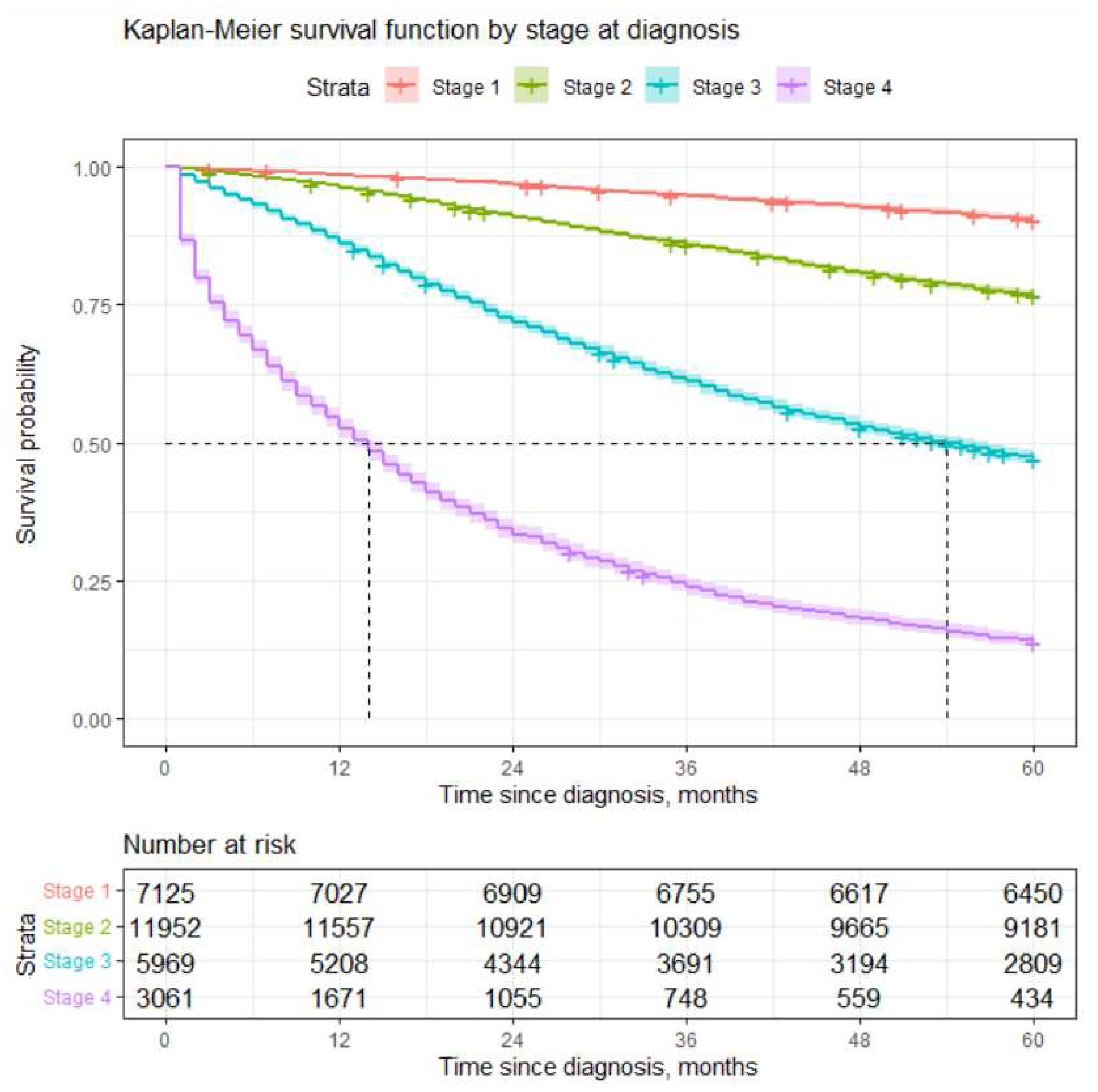
Figure 2.
Estimation of survival by circumstance of diagnosis.
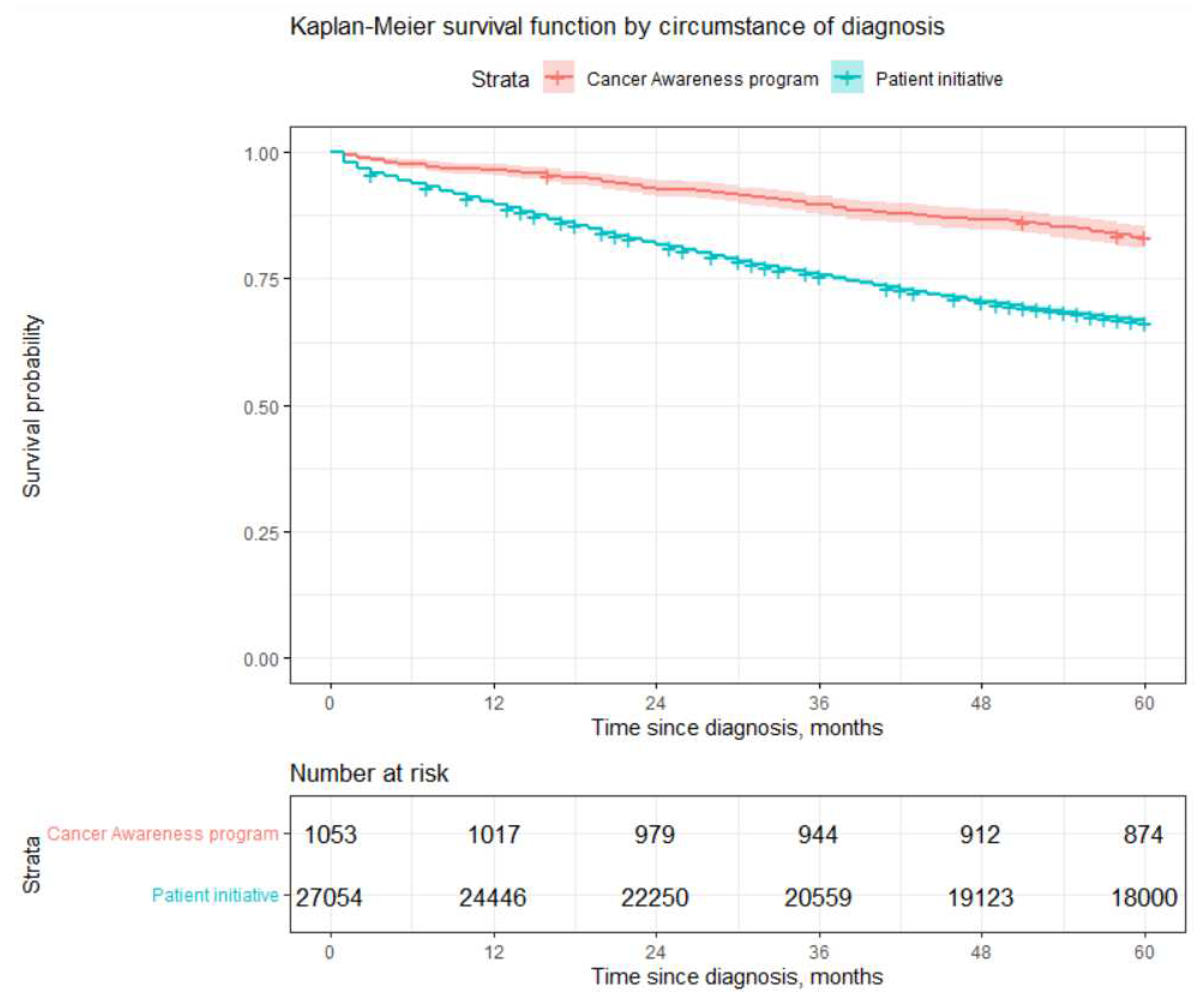
Figure 3.
Estimation of survival by period of diagnosis.
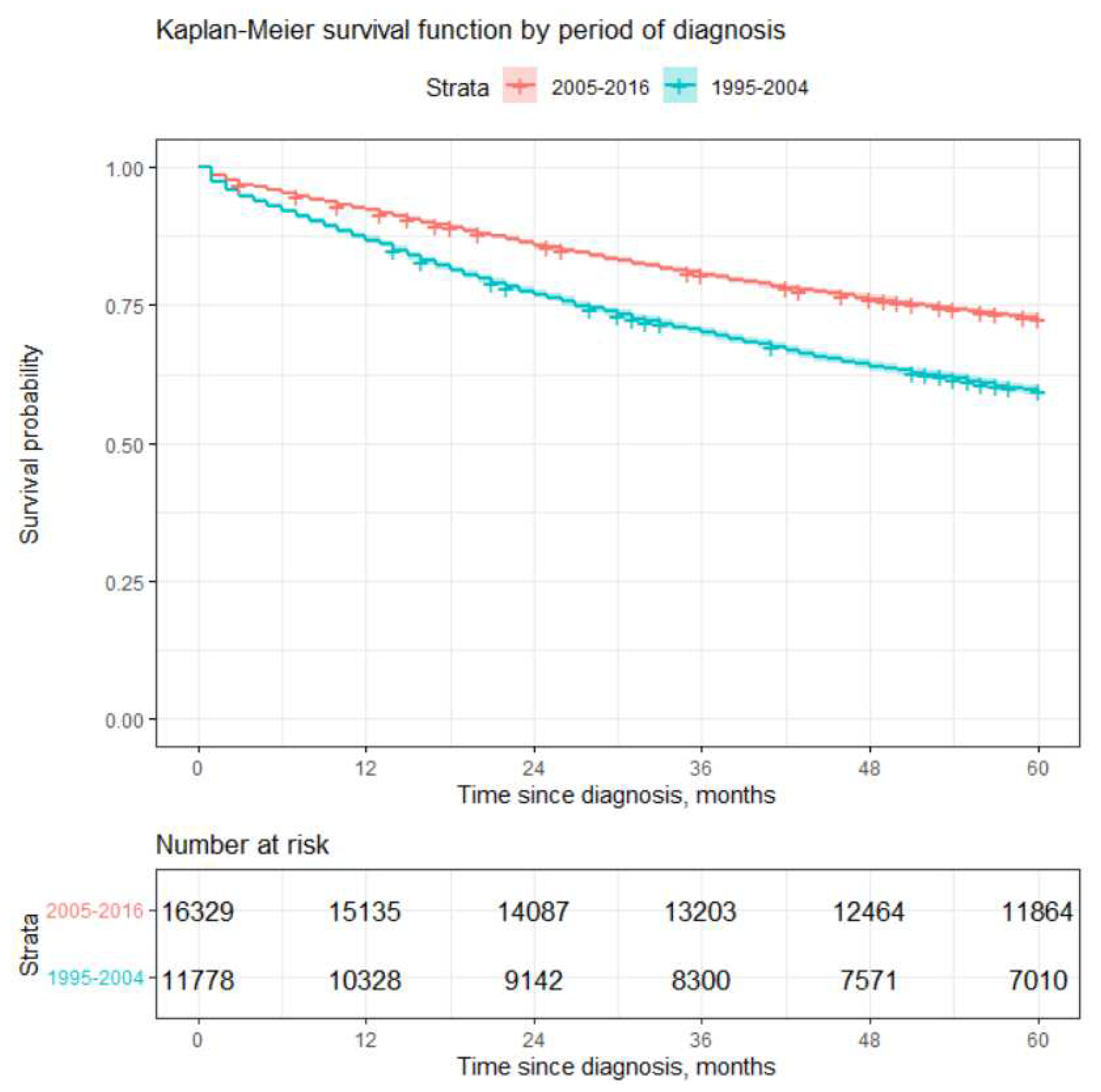

Table 1.
Survival according to hazard groups.
| Hazards | Cases observed (%) | Deaths observed (%) | Average | Median |
|---|---|---|---|---|
| survival time * | survival time ** | |||
| All cases (patients) | 28107 (100%) | 9249 (100%) | 48.347 (1.152) | - |
| Stage at inception | ||||
| 1st | 7125 (25.35%) | 675 (7.30%) | 57.431 (0.123) | - |
| 2nd | 11952 (42.52%) | 2788 (30.14%) | 53.180 (0.134) | - |
| 3rd | 5969 (21.24%) | 3155 (34.11%) | 41.613 (0.271) | 54 (52-57) |
| 4th | 3061 (10.89%) | 2631 (28.45%) | 21.468 (0.376) | 14 (13-15) |
| Circumstance of diagnosis | ||||
| Patients initiative | 27054 (96.25%) | 9072 (98.09%) | 48.093 (0.118) | - |
| Cancer Awareness Program | 1053 (3.75%) | 177 (1.91%) | 54.891 (0.417) | - |
| Period of diagnosis | ||||
| 1995-2004 | 11778 (41.90%) | 4774 (51.62%) | 45.291 (0.192) | - |
| 2005-2016 | 16329 (58.10%) | 4475 (48.38%) | 50.553 (0.139) | - |
* Standard error is given in brackets. ** Median and its confidence interval with 95% confidence level. If median is not given, then it means that more than half patients survived at least 60 months.
Table 2.
Some estimates of survival function by different stages at diagnosis.
| Stage at inception | ||||
|---|---|---|---|---|
| Time since inception | 1st | 2nd | 3rd | 4th |
| in years | * | |||
| 1 | 98.582% (0.142%) | 96.318% (0.179%) | 86.212% (0.518%) | 52.630% (1.715%) |
| 2 | 96.841% (0.214%) | 91.003% (0.288%) | 71.832% (0.811%) | 33.420% (2.551%) |
| 3 | 94.804% (0.277%) | 85.935% (0.370%) | 61.117% (1.033%) | 23.733% (3.241%) |
| 4 | 92.767% (0.324%) | 80.635% (0.488%) | 52.865% (0.646%) | 18.153% (3.842%) |
| 5 | 90.517% (0.384%) | 76.654% (0.505%) | 47.092% (1.373%) | 13.984% (4.489%) |
* Standard error is given in parenthesis.
Table 3.
Number of cases by stage at diagnosis and circumstance of diagnosis.
| Examined at patients initiative | Examined during CAPs | |||
|---|---|---|---|---|
| Stage at diagnosis | Number of | Percentage | Number of | Percentage |
| cases | of cases | cases | of cases | |
| 1 | 6594 | 24% | 531 | 50% |
| 2 | 11576 | 43% | 376 | 36% |
| 3 | 5858 | 22% | 111 | 11% |
| 4 | 3026 | 11% | 35 | 3% |
| Total | 27054 | 100% | 1053 | 100% |
Table 4.
Number of cases by stage at diagnosis and period of diagnosis.
| Period of diagnosis | Period of diagnosis | |||
|---|---|---|---|---|
| 1995 - 2004 | 2005 - 2016 | |||
| Stage at diagnosis | Number of | Percentage | Number of | Percentage |
| cases | of cases | cases | of cases | |
| 1 | 1913 | 16% | 5212 | 32% |
| 2 | 5364 | 46% | 6588 | 40% |
| 3 | 2771 | 24% | 3198 | 20% |
| 4 | 1730 | 15% | 1331 | 8% |
| Total | 11778 | 100% | 16329 | 100% |
Table 5.
Results obtained by applying univariate Cox proportionate hazards model.
| Covariate : | Regression coefficient | Hazard rate | p*** |
|---|---|---|---|
| * | |||
| Stage: | |||
| 1st | 1 | ||
| 2nd | 0.975 (0.043) | 2.651 (2.437-2.884) | <0.001 |
| 3rd | 2.030 (0.043) | 7.617 (7.009-8.278) | <0.001 |
| 4th | 3.15914 (0.044) | 23.550 (21.626-25.646) | <0.001 |
| Circumstance | |||
| Patients initiative | 1 | ||
| CAP | -0.810 (0.076) | 0.445 (0.384-0.516) | <0.001 |
| Period of diagnosis | |||
| 1995-2004 | 1 | ||
| 2005-2016 | -0.490 (0.021) | 0.612 (0.588-0.638) | <0.001 |
* Standard error is given in parenthesis. ** Confidence interval with 95% confidence level is given in parenthesis. *** p of the Wald test. If p is lower than confidence level , then covariant is statistically significant.
Table 6.
Results of stratified Cox model.
| Covariant | Regression coefficient | Hazard Ratio | p*** |
|---|---|---|---|
| * | ** | ||
| Circumstance | |||
| Patients initiative | 1 | ||
| CAP | -0.271 (0.076) | 0.763 (0.657-0.886) | <0.001 |
| Period of diagnosis | |||
| 1995-2004 | 1 | ||
| 2005-2016 | -0.221 (0.021) | 0.802 (0.769-0.836) | <0.001 |
* Standard error is given in parenthesis. ** ** Confidence interval with 95% confidence level is given in parenthesis. ** p value of the Wald test. If p value is less than confidence level , covariant is statistically significant.
Disclaimer/Publisher’s Note: The statements, opinions and data contained in all publications are solely those of the individual author(s) and contributor(s) and not of MDPI and/or the editor(s). MDPI and/or the editor(s) disclaim responsibility for any injury to people or property resulting from any ideas, methods, instructions or products referred to in the content. |
© 2024 by the authors. Licensee MDPI, Basel, Switzerland. This article is an open access article distributed under the terms and conditions of the Creative Commons Attribution (CC BY) license (http://creativecommons.org/licenses/by/4.0/).
Copyright: This open access article is published under a Creative Commons CC BY 4.0 license, which permit the free download, distribution, and reuse, provided that the author and preprint are cited in any reuse.


