Submitted:
03 January 2024
Posted:
04 January 2024
You are already at the latest version
Abstract
Keywords:
1. Introduction
2. Materials and Methods
2.1. Dataset
2.1.1. UTK facial dataset
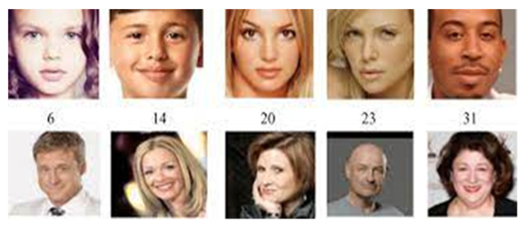
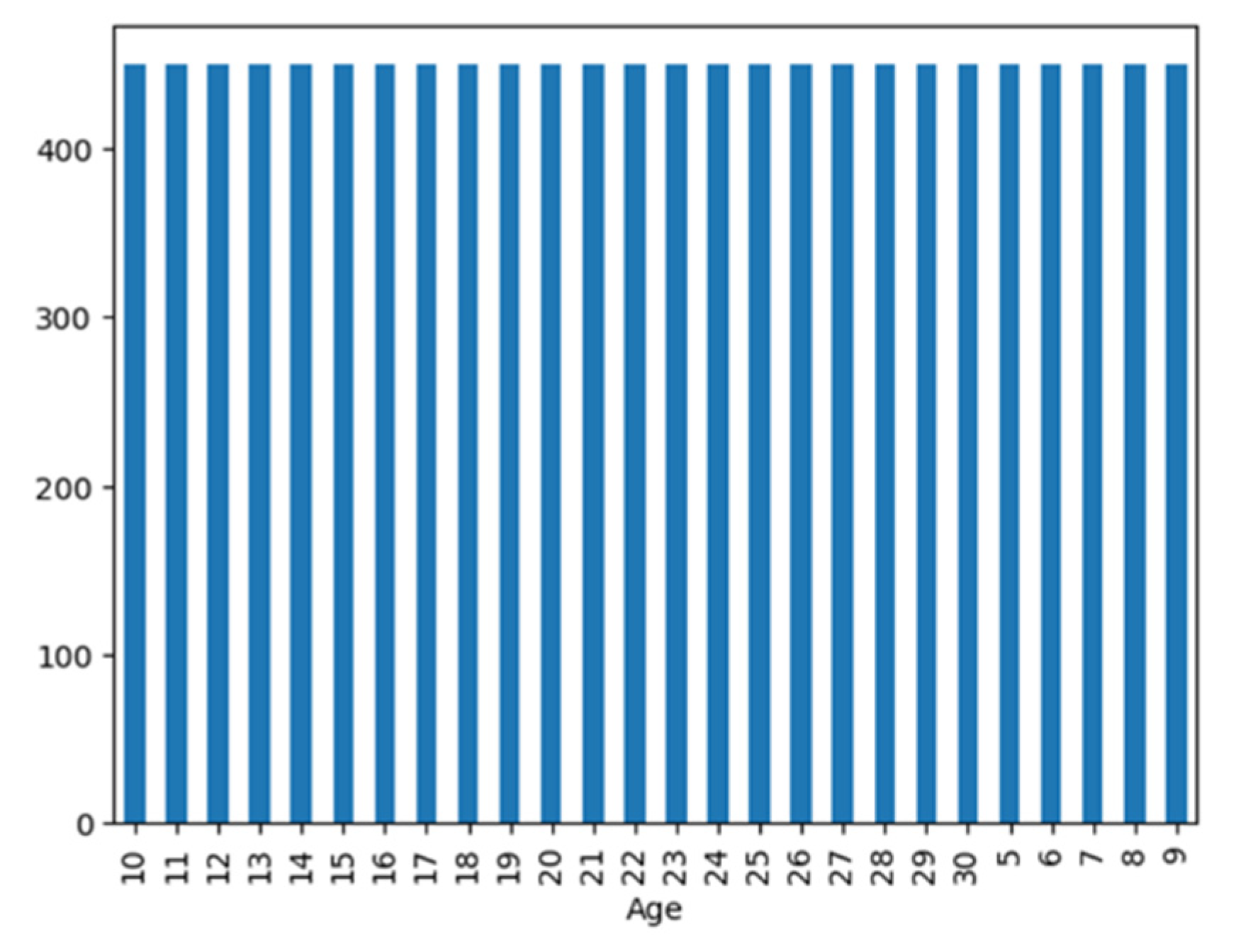
2.1.2. CASIA African facial dataset
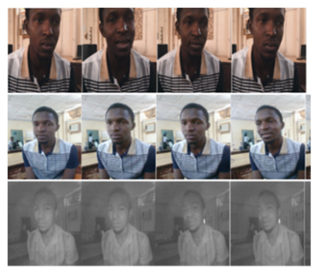
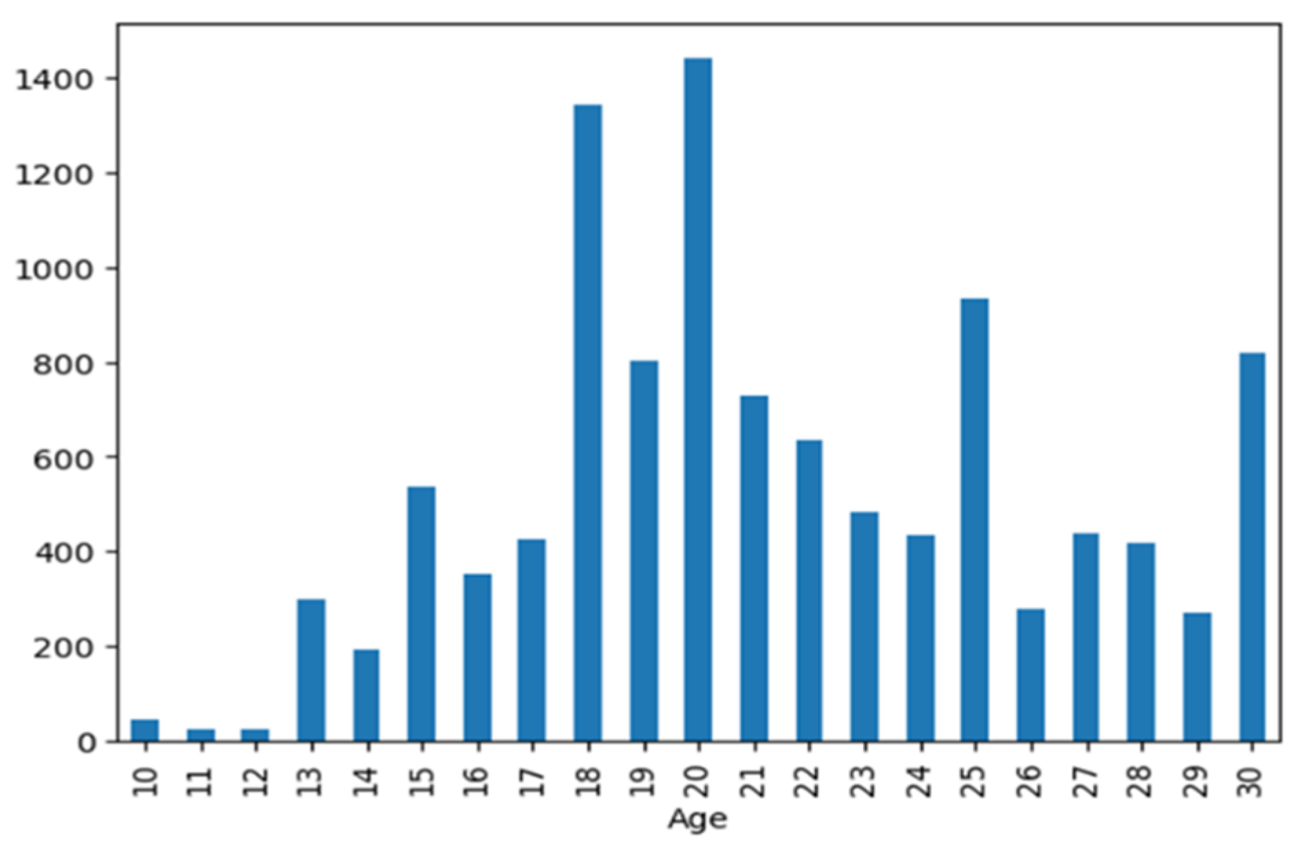
- Training
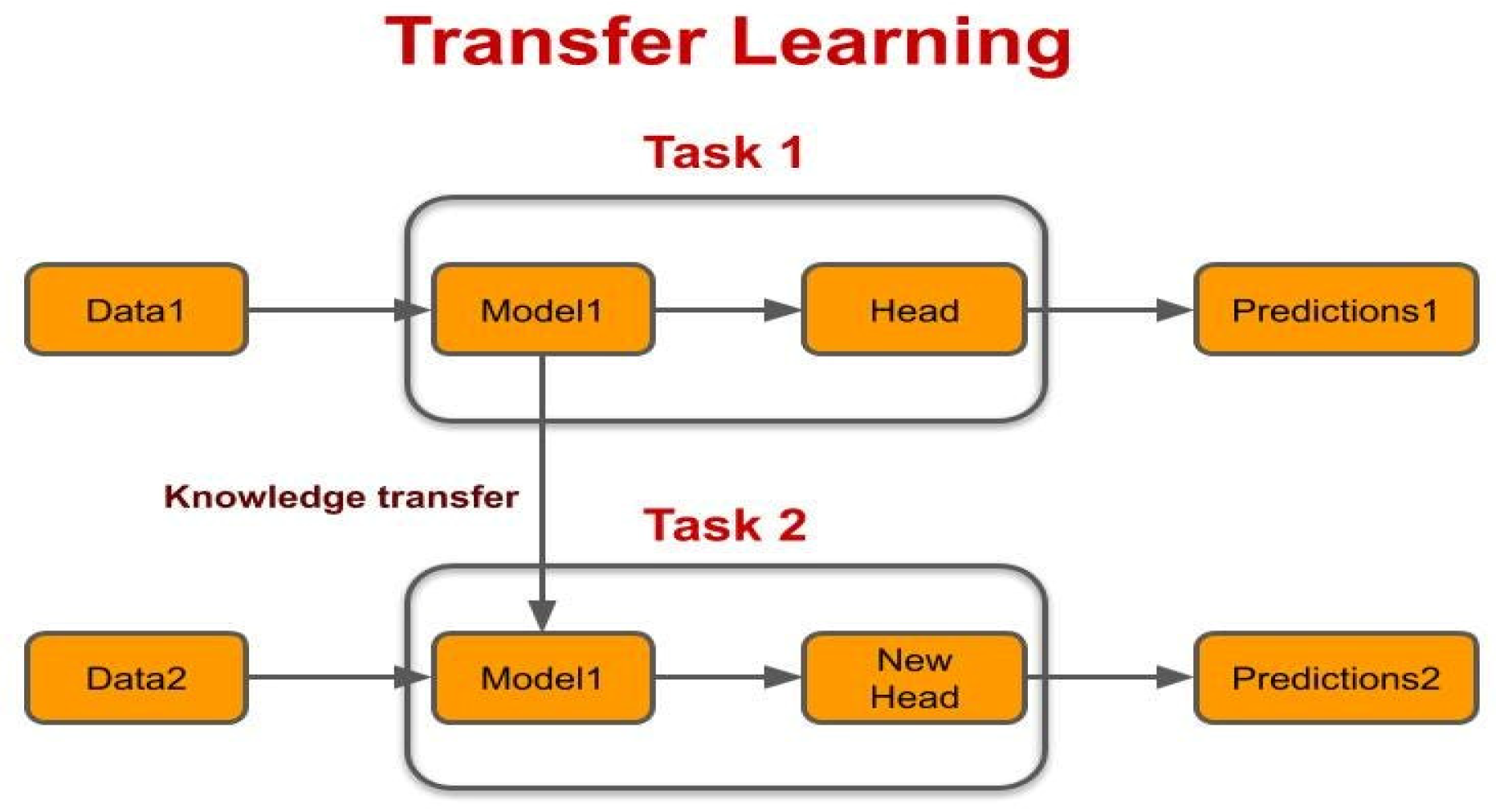
- Transfer Learning Workflow
- Experimental setup
- Training

- Contribution to Knowledge
3. Results
4. Discussion
| Authors | Method | Result | Dataset(s) |
| Akhand et al (2020) | Transfer-Learning | CACD:5-year Grouping (85%). | UTKFace,CACD and FGNet datasets |
| (ResNet 18,ResNet -34,ResNet-50,InceptionNet and Den seNet | 10-Year Grouping (93%) | ||
| Regression | |||
| (MAE of5.17) | |||
| UTK Face:5-year Grouping (97%). | |||
| 10-Year Grouping (99%) | |||
| Regression | |||
| (MAE of 9.19) | |||
| FG-Net:5-year Grouping (100%). | |||
| 10-Year Grouping (100%) | |||
| Regression | |||
| (MAE of 2.64) | |||
| [19] fang et al,(2019) | Trnasfer-Learning VGG 19 | Adience:94% on classification. Regression 1.84 MAE | Adience,CACD |
| CACD: 95% on classification. Regression 5.38 MAE | |||
| [20] Irhebhude et al,(2021) | Principal Component Analysis and support Vector Machine | 10-Year Grouping (95% and 96%)(4 classes) . | Local Dataset and FG-Net |
| [21] Jiang et al (2018) | Caffe DL framwork,CNN | MAE:2.94 | FG-NET and MORPH |
| [22]Ahmed & Viriri (2020) | Transfer-Learning and Bayesian Optimization | MAE) of 1.2 and 2.67 | FERET and FG-NET |
| [23] Ahmed & Viriri (2020) | CNN& Bayesian Optimization | MAE of 2.88 and 1.3 and 3.01 | MORPH, FG-NET and FERET |
| [24] Dagher & Barbara (2021) | transfer learning (pre-trained CNNs, namely VGG, Res-Net, Google-Net, and Alex-Net) | Googlenet (5-year Grouping 74%) | FGNET and the MORPH |
| Googlenet (10-year Grouping 85%) | |||
| Googlenet (15-year Grouping 87%) | |||
| Googlenet (20-year Grouping 89%) | |||
| [25] Ito& Kawai(2018) | transfer learning (AlexNet, VGG16, ResNet152, WideResNet-16-8) single task (STL) learning and multi task learning (MTL) | WRN + STL MAE(7.3) | IMDB |
| WRN+MTL MAE(7.2) | Wide ResidualNe | ||
| [8] | ResNet18 | 2.66 | UTKFace |
| [8] | ResNet34 | 2.64 | FGNet |
| [8] | Inceptionv3 | 5 | Cross-Age-Celebrity-Dataset |
| [8] | DenseNet | 3.19 | UTKFace |
| [8] | ResNet50 | 3.94 | FGNet |
| [9] | GoogleNet | 2.94 | MORPH |
| [9] | GoogleNet | 2.97 | FGNET |
| [10] | CRCNN | 3.74 | MORPH |
| [10] | CRCNN | 4.13 | FGNET |
| [11] | RED+SVM | 6.33 | |
| Our Work | VGG19 | 2.22 | CASIA African Facial Dataset |
| Our work | ResNet 152 | 4.08 | CASIA African Facial Dataset |
| Our work | Mobile Net | 1.10 | CASIA African Facial Dataset |
| Our Work | VGG16 | 1.76 | CASIA African Facial Dataset |
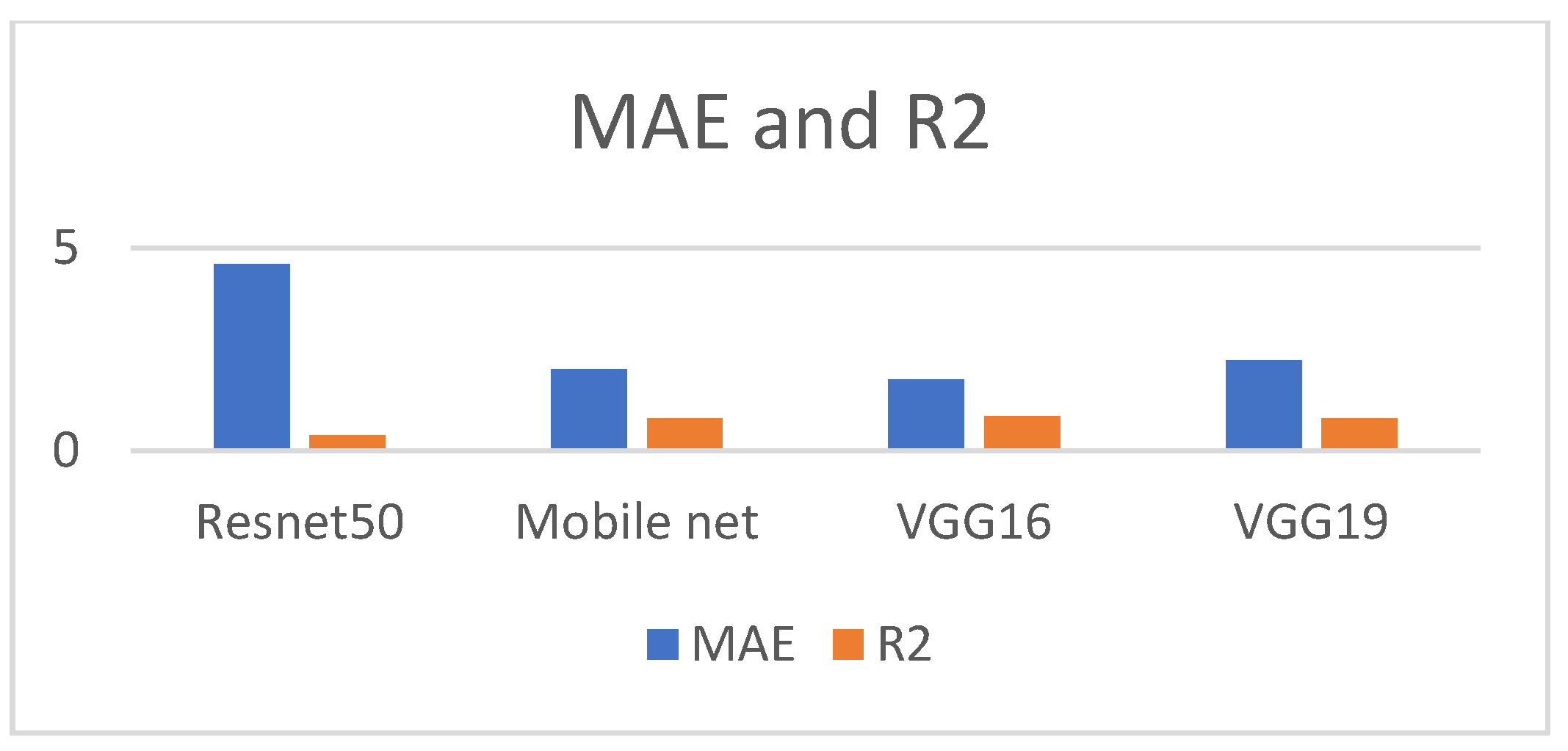
| Our Work | Resnet50 | 4.60 | UTK Facial |
| Our Work | Mobile net | 2.01 | UTK Facial |
| Our Work | VGG16 | 1.75 | UTK Facial |
| Our Work | VGG19 | 2.22 | UTK Facial |
5. Conclusion
Funding
Informed Consent Statement
Data Availability Statement
Conflicts of Interest
References
- C. Alippi, S. Disabato, M. R.-2018 17th Acm/Ieee, And Undefined 2018, “Moving Convolutional Neural Networks To Embedded Systems: The Alexnet And Vgg-16 Case,” Ieeexplore.Ieee.Org, Accessed: May 07, 2023. [Online]. Available: Https://Ieeexplore.Ieee.Org/Abstract/Document/8480072/.
- S. Mascarenhas, M. A.-2021 I. C. On, And Undefined 2021, “A Comparison Between Vgg16, Vgg19 And Resnet50 Architecture Frameworks For Image Classification,” Ieeexplore.Ieee.Org, Accessed: May 07, 2023. [Online]. Available: Https://Ieeexplore.Ieee.Org/Abstract/Document/9687944/.
- D. Theckedath, R. S.-S. C. Science, And Undefined 2020, “Detecting Affect States Using Vgg16, Resnet50 And Se-Resnet50 Networks,” Springer, Accessed: May 07, 2023. [Online]. Available: Https://Link.Springer.Com/Article/10.1007/S42979-020-0114-9.
- A. Singh, N. Rai, P. Sharma, P. Nagrath, And R. Jain, “Age, Gender Prediction And Emotion Recognition Using Convolutional Neural Network.” [Online]. Available: Https://Ssrn.Com/Abstract=3833759.
- Z. A. S Karen, “Very Deep Convolutional Networks For Large-Scale Image Recognition,” Inf Softw Technol, Vol. 51, Pp. 769–784, 2015.
- D. Sinha And M. El-Sharkawy, “Thin Mobilenet: An Enhanced Mobilenet Architecture,” 2019 Ieee 10th Annual Ubiquitous Computing, Electronics And Mobile Communication Conference, Uemcon 2019, Pp. 0280–0285, Oct. 2019. [CrossRef]
- J. Mahadeokar And G. Pesavento, “Open Sourcing A Deep Learning Solution For Detecting Nsfw Images,” Yahoo Engineering, Vol. 24, 2016.
- M. A. H. Akhand, Md. Ijaj Sayim, S. Roy, And N. Siddique, “Human Age Prediction From Facial Image Using Transfer Learning In Deep Convolutional Neural Networks,” Pp. 217–229, 2020. [CrossRef]
- I. Dagher And D. Barbara, “Facial Age Estimation Using Pre-Trained Cnn And Transfer Learning,” Multimed Tools Appl, Vol. 80, No. 13, Pp. 20369–20380, May 2021. [CrossRef]
- F. S. Abousaleh, T. Lim, W. H. Cheng, N. H. Yu, M. A. Hossain, And M. F. Alhamid, “A Novel Comparative Deep Learning Framework For Facial Age Estimation,” Eurasip J Image Video Process, Vol. 2016, No. 1, 2016. [CrossRef]
- K. Y. Chang, C. S. Chen, And Y. P. Hung, “A Ranking Approach For Human Age Estimation Based On Face Images,” In Proceedings - International Conference On Pattern Recognition, 2010. [CrossRef]
- G. George, S. . Adeshina, And M. M. Boukar, “Development Of Android Application For Facial Age Group Classification Using Tensorflow Lite”, Int J Intell Syst Appl Eng, Vol. 11, No. 4, Pp. 11–17, Sep. 2023.
- G. George, S. Adeshina, And M. M. Boukar, “Age Estimation From Facial Images Using Custom Convolutional Neural Network (Cnn)”, Icfar, Vol. 1, Pp. 134–137, Feb. 2023.
- K. Mohammed And G. George, “Identification And Mitigation Of Bias Using Explainable Artificial Intelligence (Xai) For Brain Stroke Prediction”, Ojps, Vol. 4, No. 1, Pp. 19-33, Apr. 2023.
- G. George And C. Uppin, “A Proactive Approach To Network Forensics Intrusion (Denial Of Service Flood Attack) Using Dynamic Features, Selection And Convolution Neural Network”, Ojps, Vol. 2, No. 2, Pp. 01-09, Aug. 2021.
- F. Peter, G. George, K. Mohammed, And U. B. Abubakar, “Evaluation Of Classification Algorithms On Locky Ransomware Using Weka Tool”, Ojps, Vol. 3, No. 2, Pp. 23-34, Sep. 2022.
- Chandrashekhar Uppin, Gilbert George, "Analysis Of Android Malware Using Data Replication Features Extracted By Machine Learning Tools", International Journal Of Scientific Research In Computer Science, Engineering And Information Technology (Ijsrcseit), Issn : 2456-3307, Volume 5, Issue 5, Pp.193-201, September-October-2019. [CrossRef]
- Journal Url : Https://Ijsrcseit.Com/Cseit195532.
- Olufemiajasa, “Alleged Underage Voters: How S’west Lost Voting Strength To N’west,” Vanguard News, Https://Www.Vanguardngr.Com/2023/02/Alleged-Underage-Voters-How-Swest-Lost-Voting-Strength-To-Nwest/ (Accessed Nov. 22, 2023).
- J. Fang, Y. Yuan, X. Lu, and Y. Feng, “Muti-stage learning for gender and age prediction,” Neurocomputing, vol. 334, pp. 114–124, Mar. 2019. [CrossRef]
- M. Irhebhude, A. K.-… C. S. Journal, and undefined 2021, “Northern Nigeria Human Age Estimation From Facial Images Using Rotation Invariant Local Binary Pattern Features with Principal Component Analysis.,” ecsjournal.orgME Irhebhude, AO Kolawole, F AbdullahiEgyptian Computer Science Journal, 2021•ecsjournal.org, Accessed: Aug. 06, 2023. [Online]. Available: http://ecsjournal.org/Archive/Volume45/Issue1/2.pdf.
- F. Jiang, Y. Zhang, and G. Yang, “Facial Age Estimation Method Based on Fusion Classification and Regression Model,” in MATEC Web of Conferences, EDP Sciences, Nov. 2018. [CrossRef]
- M. Ahmed and S. Viriri, “Deep learning using bayesian optimization for facial age estimation,” in Lecture Notes in Computer Science (including subseries Lecture Notes in Artificial Intelligence and Lecture Notes in Bioinformatics), 2019. [CrossRef]
- M. Ahmed and S. Viriri, “Facial Age Estimation using Transfer Learning and Bayesian Optimization based on Gender Information,” Signal Image Process, vol. 11, no. 6, 2020. [CrossRef]
- I. Dagher and D. Barbara, “Facial age estimation using pre-trained CNN and transfer learning,” Multimed Tools Appl, vol. 80, no. 13, pp. 20369–20380, May 2021. [CrossRef]
- K. Ito, H. Kawai, T. Okano, T. A.-2018 A.-P. S. and, and undefined 2018, “Age and gender prediction from face images using convolutional neural network,” ieeexplore.ieee.orgK Ito, H Kawai, T Okano, T Aoki2018 Asia-Pacific Signal and Information Processing Association, 2018•ieeexplore.ieee.org, Accessed: Jul. 22, 2023. [Online]. Available: https://ieeexplore.ieee.org/abstract/document/8659655/.
- J. Muhammad, Y. Wang, C. Wang, K. Zhang and Z. Sun, "CASIA-Face-Africa: A Large-Scale African Face Image Database," in IEEE Transactions on Information Forensics and Security, vol. 16, pp. 3634-3646, 2021. [CrossRef]

| Method | MAE | R2 | Dataset |
|---|---|---|---|
| Resnet50 | 4.60 | 0.38 | UTK |
| Mobile net | 2.01 | 0.80 | UTK |
| VGG16 | 1.75 | 0.85 | UTK |
| VGG19 | 2.22 | 0.80 | UTK |
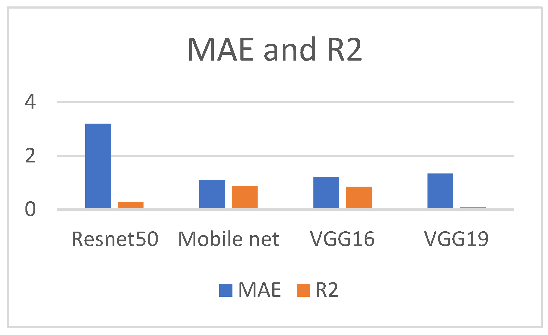
| VGG19 | 1.34 | 0.19 | CASIA |
| ResNet 50 | 3.19 | 0.28 | CASIA |
| Mobile Net | 1.10 | 0.88 | CASIA |
| VGG16 | 1.21 | 0.85 | CASIA |
Disclaimer/Publisher’s Note: The statements, opinions and data contained in all publications are solely those of the individual author(s) and contributor(s) and not of MDPI and/or the editor(s). MDPI and/or the editor(s) disclaim responsibility for any injury to people or property resulting from any ideas, methods, instructions or products referred to in the content. |
© 2024 by the authors. Licensee MDPI, Basel, Switzerland. This article is an open access article distributed under the terms and conditions of the Creative Commons Attribution (CC BY) license (http://creativecommons.org/licenses/by/4.0/).


