Submitted:
30 December 2023
Posted:
03 January 2024
You are already at the latest version
Abstract
Tuning tensor program generation involves navigating a vast search space to find optimal program transformations and measurements for a program on target hardware. The complexity of this process is further amplified by the exponential combinations of transformations, especially in heterogeneous environments. This research addresses these challenges by introducing a novel approach that learns the joint neural network and hardware features space, facilitating knowledge transfer to new, unseen target hardware. A comprehensive analysis is conducted on the existing state-of-the-art dataset, TenSet, including a thorough examination of test split strategies and the proposal of methodologies for dataset pruning. Leveraging an attention-inspired technique, we tailor the tuning of tensor programs to embed both neural network and hardware-specific features. Notably, our approach substantially reduces the dataset size by up to 53% compared to the baseline without compromising Pairwise Comparison Accuracy (PCA). Furthermore, our proposed methodology demonstrates competitive or improved mean inference times with only 25%40% of the baseline tuning time across various networks and target hardware. The attention-based tuner can effectively utilize schedules learned from previous hardware program measurements to optimize tensor program tuning on previously unseen hardware, achieving a top-5 accuracy exceeding 90%. This research introduces a significant advancement in auto-tuning tensor program generation, addressing the complexities associated with heterogeneous environments and showcasing promising results regarding efficiency and accuracy.
Keywords:
auto-tuning
; deep learning compilers
; heterogeneous transfer learning
; tensor program generation
1. Introduction
Deep neural networks (DNN) are crucial in various artificial intelligence domains, impacting industries and scientific fields. The development of DNNs has been propelled by advancements in computing hardware and specialized accelerators, enabling the efficient execution of tensor programs through hand-tuned deep-learning libraries. However, these libraries often need more scalability. Tensor compilers like XLA [1], TVM [2], and Glow [3] and TACO [4] facilitate optimizations for input computation graphs [5], offering both hardware-independent (high-level) and dependent (low-level) optimizations.
A tensor compiler analyzes computation graphs and optimizes mathematical expressions for efficient tensor programs. The evolution of deep neural architectures, from simple to complex models like Megatron-Turing Natural Language Generation (MT-NLG) [6], has led to a vast search space for compiler optimizations. Despite automatic tuning of tensor compilers becoming prevalent, data-driven approaches face challenges due to resource-intensive methodologies and the need for significant hardware data.
Advancements in hardware, including GPUs and domain-specific accelerators, along with popular DL frameworks like TensorFlow [7] and PyTorch [8], provide optimized kernel support for driving innovations in deep learning. The evolving landscape of DNN architectures and backend hardware has significantly expanded the search space for compiler optimizations. This extensive space, encompassing optimizations like tiling and vectorization, poses challenges for data-driven approaches in auto-tuning tensor compilers to generate efficient tensor programs. As automatic tuning of tensor compilers gains prevalence, methodologies based on data-driven cost modeling and intelligent techniques necessitate substantial hardware data for effective model learning. However, these datasets are often experiment-specific in the HPC domain, and resource-intensive techniques face obstacles when introducing new hardware due to the need to retrain the cost model or tuner from scratch.
Moreover, a majority of these cost models [9,10] rely on training and testing data derived from identical probability distributions, with the assumption that the source and target compute hardware are the same. Yet, in the era of diverse and heterogeneous hardware systems encompassing various generations of CPUs and GPUs, such an assumption may prove impractical. For example, a tuner trained to optimize tensor programs for a specific vendor’s CPU in a deep learning workload may not be as effective in generating efficient tensor programs for a CPU from a different vendor. To address this challenge, transfer learning has proven beneficial by assimilating context from neural network tasks and applying it to novel contexts.
Thus, the imperative for a transfer learning-based approach, demanding less data and swift adaptability to new hardware, becomes evident. Cost models trained on restricted hardware or specific neural network tasks often lack transfer learning capabilities. Consequently, it proves efficient to map the heterogeneous feature space across devices and fine-tune only the necessary features rather than undergoing a complete retraining process. In situations where manually tuned libraries struggle to offer optimized support for new hardware and operators, auto-tuners, with their capacity to learn from limited data, can significantly reduce tuning time and the duration needed for online device measurement by concentrating on acquiring knowledge about high-performance kernels. Recent studies have introduced transfer learning methods specifically for the same source and target hardware [10,11,12]. We advocate for heterogeneous transfer learning by mapping the kernel as a feature space in a new context.
This paper builds upon the research conducted by Verma et al. [13] and scrutinizes the contemporary methods employed for generating tensor programs through transfer learning, specifically targeting CPU and GPU-based systems. Leveraging probabilistic and exploratory analyses, we strive to attain comparable results using a reduced dataset compared to the baseline, employing various split strategies. Our proposed approach centers on transfer learning to produce efficient tensor programs, aiming for minimized tuning time and a decreased number of kernel measurements across diverse hardware platforms. The significant contributions of this paper are as follows:
- Conducted a thorough examination of existing research to extract and assimilate insights from the combined neural network and hardware features.
- Formulated a proposed methodology grounded in the principles of minimizing kernel measurements and leveraging efficient transfer learning.
- Implemented an optimized tuner based on the aforementioned key points and showcased results for heterogeneous transfer learning. The outcomes demonstrated comparable or improved mean inference time, accompanied by a noteworthy 3x-5x reduction in tuning time and up to a 53% reduction in dataset size.
The remainder of the paper is organized as follows: Section 2 gives the requisite background to understand the problem and presents the related work in this area. Section 3 describes the proposed methodology used in the study. Section 4 and Section 5 discuss experimentation and results, respectively. Section 6 provides a conclusion and potential future steps.
2. Background and Related Work
Autotuning of tensor programs poses a significant challenge due to the time-consuming nature of the auto-scheduling process. Tuning can take several hours for a DNN model, depending on factors such as program complexity and available hardware resources. This extended tuning duration becomes a hurdle for timely deployment, as achieving the best inference times requires thoroughly exploring the schedule space. Methods to shorten the search process, like restricting the tuner’s operation time or focusing on tuning a part of the model’s kernels, come with trade-offs. Users need to consider the balance between potential improvements in performance and the reduction in tuning time. The primary challenge in tensor program autotuning is the time-intensive measurement of tensor program latency. This process involves multiple steps, network transfers, compilation complexities, and the need for repetitive measurements to ensure accuracy. These challenges highlight the complexity of autotuning tensor programs. In this section, we discuss previous work on improving the effectiveness and efficiency of tuning tensor programs, specifically addressing the requirements of datasets and tuning time.
2.1. Cross-device Learning
The search space in cross-device learning is vast, spanning from orders of millions (CPU) to billions (GPU), resulting in a considerable search space and associated high costs in terms of search time. Transferring knowledge from auto-scheduled pre-tuned kernels to untuned kernels holds significant promise in addressing these challenges. As discussed in the literature, various solutions have been proposed to tackle different aspects of transfer learning [12]. Gibson [12] and Verma et al.[14] have classified tasks into classes to enhance optimization selection. Mendis et al.[15] employ a hierarchical LSTM-based approach, predicting throughput based on the opcodes and operands of instructions in a basic block. Their proposed solution demonstrates portability across various processor micro-architectures. In another study [16], a cost model query optimizer is utilized to enhance resource utilization and reduce operational costs. Zheng et al. [17] introduce an end-to-end pipeline to optimize synchronization strategies based on model structures and resource specifications, thereby simplifying data-parallel distributed machine learning across devices. In our work, we propose an efficient dataset pruning technique to learn joint kernel and hardware features. This approach facilitates streamlined tuning by focusing on prominent kernels, contributing to enhanced efficiency in the learning process.
Gibson et al. [12] introduce a novel approach to reuse auto-scheduling strategies among tensor programs efficiently. Specifically, they explore collections of auto-scheduling strategies derived from previously optimized deep neural networks (DNNs) and leverage them to enhance the inference efficiency of a new DNN. A comparative evaluation is conducted, contrasting the efficacy of the proposed approach with the state-of-the-art auto-scheduling framework known as Ansor. The proposed method capitalizes on the inherent similarities found within kernels that encompass identical operations but exhibit diverse data sizes. This similarity enables the seamless reuse of scheduling strategies across different tensor programs, resulting in a notable reduction in both time and computational expenses associated with the optimization process. Notably, this investigation focuses exclusively on the CPU platform and does not encompass hardware-specific characterizations when selecting heuristics for transfer tuning. Furthermore, the authors limit their selection of kernels to those derived from networks within the same architectural class, omitting the consideration of potential knowledge transfer between networks of distinct architectures or hardware configurations.
In a multi-task approach [18], the authors introduce a novel approach to cost modeling for auto-tuning tensor program generation using multi-task learning. This approach involves extracting features from schedule primitives obtained through offline measurements. By doing so, the model gains valuable insights from a wide range of hardware and network configurations. Additionally, the authors employ NLP regression techniques to facilitate the automation of scheduling decisions. To address the complexity of the problem, they structure it as a multi-task learning framework. Each task corresponds to a specific hardware platform for a given tensor program. This innovative approach allows for improved performance even with a limited dataset. In contrast, our approach builds on top of their approach. We employ probabilistic sampling techniques to curate the dataset, jointly focusing on the FLOPs and execution time of the kernels. During the fine-tuning process, we prioritize tasks with high significance, guided by prior measurements. This strategy sets our approach apart from the one presented by the authors, providing a unique and effective method for tackling the auto-tuning challenge.
Further, there are approaches [19] employing model distillation as a technique for segregating both transferable and non-transferable parameters. The authors introduce a novel design inspired by the lottery ticket hypothesis, pinpointing features that can seamlessly transfer across different hardware configurations via domain adaptation. It is worth noting that this work stands among the pioneering efforts in harnessing transfer learning for such purposes. The proposed approach can automatically discern the transferable, hardware-agnostic parameters of a pre-trained cost model. It accomplishes this feat through cross-device cost model adaptation, achieved via fine-tuning, and does so within a notably abbreviated search time for a new device. Notably, this approach facilitates cross-device domain adaptation for a trained cost model by updating the domain-invariant parameters during online learning. This innovation carries significant implications, particularly in enhancing the efficiency of the auto-tuning process and elevating the end-to-end throughput of tuned tensor programs on the target device. As with any approach, there are certain limitations to consider. In this case, the method does not address knowledge transfer from cross-subgraph tensor optimization. Nevertheless, the authors acknowledge this as an area for future exploration and development.
2.2. Machine Learning-based Auto Tuners
Machine learning approaches for optimizing tensor programs [9,20,21] are heavily researched for tensor compilers and deep learning workloads by Verma et al. [22]. The work from Zheng et al. [23] generates tensor programs for DL workloads by exploring optimization combinations through a hierarchical search space and optimizing sub-graphs with a task scheduler. The use of LSTM to sequence optimization choices [24] has been explored. Moreover, Whaley et al. [25] automate generating and optimizing numerical software for processors with deep memory hierarchies and pipelined functional units, making it adaptable across server and mobile platforms.
Additionally, authors have employed reinforcement learning (RL) in various works. Mendis et al. [26] investigate transforming the integer linear programming solver into a graph neural network-based policy for auto-generating vectorization schemes. Also, domain-specific compilers such as COMET [27], JAX [28], and NWChem [29] are under active research for optimizing program execution. Lately, Ryu et al. [10] have proposed a one-shot tuner for the tensor compilers. Its limitation is that it considers only task-specific information, which prevents it from being applied for transfer learning. On the other hand, we employ neural network and hardware platform information so that the auto-tuner can learn better.
Bi et al. [30] introduce a novel approach to tensor program optimization, explicitly focusing on biased-diversity-based Active Learning. The primary objective is to streamline the training process while maintaining a consistent program performance optimization level comparable to the baseline Tenset. They implement a unique biased-diversity-based diversity scheme within their framework to achieve this. This scheme addresses a critical issue in active learning: the problem of overestimation when utilizing brute-force sampling techniques. The framework comprises two components: AL-based model pre-training and pre-trained-model-based program optimization. However, it is essential to note that this framework employs random program sampling without considering hardware characterization. Subsequently, these sampled programs are executed on the hardware to collect performance measurements. To generate unlabeled program datasets, the framework randomly samples transformed tensor programs from predefined optimization tasks. The authors employ a diversity-based selection approach to balance the distribution of these samples and, in particular, increase the proportion of high-performance programs. This strategy is designed to enhance the diversity of selected programs’ performance, ultimately contributing to the effectiveness of the active learning process.
In another research, Liu et al. [31] address the challenge of latency estimation using evolving relational databases. To achieve this, they introduce two integral components: the Neural Network Latency Query System (NNLQ) and the Neural Network Latency Prediction System (NNLP). The central innovation of this system lies in its capacity to automatically convert deep neural networks (DNNs) into executable formats based on prior knowledge derived from offline latency measurements. The Latency Querying System employs a Graph Neural Network (GNN)-based foundation to extract cohesive graph embeddings for various DNN models. It also incorporates a multi-headed approach to facilitate concurrent latency prediction across multiple hardware platforms. This framework further empowers users to discern the supported tensor operators on a given hardware setup while considering achievable latency and the trade-off between latency and accuracy. However, it is essential to note that the proposed system primarily functions as a querying tool and does not extend to providing fine-grained control over scheduling processes to optimize either latency or accuracy. Consequently, the influence of auto-scheduling remains outside the scope of its functionality.
2.3. Hardware-aware Auto Tuners
In addition to the works mentioned earlier, we examined specific studies to understand them better, as explained below.
The current state-of-the-art deep learning compilers undertake optimizations in a two-step fashion, involving high-level graph optimizations followed by operator-level optimizations. In this study [32], researchers shift their focus towards a unified optimization approach. They introduce a framework that incorporates a versatile transformation module designed to enhance the layouts and loops through fundamental functions. Additionally, this framework incorporates an auto-tuning module to facilitate these optimizations. To address the overhead associated with layout transformations, they propose a mechanism known as layout propagation. Under this mechanism, the upstream operator assumes responsibility for accommodating varying input layouts. In cases of operator fusion, it extends these new layouts downstream throughout the computation graph. This propagation mechanism manages the reconstruction of loops and aligns the loop nests of multiple operators for fusion with minimal additional computational cost. Furthermore, they tackle the challenge of search space reconstruction in the auto-tuning process by dividing it into two distinct stages: joint and loop-only stages. During the joint stage, the system explores optimal tensor layouts, while the loop-only stage exclusively focuses on fine-tuning loops while maintaining the previously determined layouts. To streamline the search space exploration, they employ effective pruning strategies. First, they restrict the creation of layout transformation spaces to tensors accessed by complex operators. Second, they identify a promising subspace by tailoring a tuning template for each tensor accessed by complex operators. These templates are constructed based on a comprehensive analysis of layout optimization, considering both operator and hardware characteristics. It’s worth noting that this template-based approach aims to address scalability concerns associated with manually created templates, similar to the challenges faced by the auto-tvm approach.
On the other hand, Ahn et al. [33] focus on the mathematical representation of GPUs’ hardware specifications, a fundamental aspect of the study. The approach here embraces a strategy rooted in hardware awareness, bringing forth an intelligent and strategic exploration and sampling process. This method is carefully designed to guide the search algorithm towards regions within the search space with a higher potential for improving performance outcomes. The initial step entails the generation of prior probability distributions that encapsulate various dimensions within the expansive search space. These distributions subsequently become invaluable inputs to the Bayesian optimization framework, enhancing its decision-making capabilities. Moreover, a vital element of this work is integrating a lightweight neural function that is pivotal in striking the delicate balance between exploration and exploitation—a fundamental challenge in optimization tasks. The authors’ innovation extends to applying the Meta-Optimizer, a powerful tool that orchestrates achieving an optimal equilibrium between exploration and exploitation. This blend of techniques seamlessly incorporates hardware awareness into the Hardware-Aware Exploration module, culminating in an approach that demonstrates a keen understanding of GPU hardware characteristics while optimizing the search process.
Taking a different approach, Li et al. [34] have proposed an auto-tuning framework that generates tensor programs by exploiting the subgraph similarities. The framework introduces a novel approach by harnessing subgraph similarities and systematically organizing them into subgraph families. Within this context, a significant enhancement is achieved through the development of cost models built on a per-family basis, improving the precision in estimating high-potential program candidates. This advancement contributes significantly to the overall optimization of tensor program generation. A notable achievement of this framework is its ability to reduce the number of program candidates subjected to resource-intensive hardware measurements. This is accomplished by utilizing highly accurate cost models on a family basis, without compromising the quality of the search. Furthermore, the literature survey highlights the authors’ in-depth analysis of the accuracy of these cost models regarding various subgraph attributes, including the number of operators, core operators, and operator sequences. The findings presented in this study shed light on the framework’s effectiveness and its potential impact on optimizing tensor program generation, making it a valuable contribution to the field of automated program tuning.
Lastly, Mu et al. [35] introduce a specialized auto-tuner for deep learning operators that adapts to hardware, particularly tailored for tensors with dynamic shapes. They use micro-kernels akin to DietCode, optimized explicitly for dynamic shape tensors. While DietCode primarily focuses on tensor shapes, HAOTuner goes further by considering the available hardware resources. They present an algorithm for selecting hardware-friendly micro-kernels, reducing the time required for tuning. Additionally, they offer a model transfer solution that enables the rapid deployment of the cost model on diverse hardware platforms. The evaluation of HAOTuner covers six different GPU types. However, it’s important to note that their proposed method is constrained by hardware architecture compatibility, as it exclusively functions with CUDA-enabled hardware. This limitation restricts its applicability for transfer learning across various hardware architectures.
3. Design And Implementation
In this section, we present our methodology as follows: Section 3.1 offers a comprehensive overview of the entire flow and individual components, Section 3.2 delves into the proposed optimizations and opportunities for efficient heterogeneous transfer learning with a reduced dataset, and Section 3.3 details the adaptive auto-tuner architecture.
3.1. End-to-End Execution Steps of the Framework
Figure 1 presents a comprehensive overview of our framework’s end-to-end workflow. Our approach is based on TVM v0.8dev0, serving as the foundational platform for conducting heterogeneous transfer learning. The framework is designed to facilitate the seamless transition of computational models between different hardware environments. In this process, the user interacts with the framework through the TVM APIs, engaging in a series of key steps, as illustrated by the circled numbers:
- The user initiates the workflow by providing the computational framework in a supported format, such as TensorFlow, ONNX [36], or PyTorch.
- The framework undertakes high-level optimization and subgraph partitioning, resulting in the generation of smaller subgraphs. These subgraphs constitute the candidates for the search space for subsequent feature extraction operations. Measurements are performed on these subgraphs for a particular hardware configuration. The outcomes are subsequently stored in individual JSON [37] files for each subgraph, encompassing schedule primitive hints and the execution time for each auto-generated tensor program.
- Domain-specific information, encompassing details like kernel dimensions and tensor operations, is preserved from the subgraphs, forming a distinctive feature set.
- For each data-point entry or kernel, critical hardware information is meticulously recorded, including hardware architecture, maximum thread count, register allocation, and threads per block. This data constitutes the static hardware dataset.
- A probabilistic and exploratory study is conducted on this feature set to identify features of significant importance. This hardware characterization plays a pivotal role in mapping features from the source hardware to the target hardware, ensuring compatibility. The auto-tuner is trained using this dataset, extending the principles of a one-shot tuner [10]. This training equips the auto-tuner with the capability to generate tensor programs on the target device automatically, with or without retraining.
- For users seeking fine-tuning capabilities, the framework offers the option to fine-tune the auto-tuner using online hardware features. Experimental work includes selective task retraining and a methodology inspired by the Lottery Ticket Hypothesis-based technique [19]. Our approach reduces retraining time and minimizes the dataset size required for fine-tuning. The utilization of attention heads supports memory-augmented fine-tuning through bidirectional LSTM [38]. Given the framework’s attention-based training strategy, the auto-tuner model undergoes a comprehensive training phase only once, mitigating the necessity for extensive data on the target device for full retraining.
- Following the execution of steps 5 and 6, a set of top-k tensor programs is generated. To facilitate user selection based on specified metrics, we employ ranking loss. This ensures that users have the flexibility to choose a tensor program from the top-k list according to their preferences and the defined metric.
- Finally, the proposed tensor programs are deployed on the target hardware, and their performance is rigorously evaluated.
This end-to-end workflow represents a systematic and efficient approach to enabling the seamless transfer of computational models across different hardware environments. The framework’s ability to adapt and fine-tune for specific hardware configurations offers enhanced flexibility and performance optimization.
In our study, we utilized the TenSet dataset [11] as the foundation for our baseline measurements. According to the assertions made by the dataset’s authors, it is positioned as a resource suitable for generating tensor programs through the application of transfer learning. The dataset’s strength lies in its diversity, fostering generalization, and encompassing performance data points across multiple platforms, including CPUs from Intel and ARM, and NVIDIA GPUs. Section 3.3 delves into the discussion of how these foundational characteristics make the dataset conducive for effective transfer learning using the proposed auto-tuner. Further details about the dataset can be found in [11]. For a concise overview of the hardware platforms and their associated characteristics considered in our investigation, refer to Table 1.
3.2. Hardware-Aware Kernel Sampling
We conducted an extensive and experimental analysis of the TenSet dataset to gain insights into the neural network and hardware features influencing metrics such as flops, throughput, and latency. The dataset comprises over 13,000 tasks derived from 120 networks, measured on six distinct hardware platforms. These measurements include throughput and latency, considering various neural network and hardware parameters, resulting in a dataset encompassing over 52 million measurements. In our analysis (as detailed in Table 1), we focused on the first four platforms to understand tasks, the applied schedules, associated performance, and hardware parameters. The latter half of the hardware serves for evaluating and establishing the viability of cross-device or transfer learning.
In addition to neural network details such as tensor operations and input/output shapes, hardware parameters (as presented in Table 2) are also considered. While we specifically present hardware features for CPU and GPU, the approach can be extended to other heterogeneous devices. Through dataset analysis, we observed that high-performing kernels often correlate with specific hardware parameters. Employing probabilistic sampling helps mitigate biased kernel selection, preventing the inclusion of kernels that might lead to lower FLOPs or result in invalid computation graphs. We rigorously filtered out measurements and kernels deemed invalid or low-performing. Notably, our observations underscore the impact of large search spaces, selected via random sampling of kernels, causing performance regression in existing cost modeling practices.
In our efforts to streamline the tensor program generation, we strategically pruned the expansive search space. Relying on a search task driven by measurements from randomly sampled kernels proves unreliable, particularly when the search space lacks richness. Our observations underscore that certain hardware parameters, such as the number of cores, exhibit less significance as features compared to flop count, especially in relation to latency. This arises from the necessity for diverse kernel combinations and hardware features within the dataset under consideration.
Consequently, we conducted an evaluation focusing on the interplay of FLOPs count, kernel shape, and execution time for various tensor operations on a specific hardware platform. The outcomes, detailed in Table 3, reveal similar behavior between CPUs and GPUs in selecting optimal kernel shapes. However, a notable discrepancy in execution time emerges based on the compute hardware. In response, we strategically sampled kernels by jointly exploring tensor operations, kernel shapes, and hardware parameters, prioritizing FLOPs count and execution time. The initial set of kernels, extracted from six diverse neural networks to encompass prominent classes, is a dynamic list that continues to evolve. We are actively developing an intelligent algorithm to efficiently accommodate new network classes as they are introduced. Our experimentation, employing metrics such as rmse, equation 1, and ranking loss, equation 2, has led us to favor rmse for performance evaluation in our tuner. Notably, the analysis of the costs associated with the selected kernels’ measurement records reveals the presence of local minima. To circumvent this, we used simulated annealing within TVM. However, the computational intensity of this approach results in a significant time investment to identify global optima. Addressing this, we have identified optimization opportunities for future work.
where:
where:
3.3. Auto-tuner Architecture
We have employed an attention-based [39] tuner to experiment with a joint neural network and hardware features as part of the task. In addressing the generation of tensor programs with reduced latency, it is crucial to recognize the convex nature of the problem, rendering search-based methodologies particularly useful. Leveraging schedule information from the comprehensive TenSet dataset, we focused on feature extraction, with the length of the schedule primitive serving as the designated sequence length. The internally processed features are subsequently encoded using the one-hot encoding technique, facilitating their integration into the embedding layer and determining the overall embedding size. As highlighted earlier in the discourse, our analysis targeted the identification of high-performing tensor kernels. Notably, our findings reveal a prevalence of these high-performing kernel tensor program schedules across both CPU and GPU architectures, underscoring their cross-platform efficacy.
In outlining our model architecture, we employ an attention mechanism (equation 3) as the core component to grasp contextual features. This mechanism operates simultaneously, allowing for efficient parallel execution. Our model undergoes training using the existing dataset, and in the event of encountering new hardware, we fine-tune the learned auto-tuner to adapt to the updated conditions by learning new weights. To facilitate transfer learning and accommodate updates through fine-tuning, we incorporate multiple heads (equation 4), each tailored to the specific hardware parameters obtained from the system under test. This approach enhances the adaptability and performance of our model across diverse hardware configurations.
where:
where:
We designed our auto-tuner for efficient attention-based processing with applications in multiple tasks. The architecture incorporates a sequential encoder, composed of four linear layers with ReLU activation functions, to capture and transform input features. An attention mechanism is employed, allowing for parallel execution and facilitating the extraction of contextual information. The attention output is enhanced through residual connections in a series of residual blocks, each containing two linear layers followed by ReLU activation and batch normalization. This design choice aims to mitigate vanishing gradient issues and enhance training stability. The model further incorporates multiple heads, each tailored to specific hardware parameters, through which transfer learning and fine-tuning are facilitated. Notably, additional layers, including linear transformations and batch normalization, are introduced in the heads to increase model depth and expressiveness. This augmented depth, along with the inclusion of batch normalization, contributes to improved convergence during training. Overall, the model is structured to adapt effectively to varying hardware configurations, leverage attention mechanisms for contextual understanding, and harness the benefits of both residual connections and batch normalization for enhanced performance in multitask learning scenarios.
The training methodology encompasses the optimization process for the proposed auto-tuner, leveraging an attention-based architecture. The model is initialized with tailored configurations featuring four hidden layers, and parallelized training is achieved through the application of torch.nn.DataParallel. The chosen optimizer is Adam, complemented by an associated learning rate scheduling strategy. After testing multiple configurations, we chose the near-optimal values based on empirical evaluation, including a batch size of 16, 200 epochs, and other hyperparameters listed in Table 4.
4. Evaluation
4.1. Experimental Setup
Platform: Our study experiment used heterogeneous architectures like Nvidia GPUs- H100, A100, A40, ARM A64FX, and Intel Xeon CPU. We chose different generations of GPUs and CPUs to study the impact of architectural differences. We chose different generations of GPUs and CPUs to study the effects of architectural differences.
Dataset and Model: This study employs TVM v0.8dev0 and PyTorch v0.7.1 for its implementations. As baseline tuners, we utilized XGBoost (XGB) [40], multi-layer perception (MLP) [41], and LightGBM (LGBM) [42]. Our proposed tuner introduces an attention-based multi-head model, as elaborated in Section 3.3. The baseline TenSet dataset [11] utilized in this study comprises over 51 million measurement records. These records pertain to 2,308 subgraphs extracted from 120 networks. The baseline dataset for each subgraph contains measurements on various hardware, as delineated in Table 1.
Baseline Measurements: For the baseline, we used the TenSet dataset, commit 35774ed. Based on the previous work [11], we have considered 800 tasks with 400 measurements as the baseline. We used Platinum-8272 for the CPU dataset and Nvidia Tesla T4 for the GPU dataset. Further, we took record measurements on A64FX and H100 for the auto-tuner’s extensive feature analysis and evaluation.
4.2. Dataset Sampling
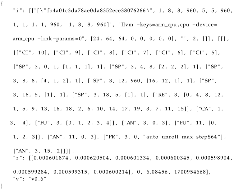
A measurement record corresponding to a task in the dataset is encapsulated within JSON files, delineating three crucial components: first, the input information and the schedules generated (i); second, the measured performance across multiple runs (r); and finally, the version information (v). The concrete manifestation of such a measured record for a randomly chosen task is depicted in Listing 1. This exemplar showcases an intricate array of details, including explicit hardware specifications such as "llvm-keys =arm_cpu, cpu-device=arm_cpu-link-params=0", intricate tensor information, and the automatically generated scheduling primitives (e.g., CI, SP, etc.) along with their respective parameters. To rectify erroneous measurements, we incorporate warm runs for each measurement and meticulously exclude any configurations deemed invalid. In Table 5, a comprehensive list of scheduling primitives, derived from measurements conducted on hardware utilizing TVM, is presented. Each abbreviation corresponds to a specific scheduling step, offering a succinct representation of the intricacies involved in the optimization process. These primitives encapsulate a range of tasks, from annotation (AN) and fusing (FU) steps to pragma (PR) application and reordering (RE) procedures. Notably, the table encompasses more intricate steps such as storage alignment (SA), compute at (CA), and compute in-line (CI) steps, highlighting the nuanced nature of the optimization strategies employed. Additionally, the inclusion of cache-related steps such as cache read (CHR) and cache write (CHW) underscores the importance of memory considerations in optimizing performance. A schedule constitutes a compilation of computational transformations, often referred to as schedule primitives, that are applied to the loops within a program, thereby modifying the sequence of computations. Diverse schedules contribute to varying degrees of locality and performance for tensor programs. Consequently, it becomes imperative to delve into the search space and autonomously generate optimized schedules to enhance overall efficiency.
| Listing 1: A Sample Measured Record On A64FX |
 |
We conducted a comprehensive exploration of hardware measurements, extending our analysis to encompass two additional hardware platforms: NVIDIA’s H100 and ARM A64FX. This endeavor aimed to unravel valuable insights from the recorded data, subsequently employed as embeddings in our attention-based auto-tuner. The cumulative count of measurements amassed across both hardware platforms reached an impressive total of 9,232,000.
On the H100 hardware, the automatically generated schedule sequence lengths exhibited a diverse spectrum, spanning from 5 to 69. Conversely, within the measured records on the A64FX platform, the sequence lengths manifested a range between 3 and 54. Noteworthy variations in the occurrences of schedule primitives within a measured record were observed, and these intricacies are meticulously documented in the accompanying Table 6. In this context, "sequence length" refers to the total length of the schedule primitives when encoded as a string, as illustrated below. The term "total occurrence" denotes the overall presence of such encoded strings across all 2308 sub-graphs. For each individual subgraph, a comprehensive set of 4000 measurements were systematically conducted.
To illustrate, an example sequence with a length of 5 may take the form of FU_SP_AN_AN_PR or CA_CA_FU_AN_PR, complete with parameter values tailored to the specific kernel. This exemplar serves as a glimpse into the rich diversity found in the measured records. Based on these insightful analyses, we have made informed decisions regarding the embedding strategies employed by our auto-tuner, ensuring a robust and nuanced approach.
As detailed in Section 3.2, we have conducted sampling on the dataset. Utilizing data sampling techniques that prioritize the importance of features, particularly in relation to FLOPs count, enabled a reduction of 43% in the GPU dataset and 53% in the CPU dataset. The evaluation results, presented in Table 7, indicate an overall improvement in training time.
During the dataset sampling process, ensuring the precision of the resulting cost model or tuner trained on the sampled dataset is crucial. Therefore, we conducted a comparison between the top-1 and top-5 accuracy metrics and the pairwise comparison accuracy (PCA). To elaborate briefly, when y and represent actual and predicted labels, the number of correct pairs, , is computed through elementwise followed by elementwise on y and . Subsequently, we sum the upper triangular matrix of the resulting matrix. The PCA is then calculated using equation 5.
The cost models trained on both the baseline and sampled datasets exhibited comparable performance.
For a fair comparison, we trained XGB, MLP, and LGBM tuners on both the baseline and sampled datasets using three distinct split strategies outlined as follows:
-
within_task
- –
- The dataset is divided into training and testing sets based on the measurement record.
- –
- Features are extracted for each task, shuffled, and then randomly partitioned.
-
by_task
- –
- A learning task is employed to randomly partition the dataset based on the features of the learning task.
-
by_target
- –
- Partitioning is executed based on the hardware parameters.
These split strategies are implemented to facilitate a thorough and unbiased evaluation of the tuners under various scenarios. The aim is to identify and select the best-performing strategy from the aforementioned list.
To prevent biased sampling, tasks with an insufficient number of measurements were excluded. Additionally, we selected tasks based on the occurrence probability of FLOPs in tensor operations, as illustrated in Table 3. The latency and throughput of these tasks were recorded by executing them on the computing hardware. The time-to-train gains for the sampled dataset are presented in Table 7. Notably, in the case of CPUs, there is a time-to-train increase of up to 56% for LGBM when utilizing the within_task split strategy during training. GPUs also exhibit an increase of up to 32%.
4.3. Tensor Program Tuning
In this section, we outline the metrics utilized to demonstrate the efficacy of our proposed approach in comparison to the baseline.
In Figure 2, the Pairwise Comparison Accuracy (PCA), as defined in Equation 5, is illustrated for each split scheme, comparing our sampled dataset with the baseline dataset across NVIDIA A100 GPU and Intel Xeon CPU. Remarkably, the accuracy exhibits minimal variations with the introduction of the sampled dataset under the 5% error rate. This consistent trend is observed across various architectures employed in this study.
In Table 8, the inference times for both baseline and sampled datasets are presented, considering ARM A64FX CPU, Intel Xeon CPU, NVIDIA A40, A100, H100, and RTX 2080 GPUs, with and without transfer tuning. The XGBoost tuner was employed for this analysis. Notably, the sampled dataset demonstrates significant advantages, exhibiting markedly lower inference times compared to the baseline dataset. The standard deviation in the reported inference times, both with and without transfer tuning, falls within the range of 4% to 6% relative to the mean inference time. For additional inference results, including those obtained using multi-layer perception (MLP) and LightGBM (LGBM) based tuners, as well as detailed logs for various batch sizes (1, 2, 4, 8) and diverse architectures, please refer to our GitHub repository1. The observed trends, favoring the sampled dataset, remain consistent across different tuners and architectures considered in this study.
4.4. Evaluation of Heterogeneous Transfer Learning
Various transformations can be implemented on a given computation graph, which comprises tensor operations along with input and output tensor shapes, thereby influencing their performance on the target hardware. For instance, consider the conv2D tensor operation, where the choice of tiling is contingent upon whether the target hardware is a GPU or CPU, given the constraints imposed by grid and block size in GPUs. A tiling size deemed appropriate for a CPU may be unsuitable for a GPU, and not all combinations yield optimal performance. To identify jointly optimized schedules for a kernel and hardware, we leveraged the TVM auto-scheduler. Subsequently, we applied these optimized schedules to similar untuned kernels using an attention mechanism. To streamline the process, we organized the kernels by their occurrences and total contribution to the FLOPs count, ensuring efficiency. The tuning process focused on refining a select few significant tensor operations.
We conducted an evaluation of our methodology using three architecturally distinct networks on both CPU and GPU. In contrast to the baseline approach, where tasks were randomly tuned, we specifically selected tasks that contribute more to the FLOPs count. As outlined in Table 9, our approach achieved mean inference times comparable to the baseline, while significantly reducing tuning time. On CPU, we observed a reduction in time of 30% for ResNet_50, 70% for MobileNet_50, and 90% for Inception_v3. However, ResNet_50 experienced a performance regression due to a lack of matching kernel shapes in the trained dataset for the given hardware. On the GPU, we achieved a remarkable 80%-90% reduction in tuned time across all networks. The greater reduction in tuning time for GPUs can be attributed to the utilization of hardware intrinsics, leveraging the inherent higher parallelism in GPUs compared to CPUs. The standard deviation associated with the reported mean inference time in Table 9 ranges from 5% to 7%. In this evaluation, the tuner was trained on features extracted from neural networks and hardware.
We conducted a thorough comparison of tuners based on the convergence epochs, considering both the baseline and sampled datasets. Following the design principles of TVM’s auto-scheduler, it is anticipated that tuners like XGB and MLP will converge after a substantial number of trials. To ensure an equitable evaluation, we assessed their convergence in terms of epochs. As depicted in Figure 3, the convergence patterns for XGB, MLP, and LGBM tuners exhibit minimal differences between the two datasets. In contrast, our attention-inspired tuner showcased remarkable performance by converging in a comparable number of epochs while achieving a twofold improvement in error loss. Specifically, the root mean square error (RMSE) for our optimized tuner is 0.04 after 200 epochs, outperforming the values of 0.08 and 0.09 for XGB and LGBM, respectively. It is important to note that we are actively addressing the offline training overhead as part of our ongoing research efforts. This represents an initial phase in our research, and we are concurrently investigating potential instabilities in the tuners. A limitation inherent in our proposed methodology is its challenge in effectively transferring knowledge across hardware architectures of dissimilar classes, such as attempting knowledge transfer from one CPU class to a GPU class. This constraint becomes especially notable in situations where the dataset available for a specific hardware class is limited, leading to substantial time requirements for data collection and model training. The consequences of insufficient data may manifest in the auto-tuner’s performance, potentially resulting in suboptimal convergence. Emphasizing the significance of robust datasets for each hardware class becomes crucial to ensure the effectiveness of the knowledge transfer process and subsequent auto-tuning performance. Additionally, exploring research avenues in few-shot learning methods for hardware-aware tuning could provide valuable insights into mitigating this limitation.
Table 10 presents the assessment outcomes of the proposed tuner compared to the TenSet XGB Tuner based on Top-k scores. The table outlines each tuner’s top-1 and top-5 accuracy metrics across two target hardware platforms: H100 and A64FX. In the case of our proposed tuner, it was trained to utilize all available hardware datasets, excluding the specific hardware under examination. Subsequently, an evaluation was performed for both tuners. The network architecture employed for this evaluation was ResNet_50. Our tuner exhibited comparable performance to the XGB tuner, which was trained for the underlying hardware. Our tuner, conversely, leveraged learning schedules derived from a similar architecture. This quantitative analysis underscores the proficiency of our tuner in transfer learning, demonstrating competitive performance across the specified hardware configurations.
5. Conclusion and Future Directions
In this research, we have showcased the efficacy of incorporating neural network and hardware-aware sampling to automate the generation of tensor programs within search-based tensor compilers. Our investigation delved into the influence of different split strategies on the overall optimization duration and the early convergence of the process. Recognizing the significance of mapping tensor operators to specific hardware configurations, especially in a heterogeneous environment, we seamlessly integrated hardware features into the evolutionary search procedure. This integration serves to enhance the efficiency of the tensor program generation process.
Our findings underscore that an approach integrating heterogeneous features into the training strategy mitigates training overhead associated with dataset requirements and facilitates effective transfer learning, necessitating fewer online measurements. Moreover, we have introduced an attention-based auto-tuner designed to assimilate knowledge from heterogeneous features and execute tuning operations on previously unseen hardware configurations.
Moving forward, our research trajectory involves delving into the nuanced realm of selective feature training during the transfer learning process. Our prospective endeavors include refining the efficacy of cross-device and inter-subgraph learning methodologies, coupled with a comprehensive evaluation utilizing a scientific application.
Author Contributions
The authors confirm their contribution to the paper as follows: Conceived and designed the analysis: All authors contributed equally Collected data: Gaurav Verma, Siddhisanket Raskar Performed the analysis: Gaurav Verma, Siddhisanket Raskar Wrote the paper: Gaurav Verma, Siddhisanket Raskar, Murali Emani Mentoring and supervision: Murali Emani and Barbara Chapman All authors reviewed the results and approved the final version of the manuscript.
Funding
The author thanks Stony Brook Research Computing and Cyberinfrastructure, and the Institute for Advanced Computational Science at Stony Brook University for access to the innovative high- performance Ookami computing system, which was made possible by a $5M National Science Foundation grant (#1927880). This research used resources of the Argonne Leadership Computing Facility (ALCF), which is a DOE Office of Science User Facility supported under Contract DE-AC02-06CH11357.
Data Availability Statement
All the artifacts from this research work are open-source and available on GitHub repository at https://github.com/xintin/TransferLearn_HetFeat_TenProgGen.
Acknowledgments
This research was supported in part by the Exascale Computing Project (17-SC-20-SC), a collaborative effort of the U.S. Department of Energy Office of Science and the National Nuclear Security Administration. This material is also based upon work supported by the National Science Foundation under grant no. CCF-2113996. The authors also thank Géraud Krawezik for providing access to compute resources and helpful discussions in setting up the environment at the Flatiron Institute. We would like to express our sincere gratitude to the reviewers for their insightful comments and valuable feedback. Their contributions have significantly improved the quality of the manuscript.
References
- Sabne, A. XLA : Compiling Machine Learning for Peak Performance, 2020.
- Chen, T.; Moreau, T.; Jiang, Z.; Zheng, L.; Yan, E.; Shen, H.; Cowan, M.; Wang, L.; Hu, Y.; Ceze, L.; et al. {TVM}: An automated {End-to-End} optimizing compiler for deep learning. In Proceedings of the 13th USENIX Symposium on Operating Systems Design and Implementation (OSDI 18), 2018, pp. 578–594.
- Rotem, N.; Fix, J.; Abdulrasool, S.; Catron, G.; Deng, S.; Dzhabarov, R.; Gibson, N.; Hegeman, J.; Lele, M.; Levenstein, R.; et al. Glow: Graph lowering compiler techniques for neural networks. arXiv preprint arXiv:1805.00907 2018. [CrossRef]
- Kjolstad, F.; Kamil, S.; Chou, S.; Lugato, D.; Amarasinghe, S. The Tensor Algebra Compiler. Proc. ACM Program. Lang. 2017, 1. [CrossRef]
- Li, M.; Liu, Y.; Liu, X.; Sun, Q.; You, X.; Yang, H.; Luan, Z.; Gan, L.; Yang, G.; Qian, D. The deep learning compiler: A comprehensive survey. IEEE Transactions on Parallel and Distributed Systems 2020, 32, 708–727. [CrossRef]
- Shoeybi, M.; Patwary, M.; Puri, R.; LeGresley, P.; Casper, J.; Catanzaro, B. Megatron-lm: Training multi-billion parameter language models using model parallelism. arXiv preprint arXiv:1909.08053 2019. [CrossRef]
- Abadi, M.; Barham, P.; Chen, J.; Chen, Z.; Davis, A.; Dean, J.; Devin, M.; Ghemawat, S.; Irving, G.; Isard, M.; et al. {TensorFlow}: a system for {Large-Scale} machine learning. In Proceedings of the 12th USENIX symposium on operating systems design and implementation (OSDI 16), 2016, pp. 265–283.
- Paszke, A.; Gross, S.; Massa, F.; Lerer, A.; Bradbury, J.; Chanan, G.; Killeen, T.; Lin, Z.; Gimelshein, N.; Antiga, L.; et al. Pytorch: An imperative style, high-performance deep learning library. Advances in neural information processing systems 2019, 32. [CrossRef]
- Chen, T.; Zheng, L.; Yan, E.; Jiang, Z.; Moreau, T.; Ceze, L.; Guestrin, C.; Krishnamurthy, A. Learning to optimize tensor programs. Advances in Neural Information Processing Systems 2018, 31. [CrossRef]
- Ryu, J.; Park, E.; Sung, H. One-shot tuner for deep learning compilers. In Proceedings of the Proceedings of the 31st ACM SIGPLAN International Conference on Compiler Construction, 2022, pp. 89–103. [CrossRef]
- Zheng, L.; Liu, R.; Shao, J.; Chen, T.; Gonzalez, J.E.; Stoica, I.; Ali, A.H. Tenset: A large-scale program performance dataset for learned tensor compilers. In Proceedings of the Thirty-fifth Conference on Neural Information Processing Systems Datasets and Benchmarks Track (Round 1), 2021.
- Gibson, P.; Cano, J. Transfer-Tuning: Reusing Auto-Schedules for Efficient Tensor Program Code Generation. In Proceedings of the 31st International Conference on Parallel Architectures and Compilation Techniques (PACT). Chicago, 2022. [CrossRef]
- Verma, G.; Raskar, S.; Xie, Z.; Malik, A.M.; Emani, M.; Chapman, B. Transfer Learning Across Heterogeneous Features For Efficient Tensor Program Generation. In Proceedings of the Proceedings of the 2nd International Workshop on Extreme Heterogeneity Solutions, New York, NY, USA, 2023; ExHET 23:. [CrossRef]
- Verma, G.; Finviya, S.; Malik, A.M.; Emani, M.; Chapman, B. Towards neural architecture-aware exploration of compiler optimizations in a deep learning {graph} compiler. In Proceedings of the Proceedings of the 19th ACM International Conference on Computing Frontiers, 2022, pp. 244–250. [CrossRef]
- Mendis, C.; Renda, A.; Amarasinghe, S.; Carbin, M. Ithemal: Accurate, portable and fast basic block throughput estimation using deep neural networks. In Proceedings of the International Conference on machine learning. PMLR, 2019, pp. 4505–4515.
- Siddiqui, T.; Jindal, A.; Qiao, S.; Patel, H.; Le, W. Cost models for big data query processing: Learning, retrofitting, and our findings. In Proceedings of the Proceedings of the 2020 ACM SIGMOD International Conference on Management of Data, 2020, pp. 99–113. [CrossRef]
- Zhang, H.; Li, Y.; Deng, Z.; Liang, X.; Carin, L.; Xing, E. Autosync: Learning to synchronize for data-parallel distributed deep learning. Advances in Neural Information Processing Systems 2020, 33, 906–917.
- Zhai, Y.; Zhang, Y.; Liu, S.; Chu, X.; Peng, J.; Ji, J.; Zhang, Y. Tlp: A deep learning-based cost model for tensor program tuning. In Proceedings of the Proceedings of the 28th ACM International Conference on Architectural Support for Programming Languages and Operating Systems, Volume 2, 2023, pp. 833–845. [CrossRef]
- Zhao, Z.; Shuai, X.; Bai, Y.; Ling, N.; Guan, N.; Yan, Z.; Xing, G. Moses: Efficient exploitation of cross-device transferable features for tensor program optimization. arXiv preprint arXiv:2201.05752 2022. [CrossRef]
- Kaufman, S.; Phothilimthana, P.; Zhou, Y.; Mendis, C.; Roy, S.; Sabne, A.; Burrows, M. A learned performance model for tensor processing units. Proceedings of Machine Learning and Systems 2021, 3, 387–400.
- Cummins, C.; Petoumenos, P.; Wang, Z.; Leather, H. End-to-end deep learning of optimization heuristics. In Proceedings of the 2017 26th International Conference on Parallel Architectures and Compilation Techniques (PACT). IEEE, 2017, pp. 219–232. [CrossRef]
- Verma, G.; Gupta, Y.; Malik, A.M.; Chapman, B. Performance evaluation of deep learning compilers for edge inference. In Proceedings of the 2021 IEEE International Parallel and Distributed Processing Symposium Workshops (IPDPSW). IEEE, 2021, pp. 858–865. [CrossRef]
- Zheng, L.; Jia, C.; Sun, M.; Wu, Z.; Yu, C.H.; Haj-Ali, A.; Wang, Y.; Yang, J.; Zhuo, D.; Sen, K.; et al. Ansor: Generating {High-Performance} Tensor Programs for Deep Learning. In Proceedings of the 14th USENIX symposium on operating systems design and implementation (OSDI 20), 2020, pp. 863–879.
- Steiner, B.; Cummins, C.; He, H.; Leather, H. Value learning for throughput optimization of deep learning workloads. Proceedings of Machine Learning and Systems 2021, 3, 323–334.
- Whaley, R.C.; Dongarra, J.J. Automatically tuned linear algebra software. In Proceedings of the SC’98: Proceedings of the 1998 ACM/IEEE conference on Supercomputing. IEEE, 1998, pp. 38–38. [CrossRef]
- Mendis, C.; Yang, C.; Pu, Y.; Amarasinghe, D.; Carbin, M.; et al. Compiler auto-vectorization with imitation learning. Advances in Neural Information Processing Systems 2019, 32.
- Mutlu, E.; Tian, R.; Ren, B.; Krishnamoorthy, S.; Gioiosa, R.; Pienaar, J.; Kestor, G. Comet: A domain-specific compilation of high-performance computational chemistry. In Proceedings of the Languages and Compilers for Parallel Computing: 33rd International Workshop, LCPC 2020, Virtual Event, October 14-16, 2020, Revised Selected Papers. Springer, 2022, pp. 87–103. [CrossRef]
- Bradbury, J.; Frostig, R.; Hawkins, P.; Johnson, M.J.; Leary, C.; Maclaurin, D.; Necula, G.; Paszke, A.; VanderPlas, J.; Wanderman-Milne, S.; et al. JAX: composable transformations of Python+NumPy programs, 2018.
- Valiev, M.; Bylaska, E.J.; Govind, N.; Kowalski, K.; Straatsma, T.P.; Van Dam, H.J.J.; Wang, D.; Nieplocha, J.; Aprà, E.; Windus, T.L.; et al. NWChem: A comprehensive and scalable open-source solution for large scale molecular simulations. Computer Physics Communications 2010, 181, 1477–1489. [CrossRef]
- Bi, J.; Li, X.; Guo, Q.; Zhang, R.; Wen, Y.; Hu, X.; Du, Z.; Song, X.; Hao, Y.; Chen, Y. BALTO: fast tensor program optimization with diversity-based active learning. In Proceedings of the The Eleventh International Conference on Learning Representations, 2022.
- Liu, L.; Shen, M.; Gong, R.; Yu, F.; Yang, H. Nnlqp: A multi-platform neural network latency query and prediction system with an evolving database. In Proceedings of the Proceedings of the 51st International Conference on Parallel Processing, 2022, pp. 1–14. [CrossRef]
- Xu, Z.; Xu, J.; Peng, H.; Wang, W.; Wang, X.; Wan, H.; Dai, H.; Xu, Y.; Cheng, H.; Wang, K.; et al. ALT: Breaking the Wall between Data Layout and Loop Optimizations for Deep Learning Compilation. In Proceedings of the Proceedings of the Eighteenth European Conference on Computer Systems, 2023, pp. 199–214. [CrossRef]
- Ahn, B.H.; Kinzer, S.; Esmaeilzadeh, H. Glimpse: mathematical embedding of hardware specification for neural compilation. In Proceedings of the Proceedings of the 59th ACM/IEEE Design Automation Conference, 2022, pp. 1165–1170. [CrossRef]
- Li, M.; Yang, H.; Zhang, S.; Yu, F.; Gong, R.; Liu, Y.; Luan, Z.; Qian, D. Exploiting Subgraph Similarities for Efficient Auto-tuning of Tensor Programs. In Proceedings of the Proceedings of the 52nd International Conference on Parallel Processing, 2023, pp. 786–796. [CrossRef]
- Mu, P.; Liu, Y.; Wang, R.; Liu, G.; Sun, Z.; Yang, H.; Luan, Z.; Qian, D. HAOTuner: A Hardware Adaptive Operator Auto-Tuner for Dynamic Shape Tensor Compilers. IEEE Transactions on Computers 2023. [CrossRef]
- Bai, J.; Lu, F.; Zhang, K.; et al. ONNX: Open Neural Network Exchange. https://github.com/onnx/onnx, 2019.
- Pezoa, F.; Reutter, J.L.; Suarez, F.; Ugarte, M.; Vrgoč, D. Foundations of JSON schema. In Proceedings of the Proceedings of the 25th International Conference on World Wide Web. International World Wide Web Conferences Steering Committee, 2016, pp. 263–273. [CrossRef]
- Hochreiter, S.; Schmidhuber, J. Long Short-Term Memory. Neural Comput. 1997, 9, 1735–1780. [CrossRef]
- Vaswani, A.; Shazeer, N.; Parmar, N.; Uszkoreit, J.; Jones, L.; Gomez, A.N.; Kaiser, Ł.; Polosukhin, I. Attention is all you need. Advances in neural information processing systems 2017, 30.
- Chen, T.; Guestrin, C. XGBoost: A Scalable Tree Boosting System. In Proceedings of the Proceedings of the 22nd ACM SIGKDD International Conference on Knowledge Discovery and Data Mining, New York, NY, USA, 2016; KDD ’16, pp. 785–794. [CrossRef]
- Haykin, S. Neural networks: a comprehensive foundation; Prentice Hall PTR, 1994.
- Ke, G.; Meng, Q.; Finley, T.; Wang, T.; Chen, W.; Ma, W.; Ye, Q.; Liu, T.Y. Lightgbm: A highly efficient gradient boosting decision tree. Advances in neural information processing systems 2017, 30, 3146–3154.
- Verma, G. Efficient Transfer Tuning Tenset. https://github.com/xintin/TransferLearn_HetFeat_TenProgGen, 2022.
- Adams, A.; Ma, K.; Anderson, L.; Baghdadi, R.; Li, T.M.; Gharbi, M.; Steiner, B.; Johnson, S.; Fatahalian, K.; Durand, F.; et al. Learning to optimize halide with tree search and random programs. ACM Transactions on Graphics (TOG) 2019, 38, 1–12. [CrossRef]
- Jung, W.; Dao, T.T.; Lee, J. DeepCuts: a deep learning optimization framework for versatile GPU workloads. In Proceedings of the Proceedings of the 42nd ACM SIGPLAN International Conference on Programming Language Design and Implementation, 2021, pp. 190–205. [CrossRef]
- Nakandala, S.; Saur, K.; Yu, G.I.; Karanasos, K.; Curino, C.; Weimer, M.; Interlandi, M. A tensor compiler for unified machine learning prediction serving. In Proceedings of the 14th USENIX Symposium on Operating Systems Design and Implementation (OSDI 20), 2020, pp. 899–917.
- Zhu, H.; Wu, R.; Diao, Y.; Ke, S.; Li, H.; Zhang, C.; Xue, J.; Ma, L.; Xia, Y.; Cui, W.; et al. {ROLLER}: Fast and Efficient Tensor Compilation for Deep Learning. In Proceedings of the 16th USENIX Symposium on Operating Systems Design and Implementation (OSDI 22), 2022, pp. 233–248.
- Zhang, M.; Li, M.; Wang, C.; Li, M. Dynatune: Dynamic tensor program optimization in deep neural network compilation. In Proceedings of the International Conference on Learning Representations, 2020.
- Huang, Q.; Haj-Ali, A.; Moses, W.; Xiang, J.; Stoica, I.; Asanovic, K.; Wawrzynek, J. Autophase: Compiler phase-ordering for hls with deep reinforcement learning. In Proceedings of the 2019 IEEE 27th Annual International Symposium on Field-Programmable Custom Computing Machines (FCCM). IEEE, 2019, pp. 308–308. [CrossRef]
- Ansel, J.; Kamil, S.; Veeramachaneni, K.; Ragan-Kelley, J.; Bosboom, J.; O’Reilly, U.M.; Amarasinghe, S. Opentuner: An extensible framework for program autotuning. In Proceedings of the Proceedings of the 23rd international conference on Parallel architectures and compilation, 2014, pp. 303–316. [CrossRef]
- Cummins, C.; Wasti, B.; Guo, J.; Cui, B.; Ansel, J.; Gomez, S.; Jain, S.; Liu, J.; Teytaud, O.; Steiner, B.; et al. CompilerGym: robust, performant compiler optimization environments for AI research. In Proceedings of the 2022 IEEE/ACM International Symposium on Code Generation and Optimization (CGO). IEEE, 2022, pp. 92–105. [CrossRef]
- Zheng, S.; Liang, Y.; Wang, S.; Chen, R.; Sheng, K. Flextensor: An automatic schedule exploration and optimization framework for tensor computation on heterogeneous system. In Proceedings of the Proceedings of the Twenty-Fifth International Conference on Architectural Support for Programming Languages and Operating Systems, 2020, pp. 859–873. [CrossRef]
- Ashouri, A.H.; Mariani, G.; Palermo, G.; Park, E.; Cavazos, J.; Silvano, C. Cobayn: Compiler autotuning framework using bayesian networks. ACM Transactions on Architecture and Code Optimization (TACO) 2016, 13, 1–25. [CrossRef]
- Baghdadi, R.; Merouani, M.; Leghettas, M.H.; Abdous, K.; Arbaoui, T.; Benatchba, K.; et al. A deep learning based cost model for automatic code optimization. Proceedings of Machine Learning and Systems 2021, 3, 181–193.
Short Biography of Authors
 |
Gaurav Verma is a Ph.D. student in the Department of Computer Science at Stony Brook University, under the guidance of Prof. Barbara Chapman. His research broadly focuses on compiler optimizations, scaling Deep Learning models on heterogeneous hardware, and high-performance computing. Additionally, he works on the development of performance analysis and benchmarking frameworks designed for DNNs. He has obtained a Master’s degree in Computer Science from SUNY at Stony Brook, also holds a Bachelor’s degree in Computer Engineering from the National Institute of Technology, Surathkal, Karnataka, India. |
 |
Dr. Siddhisanket Raskar is a postdoctoral researcher at the Argonne National Laboratory where he works on evaluating the efficacy of AI architectures for scientific machine learning and on the design of next-generation AI architectures for science. He obtained his Ph.D. on the topic of “Dataflow Software Pipelining for Codelet Model using hardware-software co-design” from the University of Delaware. He has a Master’s degree in Computer Science from the University of Delaware and a Bachelor’s degree in Computer Engineering from the University of Pune, India. His research Interests Include: High-Performance Computing and Dataflow Models, Computer Architecture and Systems, Compilers Technology and Runtime Systems, and Program mapping and optimization under dataflow models. |
 |
Dr. Murali Emani is a Computer Scientist in the Data Sciences group with the Argonne Leadership Computing Facility (ALCF) at Argonne National Laboratory. Prior, he was a Postdoctoral Research Staff Member at Lawrence Livermore National Laboratory, US. Murali obtained his PhD and worked as a Research Associate at the Institute for Computing Systems Architecture the School of Informatics, University of Edinburgh, UK. His primary research focus lies in the intersection of systems and machine learning. Research interests include Parallel programming models, Hardware accelerators for ML/DL, High-Performance Computing, Scalable Machine Learning, Runtime Systems, Performance optimization, Emerging HPC architectures, and Online Adaptation. He co-chairs MLPerf HPC group with MLCommons to benchmark scientific machine learning applications on supercomputers. |
 |
Dr. Barbara Chapman is a Professor of Applied Mathematics and Statistics, and of Computer Science, at Stony Brook University, where she is affiliated with the Institute for Advanced Computational Science. Dr. Chapman has performed research on parallel programming interfaces and the related implementation technology for over 20 years and has moreover engaged in efforts to develop community standards for parallel programming, including OpenMP, OpenACC and OpenSHMEM. Dr. Chapman has co-authored over 200 papers and two books. She obtained a B.Sc. with 1st Class Honours in Mathematics from the University of Canterbury and a Ph.D. in Computer Science from Queen’s University of Belfast. |
Figure 1.
Comprehensive Insight into the Proposed Framework
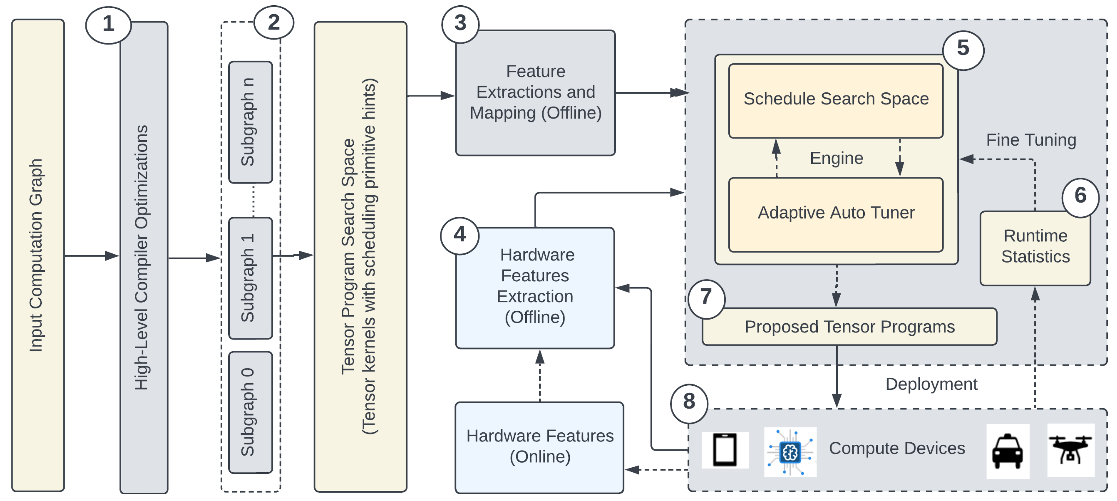
Figure 2.
Comparing Pairwise Comparison Accuracy Across Hardware
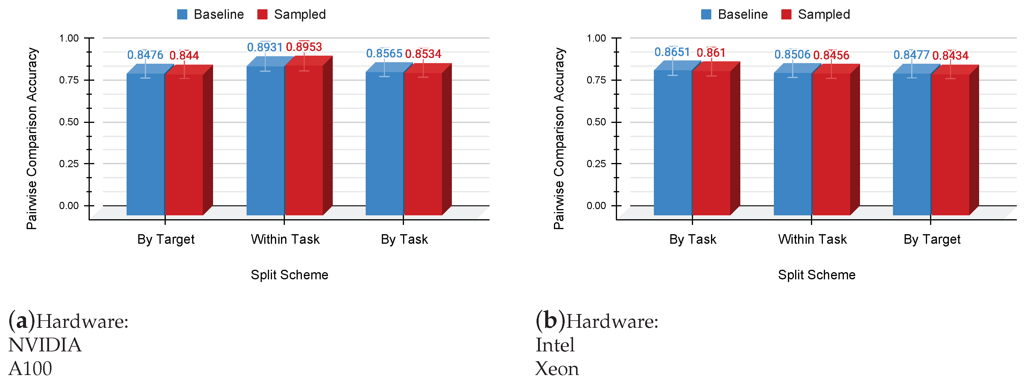
Figure 3.
Comparing Training Convergence of Tuners. *experimented on Nvidia RTX 2080
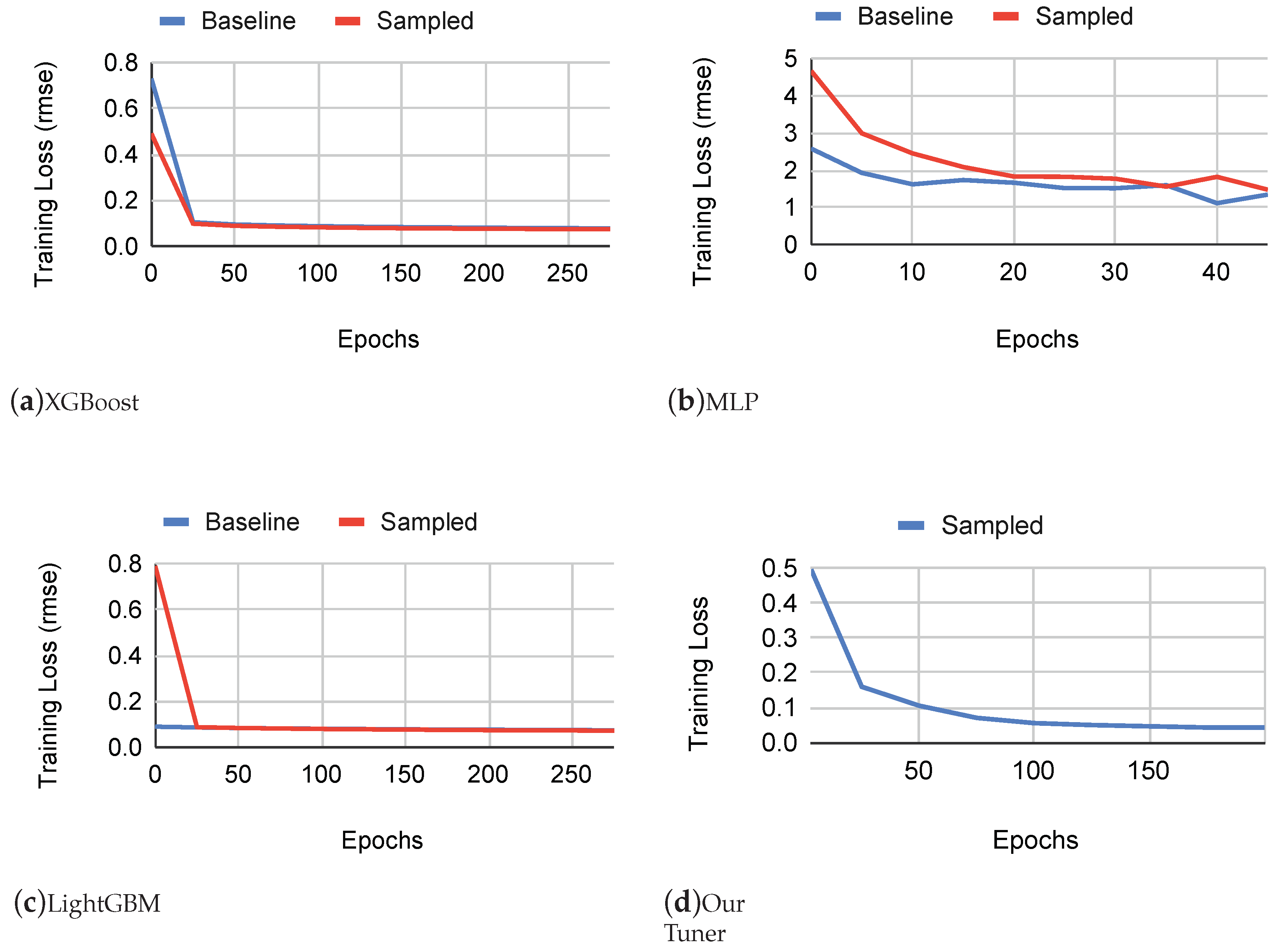

Table 1.
Compute Hardware Description
| Hardware Platform | Processor | Remarks |
|---|---|---|
| Intel Platinum 8272CL @ 2.60GHz | CPU | 16 cores, AVX-512 |
| AMD EPYC 7452 @ 2.35GHz | CPU | 4 cores, AVX-2 |
| ARM Graviton2 | CPU | 16 cores, Neon |
| NVIDIA Tesla T4 | GPU | Turing Architecture |
| NVIDIA GeForce RTX 2080 | GPU | Turing Architecture |
| NVIDIA A100 | GPU | Ampere Architecture |
| NVIDIA A40 | GPU | Ampere Architecture |
| NVIDIA H100 | GPU | Hopper Architecture |
| Intel Gold 5115 @ 2.40GHz | CPU | 40 cores, Xeon |
| ARM A64FX | CPU | 48 cores, aarch64 |
Table 2.
Hardware Parameters Considered While Training
| Hardware Parameter | Definition | Hardware Class | Value (bytes) |
|---|---|---|---|
| cache_line_bytes | chunks of memory handled by the cache | CPU; GPU | 64 |
| max_local_memory_per_block | maximum local memory per block in bytes | GPU | 2147483647 |
| max_shared_memory_per_block | maximum shared memory per block in bytes | GPU | 49152 |
| max_threads_per_block | maximum number of threads per block | GPU | 1024 |
| max_vthread_extent | maximum extent of virtual threading | GPU | 8 |
| num_cores | number of cores in the compute hardware | CPU | 24 |
| vector_unit_bytes | width of vector units in bytes | CPU; GPU | 64; 16 |
| warp_size | thread numbers of a warp | GPU | 32 |
Table 3.
Neural-Network And Hardware Features Characterization
| Sampled Kernels | #Kernel_Shapes | Max GFLOPs | Tensor Shape | Mean Execution Time (ms) | |||||
| CPU | GPU | CPU | GPU | EPYC-7452 | Graviton2 | Platinum-8272 | T4 | ||
| T_add | 229 | 388 | 8.59 | 8.59 | [4, 256, 1024] | 180.97 | 81.25 | 92.86 | 4.31 |
| Conv2dOutput | 60 | 27 | 1.20 | 1.07 | [4, 64, 64, 32] | 40.94 | 14.21 | 19.11 | 2.07 |
| T_divide | 24 | 69 | 0.003 | 0.003 | [8, 1, 1, 960] | 0.07 | 0.05 | 0.11 | 0.10 |
| T_fast_tanh | 9 | 9 | 0.008 | 0.008 | [4, 1024] | 0.43 | 0.43 | 0.53 | 0.97 |
| T_multiply | 105 | 150 | 8.92 | 8.92 | [4, 256, 4096] | 320.74 | 48.08 | 95.65 | 0.55 |
| T_relu | 300 | 1257 | 73.46 | 73.46 | [4, 144, 72, 8, 64] | 0.52 | 5.70 | 0.72 | 0.23 |
| T_softmax_norm | 27 | 27 | 0.016 | 0.016 | [4, 16, 256, 256] | 1.01 | 2.78 | 4.08 | 0.19 |
| T_tanh | 9 | 9 | 0.905 | 0.629 | [8, 96, 96, 3] | 5.55 | 33.48 | 50.55 | 0.16 |
| conv2d_winograd | 0 | 33 | NA | 0.868 | NA | NA | NA | NA | 0.93 |
*CPU: EPYC-7452, Graviton2, Platinum-8272; *GPU: T4; *NA: operator is not present in the considered CPU dataset **Measured on Nvidia GeForce RTX 2080
Table 4.
Auto-Tuner’s Hyperparameters
| Hyperparameter | Value |
|---|---|
| Batch | 16, 32, 64, 256, 512 |
| Epoch | 100, 200, 400 |
| Learning Rate | 1e-4 |
| Attention Head (fine tuning) | 6 |
| #Unrolling Steps for Attention Head | 2 |
| Optimizer | Adam |
Table 5.
Explanation of Scheduling Primitives
| Primitive | Meaning |
|---|---|
| AN | Annotation Step |
| FU | Fuse Step |
| PR | Pragma Step |
| RE | Reorder Step |
| SP | Split Step |
| FSP | Follow Split Step |
| FFSP | Follow Fused Split Step |
| SA | Storage Align Step |
| CA | Compute At Step |
| CI | Compute In-line Step |
| CR | Compute Root Step |
| CHR | Cache Read Step |
| CHW | Cache Write Step |
| RF | Rfactor Step |
Table 6.
Top 5 Scheduling Primitive’s Sequence Length and Probabilistic Occurrences
| H100 | A64FX | ||
| Sequence Length | Total Occurrence (%) | Sequence Length | Total Occurrence (%) |
| 37 | 46.41 | 21 | 20.89 |
| 36 | 12.59 | 20 | 20.21 |
| 39 | 5.56 | 16 | 11.06 |
| 38 | 5.00 | 17 | 8.91 |
| 32 | 4.62 | 19 | 7.29 |
Table 7.
Reduction In Dataset Size And Train-time (by split strategies)
| Target Hardware | Dataset | Size | XGBoost (train-time (sec)) | MLP (train-time (sec)) | LightGBM (train-time (sec)) | ||||||
| within_task | by_task | by_target | within_task | by_task | by_target | within_task | by_task | by_target | |||
| GPU | Baseline | 16G | 1504 | 1440 | 454 | 3000 | 2434 | 3150 | 1574 | 780 | 4680 |
| Sampled | 9G | 1406 | 1169 | 339 | 1968 | 1655 | 2464 | 1175 | 595 | 3637 | |
| CPU | Baseline | 11G | 1490 | 1265 | 428 | 3143 | 2623 | 2043 | 1131 | 636 | 3946 |
| Sampled | 6.8G | 905 | 780 | 354 | 2091 | 1672 | 1270 | 489 | 387 | 2435 | |
Table 8.
Inference Time Comparison (Seconds)
| Target Hardware | Baseline Dataset | Sampled Dataset | ||
| W/o Transfer Tuning | W/ Transfer Tuning | W/o Transfer Tuning | W/ Transfer Tuning | |
| A64FX (CPU) | 66.81 | 149.5 | 58.7 | 112.43 |
| Xeon (CPU) | 91.34 | 282.2 | 85.22 | 189.25 |
| A40 (GPU) | 627 | 416 | 599 | 175 |
| A100 (GPU) | 578 | 391 | 585 | 400 |
| H100 (GPU) | 128.12 | 67.30 | 93.42 | 54.25 |
| RTX2080 (GPU) | 18.67 | 27.68 | 17.37 | 841.74 |
Table 9.
Evaluation of Proposed Tuner: Variation In Tuning Time And Inference Time
| Target Hardware | Network | W/o Transfer Tuning | W/ Transfer Tuning | ||
| Time-to-Tune | Mean Inference Time | Time-to-Tune | Mean Inference Time | ||
| CPU | Incpetion_v3 | 614 | 75.27 | 61 | 73.80 |
| MobileNet_v3 | 236 | 5.48 | 71 | 5.57 | |
| ResNet_50 | 128 | 11.93 | 86 | 12.12 | |
| GPU | Incpetion_v3 | 2510 | 28.72 | 191 | 28.73 |
| MobileNet_v3 | 1092 | 1.72 | 136 | 1.75 | |
| ResNet_50 | 817 | 3.79 | 226 | 3.78 | |
*CPU: Intel Xeon; *GPU: A100; *w/o: without; w/: with; tune time (sec); inf time (ms)
Table 10.
Evaluation Of Proposed Tuner: Top-k Scores
| Target Hardware | TenSet XGB | Our Tuner | ||
| top-1 (%) | top-5 (%) | top-1 (%) | top-5 (%) | |
| H100 | 83.94 | 95.81 | 85.67 | 96.08 |
| A64FX | 72.6 | 92.49 | 77.04 | 91.79 |
*Network: ResNet_50
Disclaimer/Publisher’s Note: The statements, opinions and data contained in all publications are solely those of the individual author(s) and contributor(s) and not of MDPI and/or the editor(s). MDPI and/or the editor(s) disclaim responsibility for any injury to people or property resulting from any ideas, methods, instructions or products referred to in the content. |
© 2024 by the authors. Licensee MDPI, Basel, Switzerland. This article is an open access article distributed under the terms and conditions of the Creative Commons Attribution (CC BY) license (http://creativecommons.org/licenses/by/4.0/).
Copyright: This open access article is published under a Creative Commons CC BY 4.0 license, which permit the free download, distribution, and reuse, provided that the author and preprint are cited in any reuse.


