Submitted:
20 December 2023
Posted:
21 December 2023
You are already at the latest version
Abstract
Stratified Taylor Couette Flow (STCF) undergoes transient growth. Recent studies have shown that there exists transient amplification in the linear regime of counter-rotating STCF. It is reported that as Gr increases, the maximum amplification factor ($G_0$) initially decays before it eventually starts growing after reaching a certain critical value Gr$_{c}$. Assuming other parameters of the model are kept constant, the value Gr$_{c}$ changes with respect to different speed ratios of the cylinders. The observed decay/growth pattern of $G_0$ is attributed to the interplay between the induced shear and buoyancy. In this study, the mechanism that triggers this observed pattern is investigated. The kinetic budget of the optimal transient perturbation is analysed numerically to simulate the interaction of the shear production (SP), buoyancy production (BP) and other energy components that contributes to the total optimal transient kinetic energy. These contributions affect the total energy by influencing the perturbation to extract kinetic energy (KE) from the mean flow. The decay of $G_0$ resulted from the positive amplification of both BP and SP, while the growth is attributed to the negative and positive amplification of BP and SP, respectively. The optimal SP is positively amplified, implying that there is the possibility of constant linear growth. These findings agree with the linear growth rate for increasing values of Gr.
Keywords:
Bifurcation
; stability
; nonlinear dynamics
; Taylor-Couette flow
; convection
; buoyancy
; thermal diffusivity
1. Introduction
Counter rotating Stratified Taylor Couette Flow (STCF) is a complex fluid dynamics phenomenon that has attracted significant attention from researchers due to its relevance in various industrial and environmental applications. In recent years, numerous studies have been conducted to better understand the underlying mechanisms and characteristics of this flow regime [1,2]. Counter rotating Taylor Couette Flow refers to the flow of a fluid confined between two coaxial and independently rotating cylinders in opposite directions. This flow configuration has been extensively studied for decades and in recent times, primarily in the absence of stratification [3,4,5,6,7]. Conversely, in the presence of stratification the flow becomes more complex with more degrees of freedom in the parametric study of the dynamic behaviour [8,9]. Stratification refers to the presence of density gradients in the fluid, which can occur due to variations in temperature, salinity, or other properties.The buoyancy effect, resulting from the density differences caused by stratification, introduces a new dimension to the dynamics of STCF. It interacts with the rotational forces, and its impact on the stability of the flow has been the subject of considerable research interest [10,11,12,13,14,15,16,17,18].
A recent work by Godwin et al. [19] focussed specifically on the short-time instability of STCF. To explore the short-time instability of STCF, the authors conducted a detailed numerical investigation employing transient growth analysis techniques. The authors analyzed the transient stability of STCF by considering small perturbations superimposed on the base flow. By systematically varying the Grashof number for various model configurations, they were able to quantify the influence of these parameters on the transient instability characteristics. The study sheds light on the transient instability induced by buoyancy in counter rotating STCF within the bounds of the linear regime considered, but does not capture the physical mechanism that triggers the transient bifurcation phenomena at . The value is the critical value for which the transient bifurcation occurs with respect to the model configuration.
The primary goal of this study is to explore the physical processes responsible for triggering transient bifurcation, with specific objectives outlined as follows: developing a linear model for STCF and conducting a numerical evaluation using the Chebyshev collocation method, determining the least stable eigenvalue for each configuration, identifying the maximum amplification factor and optimal perturbation for the least stable mode, and ultimately deriving and evaluating the energy budget quantities associated with the optimal perturbation. This paper primarily focuses on the last objective, as the other aspects have already been satisfactorily addressed in previous work [19].
In Section 1, a brief overview of the investigated problem is presented to facilitate a thorough understanding of the topic. Section 2 focuses on deriving, linearizing, and numerically discretizing the governing equations of the STCF model. The discussion of optimal transient budget quantities is covered in Section 3, with detailed derivations provided in Appendix A. Section 4 delves into a comprehensive analysis of the investigation’s results. Finally, Section 5 summarizes the conclusions drawn from this study.
2. Mathematical Model
In this study, we consider an incompressible fluid between two concentric rotating heated vertical cylinders of infinite height. The inner cylinder has radius , rotates with an angular velocity of and is held at the temperature . The outer cylinder has radius , rotates with an angular velocity of and is held at the temperature . Here, is the ambient temperature, and is the temperature difference between the two cylinders. We assume that the density varies linearly with the temperature such that
where is the coefficient of thermal expansion. We assume that the dynamic viscosity of the fluid and thermal conductivity are constant, whilst we define as the kinematic viscosity. We notice we can write where .
The presence of temperature gradients with the rotating concentric cylinders induces complex flow patterns and thermal effects. The variation in the density, due to the temperature gradients, induces various buoyancy-driven flow regimes. The equations are nondimensionalised using
where , , , and are the dimensionless velocity, temperature, spatial coordinate, time and pressure, with . By defining we can express the dimensionless inner and outer radii as and , respectively. By dropping the accents for convenience, the resulting dimensionless equations become
where is the unit vector in the vertical axial direction and the Grashof number, Prandtl number and relative density are given by
The dimensionless boundary conditions are given as:
where is the unit vector in the azimuthal direction and the inner and outer Reynolds numbers are given by
Due to the cylindrical boundaries, we shall change to cylindrical polar coordinates. The steady base state velocity takes the form
In order to have a constant pressure gradient in the axial direction, we impose the zero mass flux constraint, namely
The well known analytical base state solution to this problem is given by
where the constants A, B and C are given by
and
Now, we consider small perturbations to the base state in the form
where is assumed to be a small constant, is the base state pressure, not presented here for convenience, and is the perturbation to the velocity. Substituting equation (12) into the dimensionless equations (2) to (4) and linearising in we obtain
To perform a stability analysis on this system we seek perturbations of the form
where and are the azimuthal and axial wavenumbers, respectively. Substituting these expansions into the linearized equations (13) - (15) and simplifying yields
where , and
By assuming a solution of the form:
we transform the initial value problem to a generalized eigenvalue problem:
The scalar eigenvalue is complex and defines the temporal stability of the flow. That is if the real part of is negative the flow is stable and the amplitude of the perturbations will decay in time. Conversely, if the real part of is positive the flow is unstable and the amplitude of the perturbation will grow asymptotically in time. Further more, in order to define the boundary conditions, we assume that the perturbation of the velocity and temperature of the fluid motion must vanish at the walls:
In other words, we impose homogeneous boundary condition for the velocity and temperature perturbations at the respective walls of the cylinders.
3. Perturbation Energy Budget
The asymptotic stability approach employed in perturbation analysis can effectively capture the length and time scales of unstable modes [20,21]. However, this method lacks an intuitive physical interpretation of the internal processes driving the instability. To gain a deeper understanding of the physical underpinnings of the instability, it is advantageous to adopt a more intuitive approach [22,23,24,25]. Exploring the processes influencing the kinetic energy distribution of perturbations can provide valuable insights [26,27,28].
The presence of kinetic energy in thermal stratified shear flow significantly impacts the perturbation’s decay or growth process [27,29]. The perturbation process is characterized by the conservation or transformation of energy across different states. For perturbations to grow, an energy exchange must occur. In the case of shear flow, perturbations grow by accessing kinetic energy. Investigating the quantities of energy sources interacting to form perturbation kinetic energy allows for a further understanding of the nature of induced instability—whether it is induced by shear or buoyancy—due to transient growing modes. When induced buoyancy is greater than zero, buoyant fluid rises near the wall, and dense fluid sinks. This process is also influenced by shear quantity. If the shear contribution of the energy source is less than zero, it implies that shear opposes induced convection due to buoyancy.
To calculate the kinetic energy of the optimal perturbation, we multiply the linearized equations (A1)-() by the complex conjugate of the optimal perturbation and evaluate the average over the entire domain in azimuthal and axial coordinating directions. This process yields the energy budget equation:
Please see appendix A for the derivation.
4. Result
Before delving into the discussion of our results, it’s important to acknowledge that in mixed convection flow, shear instability can manifest when there are relatively moving shear layers of fluid. The perturbations that arise from this instability may experience damping due to stable stratification because the perturbation’s energy must be expended to counteract the force of gravity induced by the stratification. Consequently, the growth rate of these perturbations will decrease, and the instability will be suppressed if the stratification is sufficiently strong. These intricate processes are elucidated through the examination of energy budget quantities within the framework of optimal transient perturbations, particularly in relation to the amplification factor, as elaborated upon in the subsequent sections.
The kinetic budget quantities of the optimal growth perturbation are numerical investigated for different stratified STCF configurations. In Table 1 the parameter values for the 4 different configurations are given.
The analysis is carried out with fixed values for Pr=68, =0.08, = 0.881, Re, and selected Gr. To obtain sufficiently accurate results, 128 Chebyshev nodes were used to compute the energy quantities.
The results are computed in a systematic manner. The least stable modes for each configuration are first identified followed by the optimal perturbation. The energy quantities are computed using the optimal disturbances as inputs for the selected Gr values. These values are chosen for illustrative purposes to show that the energy quantities oscillate between the cylinders before and after the turning points. For a more detailed discussion of these turning points please see Figure 4 in Godwin et al. [19].
Figure 1 illustrates energy quantities prior to the turning point for configurations and .
The terms KE, SP, BP, EF, CKEV, VD and BVP are defined in appendix A. We found that configurations and produced very similar results. The values of Gr are deliberately selected to be significantly smaller than the turning point, that is Gr . In the proximity of the outer cylinder wall, induced SP and BF draw KE from the mean flow into the perturbation, causing energy to radially flux inwards towards the center of the gap between the cylinders through EF. This energy, when spread by EF, converges/diverges at specific radial locations close to the outer cylinder wall. Moreover, Figure 1 reveals a sharp peak in KE near the outer cylinder wall due to the high values of SP and BF. The positive implication of BF indicates that buoyant fluid rises while dense fluid sinks near the outer cylinder wall. Conversely, the buoyancy flux resulting from the buoyancy variance in the heat equation is negatively amplified, albeit with a very small magnitude of about .
Figure 2 depicts energy quantities around the turning point for configurations and .
We found that configurations and produced very similar results. Depending on the Gr values around this point, the kinetic energy (KE) exhibits a concentrated distribution of significant peaks either towards the outer or inner cylinder, with a minor bump on the tail side of the amplitude. No specific value was identified while varying the Gr values across the transition from the decaying to the growth phase of the amplification factor, , due to transient discontinuity around the turning point. Additionally, the energy flux (EF) displays converging/diverging peaks, with one peak being more pronounced than the other in relation to the Gr value near that point. This suggests that EF evenly spreads the energy from the center to the cylinder walls.
Figure 3 illustrates energy quantities beyond the turning point for configurations and .
We found that configurations and produced very similar results. The values of Gr have been selected to be significantly larger than the turning point, denoted as Gr . Near the wall of the inner cylinder, the induced SP and BF extract KE from the mean flow into the perturbation, causing the energy to flux radially inwards towards the center of the inner cylinders through EF. The spreading of energy by EF leads to convergence/divergence at specific radial locations near the wall, . Additionally, Figure 3 also shows a sharp peak in KE near due to the high concentration of SP and BF. The negative implication of BF implies that shear-induced instability must exert more work against gravity to grow by suppressing buoyant fluid and lifting dense fluid near . Conversely, the buoyancy flux resulting from the buoyancy variance in the heat equation is positively amplified, albeit with a very small magnitude of about .
The opposite signs of the amplitude of BP and SP may trigger showtime or long-time instability depending on the proportionality of magnitude of each amplification. We see that has because the disparity between the SP and BP values differed significantly it tends to cause a short time amplification. However, for a sufficiently high value of BP, the short time amplification dies as shown in Figure 4.
This long-time behaviour is what is capture by the asymptotic analysis of the eigenvalue. Although, it can be tempting to conclude that buoyancy is the trigger for the short time instability, but we argue otherwise, that it this the shear drag as it opposes the buoyancy to triggers the short time instability as evident in the long time run captured in Figure 4.
The viscous processes (CKEV and VD) is unable to generate the optimal perturbation kinetic energy (KE) akin to the energy flux (EF). Instead, these viscous terms disperse energy without adding to the overall KE, and they vanish at the boundaries. The dissipative terms (VD) exhibit a negative definiteness, leading to the decay of KE. It’s worth noting that viscosity functions as an energy sink for the perturbation, compelling the velocity at the boundary to gradually diminish to zero. This process results in a distortion of the perturbation, causing the wall-normal velocity () of the perturbation to incline against the transient background shear shown in Figure 4, ultimately yielding a positive shear production (SP) amplification. While viscosity doesn’t directly contribute to KE, it indirectly influences it by configuring the perturbation in a manner that enables it to extract KE from the background mean flow.
In Figure 5 we illustrate the vertical vorticity for the four configurations.
In Figure 5, the left column (for values of Gr before the turning point), shows that the largest variations in the vertical vorticity are in the region near the outer cylinder, however, the right column (for values of Gr after the turning point), shows that the largest variations in the vertical vorticity are in the region near the inner cylinder.
In Figure 6 we illustrate the horizontal velocity in the z plane.
Figure 6, the left column (for values of Gr before the turning point), shows that the largest variations in the horizontal velocity are in the region near the outer cylinder, however, the right column (for values of Gr after the turning point), shows that the largest variations in the horizontal velocity are in the region near the inner cylinder.
In Figure 7 we illustrate the vertical velocity in the azimuthal plane.
Figure 7, the left column (for values of Gr before the turning point), shows that the largest variations in the vertical velocity are in the region near the outer cylinder, however, the right column (for values of Gr after the turning point), shows that the largest variations in the vertical velocity are in the region near the inner cylinder.
5. Conclusion
The complex dynamics of mixed convection flow with a particular focus on shear instability and its manifestation in the presence of stratified conditions is investigated further in this paper. The analysis involves a systematic numerical investigation of kinetic budget quantities for optimal growth perturbations in various stratified configurations of Taylor-Couette flow. The key findings shed light on the interplay of different energy components and their effects on the transient growth.
The results reveal distinct behaviours of energy quantities before, around, and beyond the turning point in the amplification factor. Prior to the turning point, the values of shear production (SP) and buoyancy flux (BF) near the outer cylinder wall induces significant kinetic energy (KE) peaks. This positive amplification of BF indicates a buoyant fluid rise, while the negative amplification suggests shear-induced instability opposing gravity. Around the turning point, the kinetic energy distribution exhibits peaks either toward the outer or inner cylinder, emphasizing the transient nature of the amplification process. Beyond the turning point, the energy quantities show similar amplification peaks, with SP and BF near the inner cylinder wall causing significant KE peaks.
The analysis also highlights the role of buoyancy and shear drag in triggering short-time and long-time instability. The disparity between BF and SP values significantly influences the nature of amplification, with a sufficiently high shear production leading to the decay of short-time amplification. This long-time behavior is captured by asymptotic analysis of the eigenvalue. Contrary to initial assumptions, the study argues that shear drag, rather than buoyancy, is the primary trigger for short-time instability.
Furthermore, the viscous processes (CKEV and VD) are found to disperse energy without contributing to the overall KE, while dissipative terms (VD) lead to the decay of KE. Viscosity acts as an energy sink, gradually diminishing the velocity at the boundary and influencing the perturbation’s configuration to extract KE from the background mean flow.
In summary, our analysis provides insight into the intricate processes governing mixed convection flow with shear instability, emphasizing the role of buoyancy, shear drag, and viscosity in shaping the flow dynamics. These findings contribute to a deeper understanding of the underlying mechanisms in complex fluid systems.
Author Contributions
Conceptualization, L.E. Godwin; methodology, L.E. Godwin; software, L.E. Godwin; validation, L.E. Godwin; formal analysis, L.E. Godwin; investigation, L.E.Godwin, S.C. Generalis; resources, L.E. Godwin and S.C. Generalis; writing—original draft preparation, L.E. Godwin; writing—review and editing, L.E. Godwin, P.M.J. Trevelyan, T. Akinaga and S.C. Generalis; supervision, P.M.J. Trevelyan, S.C. Generalis; project administration, P.M.J. Trevelyan and S.C. Generalis; funding acquisition, L.E. Godwin and S.C. Generalis. All authors have read and agreed to the published version of the manuscript.
Funding
This research was funded by RISE Horizon 2020 ATM2BT, Atomistic to Molecular Turbulence, Grant no 824022, TETFUND scholarship and DTI EPSRC grant, Aston University sponsorship.
Data Availability Statement
The Matlab sources codes used to generate the data in this study can be made available upon request.
Acknowledgments
We would like to thank Dr. Samesa Igirigi and Dr. Hart Abarasi for many fruitful discussions.
Conflicts of Interest
The authors declare no conflict of interest.
Appendix A Derivations of Optimal Perturbation Energy Budget Equation
Firstly we repose equation (1) as a NVE of the optimal perturbation, and then we proceed by taking the inner product with the optimal perturbation in component wise as follows :
If we multiply each of the first 3 equations by the associated velocity component and then take the sum of these we can obtain
Now we integrate over the axial and azimuthal directions and assume periodic boundary conditions in both those directions to give
where denotes the average given by . If we multiply equation (A4) by and average as before we obtain
Now the conservation of mass equation is given by
If we multiply equation (A6) by then integrate over the axial and azimuthal directions, and then add this equation to equation (A5) we obtain
where the terms are defined as follows:
where the kinetic energy of the perturbation is KE, the shear production is SP, the buoyancy production is BP, the energy flux is EF, CKEV convergence of kinetic energy of the optimal perturbation due to viscosity, VD is viscosity dissipation and BVP is the buoyancy variance.
References
- Bengana, Y.; Tuckerman, L. Spirals and ribbons in counter-rotating Taylor-Couette flow: Frequencies from mean flows and heteroclinic orbits. Phys. Rev. Fluids 2019, 4, 044402. [Google Scholar] [CrossRef]
- Obaidullah, K.; Baig, M.; Sanghi, S. Counter-rotating Taylor-Couette flows with radial temperature gradient. Int. J. Heat and Fluid Flow 2022, 95, 108980. [Google Scholar] [CrossRef]
- Hamede, M.; Merbold, S.; Egbers, C. Experimental investigation of turbulent counter-rotating Taylor-Couette flows for radius ratio η=0.1. J. Fluid Mech. 2023, 964, A36. [Google Scholar] [CrossRef]
- Wang, B.; Ayats, R.; Deguchi, K.; Mellibovsky, F.; Meseguer, A. Self-sustainment of coherent structures in counter-rotating Taylor–Couette flow. J. Fluid Mech. 2022, 951, A21. [Google Scholar] [CrossRef]
- Avila, K.; Hof, B. Second-Order Phase Transition in Counter-Rotating Taylor-Couette Flow Experiment. Entropy 2021, 23. [Google Scholar] [CrossRef] [PubMed]
- Huisman, S.; Lohse, D.; Sun, C. Statistics of turbulent fluctuations in counter-rotating Taylor-Couette flows. Phys. Rev. E 2013, 88, 063001. [Google Scholar] [CrossRef] [PubMed]
- Coles, D. Transition in circular Couette flow. J. Fluid Mech. 1965, 21, 385–425. [Google Scholar] [CrossRef]
- Boubnov, B.; Gledzer, E.; Hopfinger, E. Stratified circular Couette flow: instability and flow regimes. J. Fluid Mech. 1995, 292, 333–358. [Google Scholar] [CrossRef]
- Boubnov, B.; Gledzer, E.; Hopfinger, E.; Orlandi, P. Layer formation and transitions in stratified circular Couette flow. Dynamics of atmospheres and oceans 1996, 23, 139–153. [Google Scholar] [CrossRef]
- Lopez, J.M.; Lopez, J.M.; Marques, F. Stably stratified Taylor–Couette flows. Phil. Trans. Royal Soc. A 2023, 381, 20220115. [Google Scholar] [CrossRef]
- Lopez, J.; Marques, F. Three-dimensional instabilities in a discretely heated annular flow: Onset of spatio-temporal complexity via defect dynamics. Phys. Fluids 2014, 26. [Google Scholar] [CrossRef]
- Lopez, J.; Marques, F.; Avila, M. The Boussinesq approximation in rapidly rotating flows. J. Fluid Mech. 2013, 737, 56–77. [Google Scholar] [CrossRef]
- Caton, F.; Janiaud, B.; Hopfinger, E. Stability and bifurcations in stratified Taylor–Couette flow. J. Fluid Mech. 2000, 419, 93–124. [Google Scholar] [CrossRef]
- Molemaker, M.; McWilliams, J.; Yavneh, I. Instability and equilibration of centrifugally stable stratified Taylor-Couette flow. Phys. Rev. Letts. 2001, 86, 5270. [Google Scholar] [CrossRef] [PubMed]
- Caton, F.; Janiaud, B.; Hopfinger, E. Primary and secondary Hopf bifurcations in stratified Taylor-Couette flow. Phys. Rev. Lett. 1999, 82, 4647. [Google Scholar] [CrossRef]
- Hua, B.; Le Gentil, S.; Orlandi, P. First transitions in circular Couette flow with axial stratification. Phys. Fluids 1997, 9, 365–375. [Google Scholar] [CrossRef]
- Hua, B.; Moore, D.; Le Gentil, S. Inertial nonlinear equilibration of equatorial flows. J. Fluid Mech. 1997, 331, 345–371. [Google Scholar] [CrossRef]
- Thorpe, S. The stability of stratified Couette flow. Notes on 1966, pp. 80–107.
- Godwin, L.; Trevelyan, P.M.J.; Akinaga, T.; Generalis, S. Transient Dynamics in Counter-Rotating Stratified Taylor–Couette Flow. Mathematics 2023, 11. [Google Scholar] [CrossRef]
- Strogatz, S.H. Nonlinear Dynamics and Chaos: With Applications to Physics, Biology, Chemistry and Engineering, third ed.; CRC Press, 2000. [Google Scholar]
- Stuart, J.T. Hydrodynamic Stability. By P. G. Drazin and W. H. Reid. Cambridge University Press, 1981. 525 pp. J. Fluid Mech. 1982, 124, 529–532. [Google Scholar] [CrossRef]
- Schmid, P.J.; Brandt, L. Analysis of Fluid Systems: Stability, Receptivity, Sensitivity: Lecture notes from the FLOW-NORDITA Summer School on Advanced Instability Methods for Complex Flows, Stockholm, Sweden, 2013. Applied Mechanics Reviews 2014, 66, 024803. [Google Scholar] [CrossRef]
- Meseguer, A. Energy transient growth in the Taylor-Couette problem. Phys. Fluids 2002, 14, 1655–1660. [Google Scholar] [CrossRef]
- Reddy, S.C.; Henningson, D.S. Energy growth in viscous channel flows. J. Fluid Mech. 1993, 252, 209–238. [Google Scholar] [CrossRef]
- Trefethen, L.N.; Trefethen, A.E.; Reddy, S.C.; Driscoll, T.A. Hydrodynamic stability without eigenvalues. Science 1993, 261, 578–584. [Google Scholar] [CrossRef] [PubMed]
- Dandoy, V.; Park, J.; Augustson, K.; Astoul, A.; Mathis, S. How tidal waves interact with convective vortices in rapidly rotating planets and stars. A & A 2023, 673, A6. [Google Scholar] [CrossRef]
- Lian, Q.; Smyth, W.; Liu, Z. Numerical Computation of Instabilities and Internal Waves from In Situ Measurements via the Viscous Taylor–Goldstein Problem. J. Atmospheric and Oceanic Tech. 2020, 37, 759–776. [Google Scholar] [CrossRef]
- Lin, S.P. Roles of surface tension and Reynolds stresses on the finite amplitude stability of a parallel flow with a free surface. J. Fluid Mech 1970, 40, 307–314. [Google Scholar] [CrossRef]
- Smyth, W.D.; Carpenter, J.R. Instability in Geophysical Flows; Cambridge University Press, 2019. [Google Scholar] [CrossRef]
Figure 1.
The optimal perturbation energy budget quantities. The configurations (top) and (bottom) are for selected values of Gr before the turning points.
Figure 1.
The optimal perturbation energy budget quantities. The configurations (top) and (bottom) are for selected values of Gr before the turning points.
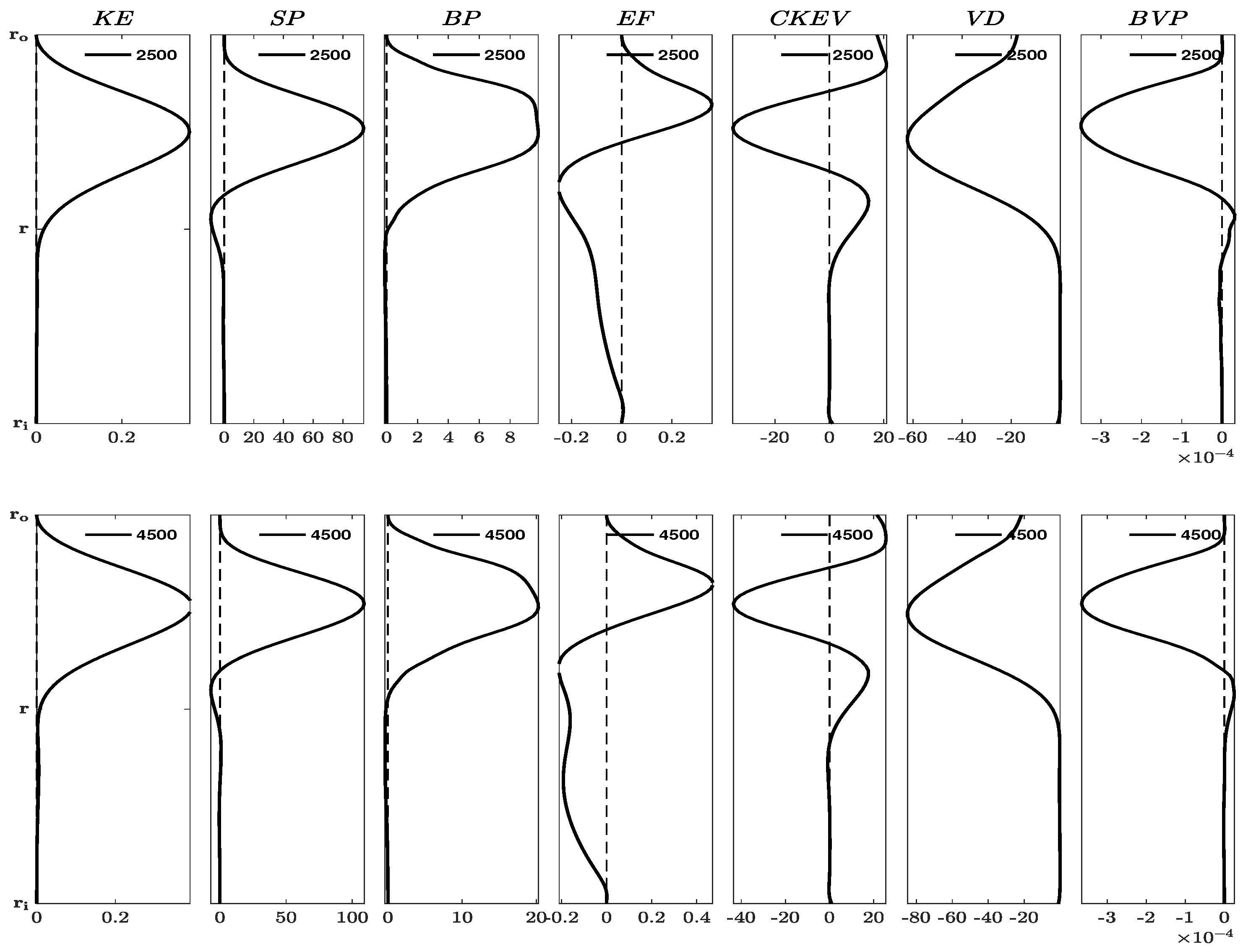
Figure 2.
The optimal perturbation energy budget quantities. The configurations (top) and (bottom) are for selected values of Gr about the turning points.
Figure 2.
The optimal perturbation energy budget quantities. The configurations (top) and (bottom) are for selected values of Gr about the turning points.
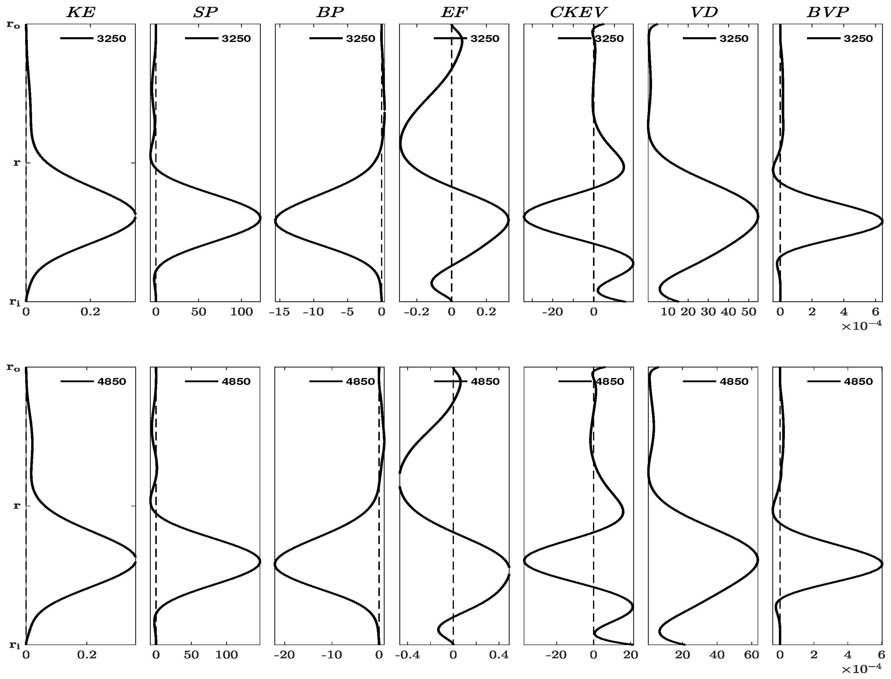
Figure 3.
The optimal perturbation energy budget quantities. The configurations (top) and (bottom) are for selected values of Gr after the turning points.
Figure 3.
The optimal perturbation energy budget quantities. The configurations (top) and (bottom) are for selected values of Gr after the turning points.
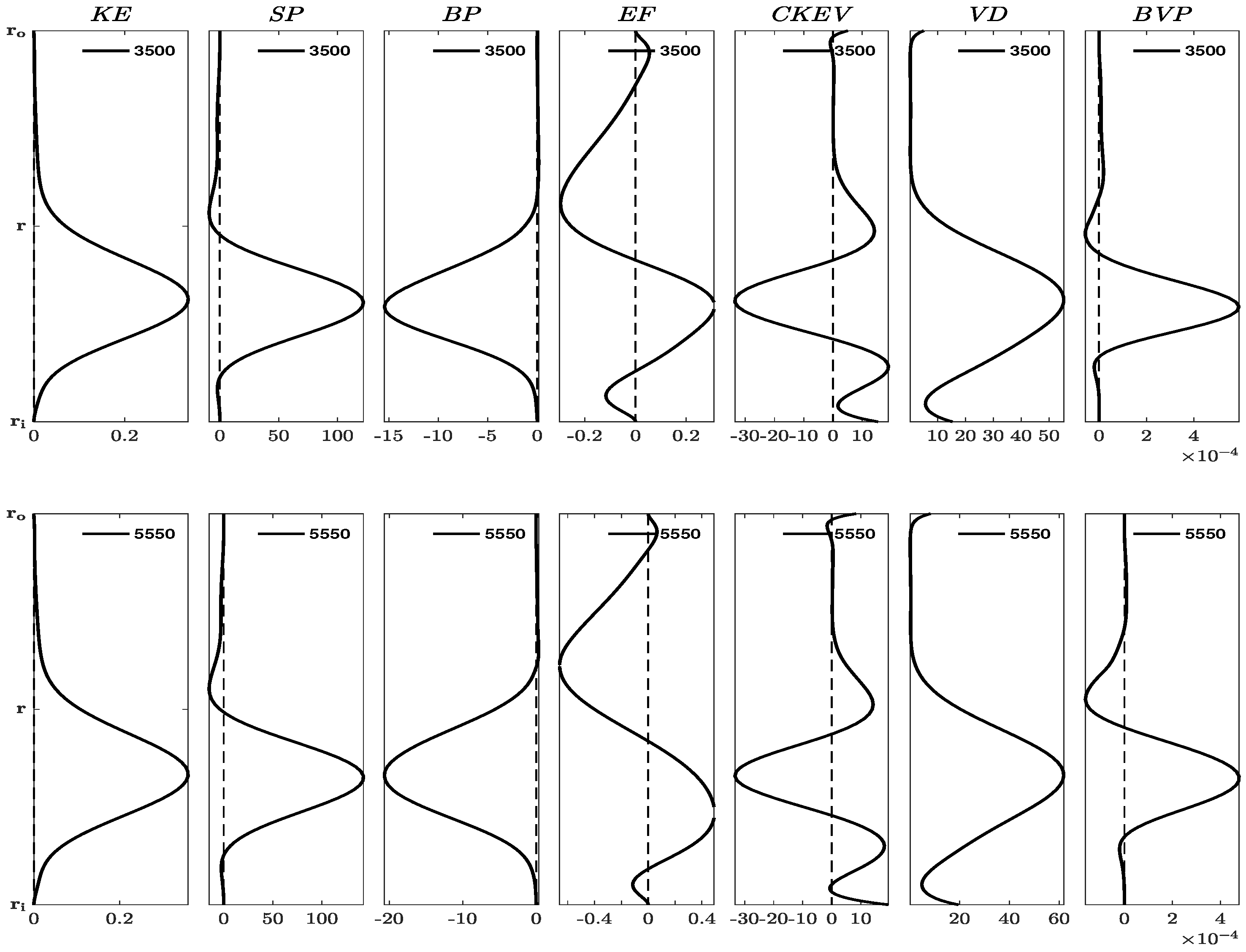
Figure 4.
The wall-normal velocity of the optimal perturbation. Configurations , , , and are organized in rows from top to bottom, for selected Gr values. The columns correspond to points before, around, and after the turning points.
Figure 4.
The wall-normal velocity of the optimal perturbation. Configurations , , , and are organized in rows from top to bottom, for selected Gr values. The columns correspond to points before, around, and after the turning points.
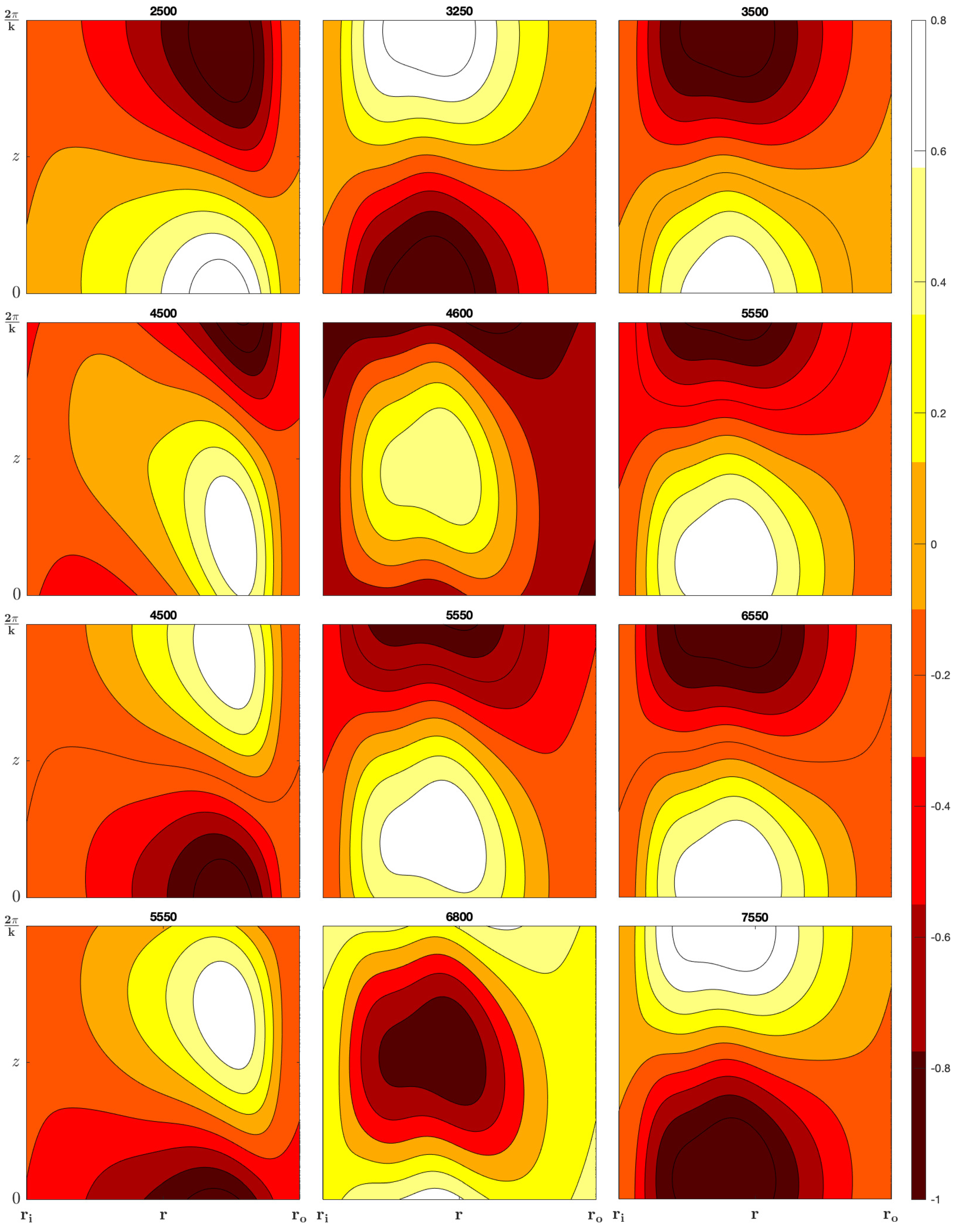
Figure 5.
The vertical vorticity of the optimal perturbation. Configurations , , , and are organized in rows from top to bottom, for selected Gr values. The columns correspond to points before, around, and after the turning points.
Figure 5.
The vertical vorticity of the optimal perturbation. Configurations , , , and are organized in rows from top to bottom, for selected Gr values. The columns correspond to points before, around, and after the turning points.
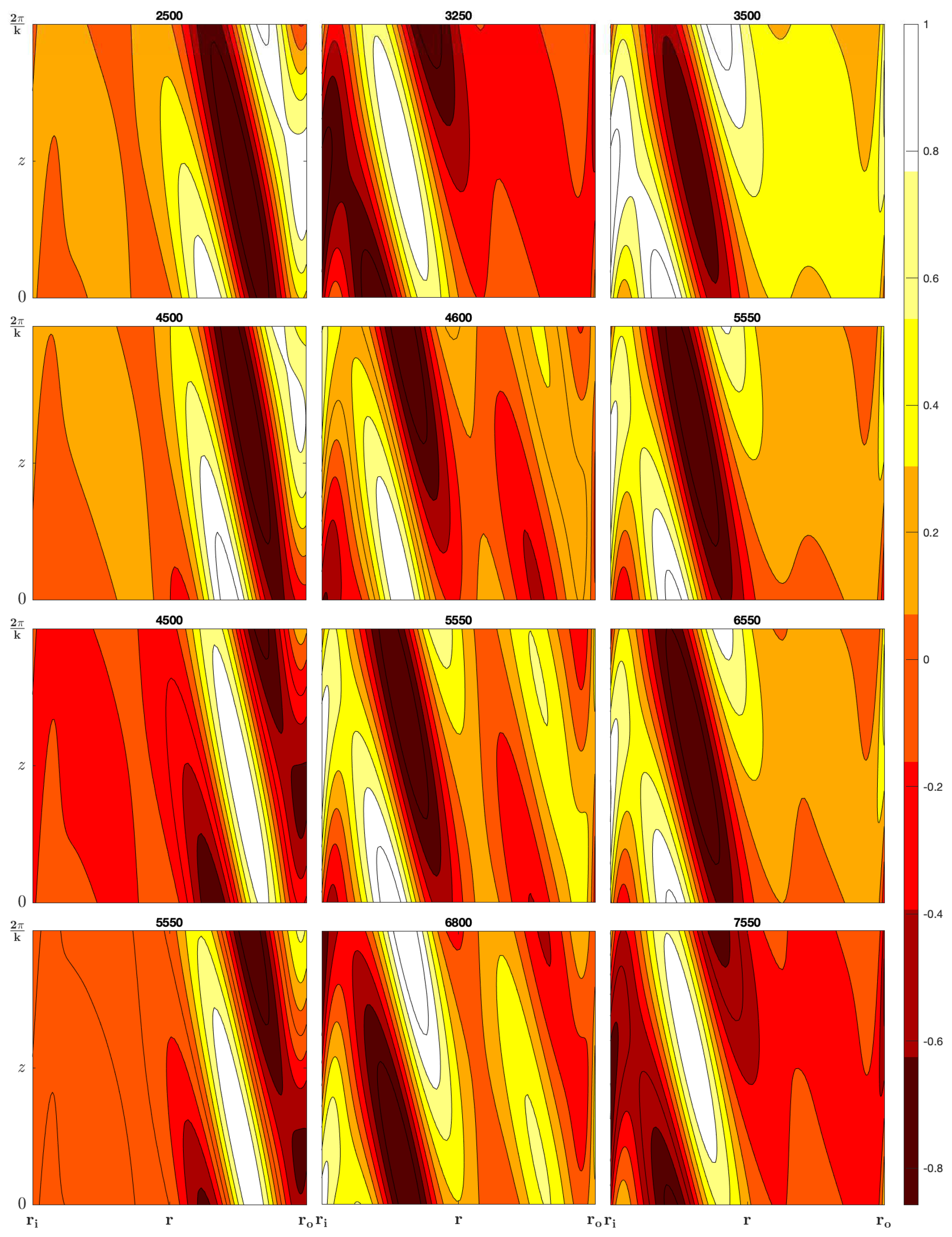
Figure 6.
The horizontal velocity of the optimal perturbation. Configurations , , , and are organized in rows from top to bottom, for selected Gr values. The columns correspond to points before, around, and after the turning points.
Figure 6.
The horizontal velocity of the optimal perturbation. Configurations , , , and are organized in rows from top to bottom, for selected Gr values. The columns correspond to points before, around, and after the turning points.
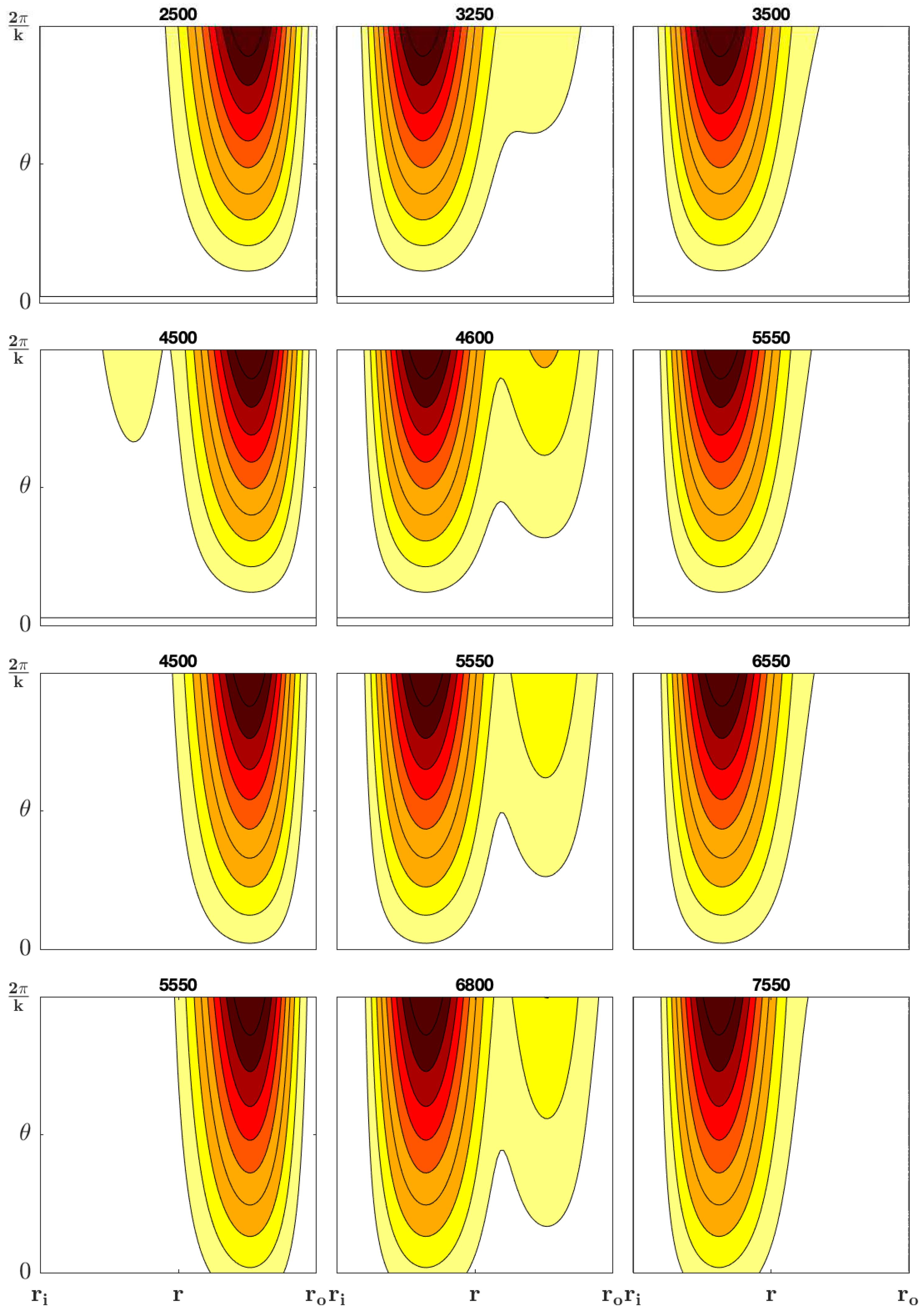
Figure 7.
The vertical velocity of the optimal perturbation. Configurations , , , and are organized in rows from top to bottom, for selected Gr values. The columns correspond to points before, around, and after the turning points.
Figure 7.
The vertical velocity of the optimal perturbation. Configurations , , , and are organized in rows from top to bottom, for selected Gr values. The columns correspond to points before, around, and after the turning points.
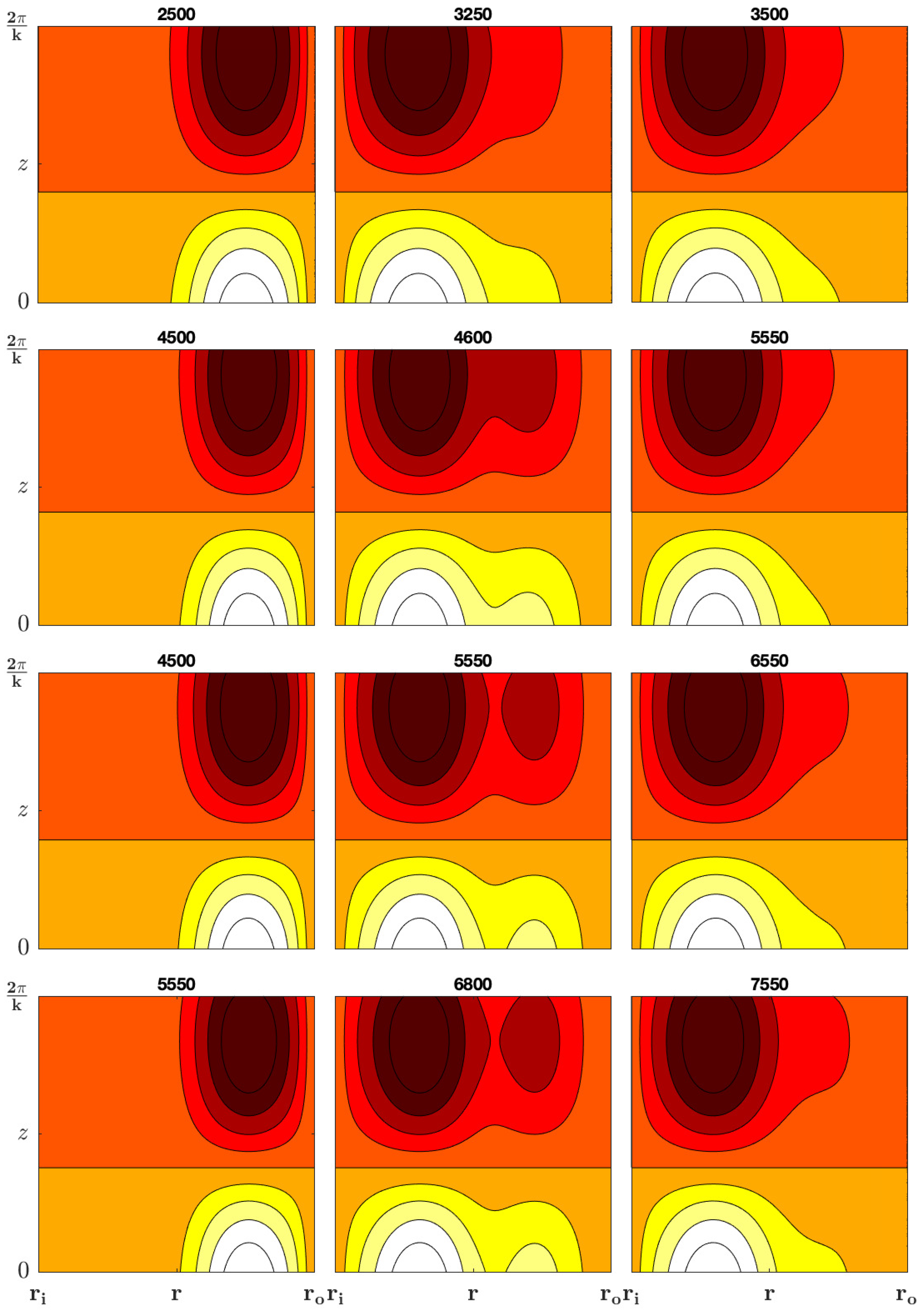

Table 1.
This table displays the 4 configurations examined in Godwin et al. (2023).
| Config | Ratio | n | k | ||
|---|---|---|---|---|---|
| 591 | 1:4 | 10 | 1.9940 | ||
| 523 | 1:6 | 11 | 1.9960 | ||
| 473 | 1:8 | 11 | 1.9200 | ||
| 405 | 1:9 | 11 | 1.8390 |
Disclaimer/Publisher’s Note: The statements, opinions and data contained in all publications are solely those of the individual author(s) and contributor(s) and not of MDPI and/or the editor(s). MDPI and/or the editor(s) disclaim responsibility for any injury to people or property resulting from any ideas, methods, instructions or products referred to in the content. |
© 2023 by the authors. Licensee MDPI, Basel, Switzerland. This article is an open access article distributed under the terms and conditions of the Creative Commons Attribution (CC BY) license (http://creativecommons.org/licenses/by/4.0/).
Copyright: This open access article is published under a Creative Commons CC BY 4.0 license, which permit the free download, distribution, and reuse, provided that the author and preprint are cited in any reuse.


