

Submitted:
08 December 2023
Posted:
12 December 2023
You are already at the latest version
Abstract
This research provides a computationally efficient numerical tool for predicting 3-D turbulent flows over hydrofoils. It addresses a gap in existing numerical methods by extending the capabilities of the laminar VIScous Vorticity Equation (VISVE) solver to handle 3-D turbulent flow scenarios. The implementation integrates the k − ω SST model into the 3-D VISVE solver using the Finite Volume Method (FVM), extending its capability to handle turbulent flows. The turbulence model is also parallelized to improve computational efficiency. The application of the newly developed model to 3-D hydrofoil cases expands its scope and serves as preparatory work for future rotational propeller applications. Rigorous testing includes a convergence analysis concerning grid numbers and time step sizes, and validation against a Reynolds-Averaged Navier-Stokes (RANS) solver ensures the reliability and accuracy of the enhanced VISVE solver for turbulent flow simulations. The turbulent VISVE solver offers advantages such as reduced computational domain and costs through a vorticity-based approach. Turbulence concentration within boundary layers and free shear flows does not compromise the advantages of the small computational domain. The simplified meshing process, automatically generated by denoting the number of panels on the hydrofoil, makes the solver accessible for researchers and engineers.
Keywords:
Software Development
; Viscous Vorticity Equation
; Turbulence Modeling
; 3-D Hydrofoil
; Computational Fluid Dynamics
1. Introduction
Marine propellers, crucial for ship, boat, and submarine propulsion, face challenges in turbulent flows affecting thrust, torque, noise, and durability. Accurate prediction and understanding of propeller behavior in turbulent flows are essential for analysis and design. Developing reliable computational models becomes crucial for accurately predicting propeller performance in complex flow phenomena. Foundational understanding from hydrofoils aids in comprehending fluid dynamics and lift generation, essential for propeller design and advancing propulsion knowledge.
In the realm of marine propeller simulations, challenges arise due to several reasons. Computational Fluid Dynamics (CFD) simulations face complexities in handling the computational domain size for these large propellers, impacting cost and time considerations. Turbulence modeling becomes crucial to accurately capture complex turbulent flow patterns induced by large propellers, involving separation, vortices, and cavitation. The intricate interactions between propeller blades and the hull, as well as blade-blade interactions, pose modeling challenges, necessitating specialized techniques. Mesh generation for complex geometries like large propellers demands time and expertise, while validation against experimental data is hindered by challenges in achieving high Reynolds numbers and obtaining reliable data for large-scale flows. These challenges underscore the need for specialized computational tools in addressing the marine propeller simulations.
The numerical methods for propeller analysis include the Vortex Lattice Method (VLM), Boundary Element Method (BEM), Computational Fluid Dynamics (CFD), and Viscous/Inviscid Interactive Method. VLM, a semi-analytical approach, models hydrodynamic surfaces through vortex panels, proving efficient for inviscid flow analysis due to its computational effectiveness. Its application to fully wetted propeller flows evolved into the MPUF-3A code, incorporating features like leading-edge correction [1,2,3,4,5,6,7]. BEM, another semi-analytical method, solves Partial Differential Equations on boundaries and gained traction in propeller analysis through codes like PROPCAV, allowing for the study of unsteady cavitating flow [8,9,10,11,12,13,14]. Additionally, the boundary layer strip theory simplifies viscous flow modeling [15,16,17,18]. CFD packages such as ANSYS Fluent [19], Siemens Star-CCM+ [20], and the open-source solution OpenFOAM [21] are widely used.
While conventional linear and potential flow theories offer computational efficiency, they exhibit limitations in accurately predicting turbulent flows. On the other hand, viscous flow methods, which can handle turbulence through the incorporation of a turbulence model, often being computationally intensive.
The primary objective of this research is to develop a computationally efficient viscous numerical model capable of accurately predicting the 3-D hydrofoil in turbulent flow conditions. The focus of the research is to extend the VISVE solver, originally designed for laminar flows, to handle turbulent flow scenarios.
VISVE stands for and it is a numerical solver developed in the Ocean Engineering Group at the University of Texas at Austin. VISVE focuses on solving the transport equation for vorticity. In VISVE, the flow variables are represented primarily in terms of vorticity rather than the traditional velocity and pressure fields, as done in the N-S solver.
VIScous Vorticity Equation (VISVE) has been solved by using a finite volume method ([22,23]). [23] developed the VISVE solver for laminar flows. Laminar VISVE has been applied on 2-D and 3-D hydrofoils, circular cylinders, and propeller blades (see [22], [24], [25] and [26]). Comprehensive parallelization using MPI and OpenMP hybrid programs is accomplished by [27]. [28] and [29] consider the compressibility and implement the laminar cavitating flow for VISVE. [30] derived the vorticity equation for turbulent compressible flows with variable viscosity. [31] and [32] coupled VISVE with a turbulence model in OpenFOAM, to solve the turbulent flow around a 2-D hydrofoil and cylinder. However, this coupling method did not solve for the turbulence in VISVE, and needed to read the turbulent viscosity from OpenFOAM at every time step, which meant that the VISVE solver could not solve the turbulent flow independently. This gap is filled by You and Kinnas [33]. The turbulent SST model is discretized and solved within the VISVE code, thus solving for turbulent flows independently [33]. The 2-D turbulent VISVE solver is applied to hydrofoils cases [33] and cylinder cases [34].
Prior work on VISVE has primarily focused on laminar flows and 2-D turbuelnt flows, it lacks coverage of 3-D turbulent cases, indicating a notable gap in existing numerical methods.
This research aims to bridge this gap by extending the capabilities of the VISVE solver to handle 3-D turbulent flow scenarios. To achieve this, this paper focuses on the following work:
- Software Development: The k-omega SST model has been successfully integrated into the 3-D VISVE solver based on the Finite Volume Method (FVM). This numerical implementation extended the solver’s capability to handle turbulent flows.
- Parallelization of the Turbulence Model: Another development involves the parallelization of the turbulence model within the VISVE solver. This enhanced the computational efficiency for turbulent flows.
- Application to 3-D Hydrofoil Cases: The implemented model has been applied to 3-D hydrofoil cases, thereby expanding the solver’s applicability. This application also serves as preparatory work before its application to rotational propeller.
- Convergence Test and Validation: The newly developed model undergoes a convergence analysis concerning grid numbers and time step sizes. Results obtained for various angles of attack, Reynolds numbers, and unsteady and steady states are validated against a RANS solver. This process ensures the reliability and accuracy of the enhanced VISVE solver for turbulent flow simulations.
The development of the turbulent VISVE solver addresses a gap in existing numerical methods, offering reduced computational cost through a vorticity-based approach. The turbulent VISVE numerical solver, designed for handling turbulent flows over hydrofoils and propellers, boasts several advantages.
- Due to the rapid reduction of vorticity away from the wall, this method requires significantly fewer grids and unknowns compared to velocity-based approaches, enhancing computational efficiency. Turbulence concentration within boundary layers and free shear flows does not compromise the advantage of the small computational domain.
- The small computational domain also simplifies the meshing process. Mesh generation is user-friendly, automatically generated by denoting the number of panels on the hydrofoil, making it accessible for researchers and engineers.
- The pressure term is eliminated in VISVE. Without coupling the pressure with the velocity, pressure can be calculated by a post-processing scheme.
- The solver incorporates the influence of the image of the half wing on the key half wing by considering the vorticity and velocity as identical on both. This approach deviates from periodic conditions because it ensures validity in both uniform and non-uniform flow conditions.
This paper begins with an introduction highlighting the gap in addressing 3-D turbulent cases in previous VISVE work. It leads to methodology section, discussing the extension of the VISVE solver and the implementation of the turbulence model. Application to 3-D hydrofoil cases is detailed, followed by convergence tests and result validation with a RANS solver. The paper concludes by summarizing contributions and suggesting future research directions.
2. Methodology and Numerical Implementations
In this section, the methodology and numerical models are presented. In general, the VISVE code relies on the Finite Volume Method (FVM). It comprises three main components: the vorticity solver, the velocity solver, and the turbulence solver.
To address turbulent flow, three significant enhancements to the existing laminar VISVE solver are necessary. Firstly, modifications must be made to the vorticity equation to account for turbulence effects. Additionally, the SST turbulence model, comprising a pair of second-order partial differential equations, should be resolved using the FVM. Furthermore, capturing turbulence features necessitates small grid resolutions and time scales. Parallelization of the turbulence model becomes crucial to efficiently handle the computational demands. These three aspects are introduced for the first time in this paper and have not been addressed in previous research.
2.1. Methodology
This section will elucidate the equations governing the flow. Both the vorticity and velocity solvers have been modified to account for the inclusion of turbulence effects. In addition, the turbulence model is newly developed into the 3-D code. The modifications, in comparison to the previous laminar model, will be highlighted when presenting these models.
2.1.1. 3-D Viscous Vorticity Equation
The viscous vorticity equation was derived by taking curl of the Navier-Stokes Equation. The 3-D VISVE Equation for variable density and viscosity is derived by [35]:
where stands for the vorticity; represents the velocity vector; is the kinematic viscosity, which can be taken as the summation of , where is the kinematic molecular viscosity and is the kinematic turbulent viscosity of the fluid.
For hydrofoil cases, with , where can represent any variable, Equation (1) can be simplified as:
In comparison to the vorticity equation for laminar flow, as shown by Equation (3), a notable distinction in the vorticity equation lies in the inclusion of the kinematic viscosity term () inside the curl operator. This significant difference can lead to substantial variations in the obtained results.
Taking the curl of the N-S equation eliminates the pressure term, simplifying the problem. It is worth noting that the vorticity equation would be more straightforward if it had only one unknown—vorticity. However, it also involves the velocity, adding complexity. In the following part, the strategy to recover the velocity from vorticity will be presented.
2.1.2. Velocity Solver
The fundamental concept behind the velocity solver is to explicitly calculate velocity from the vorticity obtained through Equation (2). Subsequently, to maintain divergence-free velocity, a potential correction is applied.
When solving the Navier-Stokes equations numerically, a common approach is to split them into pressure Poisson equation and velocity equations. The pressure equation is often obtained by taking the divergence of the momentum equation and imposing the incompressibility condition . While the Poisson equation itself does not explicitly ensure a divergence-free velocity field, the pressure field helps correct the velocity field to maintain its divergence-free nature throughout the simulation.
Inspired by the above idea, the same principle can be applied to the Viscous Vorticity (VISVE) method to maintain divergence-free conditions. Consider an arbitrary velocity field q, where its vorticity distribution is known as . Now, imagine the existence of another vector field w, where its vorticity field also satisfies , thus preserving the same vorticity distribution. Then the disparity between q and w can be interpreted in terms of a potential field:
To enforce continuity equation, which is , we take the divergence of Equation (4):
Then, the Poisson’s equation for is obtained:
Equation (6) represents the Poisson equation we are addressing to solve for the velocity. The unknown in this equation is the velocity potential . The velocity w on the right-hand side of this equation can be explicitly computed through the relationship between vorticity and velocity, as detailed in the appendices. The turbulence effect is considered in the velocity solver within the explicit approach.
Up to this point, we have dealt with the vorticity and velocity. Upon revisiting Equation (2), the remaining unknown is the turbulent kinematic viscosity. In the context of the Reynolds-Averaged Navier-Stokes (RANS) problem, a turbulence model is employed to close the unresolved Reynolds stress. Similarly, in the case of VISVE, a turbulence model is essential for closing the turbulent VISVE equation.
2.1.3. SST Turbulence Model
To incorporate the turbulence effects into the VISVE model, several crucial aspects need to be addressed. Apart from the modifications in the vorticity transport equation and the vorticity and velocity solver, one of the most critical considerations is determining the turbulent viscosity. By employing a suitable turbulence model, it becomes possible to account for the effects of turbulence and its impact on the flow variables.
SST model proposed by [36] belongs to a two-equation eddy viscosity model. It is composed of two transport equations for turbulent kinetic energy k (Equation (7)) and specific dissipation rate (Equation (8)).
where k is the turbulent kinetic energy and is the specific dissipation rate. (Note: In this context, refers to the specific dissipation rate from SST turbulence model, and should be distinguished from the vorticity in the previous VISVE model.) P is the production for turbulent kinetic energy or dissipation rate:
where the Reynolds stress tensor . For incompressible flow, P can be written as: , where, mean rate of strain .
The improved performance of the SST model is achieved through modifications in the eddy viscosity, primarily in the computation of the blending functions and , as well as the inclusion of an additional cross-diffusion term. These blending functions can transform the standard model near the wall, to a high Reynolds number version of the model in the outer portion of the boundary layer.
where y is the distance from the wall. Let be the constants in the model; be the constants in the model, and is the corresponding constants of the SST model ( can be , , and ). The relation between them is:
The representations for the coefficients are: , , , , , ., .
After solving Equation (7) and Equation (8), the kinematic turbulent viscosity can be obtained in the following way:
where .
After solving the turbulence model, the turbulent kinematic viscosity is incorporated into both the vorticity solver and velocity solver to account for turbulence effects.
2.1.4. Boundary Conditions
Different regions in the near-wall flow are defined with respect to . In the viscous wall region, where 50, the shear stress is directly influenced by molecular viscosity. In the outer layer where 50, the direct effect of viscosity becomes negligible. In the viscous sublayer, where 5, the Reynolds shear stress is negligible compared to the viscous stress. The non-dimensional wall distance for a wall-bounded flow is defined as follows:
where is the friction velocity at the nearest wall, and is defined as , with wall shear stress being . y is the absolute distance from the wall.
Within the viscous sublayer, where 5, the Reynolds shear stress is negligible compared to the viscous stress, resulting in . At a no-slip wall, all turbulent quantities, except , are set to zero ([37]). The boundary conditions for the SST model are:
where is the distance to the next point away from the wall. This boundary condition can only be applied when .
The freestream values , have been chosen based on the following recommendations:
where L is the approximate length of the computational domain; the subscript ∞ represents the freestream values of each quantity.
2.2. Numerical Implementations
None of the above governing equations can be easily solved, necessitating a numerical approach. Instead of a continuous solution, numerical methods discretize the equations, yielding discrete solutions at computational points.
Both Stokes’ theorem and the Gaussian divergence theorem are powerful tools in vector calculus as they provide a connection between quantities inside a closed region and the behavior on the boundary of that region. In a sense, the Gaussian divergence theorem describes the divergence or spreading out of a vector field, whereas Stokes’ theorem describes the curl or rotation of a vector field.
The numerical treatments are based on the features of the governing equations. Indeed, from the vorticity equation in 3-D, one can observe that certain terms have the curl operator in front of them. This observation allows us to apply Stokes’ theorem to those terms. For the 3-D turbulence model, it can be rewritten in a perfectly conservative form, which has the divergence operator ahead of each term, making it easy to apply the Gaussian divergence theorem.
2.2.1. Stokes’s Theorem Applied to 3-D Vorticity Equation
For the Navier-Stokes equation, it is unnecessary to provide a redundant description for 3-D since the difference between its 2-D and 3-D versions primarily involves the addition of another coordinate. However, in the case of VISVE, due to the presence of a stretching term in the 3-D version, requiring different numerical strategies compared to the 2-D counterpart.
Figure 11 visually explains the concept of staggered grids and their suitability for Stokes’ theorem. Staggered grids are utilized to discretize flow variables at different locations within the computational domain, and this arrangement is shown in the figure. The depiction of Stokes’ theorem in the same context highlights the compatibility of staggered grids with it. The figure aids in understanding how the use of staggered grids is appropriate and advantageous for the application of Stokes’ theorem in the VISVE case.
Figure 1.
Staggered grids and Stokes theorem, adapted from [23].
Figure 1.
Staggered grids and Stokes theorem, adapted from [23].
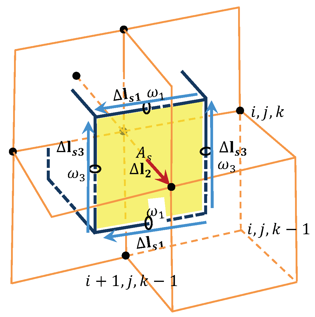
Employing staggered arrangement of variables, for component , we have:
2.2.2. Gaussian Divergence Theorem Applied to sst Model
The 3-D sst model was discretized numerically based on the FVM method. The FVM divides the domain into small control volumes, computes the fluxes of the conserved quantities across the boundaries of these volumes, and then updates the values within each volume based on these fluxes. A detailed derivation can be found in the appendix.
2.2.3. PARDISO Matrix Solver
After discretizing partial differential equations, the nonlinear equations transform into a set of linear equations, which can be solved using matrix solvers.
In numerical analysis, direct solvers like Gaussian elimination and LU decomposition are suitable for small to medium-sized problems. Indirect solvers, such as Jacobi iteration and the conjugate gradient method, are suited for large-scale problems with sparse matrices.
The matrices of the vorticity solver and the turbulence solver are solved by employing PARDISO (PARallel DIrect SOlver), an Intel-developed direct solver specifically designed for large sparse linear systems. It utilizes the multifrontal method that partitions the matrix into smaller dense submatrices, which can be solved more efficiently using a direct solver.
The parameters employed in PARDISO are detailed in Table 1. PARDISO begins with matrix analysis to establish the structure and sparsity pattern of the problem. Subsequent matrix reordering reduces fill-in and optimizes the sparsity structure, enhancing the efficiency of the factorization phase. PARDISO employs direct LU factorization methods. This process uses pivoting strategies to handle ill-conditioned matrices. After factorization, PARDISO efficiently solves the linear system for multiple right-hand sides and may employ iterative refinement for higher solution accuracy. Please note that only a subset of these parameters is listed, with the unmentioned parameters using their default values. For more detail, refer to the user guide [38].
2.2.4. Parallelization
Parallelizing numerical simulations is crucial when incorporating turbulence effects into models due to the time demands of simulating turbulent flows.
In order to achieve optimal performance on multi-core and multi-processor systems, it is crucial to fully utilize the features of parallelism and efficiently manage the memory hierarchy.
MPI (Message Passing Interface) applications can facilitate scalability across multiple SMP (Symmetric Multiprocessing) nodes. OpenMP applications can improve the efficient utilization of shared memory on SMP nodes. By incorporating MPI and OpenMP during the coding process, efficiency, performance, and scaling can be maximized. Hybridization refers to a method of employing different parallelization models to leverage the advantages of each.
2.2.5. A Summary of the Numerical Model for 3-D Turbulent Flow
Figure 2 provides a summary of the numerical models employed in the VISVE method for 3D turbulent flow simulations. The figure outlines the sequential steps involved in the simulation process:
- Initialization Procedure: The simulation starts with an initialization procedure for both vorticity and velocity fields. This step sets the initial conditions for the fluid flow simulation.
- Poisson Solver: The Poisson solver is used to compute the velocity field based on the initial vorticity and velocity distributions. It solves the Poisson equation to obtain the velocity field.
- Turbulence Solver: The turbulence solver then takes the velocity field obtained from the Poisson solver and calculates the turbulent viscosity within the flow domain.
- Turbulent VISVE solver: Turbulent viscosity is considered in addition to the molecular viscosity, allowing the model to capture the effects of turbulence more accurately. Using the computed turbulent viscosity, the turbulent VISVE solver updates the overall viscosity of the fluid.
- BEM Solver: A Boundary Element Method (BEM) solver is applied to correct the vorticity distribution at the boundary to satisfy the boundary conditions. Additionally, the BEM solver includes "images" to account for infinite geometries like hydrofoils, hubs, and other blades in the flow domain.
3. Application and Results
Turbulence is not a feature of fluids but of fluid flows. Since the equations of motion are nonlinear, each individual flow pattern has certain unique characteristics that are associated with its initial and boundary conditions. No general solutions are available to turbulent flows. The characteristics of turbulence depend on its environment. Because of this, turbulence theory does not attempt to deal with all kinds and types of flows in a general way. Similarly, the developed numerical model should be applied to specific scenarios.
In this section, the 3-D wing is characterized by its maximum chord length c. The Reynolds number, Re = , is defined in terms of the density of the fluid , the inflow velocity , the chord length of the hydrofoil c, and the dynamic viscosity of the fluid . The time step size used in this section is = 0.0001 s.
3.1. Geometry of the Rectangular Wing
A rectangular wing featuring a NACA (National Advisory Committee for Aeronautics) 4-digit section profile is utilized to perform testing on the newly developed model. The 4-digit designation refers to a specific series of numbers that determine the airfoil’s shape, thickness, and camber. As illustrated in Figure 3, the wing has a rectangular planform with a specified length as 1m and width as 1m. It has a constant chord length c as 1 m and a closed tip. The section with the maximum thickness is located at y = 0 along the span, where it has a NACA0008 profile. The first two digits represent the camber line of the airfoil. In the case of "00", it suggests a symmetric foil. The last two digits denote the thickness-to-chord ratio of the foil at a particular location along the chord. For "08", the thickness is 8% at 30% of the chord length. Moving towards the wingtip, the thickness of the other sections decreases linearly until it reaches zero.
As shown in Figure 3, the foil is discretized in the spanwise direction using a cosine spacing. Cosine spacing can concentrate more grid points in areas of higher curvature or significant flow variations, such as the leading and trailing edges. It allocates fewer points to regions with lower curvature or relatively uniform flow, optimizing grid resolution for computational efficiency.
The wing is aligned with a specified periodic direction, indicating that flow and other characteristics on one side mirror those on the opposite side. Figure 4 illustrates this by depicting half of the wing with the NACA 4-digit section profile. The periodic boundary condition presumes the existence of the complementary wing half, introducing virtual symmetry in the flow. The total width of the wing is equal to twice the chord length. The flow domain of the image and that of the key foil are symmetric with respect to the plane y = 0.
3.2. Computational Settings
3.2.1. Computational Settings in VISVE
The mesh of the wing is shown in Figure 5. The grid is comprised of sixteen blocks, which are highlighted in sixteen different colors. The normal height of the grid is only 20% of the chord length, and the length of the wake region is about 20% of the chord length. A total number of 306,176 cells were used in the mesh. The results obtained from the current method are presented together with those from RANS simulations.
In this case, the Reynolds number Re is 4 , with incoming velocity being 4.0 m/s and the molecular kinematic viscosity being s−1.
3.2.2. Computational Settings in RANS
Ansys-Fluent (Release 20.2) was used to conduct the RANS simulations. The size of the RANS domain is given in Figure 6. Overall, about 3 million hexahedral cells were used to discretize the RANS computational domain.
The computational domain used in a RANS simulation needs to be sufficiently large. External flows often require substantial domain size to accommodate appropriate inflow and outflow conditions. A larger domain helps to minimize the impact of boundary effects on the region of interest. Typically, a recommended practice is to have a computational domain that extends at least five times the characteristic length of the object upstream and ten times downstream.
Table 2 summarizes the key computational settings implemented in Fluent for the study. The solver is configured for pressure-based, segregated flow, utilizing the k- SST turbulence model. A second-order upwind numerical scheme is adopted, and the pressure-velocity coupling is managed through the SIMPLE algorithm. The time step is set at seconds, with a stringent convergence criterion of residuals less than . Initialization is performed from the inlet, and the boundary conditions include velocity inlet, pressure outlet, non-slip at the wall, and symmetry at midchord. The mesh is structured, and manual grid refinement is applied. These settings form the foundation of the computational model for the subsequent simulations.
In Figure 6, a comparison is presented between the computational domains of the VISVE and RANS solvers. The red mesh represents the domain utilized by VISVE, while the black domain corresponds to the RANS calculations. Notably, the VISVE domain is significantly more compact in contrast to the RANS domain. The expansiveness of the RANS domain is necessary to address the requirements of external flow problems. Conversely, VISVE exhibits a more localized influence, with vorticity concentrated in a small region near the wall.
Table 3 illustrates a comparison on the number of grids and the computational time required per iteration between the VISVE and RANS models. With 40 CPUs allocated to both cases, the VISVE method exhibits four times the speed of the RANS method.
3.3. Convergence Test
Convergence testing is an essential step in computational fluid dynamics (CFD), monitoring the convergence behavior of key solution variables to ensure that they approach a stable and consistent solution. Convergence testing typically involves varying certain parameters, such as the grid resolution or time step size, and observing the convergence of solution variables of interest.
The simulation is first run with a coarse grid or a relatively large time step to obtain an initial solution. Then, the parameters are systematically refined or adjusted, and the simulation is rerun with each refinement.
Table 4 presents data related to the grids used in the convergence test for the wing case. It includes the corresponding grid numbers in the x, y, and z directions on the wing, as well as the total number of grids for each configuration. Each row represents a specific grid configuration.
Table 5 provides an overview of the different time step sizes used in the convergence test for the wing case.
Figure 7 and Figure 8 display the results of the grid convergence test for velocity profiles in different chordwise and spanwise directions. The results of the convergence test indicate that Grid 4 and 5 diverged from the other grids, and time step = 0.0002 s also diverged from the other time steps. Those data did not converge as expected compared to the rest of the grids and time steps. Other meshes and time steps are converged well.
Therefore, it is recommended to use grid sizes greater than 20 in the spanwise direction, while a grid size of 64 is considered a suitable choice for the x direction. Additionally, both grid sizes of 30 and 46 work well in the z direction. A time step no greater than = 0.0001s is recommended.
In addition to the grid resolution around the hydrofoil, convergence tests are also conducted for the wake length. The wake region is a critical area when studying flow around hydrofoils. The flow in the wake region is often complex and can significantly impact the overall flow patterns, pressure distribution, and forces acting on the hydrofoil.
Figure 9 shows a comparison of two different computational domains used in the convergence tests. The long wake configuration shows a wake region that extends 2 meters behind the hydrofoil, while the short wake configuration shows a wake region of only 0.2 meters in length.
Figure 10, Figure 11, Figure 12, Figure 13 and Figure 14 shows the comparisons of velocity and vorticity, between the long wake and short wake configurations. The main objective of using an AOA of 0 degrees was to investigate the convergence behavior in a symmetric flow scenario. The symmetric flow condition serves as a reference case, allowing to focus on the influence of wake length on the convergence behavior. The observed convergence for different wake lengths in the symmetric flow suggests that the simulation results are grid-independent for the range of wake lengths tested.
Investigating the convergence test with respect to different wake lengths while considering the Angle Of Attack (AOA) is of significant importance. The AOA plays a crucial role in altering the behavior of vorticity, resulting in asymmetric flow patterns. Figure 15, Figure 16, Figure 17, Figure 18 and Figure 19 present velocity and vorticity profiles at different boundary layer locations, while maintaining a constant Angle Of Attack (AOA) as 2 degrees. The numerical solutions remain relatively consistent and independent of the specific length of the wake in this particular study. It enables the identification of the optimal grid resolution needed to capture the wake length and AOA effects accurately. One can use a short wake configuration in this case to increase computational speed while performing numerical simulations.
Figure 15.
Grid convergence test with respect to different length of wake, x/c = 0.2, y/c = 0.5, AOA = , Re = .
Figure 15.
Grid convergence test with respect to different length of wake, x/c = 0.2, y/c = 0.5, AOA = , Re = .
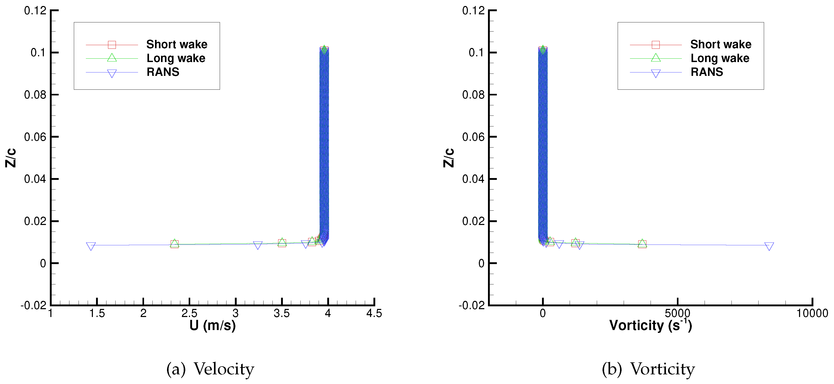
Figure 16.
Grid convergence test with respect to different length of wake, x/c = 0.5, y/c = 0.5, AOA = , Re = .
Figure 16.
Grid convergence test with respect to different length of wake, x/c = 0.5, y/c = 0.5, AOA = , Re = .
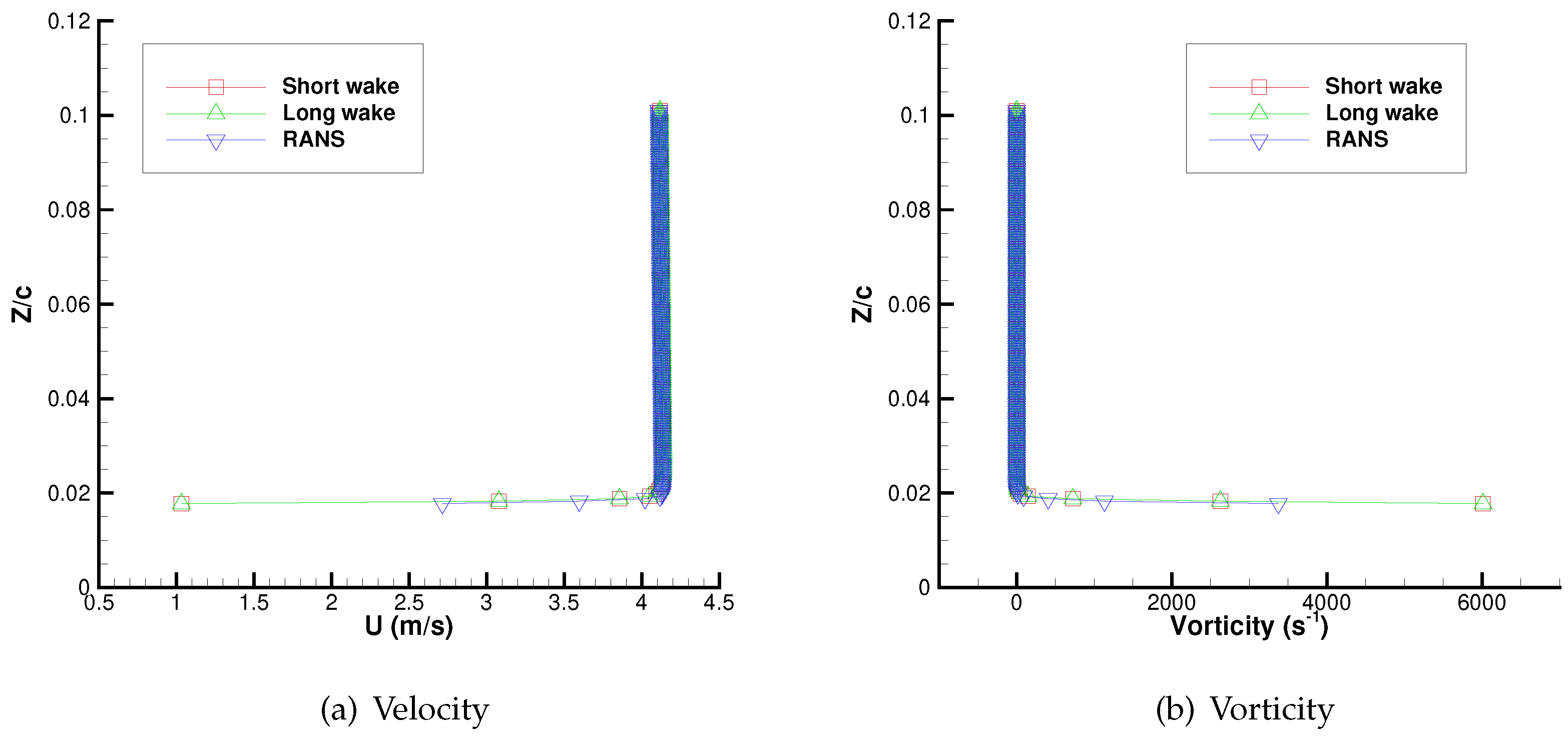
Figure 17.
Grid convergence test with respect to different length of wake, x/c = 0.8, y/c = 0.5, AOA = , Re = .
Figure 17.
Grid convergence test with respect to different length of wake, x/c = 0.8, y/c = 0.5, AOA = , Re = .
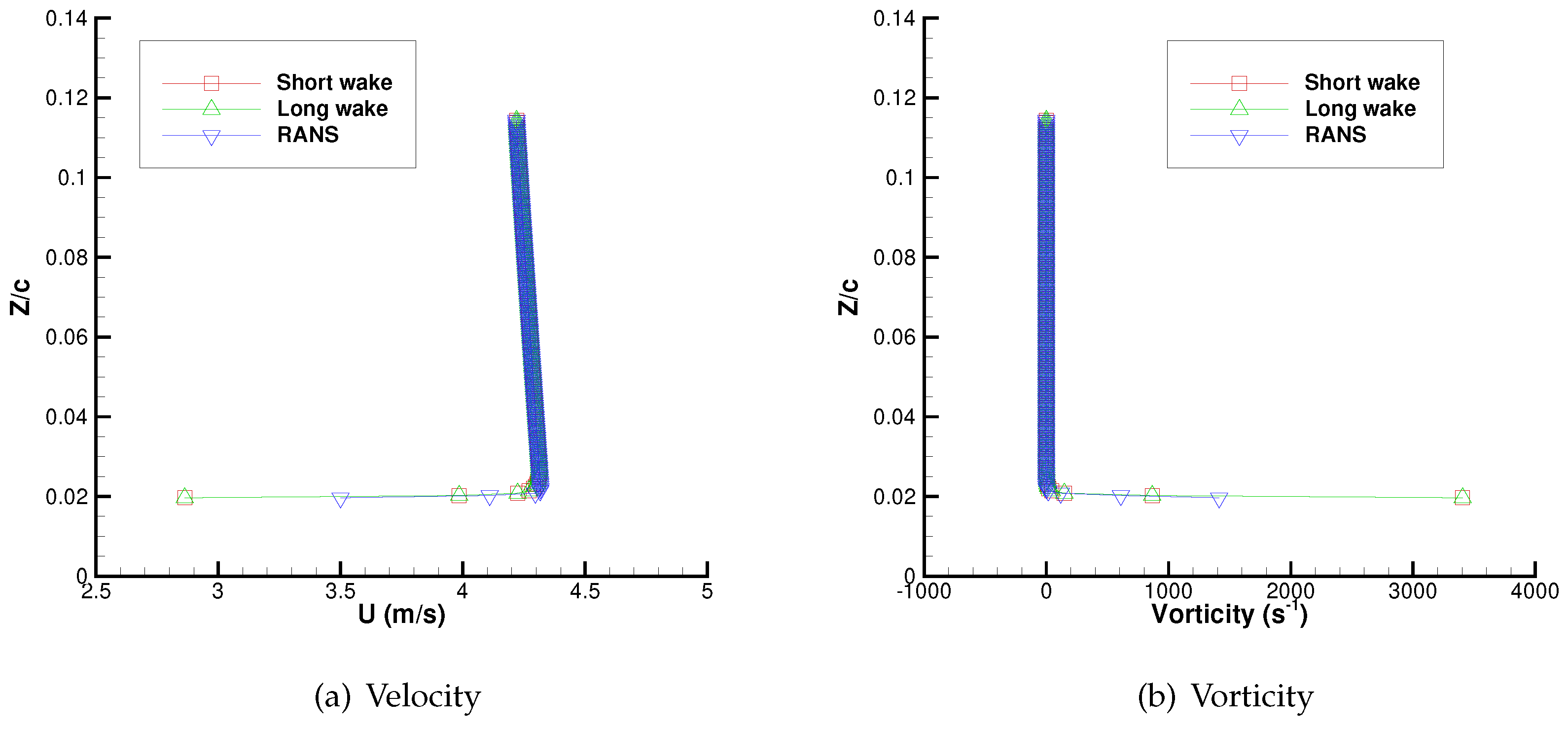
Figure 18.
Grid convergence test with respect to different length of wake, x/c = 0.5, y/c = 0.2, AOA = , Re = .
Figure 18.
Grid convergence test with respect to different length of wake, x/c = 0.5, y/c = 0.2, AOA = , Re = .
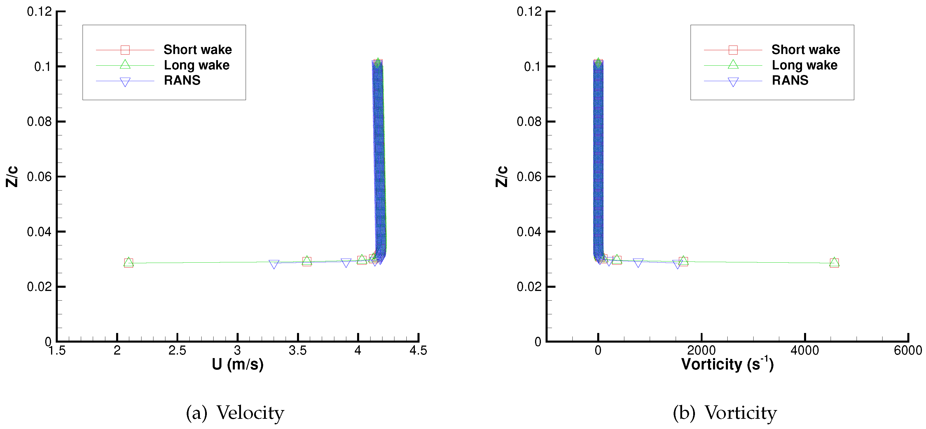
Figure 19.
Grid convergence test with respect to different length of wake, x/c = 0.5, y/c = 0.8, AOA = , Re = .
Figure 19.
Grid convergence test with respect to different length of wake, x/c = 0.5, y/c = 0.8, AOA = , Re = .
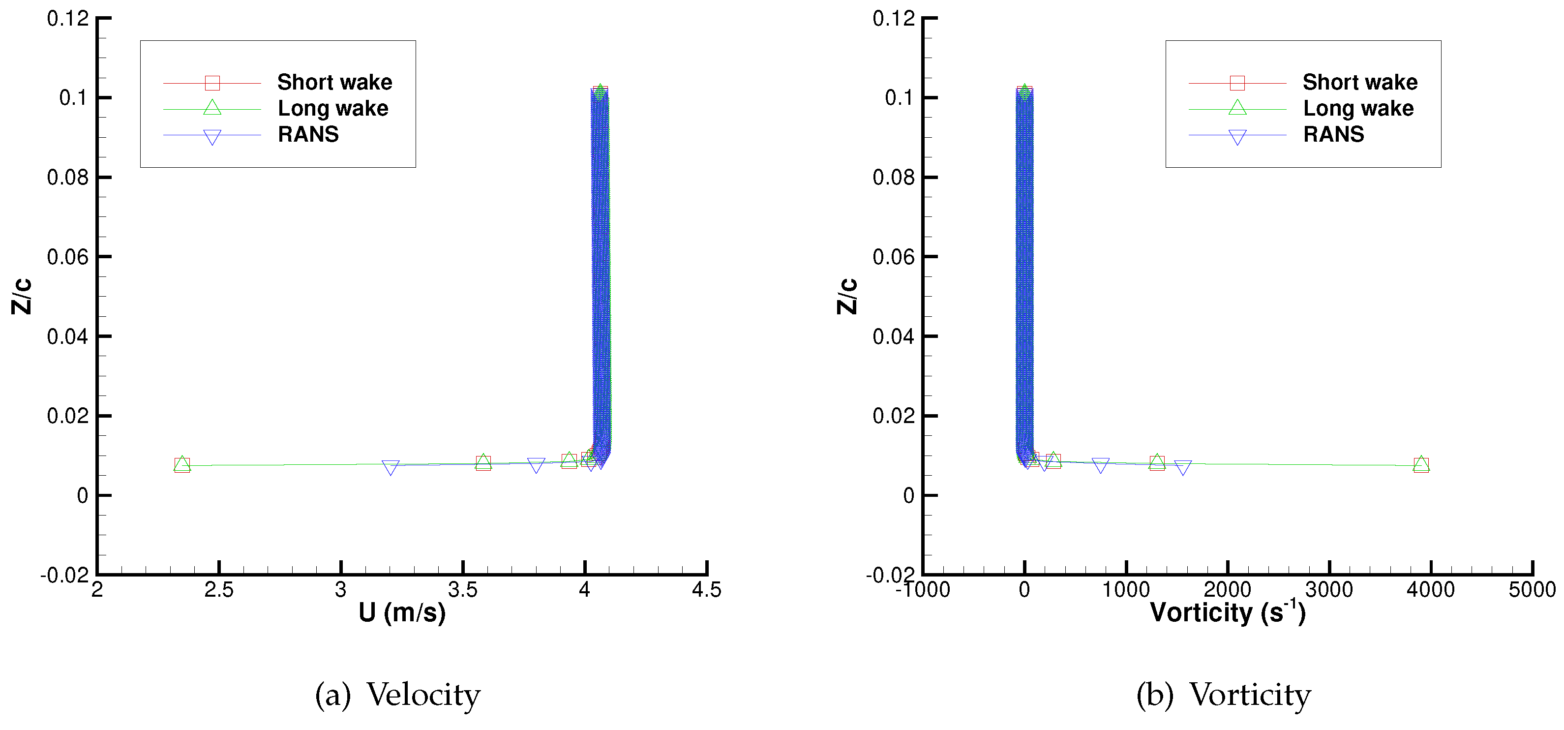
Figure 20.
Time step convergence test for velocity profiles in different chordwise directions, y/c = 0.2, AOA = , Re = .
Figure 20.
Time step convergence test for velocity profiles in different chordwise directions, y/c = 0.2, AOA = , Re = .
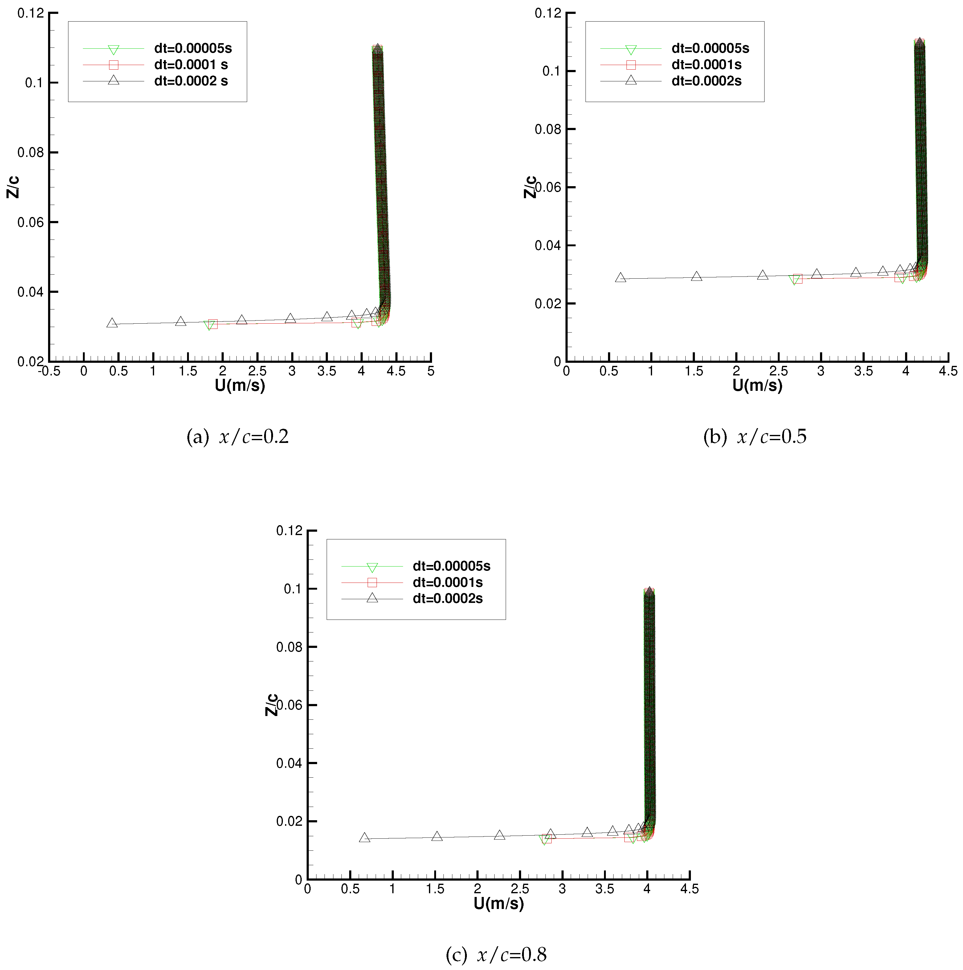
Figure 21.
Time step convergence test for velocity profiles in different spanwise directions, x/c = 0.5, AOA = , Re = .
Figure 21.
Time step convergence test for velocity profiles in different spanwise directions, x/c = 0.5, AOA = , Re = .
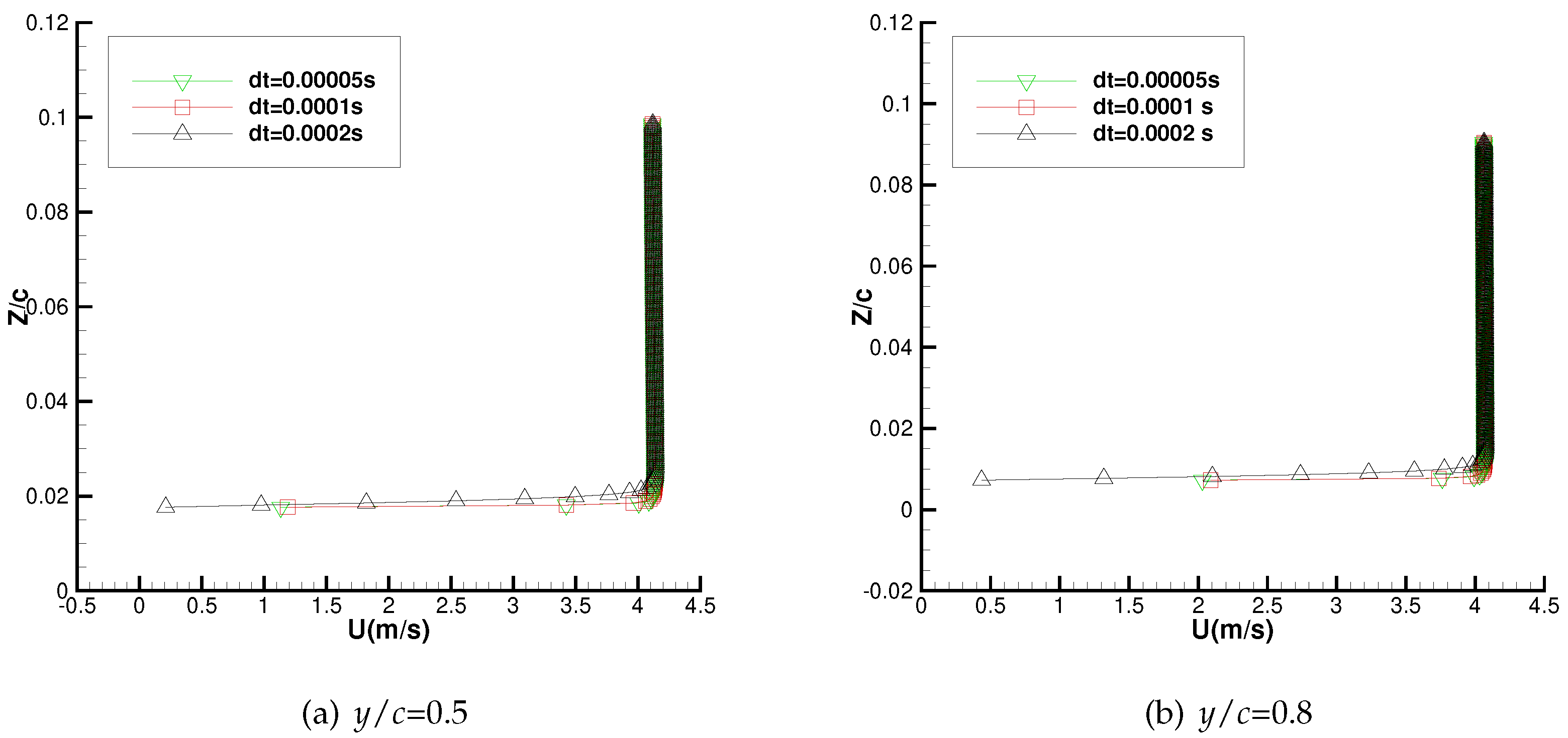
3.4. Comparison between VISVE and RANS Results
In this section, computational experiments will be conducted at two different angles of attack. This analysis involves examining a symmetric flow at a 0-degree angle of attack and an asymmetric flow with a 2-degree angle of attack (AOA). While the cases are designed to be steady, they will be simulated in an unsteady manner, gradually converging to a steady state. The results obtained during both the unsteady and steady states will be compared. Comprehensive qualitative and quantitative comparisons will be executed, entailing a detailed assessment of contours and profiles in relation to results obtained from the RANS solver. Various properties, including vorticity, velocity, and pressure, will be scrutinized through a comparative analysis.
3.4.1. Unsteady State
By comparing the VISVE results with RANS results taken at different time instances, one can evaluate how well the VISVE model predicts the changes in flow behavior over time. It provides insight into the ability of the simulation to capture the dynamic nature of the fluid flow. It also serves as preliminary investigation for time-dependent phenomena such as vortex shedding, oscillations, or transitional behaviors.
The results obtained from the current method are presented together with those from RANS simulations. Figure 22 shows the comparisons of velocity contour between 3-D turbulent VISVE and RANS at different span-wise cross-sections. Figure 23 presents the comparison of velocity profiles between VISVE and RANS at zero angle of attack. Figure 24 shows a similar comparison as in Figure 23, but have an unsymmetrical flow with an AOA = .
3.4.2. Steady State
Figure 25 and Figure 26 depict the comparison of velocity and vorticity contours between the 3-D Turbulent VISVE method and RANS simulations. Five spanwise locations are examined, ranging from = 0.1 to 0.9 towards the tip. Despite the different underlying principles and computational approaches, the two methods yield comparable predictions of the flow characteristics. The similarity between RANS and VISVE suggests that the 3-D Turbulent VISVE method is capable of accurately capturing the flow features. By examining multiple spanwise locations, the study provides a comprehensive analysis of the agreement between RANS and VISVE simulations. The consistency observed across different spanwise locations enhances the confidence in the accuracy and reliability of the 3-D Turbulent VISVE method.
Figure 27 and Figure 28 display the velocity and vorticity contours at AOA=. An angle of attack (AOA) is the angle between the chord line of a foil and the oncoming flow direction. The AOA affects the formation and structure of vortices and the wake behind the hydrofoil.
Figure 27.
Comparison of the velocity contours between 3-D Turbulent VISVE and RANS. Re= , AOA=.
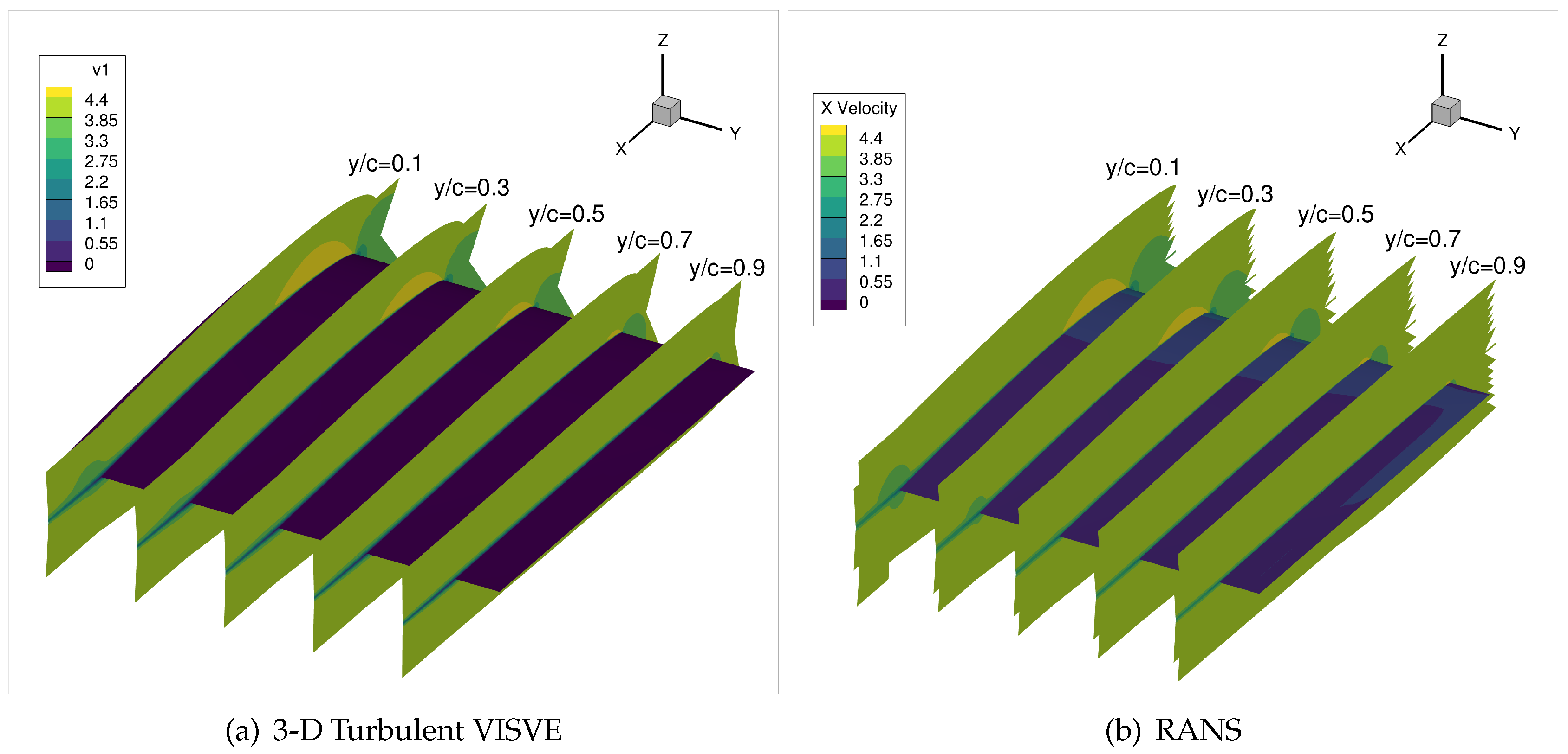
Figure 28.
Comparison of the vorticity contours between 3-D Turbulent VISVE and RANS. Re= , AOA=.
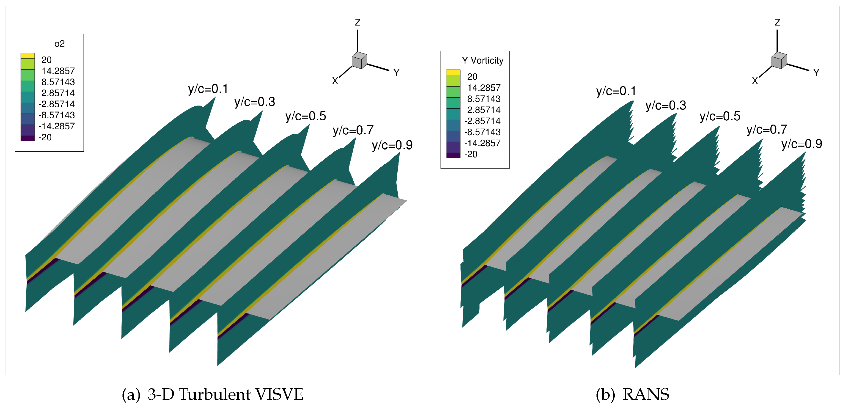
Figure 29.
Velocity profiles at different spanwise direction y/c=0.3, 0.5, 0.7. Re=, AOA=.
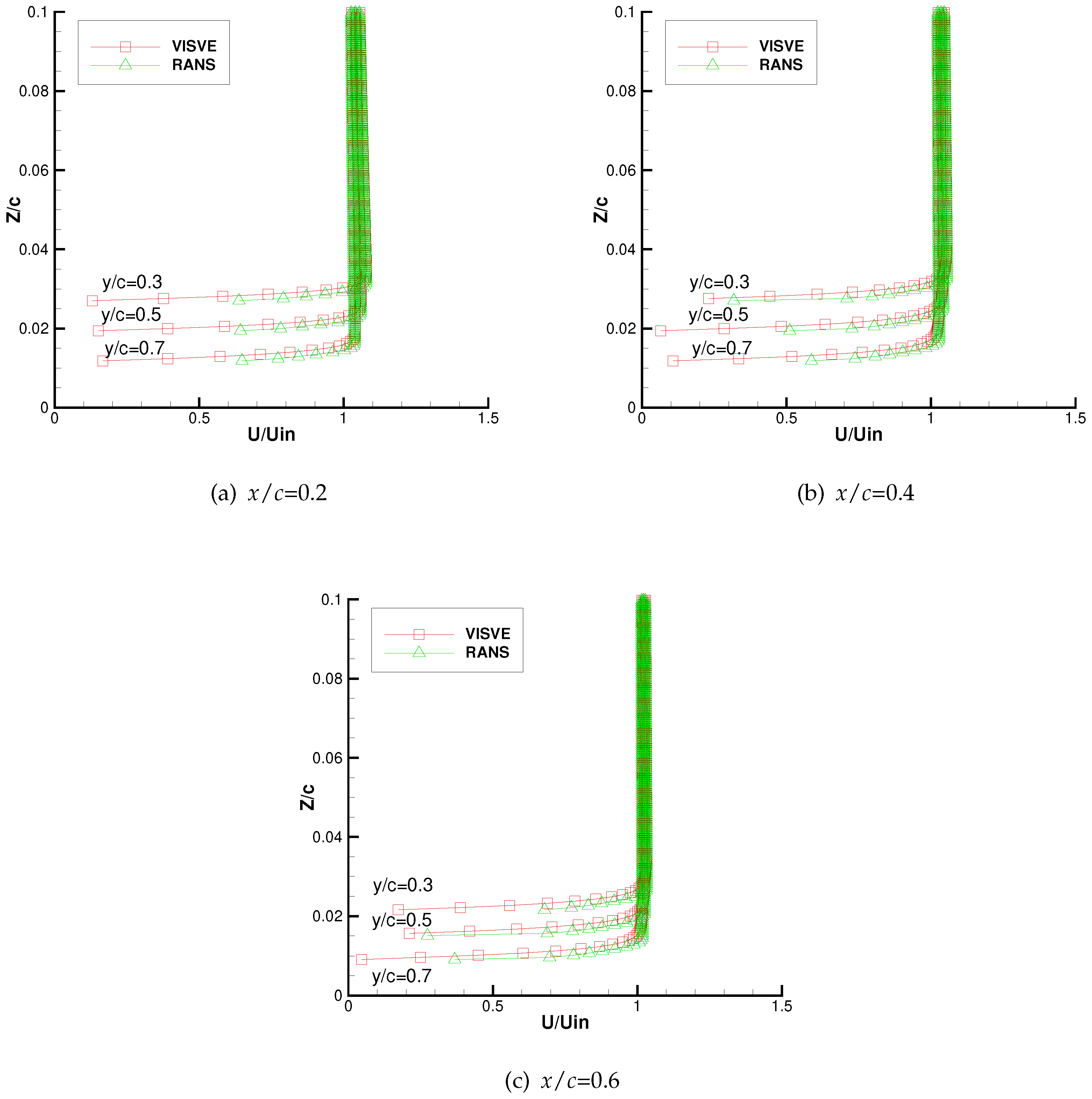
Figure 30.
Vorticity profiles at different spanwise direction y/c=0.3, 0.5, 0.7. Re=, AOA=.
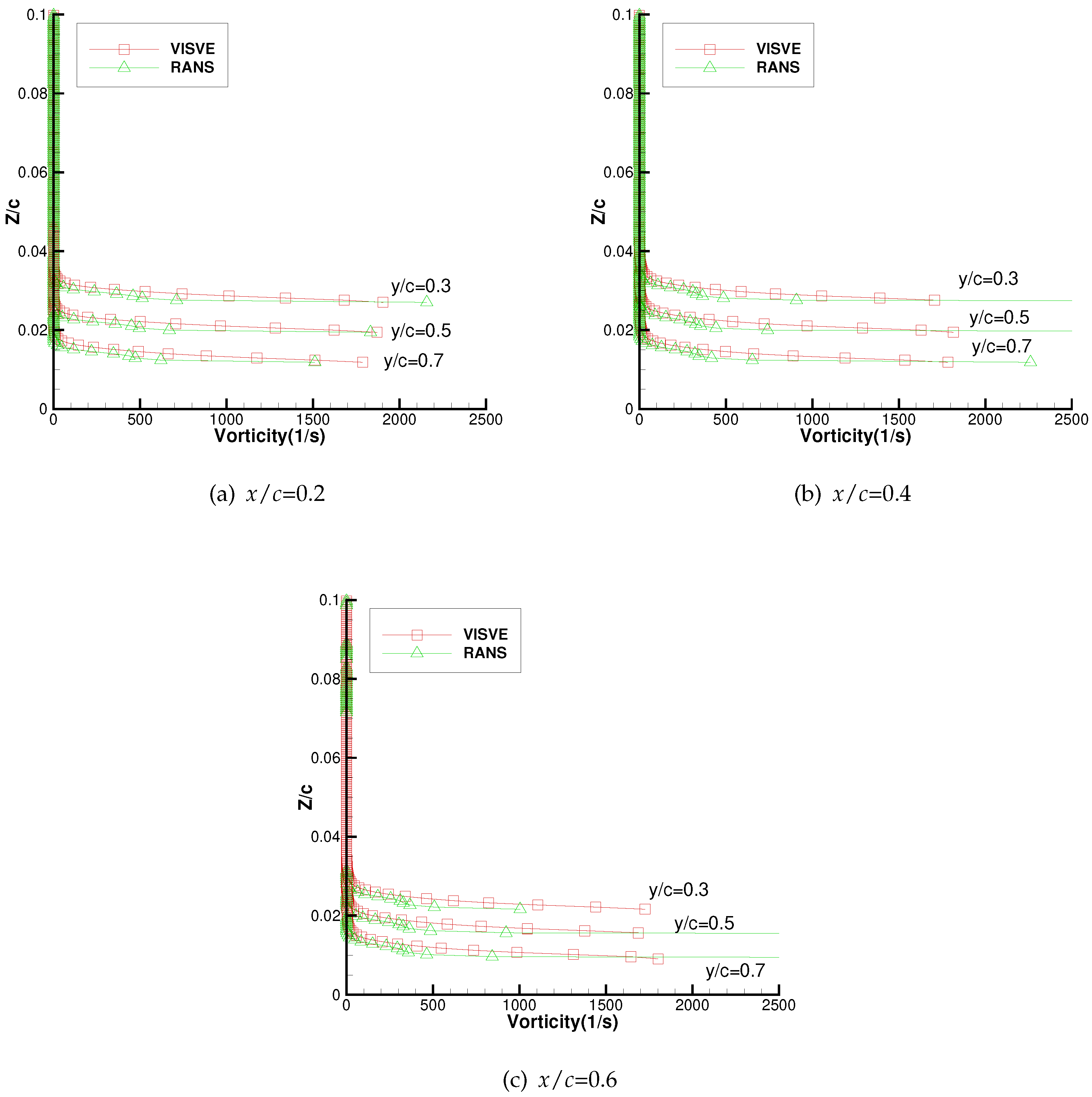
Figure 31.
Velocity profiles at different spanwise direction y/c=0.3, 0.5, 0.7. Re=, AOA=.
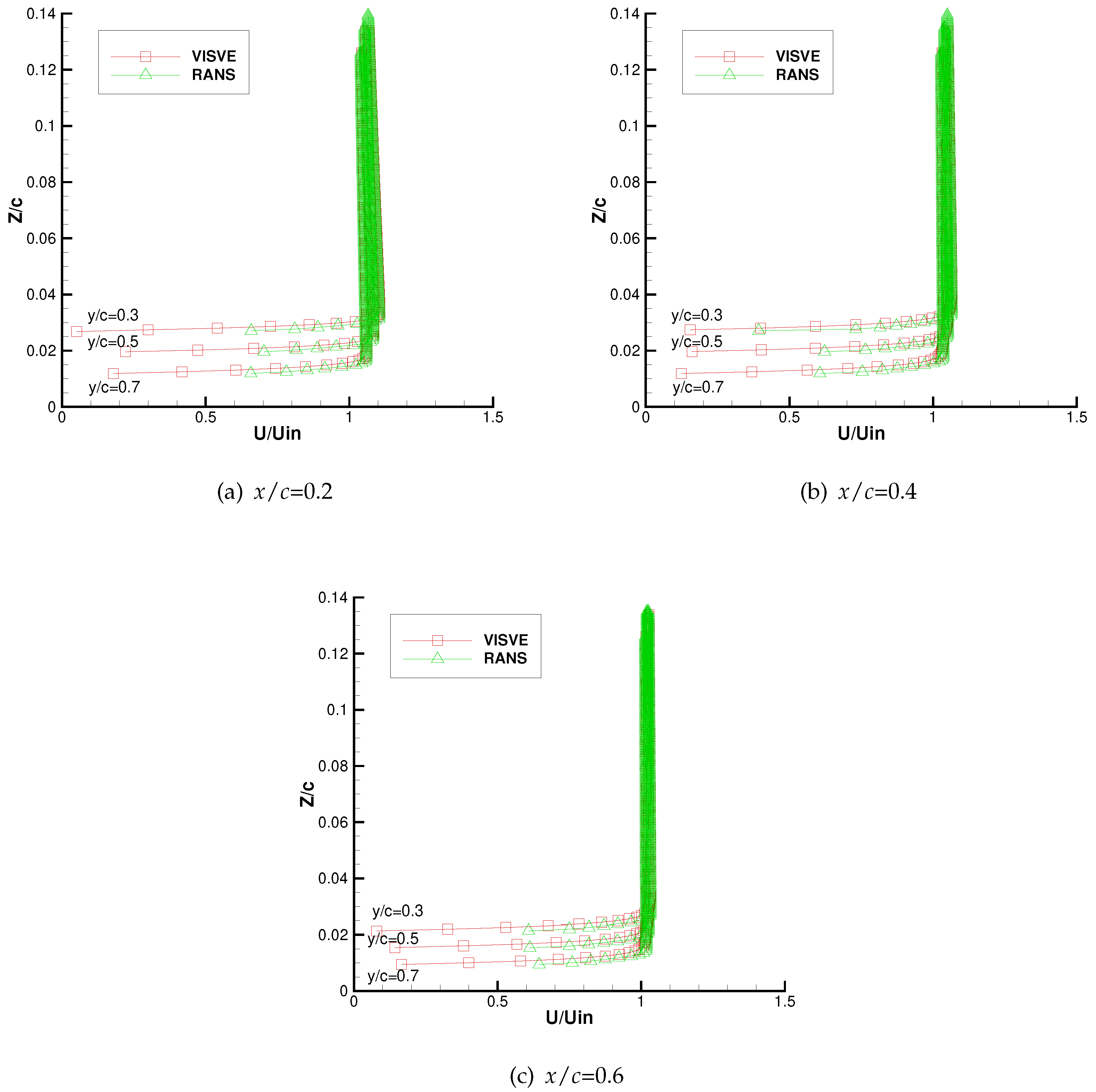
Figure 32.
Vorticity profiles at different spanwise direction y/c=0.3, 0.5, 0.7. Re=, AOA=.
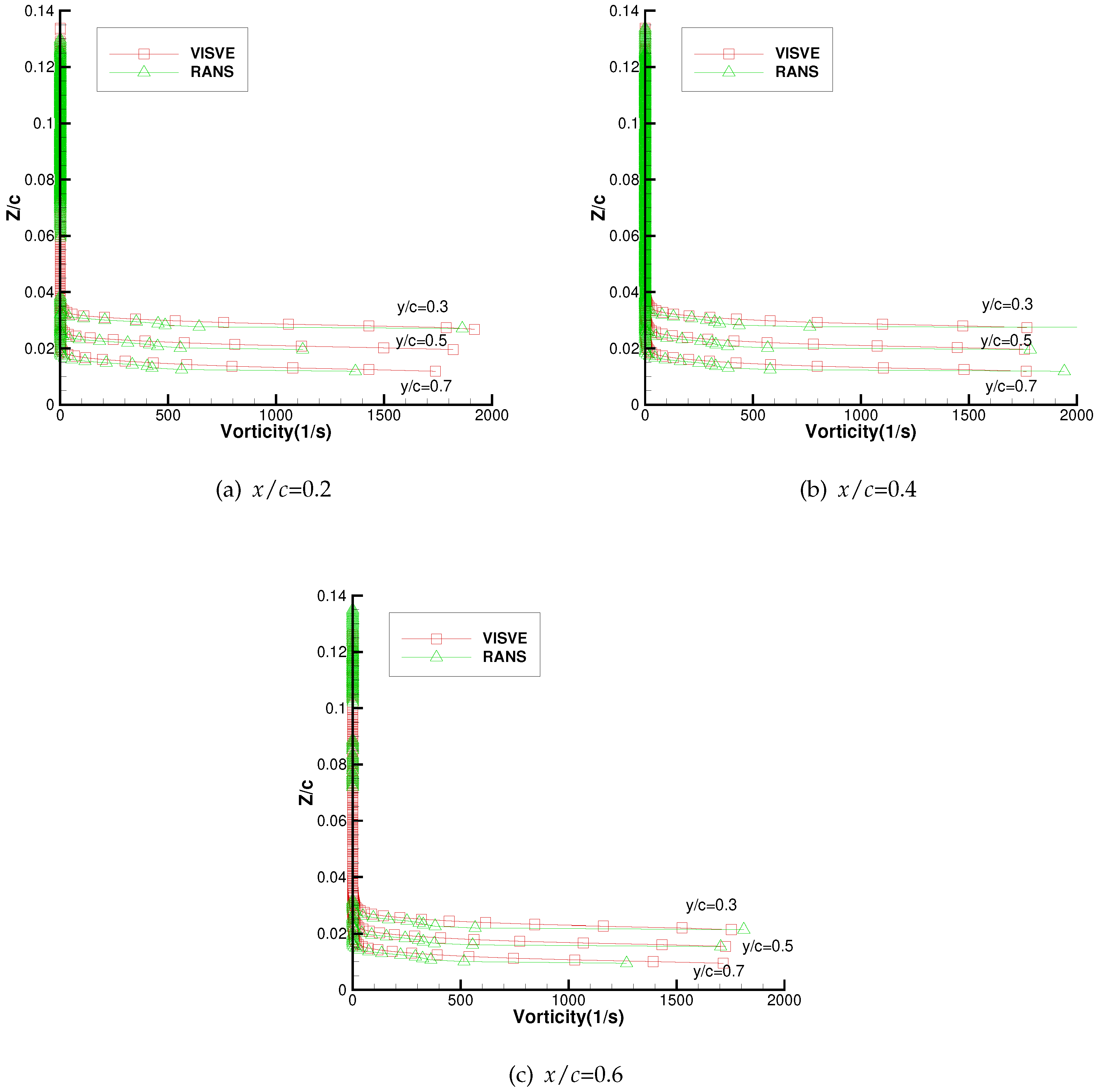
Once fluid properties like velocity and vorticity are assessed in a steady state, attention turns to exploring hydrodynamics. Figure 33 displays pressure distribution on the wing across various spanwise sections. Agreement with RANS is noted at most chordwise and spanwise positions, except in the vicinity of the leading edge. Differences at the leading edge when predicting pressure can arise due to several reasons. Future investigation will be carried on the velocity of the leading edge.
4. Conclusions
The research successfully developed an efficient numerical solver, based on the 3-D VIScous Vorticity Equation (VISVE) model, capable of simulating turbulent flows around hydrofoils. This study implemented the SST turbulence model within the 3-D VISVE solver, extending its applicability to turbulent flow scenarios. The adoption of a hybrid OpenMP/MPI parallelization strategy allowed for the efficient utilization of High-Performance Computing (HPC) resources, enhancing the solver’s computational efficiency. The conducted convergence tests and the analysis of a 3-D hydrofoil showcased the solver’s consistency with results obtained from a Reynolds-Averaged Navier-Stokes (RANS) solver, highlighting its accuracy and reliability in turbulent flow simulations. The research showcased significant reductions in computational domain, unknowns, and computation time for the hydrofoil case.
Overall, this research contributes to the development of a robust and efficient numerical solver for simulating turbulent flows around hydrofoils. Having successfully assessed the stability and reliability of the presented developed 3-D turbulent VISVE solver, the subsequent phase includes an examination of the rotational turbulent flow and the practical application to a rotational propeller.
Author Contributions
Methodology, software, validation, investigation, data curation, writing—original draft preparation, Rui You; conceptualization, funding acquisition, supervision, project administration, writing—review and editing, Spyros A. Kinnas. All authors have read and agreed to the published version of the manuscript.
Funding
Support for this research was provided by the U.S. Office of Naval Research (Grant Numbers N00014-18-1-2276 and N00014-21-1-2488; Dr. Yin Lu Young) and by Phases VIII, and IX of the “Consortium on Cavitation Performance of High Speed Propulsors”.
Institutional Review Board Statement
Not applicable
Informed Consent Statement
Not applicable
Conflicts of Interest
The authors declare no conflict of interest.
Appendix A. Numerical implementation of the 3-D k-ω SST model
This appendix presents the newly developed 3-D turbulence model, highlighting the incorporation of turbulence effects.
To numerically solve the SST turbulence model, as described in Section 2.1.3, a Finite Volume Method (FVM) is employed. By applying the Gaussian divergence theorem, Equation (A1) is obtained.
Appendix A.1. Convective term
First, we examine the convective term.
The k value at the face can be represented by the k at the centroid:
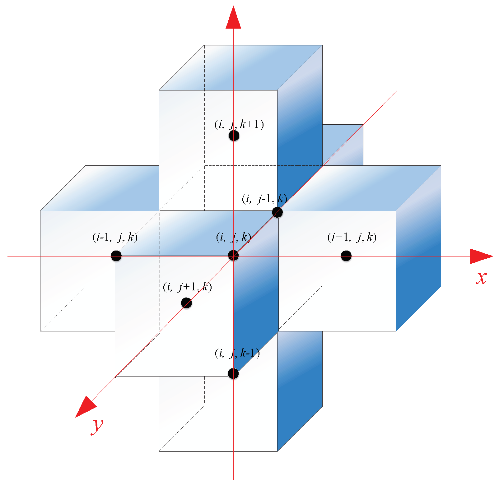
In Figure A1, the coordinates and indices are shown for the 3-D turbulence model after the process of discretization.
Figure A1.
Indices for the 3-D turbulence model
Appendix A.2. Diffusive term
The diffusive term can also be expressed as the sum of six faces over each control volume.
with
Equation (A5) can be written as:
Appendix A.3. Source term
When dealing with structured orthogonal grids, calculating the gradient of a scalar at a control volume centroid is straightforward using the definition of derivatives. However, for general unstructured grids, the process becomes more complex. In such cases, the Green-Gauss theorem is commonly used as a numerical method. This theorem relates the surface integral of a scalar function to the volume integral of the gradient of the scalar function.
The Green-Gauss method is employed for calculating gradients in Finite Volume Methods (FVM). It is considered an attractive method due to its adherence to the principles of FVM discretization for other partial differential terms. This method has been shown to outperform the least-squares (LS) gradient method in simulating aerodynamic boundary layer flows over curved surfaces, as analyzed by Syrakos et al. [39]. Additionally, the Green-Gauss method is not restricted algorithmically to a specific grid cell geometry and can be applied to cells with an arbitrary number of faces. This flexibility is particularly important as unstructured grids have become a standard practice in simulating complex engineering processes in recent years.
The rate of stain term in production:
where, the components of the are:
Appendix B. Vorticity Solver
This appendix demonstrates the integration of turbulent viscosity into the vorticity transport equation. For the vorticity solver, the modification due to turbulence effect mainly focus on the diffusive term. The convective term remains unchanged from the laminar case, and thus, it will be omitted here. For details on addressing the convective term, please refer to [27].
This is the vorticity equation for 3-D turbulent flow.
After applying Stokes’s theorem, we obtain the discretized form, taking for example:
The diffusive terms encompass the turbulent viscosity. Applying Stokes’s theorem once again to the diffusive term involves taking the curl off. The turbulent viscosity is located from the face centroid to the edges after this operation.
The discretized form for all of the terms would be:
where, .
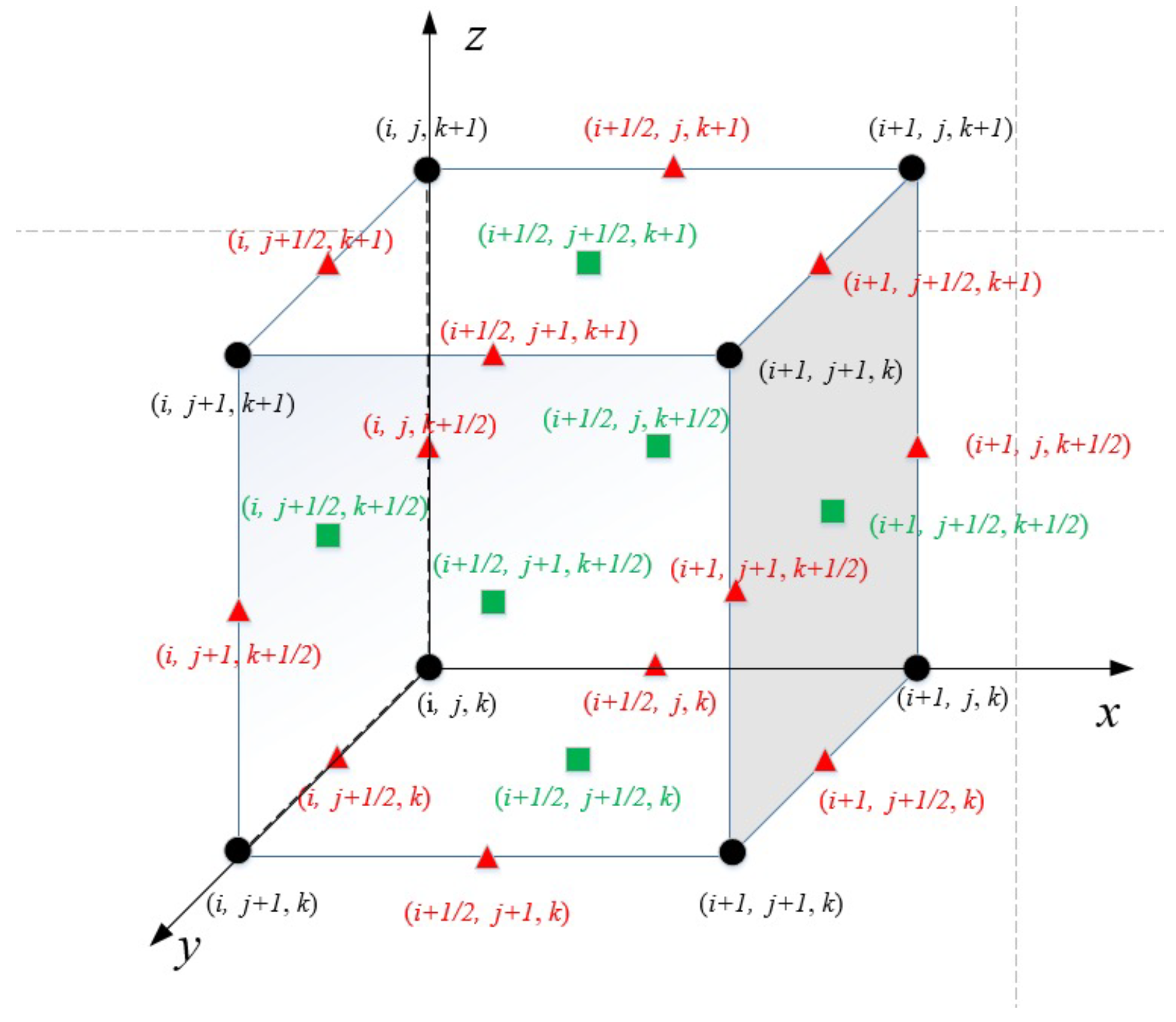
The turbulent viscosity calculated from the turbulence model is located at the centroid. To integrate it into the vorticity solver, interpolation from the centroid to the edges is required. Figure A2 illustrates the indexing scheme used for nodes, faces, and edges in a computational mesh.
Figure A2.
Index at nodes, faces and edges
Appendix C. Velocity Solver
This appendix illustrates how the vorticity-preserving velocity field is determined explicitly under turbulent flow.
Consider the requirement of ,
Handling the unsteady term with an explicit time method, we can obtain:
and
Equation (A18) is explicit, because all the terms in the RHS are known once is known.
After solving , the Poisson equation for velocity can be solved via a Finite Volume Method (FVM). This part will not be presented here as it is the same as the laminar solver. For further details, please refer to [27].
References
- Kerwin, J.E.; Lee, C.S. Prediction of steady and unsteady marine propeller performance by numerical lifting-surface theory. Technical report, 1978.
- Lee, C.S. Predicton of steady and unsteady performance of marine propellers with or without cavitation by numerical lifting-surface theory. PhD thesis, Massachusetts Institute of Technology, 1979.
- Kerwin, J.E. Marine propellers. Annual review of fluid mechanics 1986, 18, 367–403. [Google Scholar] [CrossRef]
- Kinnas, S.A. Non-linear corrections to the linear theory for the prediction of the cavitating flow around hydrofoils. PhD thesis, Massachusetts Institute of Technology, 1985.
- Kinnas, S.A. Leading-edge corrections to the linear theory of partially cavitating hydrofoils. Journal of Ship Research 1991, 35, 15–27. [Google Scholar] [CrossRef]
- Kinnas, S.A.; Fine, N.E. Theoretical prediction of midchord and face unsteady propeller sheet cavitation. International conference on numerical ship hydrodynamics, 5th, 1989.
- Lee, H. Modeling of unsteady blade sheet and developed tip vortex cavitation. PhD thesis, The University of Texas at Austin, 2001.
- Hess, J.L.; Smith, A.M.O. Calculation of potential flow about arbitrary bodies. Progress in Aerospace Sciences 1967, 8, 1–138. [Google Scholar] [CrossRef]
- Fine, N.E.; Kinnas, S.A. A boundary element method for the analysis of the flow around 3-D cavitating hydrofoils. Journal of ship research 1993, 37, 213–224. [Google Scholar] [CrossRef]
- Young, Y.L.; Kinnas, S.A. A BEM for the prediction of unsteady midchord face and/or back propeller cavitation. J. Fluids Eng. 2001, 123, 311–319. [Google Scholar] [CrossRef]
- Young, Y.L.; Kinnas, S.A. Performance prediction of surface-piercing propellers. Journal of Ship Research 2004, 48, 288–304. [Google Scholar] [CrossRef]
- Young, Y.L.; Kinnas, S.A. Numerical modeling of supercavitating propeller flows. Journal of Ship Research 2003, 47, 48–62. [Google Scholar] [CrossRef]
- Lee, H.; Kinnas, S.A. Application of a boundary element method in the prediction of unsteady blade sheet and developed tip vortex cavitation on marine propellers. Journal of Ship Research 2004, 48, 15–30. [Google Scholar] [CrossRef]
- Lee, H.; Kinnas, S.A. Unsteady wake alignment for propellers in nonaxisymmetric flows. Journal of Ship Research 2005, 49, 176–190. [Google Scholar] [CrossRef]
- Jessup, S.D. An experimental investigation of viscous aspects of propeller blade flow; The Catholic University of America, 1989.
- Hufford, G.S.; Drela, M.; Kerwin, J.E. Viscous flow around marine propellers using boundary-layer strip theory. Journal of ship research 1994, 38, 52–62. [Google Scholar] [CrossRef]
- Sun, H.; Kinnas, S.A. Performance prediction of cavitating water-jet propulsors using a viscous/inviscid interactive method. SNAME Maritime Convention. OnePetro, 2008. [CrossRef]
- Kinnas, S.A.; Jeon, C.H.; Purohit, J.; Tian, Y. Prediction of the unsteady cavitating performance of ducted propellers subject to an inclined inflow. International symposium on marine propulsors SMP, 2013, Vol. 13.
- Fluent, A. 2022 User’s guide. Ansys inc 2022, 6, 552. [Google Scholar]
- Siemens, P. STAR-CCM+ User Guide, Version 13.04; Siemens PLM Software Inc.: Munich, Germany, 2019.
- Greenshields, C.J. others. OpenFOAM user guide. OpenFOAM Foundation Ltd, version 2015, 3, 47.
- Tian, Y.; Kinnas, S.A. A viscous vorticity method for propeller tip flows and leading edge vortex. Fourth international symposium on marine propulsors (smp15), Austin, Texas, USA, 2015.
- Tian, Y. Leading edge vortex modeling and its effect on propulsor performance. PhD thesis, Ocean Engineering Group, Dept. of Civil, Architectural and Environmental Engineering, UT Austin, 2014.
- Wu, C.; Kinnas, S.A.; Li, Z.; Wu, Y. A conservative viscous vorticity method for unsteady unidirectional and oscillatory flow past a circular cylinder. Ocean Engineering 2019, 191, 106504. [Google Scholar] [CrossRef]
- Wu, C.; Kinnas, S.A. A 3-D VIScous Vorticity Equation (VISVE) Method Applied to Flow Past a Hydrofoil of Elliptical Planform and a Propeller. Proceedings of the 6th International Symposium on Marine Propulsors, SMP19, Rome, Italy, 2019, pp. 26–30.
- Wu, C.; Kinnas, S.A. Flow past a rotating cylinder predicted by a compact Eulerian viscous vorticity method under non-inertial rotating frame. Ocean Engineering 2021, 230, 108882. [Google Scholar] [CrossRef]
- Wu, C.; Kinnas, S.A. Parallel implementation of a VIScous Vorticity Equation (VISVE) method in 3-D laminar flow. Journal of Computational Physics 2021, 426, 109912. [Google Scholar] [CrossRef]
- Xing, L. VISVE, a vorticity based model applied to 2-D hydrofoils in backing and cavitating conditions. Master’s thesis, Ocean Engineering Group, Dept. of Civil, Architectural and Environmental Engineering, UT Austin, 2018.
- Iliopoulos, K.; Kinnas, S.A. VISVE, a Vorticity Based Model Applied to 2-D Hydrofoils in Cavitating Conditions. Proceedings of the 11th International Symposium on Cavitation, CAV2021, May 10-13, 2021.
- Kinnas, S.A. VIScous Vorticity Equation (VISVE) for Turbulent 2-D Flows with Variable Density and Viscosity. Journal of Marine Science and Engineering 2020, 8, 191. [Google Scholar] [CrossRef]
- Yao, H.; Kinnas, S.A. Coupling Viscous Vorticity Equation (VISVE) Method with OpenFOAM to Predict Turbulent Flow around 2-D Hydrofoils and Cylinders. Proceedings of the Twenty-ninth (2019) International Ocean and Polar Engineering Conference, ISOPE, Hawaii, USA, 2019, pp. 3442–3451.
- Wu, C.; Kinnas, S.A. Laminar and Turbulent Flow Past a Hydrofoil Predicted by a Distributed Vorticity Method. International Conference on Offshore Mechanics and Arctic Engineering. American Society of Mechanical Engineers, 2020, Vol. 84409, p. V008T08A008. [CrossRef]
- You, R.; Kinnas, S.A. VIScous Vorticity Equation (VISVE) model applied to 2-D turbulent flow over hydrofoils. Ocean Engineering 2022, 256, 111416. [Google Scholar] [CrossRef]
- You, R.; Tiwari, A.S.; Kinnas, S.A. VIScous Vorticity Equation (VISVE) Model Applied to Oscillatory Turbulent Flow around a Cylinder. SNAME 27th Offshore Symposium. OnePetro, 2022. [CrossRef]
- Kinnas, S.A. VIScous Vorticity Equation (VISVE) for Turbulent 3-D Flows with Variable Density and Viscosity. Under preparation 2023. [Google Scholar] [CrossRef]
- Menter, F.R. Two-equation eddy-viscosity turbulence models for engineering applications. AIAA journal 1994, 32, 1598–1605. [Google Scholar] [CrossRef]
- Wilcox, D.C. Turbulence modeling for CFD; Vol. 2, DCW industries La Canada, CA, 1998.
- Schenk, O.; Gärtner, K. Solving unsymmetric sparse systems of linear equations with PARDISO. Future Generation Computer Systems 2004, 20, 475–487. [Google Scholar] [CrossRef]
- Syrakos, A.; Varchanis, S.; Dimakopoulos, Y.; Goulas, A.; Tsamopoulos, J. A critical analysis of some popular methods for the discretisation of the gradient operator in finite volume methods. Physics of Fluids 2017, 29, 127103. [Google Scholar] [CrossRef]
Figure 2.
A summary of the numerical models employed in VISVE for 3-D turbulent flow.
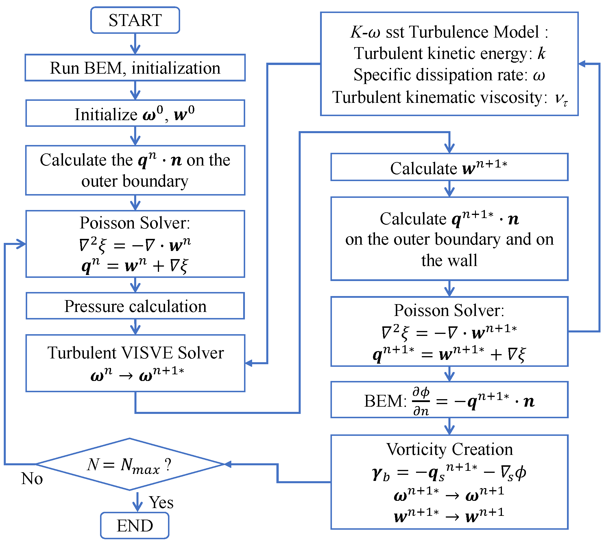
Figure 3.
The rectangular wing.
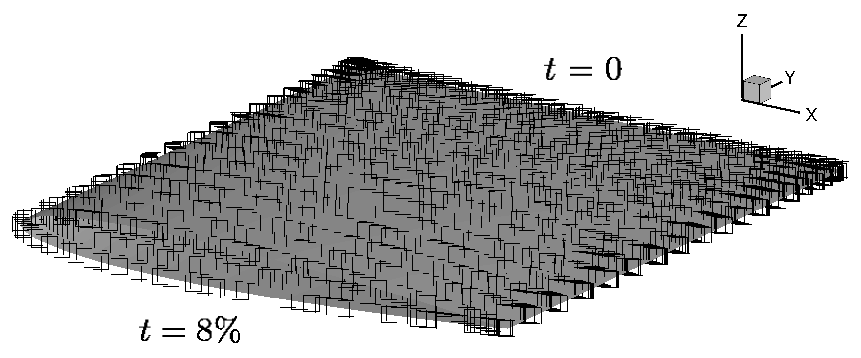
Figure 4.
The image model of a 3-D wing with one periodic direction.
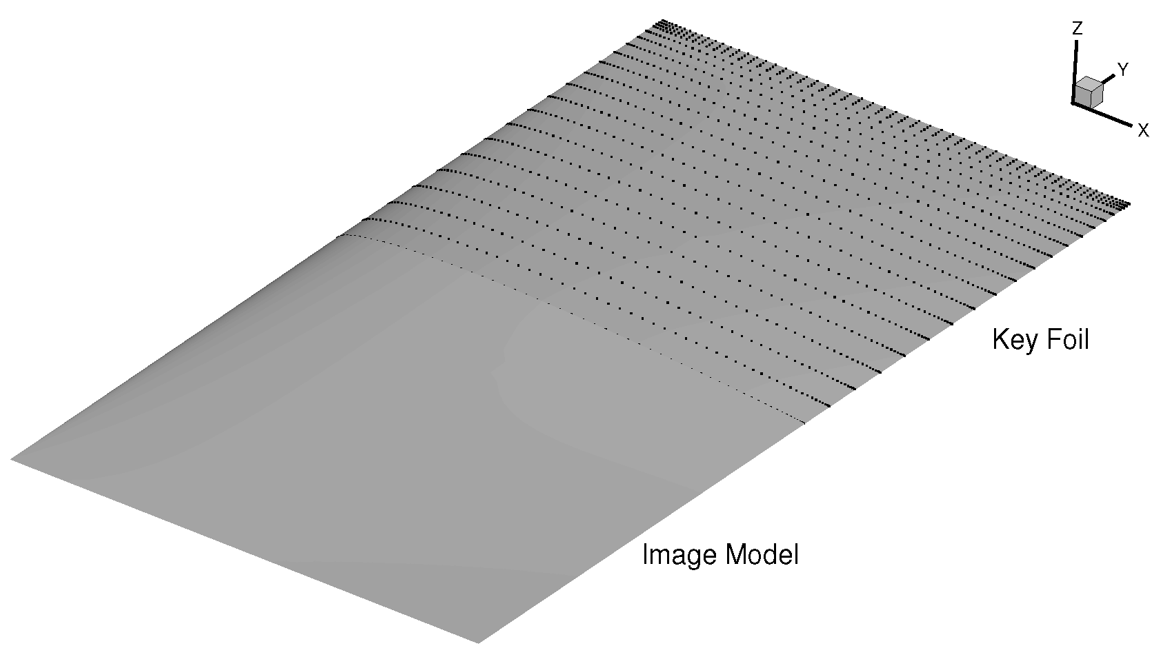
Figure 5.
The VISVE grid used for the flow past the rectangular wing.
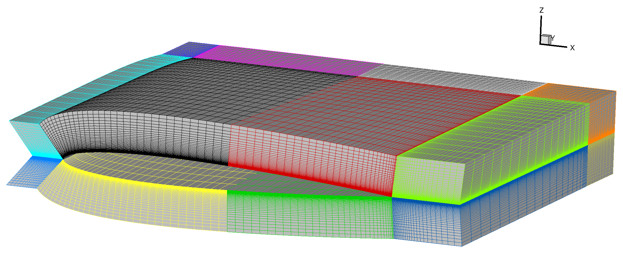
Figure 6.
Comparison of the computational domains between VISVE and RANS for the rectangular wing.
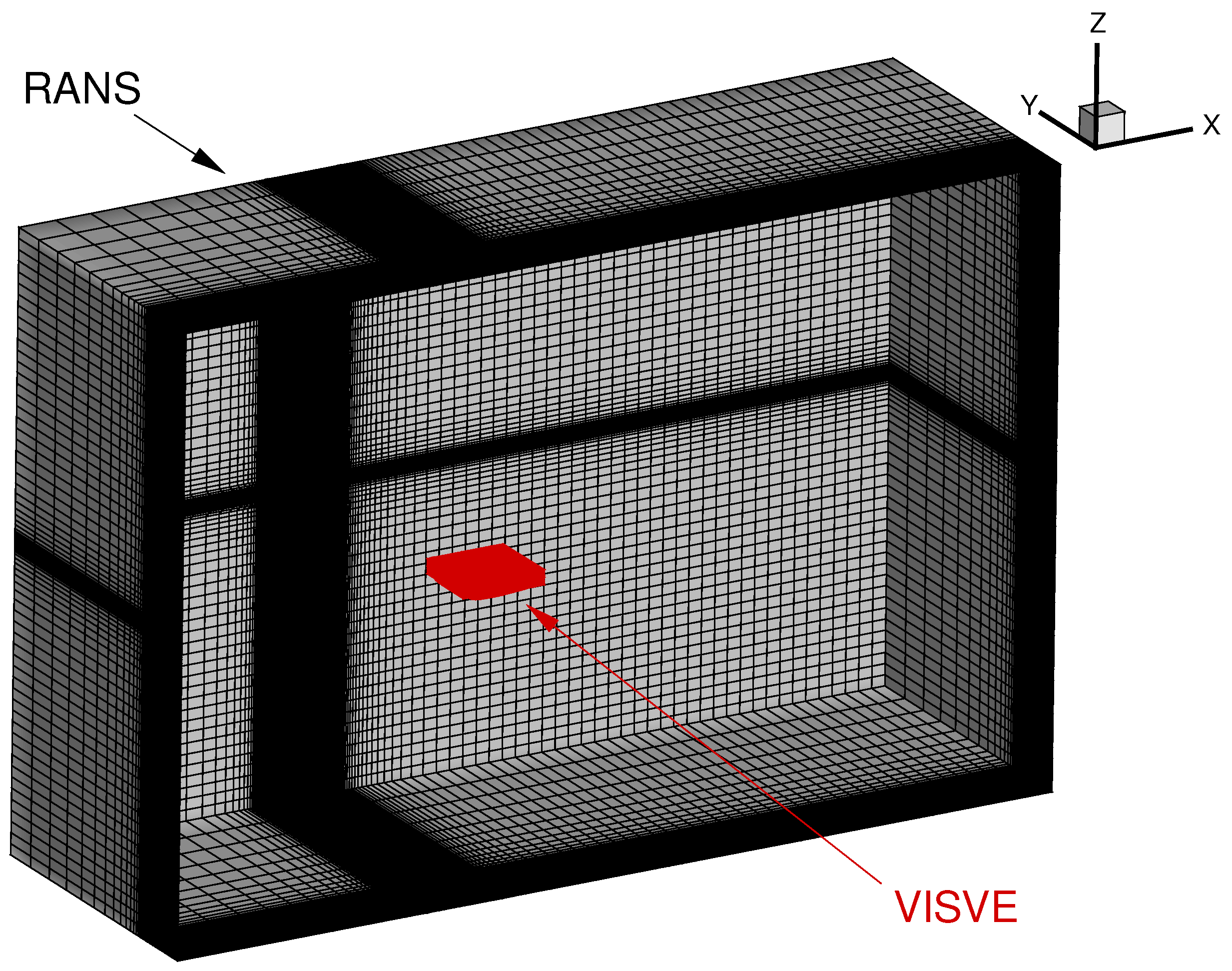
Figure 7.
Grid convergence test for velocity profiles in different chordwise directions, y/c = 0.2, AOA = , Re = .
Figure 7.
Grid convergence test for velocity profiles in different chordwise directions, y/c = 0.2, AOA = , Re = .
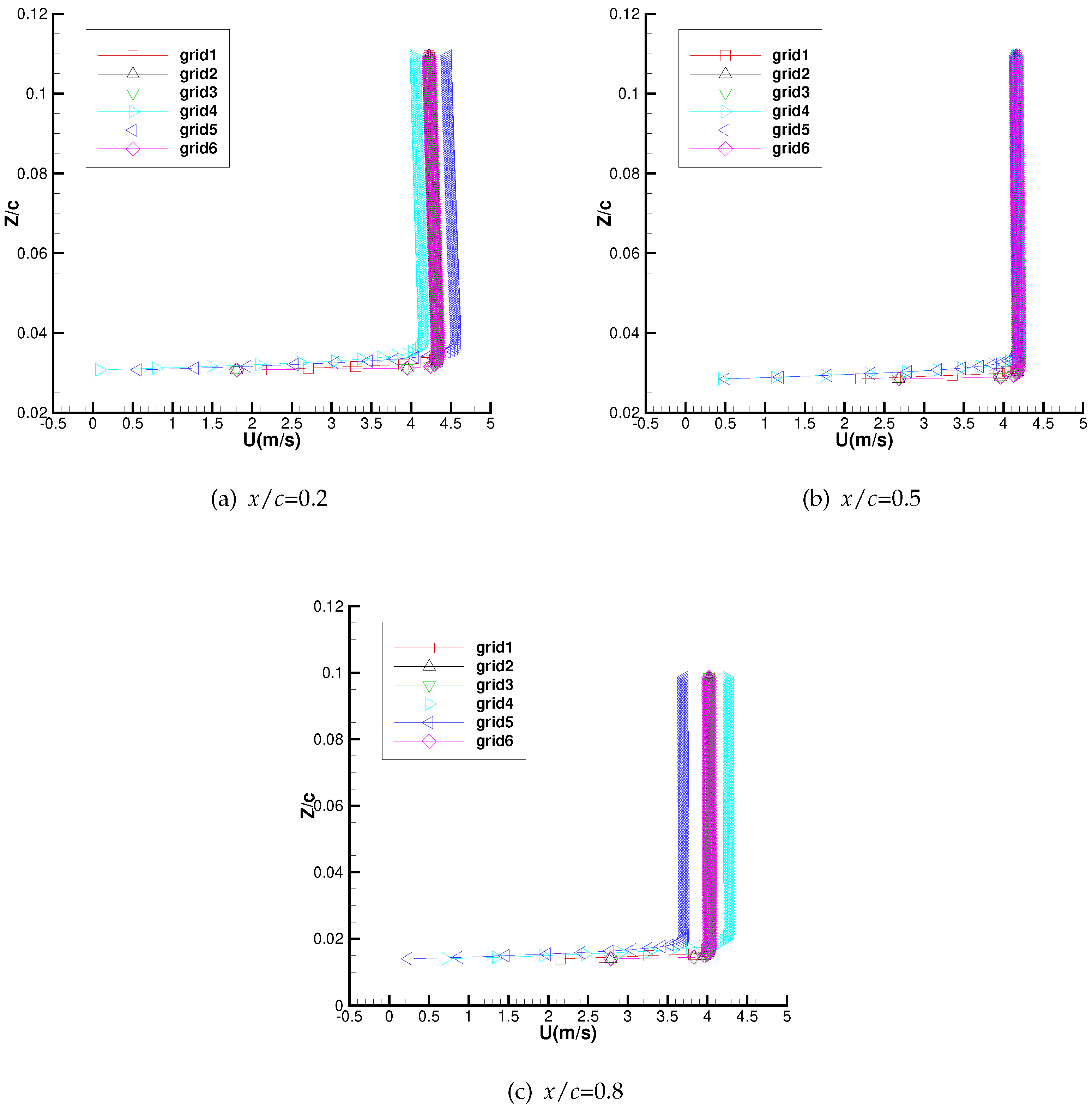
Figure 8.
Grid convergence test for velocity profiles in different spanwise directions, x/c = 0.5, AOA = , Re = .
Figure 8.
Grid convergence test for velocity profiles in different spanwise directions, x/c = 0.5, AOA = , Re = .
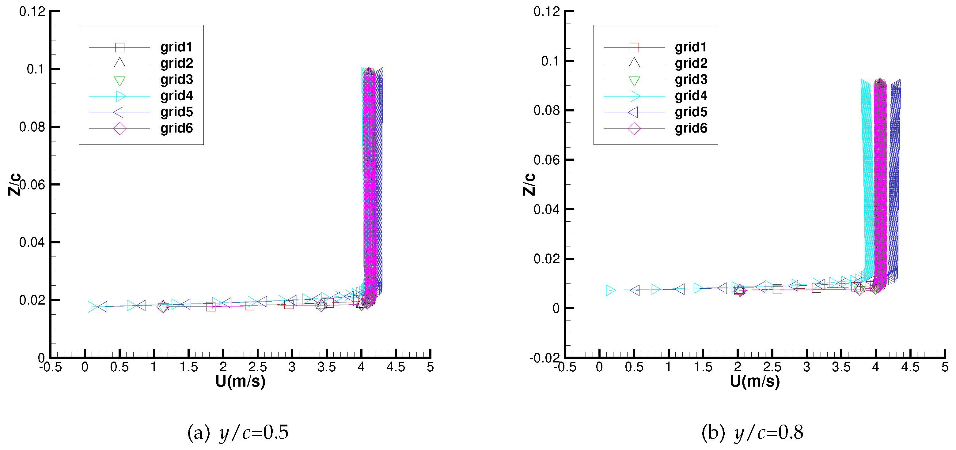
Figure 9.
Computational domain with different length of wake.
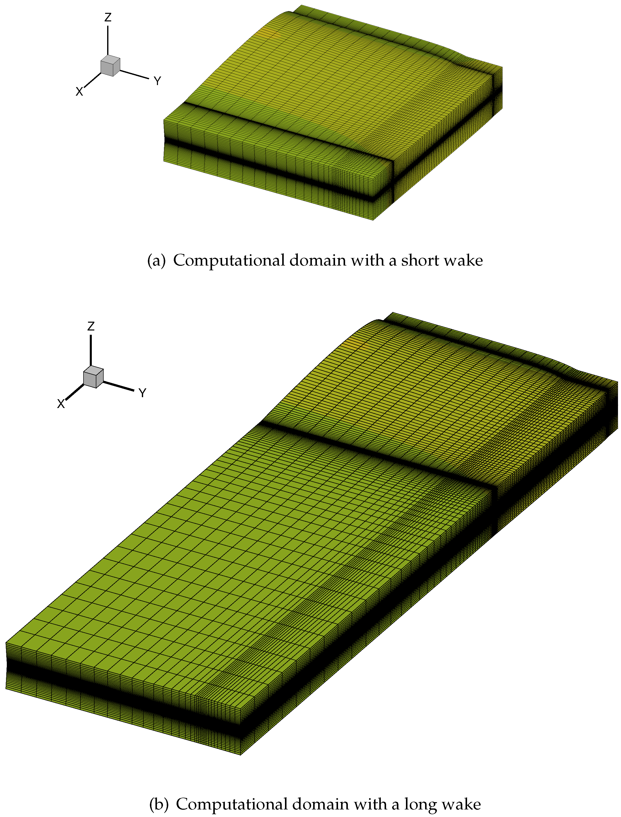
Figure 10.
Grid convergence test with respect to different length of wake, x/c = 0.2, y/c = 0.5, AOA = , Re = .
Figure 10.
Grid convergence test with respect to different length of wake, x/c = 0.2, y/c = 0.5, AOA = , Re = .
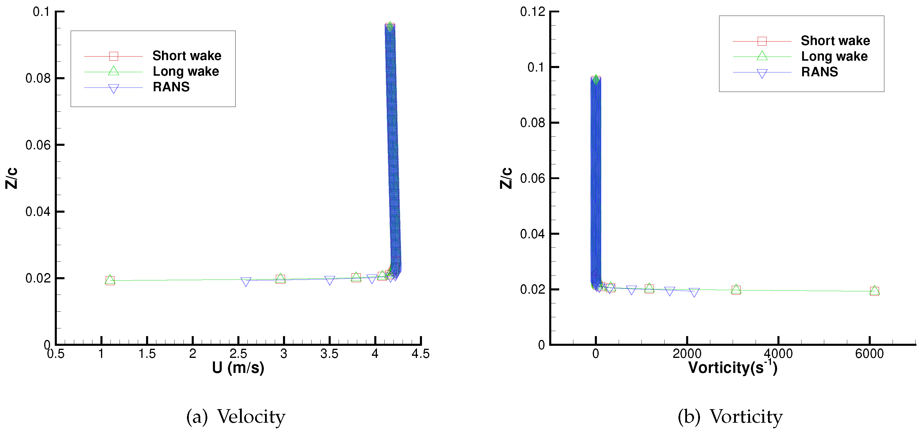
Figure 11.
Grid convergence test with respect to different length of wake, x/c = 0.5, y/c = 0.5, AOA = , Re = .
Figure 11.
Grid convergence test with respect to different length of wake, x/c = 0.5, y/c = 0.5, AOA = , Re = .
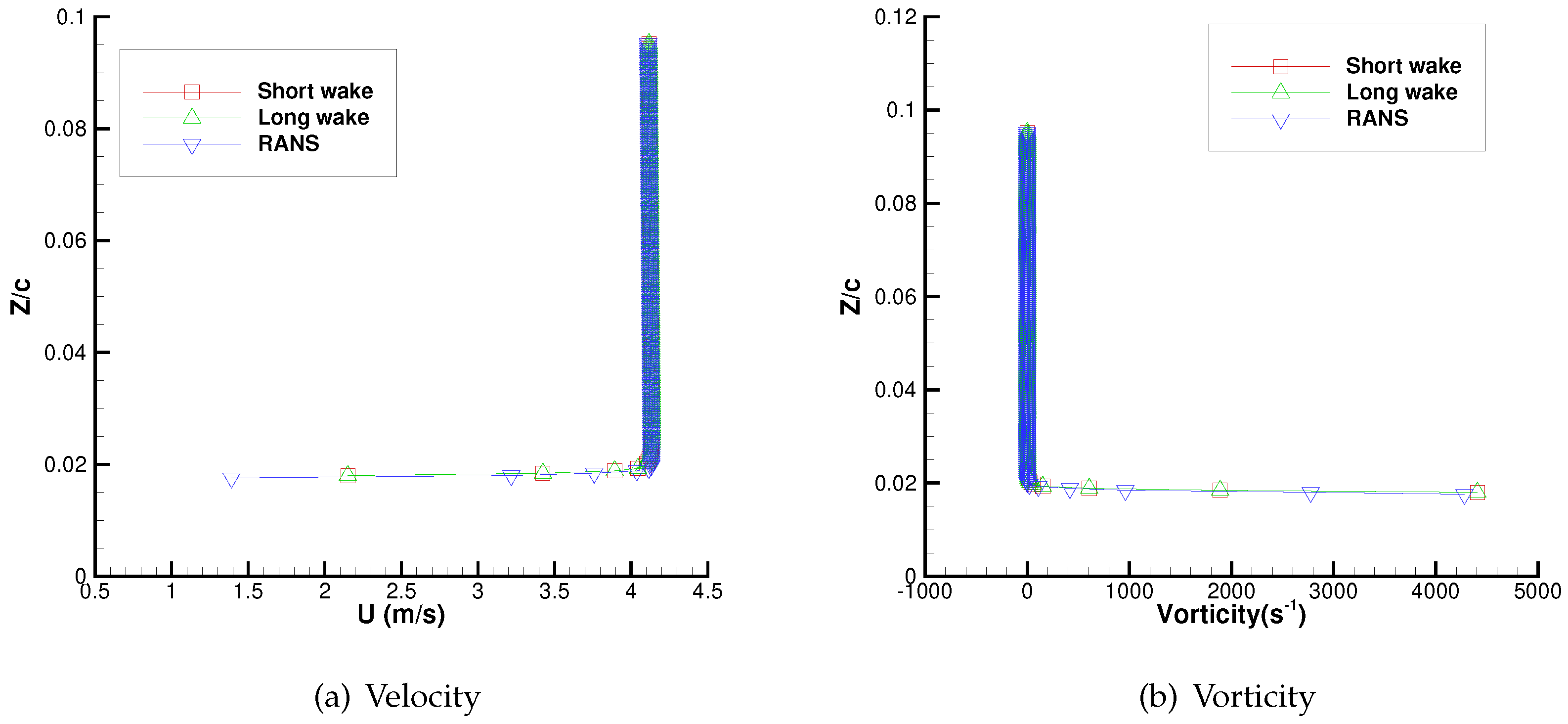
Figure 12.
Grid convergence test with respect to different length of wake, x/c = 0.8, y/c = 0.5, AOA = , Re = .
Figure 12.
Grid convergence test with respect to different length of wake, x/c = 0.8, y/c = 0.5, AOA = , Re = .
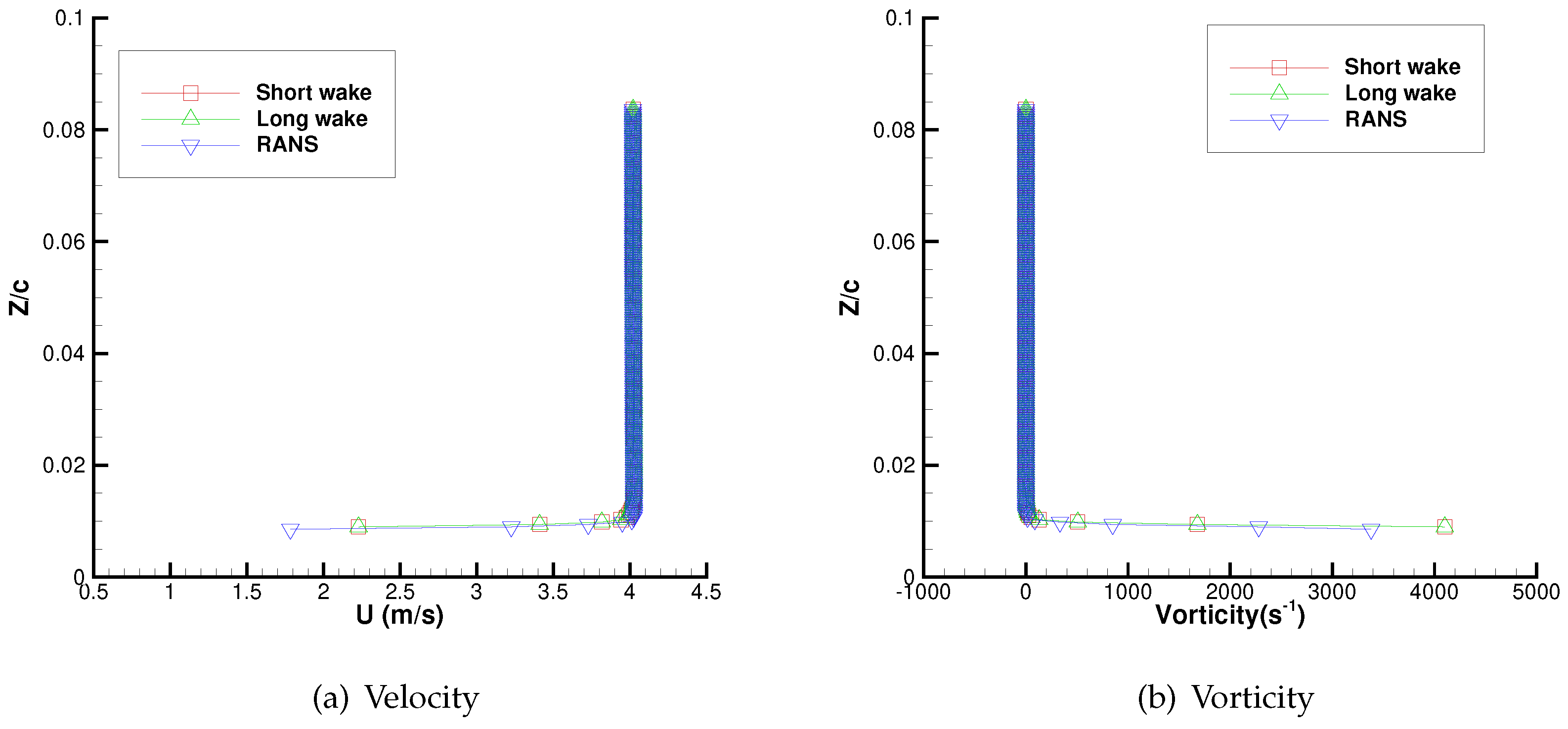
Figure 13.
Grid convergence test with respect to different length of wake, x/c = 0.5, y/c = 0.2, AOA = , Re = .
Figure 13.
Grid convergence test with respect to different length of wake, x/c = 0.5, y/c = 0.2, AOA = , Re = .
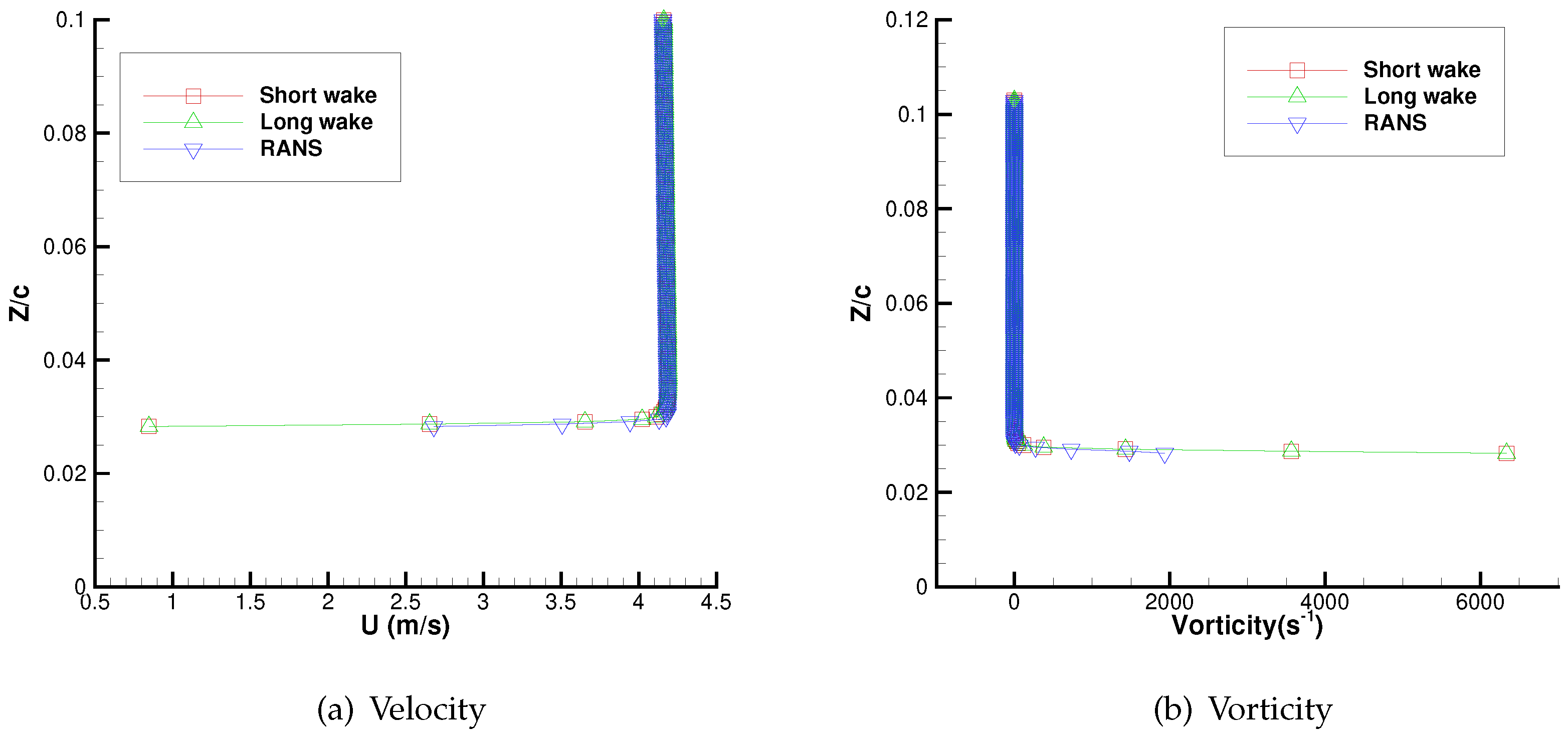
Figure 14.
Grid convergence test with respect to different length of wake, x/c = 0.5, y/c = 0.8, AOA = , Re = .
Figure 14.
Grid convergence test with respect to different length of wake, x/c = 0.5, y/c = 0.8, AOA = , Re = .
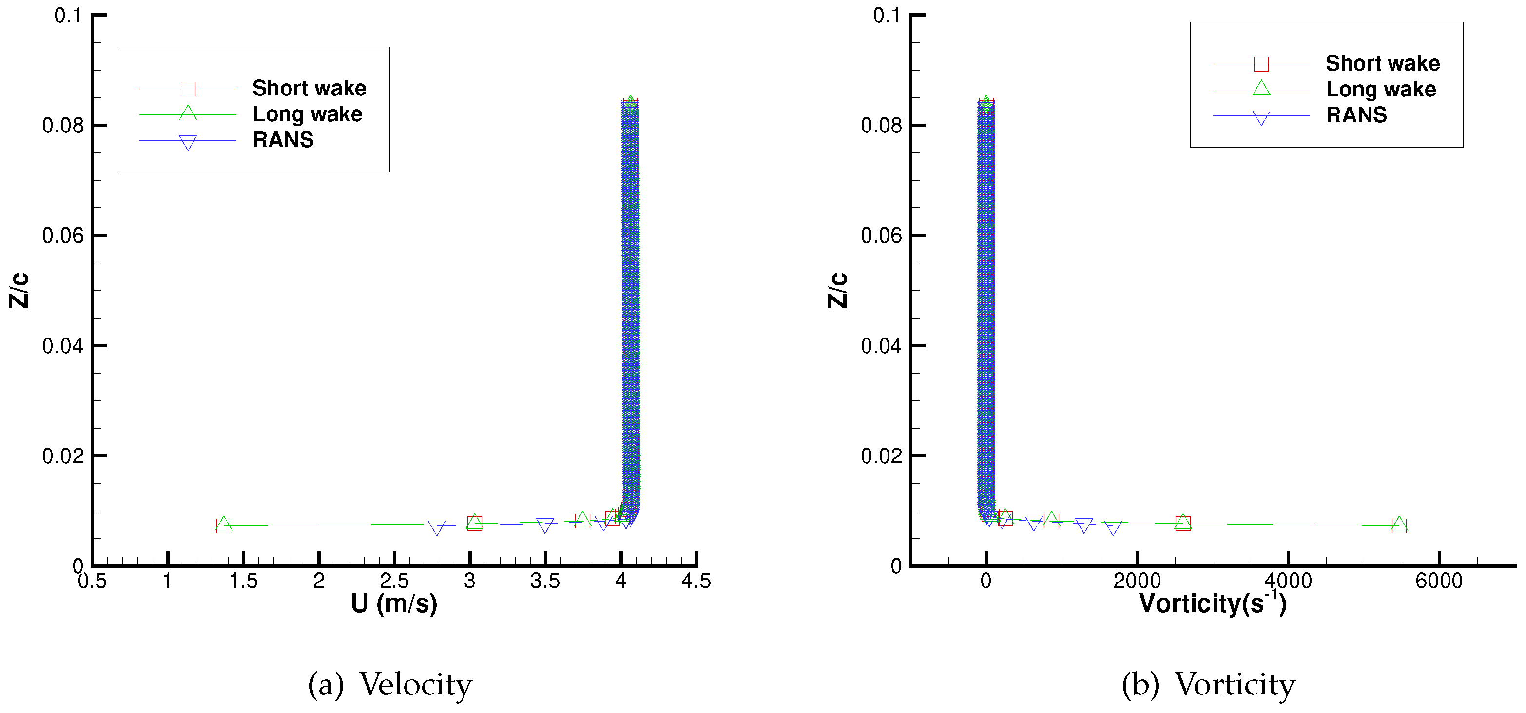
Figure 22.
Comparison of the velocity contours between 3-D Turbulent VISVE and RANS. Re= , AOA=, t = 0.01 s.
Figure 22.
Comparison of the velocity contours between 3-D Turbulent VISVE and RANS. Re= , AOA=, t = 0.01 s.
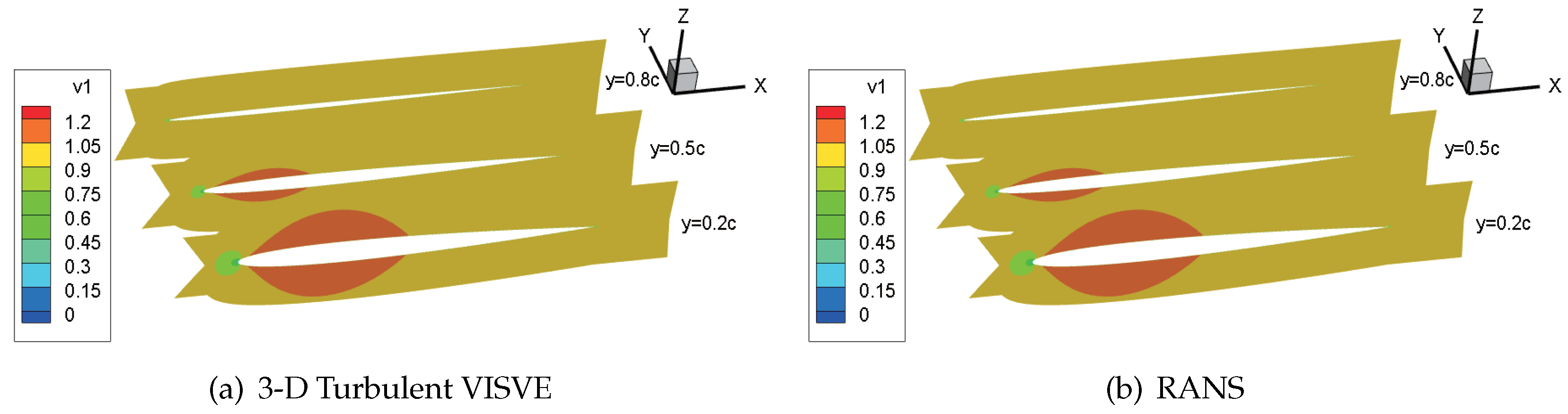
Figure 23.
Velocity profiles along x/c=0.5, y/c=0.2, 0.5, 0.8. Re=, AOA=, # of time steps = 100.
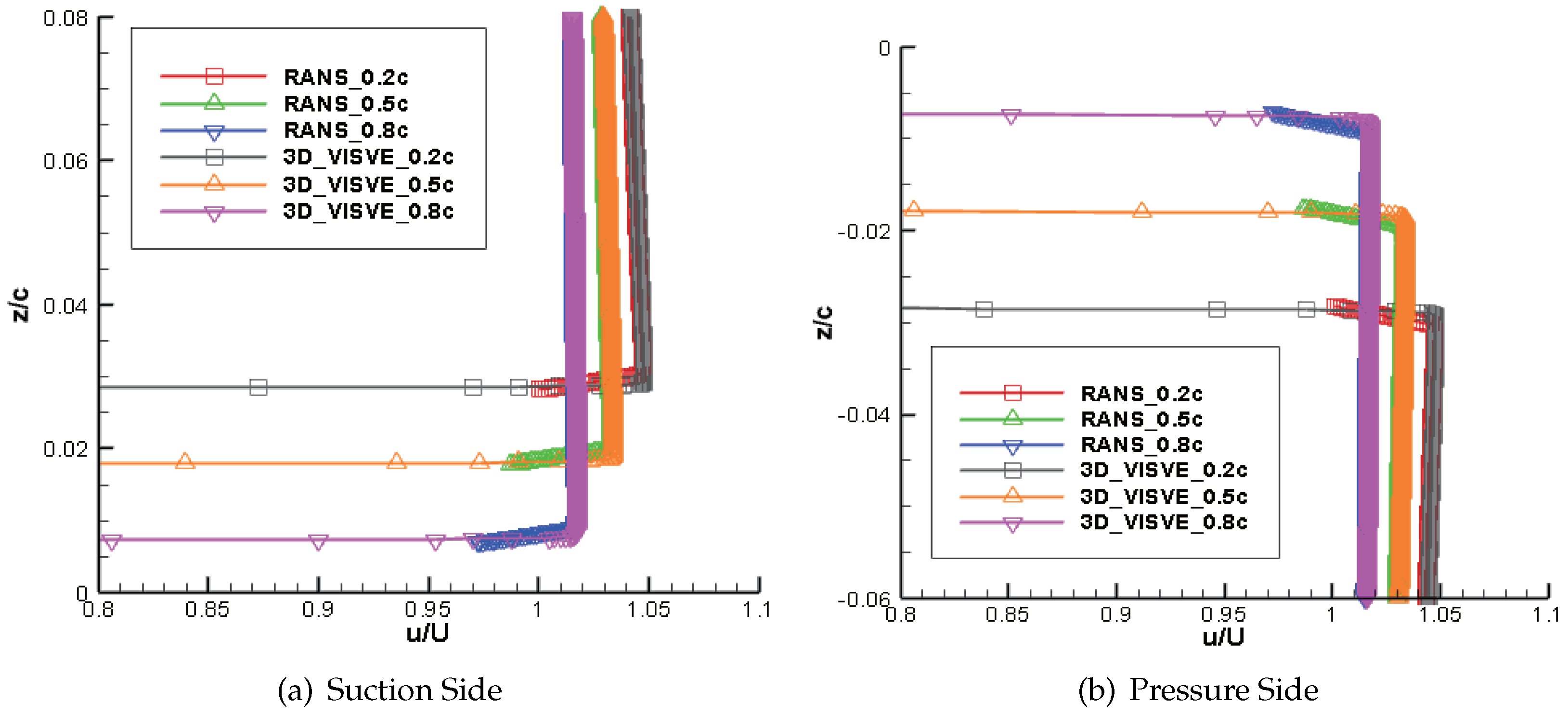
Figure 24.
Velocity profiles along x/c=0.5, y/c=0.2, 0.5, 0.8. Re=, AOA=, # of time steps = 100.
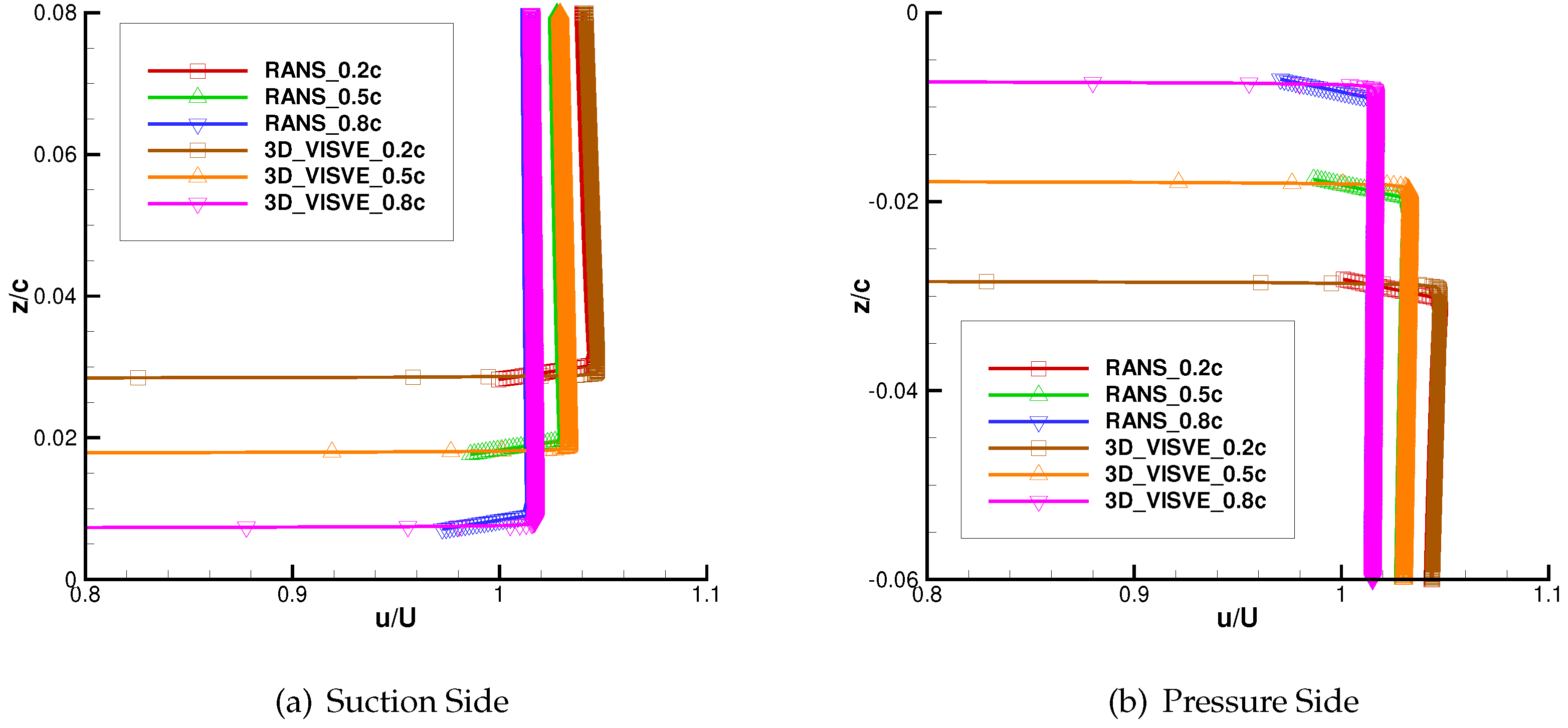
Figure 25.
Comparison of the velocity contours between 3-D Turbulent VISVE and RANS. Re= , AOA=.
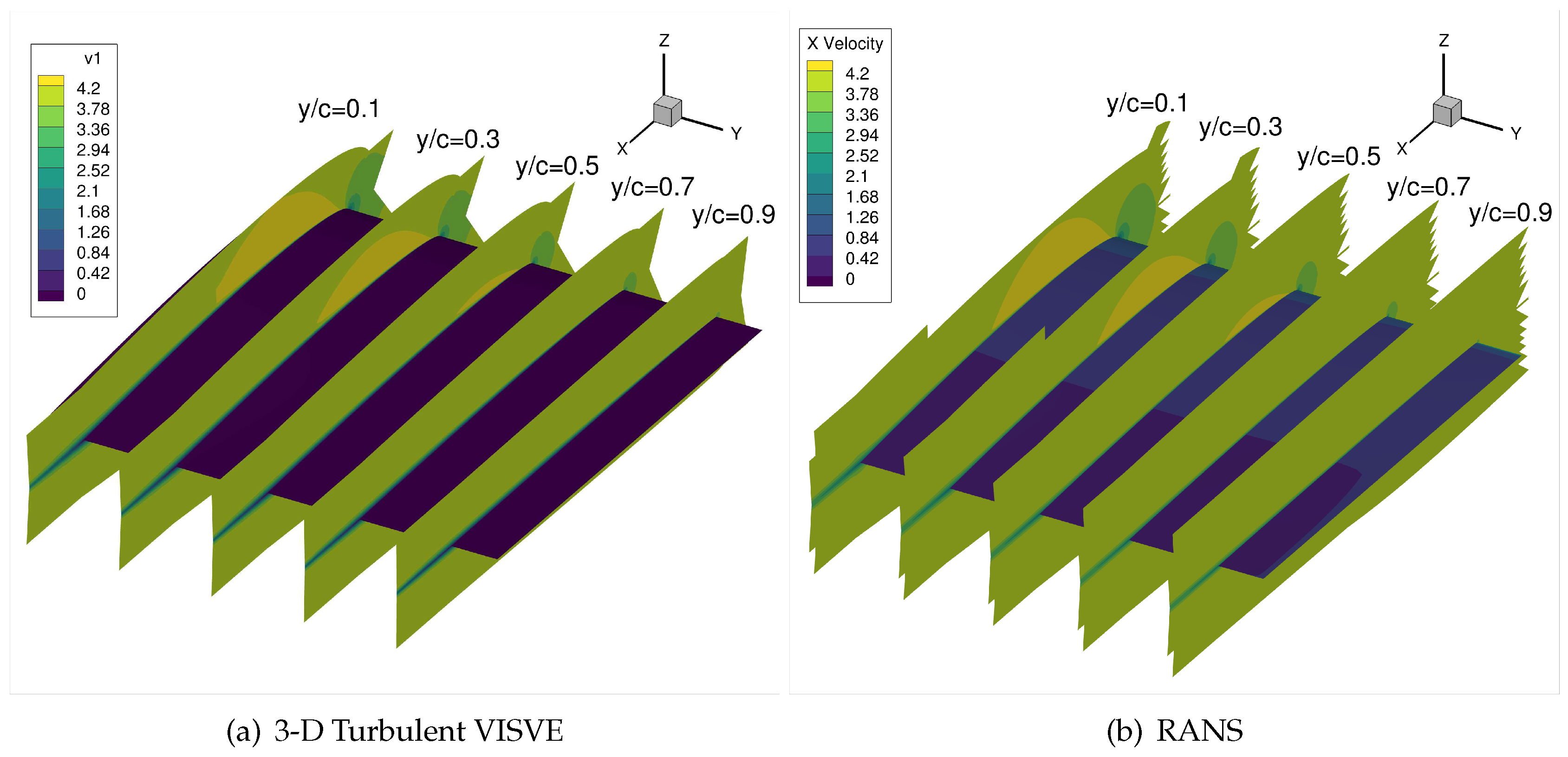
Figure 26.
Comparison of the vorticity contours between 3-D Turbulent VISVE and RANS. Re= , AOA=.
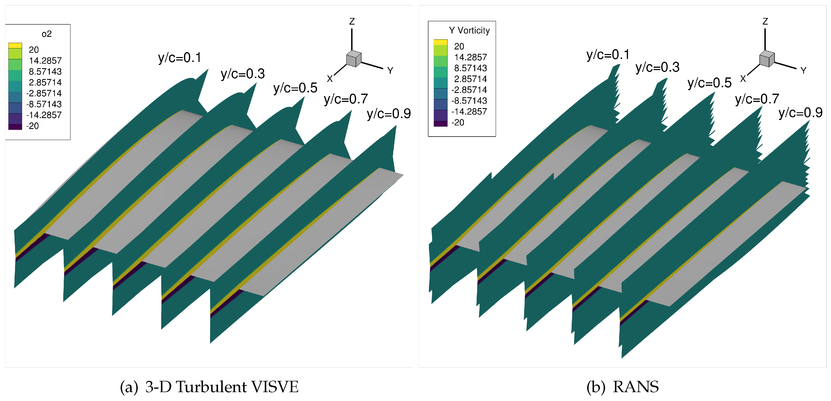
Figure 33.
Pressure distribution on the hydrofoil along different spanwise direction y/c=0.3, 0.5, 0.7, 0.9. Re=, AOA=, steady.
Figure 33.
Pressure distribution on the hydrofoil along different spanwise direction y/c=0.3, 0.5, 0.7, 0.9. Re=, AOA=, steady.
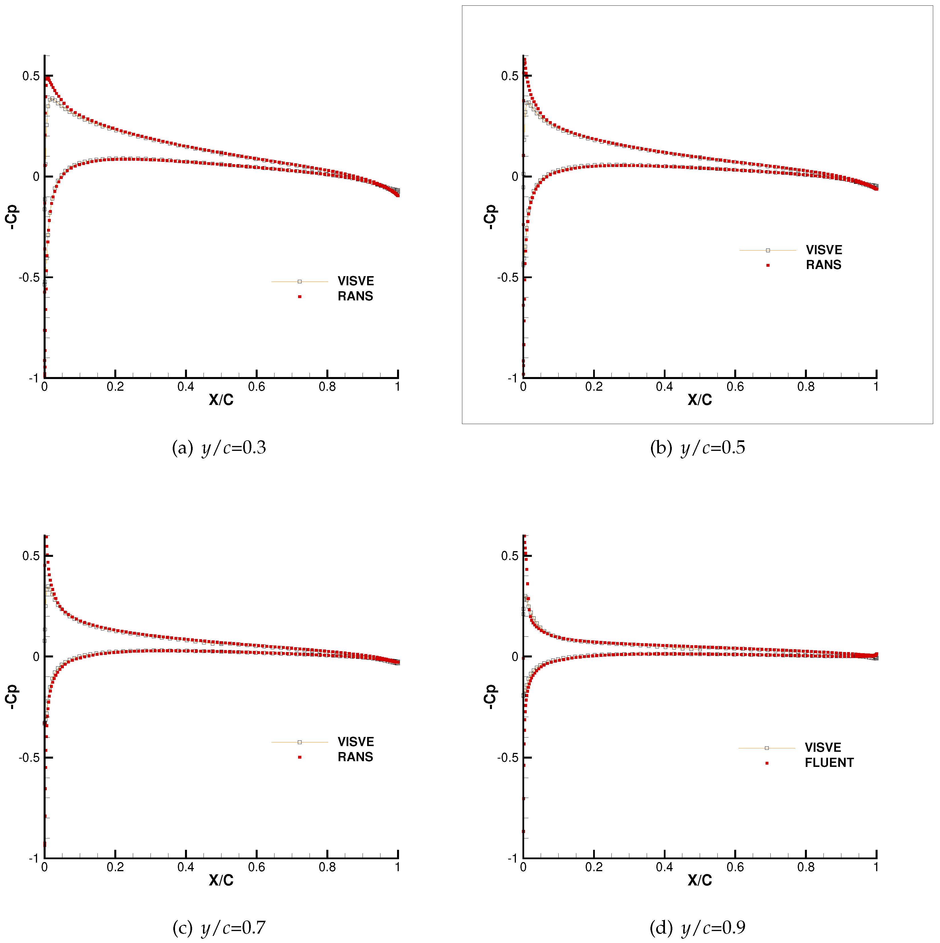

Table 1.
PARDISO Solver Parameters
| Parameter | Description |
|---|---|
| iparm(1)=1 | No default value is used. |
| iparm(2)=2 | Fill-in reordering from METIS. |
| iparm(3)=24 | Numbers of processors. |
| iparm(4)=0 | No iterative-direct algorithm is used. |
| iparm(5)=0 | No user fill-in reducing permutation. |
| iparm(8)=9 | Number of iterative refinement steps. |
| iparm(10)=13 | Perturb the pivot elements with . |
| iparm(11)=1 | Use nonsymmetric permutation and scaling. |
| iparm(13)=1 | Maximum weighted matching algorithm is switched on. |
| iparm(18)=-1 | Output: number of nonzeros in the factor LU. |
| iparm(27)=1 | Check the input matrix. |
Table 2.
Computational Settings in Fluent
| Setting | Value/Description |
|---|---|
| Solver | Pressure-Based, Segregated Flow |
| Turbulence Model | k- SST |
| Numerical Scheme | Second Order Upwind |
| Pressure-Velocity Coupling | SIMPLE |
| Time Step | 1e-4 s |
| Convergence Criteria | Residuals < 1e-6 |
| Initialization Method | Initialize from Inlet |
| Boundary Conditions | Velocity inlet; Pressure outlet; Non-slip at wall; Symmetric at midchord |
| Mesh Type | Structured |
| Grid Refinement | Manual |
Table 3.
Comparison of the mesh and the computational time between VISVE and RANS for the rectangular wing.
Table 3.
Comparison of the mesh and the computational time between VISVE and RANS for the rectangular wing.
| VISVE | RANS | |
|---|---|---|
| Mesh | 199,680 | 2,342,640 |
| Computational time/iter | 5.7 s | 22 s |
| No. of CPUs | 40 | 40 |
Table 4.
Grids employed for the convergence test in the wing case.
| Grid | x | y | z | Total grids |
|---|---|---|---|---|
| 1 | 64 | 20 | 30 | 199,680 |
| 2 | 64 | 20 | 46 | 306,176 |
| 3 | 84 | 20 | 46 | 365,056 |
| 4 | 44 | 20 | 46 | 247,296 |
| 5 | 64 | 15 | 46 | 258,336 |
| 6 | 64 | 30 | 46 | 401,856 |
Table 5.
Time steps employed for the convergence test in the wing case.
| Case | Time step |
|---|---|
| 1 | 0.00005 s |
| 2 | 0.0001 s |
| 3 | 0.0002 s |
Disclaimer/Publisher’s Note: The statements, opinions and data contained in all publications are solely those of the individual author(s) and contributor(s) and not of MDPI and/or the editor(s). MDPI and/or the editor(s) disclaim responsibility for any injury to people or property resulting from any ideas, methods, instructions or products referred to in the content. |
© 2023 by the authors. Licensee MDPI, Basel, Switzerland. This article is an open access article distributed under the terms and conditions of the Creative Commons Attribution (CC BY) license (http://creativecommons.org/licenses/by/4.0/).
Copyright: This open access article is published under a Creative Commons CC BY 4.0 license, which permit the free download, distribution, and reuse, provided that the author and preprint are cited in any reuse.