

Submitted:
07 December 2023
Posted:
07 December 2023
You are already at the latest version
Abstract
This article investigates hydraulic percolation in saturated porous media, focusing on containment systems using sheet pile walls and gravity concrete dams. The Laplace equation, which governs hydraulic flow in porous media, is solved using the Finite Element Method through the ANSYS software. The modeling of the porous media employs a planar quadratic element called Plane 55, originally used for thermal problems, composed of four nodes and one hydraulic degree of freedom per node. The numerical results of the water pressure acting on the hydraulic structure, flow rate, and hydraulic gradient at the outlet of the porous media are compared with results obtained in the technical-scientific literature using flow nets. Two different methodologies are used to obtain the rate of seepage: by using the average hydraulic velocity or by calculating the integral of the hydraulic gradient perpendicular to the flow area. Both methodologies are compared and validated in the numerical simulations. This work also demonstrates the importance of mesh refinement for obtaining the flow rate in the studied hydraulic systems.
Keywords:
Soil hydraulics
; FEM
; Laplace equation
; steady-state regime.
1. Introduction
Water percolation failure in rocky and earthen masses can lead to severe geotechnical disasters, such as the collapse of water and tailings dams, the breaching of dykes and road tunnels, and the formation of craters on roads [1,2,3]. The risk of percolation failure in porous mediums also exists in urban projects, for instance, in underground parking lots and tunnels for metro implementation, essentially in any structure involving deep excavations and lowering of the groundwater table [4,5]. The mechanisms of percolation-induced failures in porous mediums are not yet fully understood, owing to the wide variety and complexity of interactions between fluids and soils [6]. A deeper understanding of percolation failure mechanisms is believed not only to enable the prediction of potential disasters but also to contribute to the effective control of construction processes.
Among the various geotechnical solutions available for controlling hydraulic flow in porous mediums, gravity concrete dams, and sheet pile walls are widely employed. Gravity concrete dams are massive structures made of reinforced or cyclopean concrete designed to withstand the pressure generated by the hydrostatic force of water through their own weight. They are typically constructed in locations with access to suitable construction materials, such as rocks or competent soils. On the other hand, sheet pile walls consist of prefabricated elements, usually made of steel, driven vertically into the ground to form a continuous wall capable of restraining soil movement and water percolation. They are used in projects requiring temporary or permanent containment, in deep excavations, in tunnels, and coastal areas, allowing for faster construction compared to gravity concrete dams.
Understanding the hydraulic behavior of the porous media is essential to assess the efficiency of the hydraulic containment system and ensure its stability and safety, as well as the protection of the surrounding environment.
The study of hydraulic behavior involves analyzing the water pressure on the faces of the containment, determining hydraulic gradients in the porous medium, and quantifying the amount of water percolating (hydraulic flow) downstream of the containment system, among other factors.
In this context, the Finite Element Method (FEM) has proven to be a widely used tool in the technical-scientific field for the numerical analysis of hydraulic flow in porous media within various hydraulic structures. This is due to the complexity of materials involved in such projects and the absence of analytical formulations for more complex practical problems [7,8]. With the FEM, adjustments and modifications can be made to the hydraulic and geotechnical properties of the porous medium, such as specific weight, hydraulic permeability coefficient, and water level position, among other aspects. Moreover, the FEM allows alterations in the boundary conditions of the porous medium and the materials used in the construction of the groundwater barrier.
The numerical study, through FEM, of hydraulic percolation in porous media using different hydraulic containment systems is addressed in various studies, such as those referenced in [6,9,10,11]. These works have demonstrated that, despite being a field of study for many centuries, the technical-scientific interest in this subject continues to evolve and renew itself over the years.
This article presents a study of hydraulic flow in a porous, isotropic, and saturated medium under steady-state conditions, employing either sheet pile walls or gravity concrete dams. These hydraulic systems are modeled using FEM in the ANSYS APDL software, and the numerical results obtained are compared with those provided in technical-scientific literature, using graphical methods involving flow nets.
The hydrostatic water pressure acting on the groundwater barrier, flow rate and exit gradient at the porous medium are determined.
Few technical-scientific studies address this comparative aspect between graphical methodologies, using flow net, and numerical approaches employing the Finite Element Method (FEM). Flow nets are predominantly found in didactic materials. Moreover, a limited number of studies utilize the proposed software in this work due to its lack of exclusive dedication to hydraulic flow problems.
2. Soil Hydraulics
There are several ways to obtain solutions for two-dimensional percolation problems, ranging from exact or analytical solutions for specific scenarios to graphical solutions such as flow nets and approximate numerical solutions like Finite Difference Methods (FDM) and Finite Element Methods (FEM). This study will focus on graphical methods and FEM.
Regardless of the method used, the aim is typically to approximate the particular solution of a hydraulic flow problem in a porous medium, which in two-dimensional form can be described by the differential equation:
where is the total hydraulic head, , and are principal permeability coefficients, and represent the degree of saturation and the void ratio of the porous medium, respectively, and is the variable associated with time.
Assuming the hypotheses that the porous medium is homogeneous, isotropic, saturated, and does not undergo compression or expansion over time, from the first hypothesis: and ; from the second hypothesis: , finally, from the last hypothesis: and .
Adopting these three hypotheses in Equation (1) results in the following simplified differential equation:
which is known as the Laplace’s differential equation, governing steady 2D flow, respecting the previously mentioned assumptions.
The velocity of hydraulic flow in a two-dimensional medium under laminar conditions can be calculated using Darcy’s law:
The graphical solution of Equation (2), according to [12], was developed in 1930 by Forchheiner and became widely used in the design of dams and dikes from around 1940 onwards. This solution consists of two families of curves, and , known respectively as the velocity potential function and the stream function (or flow function). In porous and isotropic mediums, these curves intersect at right angles (orthogonal trajectories). Curves with constant values of are termed equipotential lines, while those with constant values of are called streamlines. The set composed of equipotential lines and streamlines constitutes the flow net.
In a flow net, the regions enclosed between two pairs of crossing streamlines and equipotential lines are referred to as elements. The total number of elements in a flow net () is given by the product , where represents the number of flow channels () while refers to the number of equipotential drops (). The ratio is defined as the shape factor of the flow net.
In a flow net, the rate of seepage (flow rate or discharge) can be calculated according to the expression:
where is the coefficient of hydraulic permeability (or conductivity) of the porous medium, and is the total head loss dissipated between the extreme equipotential curves of the flow net. is given by the difference between the downstream hydraulic head () and the upstream head () of the system.
The flow rate is measured per unit length of the flow net, in the International System of Units (SI), expressed as m3/s/m. Meanwhile, the coefficient of hydraulic permeability (permeability) of the porous medium (measured in m/s in SI) is obtained experimentally using devices called permeameters, which can be a constant or variable head.
Besides discharge, another important hydraulic parameter in the study of hydraulic flow in porous media is the hydraulic gradient, defined in a two-dimensional flow by the expression:
In a flow net, hydraulic gradients can be obtained in any of its constituent elements through the expression:
where is the length of the element in the direction of the flow, and in this case is the head loss in the element.
Calculating the hydraulic gradient at the outlet (downstream) region of the flow net can help prevent conditions such as percolation liquefaction (quicksand phenomenon) and the occurrence of internal erosion, which involves the transport of particles within the porous medium.
The critical hydraulic gradient, , which leads to the liquefaction of the porous medium, is given by the expression [13]:
where is the submerged unit weight of the porous medium (), with being the unit weight of water.
Since in most soils, the submerged unit weight is equal to that of water, that is, , the is approximately unity, representing a situation that must be avoided in engineering projects [13].
The recommended safety factor in percolation problems is around 3 to prevent the liquefaction phenomenon. Therefore, the exit gradient obtained from Equation (7) should be less than 0.3 [13]. Additionally, as noted by the same author, high gradients can cause internal erosion, also called piping, and should thus be avoided.
Another important parameter in the study of percolation in porous media is the water pressure head () that can occur at the hydraulic structure. This component can be obtained through the expression:
where is the total hydraulic head at a chosen point in the porous medium, is its altimetric head, and is the piezometric head at the analyzed point in the system. In this expression, the altimetric head is equal to the elevation of the soil element concerning to a reference, while the component related to the piezometric head can be obtained through the expression:
where is the pore pressure at the analyzed point. The pore pressure distributed along the contact interface between the massif and the hydraulic structure constitutes the water pressure ().
In addition to the use of flow nets, as previously mentioned, the study of hydraulic flow in a porous medium can be conducted using the Finite Element Method (FEM). After applying boundary conditions involving the imposition of hydraulic gradients and hydraulic loads at the model’s borders, the numerical computation of flow rate () in FEM typically involves obtaining the value of the fluid percolation velocity component () perpendicular to a conveniently chosen cross-section () of the porous medium.
The rate of flow obtained through a section , located in the y-direction of a homogeneous and isotropic porous medium, can be determined by the analytical expression (adapted from [12]):
The integral provided in Equation (10) can be solved by summing the trapezoids constructed with successive gradients obtained between the integration limits and , using the trapezoidal rule for numerical quadrature [12]. These limits correspond to the vertical boundaries of the unit-length area in the z-direction.
The final form of Equation (10) depends on the position within the porous medium of the analyzed section. In the case of a horizontal section, the definite integral defined by Equation (10) can be rewritten as (adapted from [12]):
In the FEM, alternatively, the analytical Equations (10) and (11) are solved using the average hydraulic velocity obtained between the limits and of Equation (10), or and of Equation (11), leading to more simplified expressions [14]:
where and are the average horizontal and vertical velocities perpendicular to the areas and , respectively.
3. Methodology
Two distinct hydraulic structures, a sheet pile wall, and a gravity concrete dam, are modeled using the Finite Element Method (FEM) in the ANSYS APDL software to study seepage through a saturated, homogeneous, and isotropic porous medium.
The hydraulic flow will be studied to determine the flow rate of the system (), the exit hydraulic gradient (), and the hydraulic uplift pressure () acting on the faces of the hydraulic structure.
For the two-dimensional modeling of these systems, quadratic planar finite elements will be used, composed of four nodes and one hydraulic degree of freedom per node, called Plane 55 in ANSYS.
The numerical results obtained via FEM will be compared and confronted with data using the graphical method based on the flow net available in the technical-scientific literature.
Specifically the hydraulic flow rate, by graphical method, using flow net and Equation (4). On the other hand, in the FEM, the flow rate is obtained through the expressions provided by Equations (10-12).
Equation (12) allows the rate of seepage calculation through the average velocity perpendicular to a specific surface, while the analytical expressions defined by Equations (10) and (11) are used to calculate the flow rate through the integrals and , respectively.
As Equations 10, 11, and 12 are solved by exporting the data of hydraulic gradients ( and ), obtained in the ANSYS software after solving the Equation (2), via Matlab. Numerical integration is performed using the trapezoidal rule employing the «trapz» command, and the average velocities are obtained using the «mean» command in Matlab.
4. Numerical Simulations
4.1. Sheet Pile Walls
Ongoing studies have explored seepage flow thought a porous medium containing a cantilever sheet pile wall, as depicted in Figure 1, using flow nets [13,15,16].
In Figure 1, nine equipotential lines (ψ) and five streamlines () of the porous medium are illustrated, resulting in eight equipotential drops () and four flow channels ().
The works in the technical-scientific literature differ in the hydraulic head adopted upstream () and downstream () of the hydraulic structure, consequently leading to variations in the hydraulic head (). Additionally, they differ in permeability () and width () adopted for the porous medium, in the thickness (), and in the embedment depth (segment f of the sheet pile wall inserted in the porous medium). This also includes the depth between the base of the sheet pile wall and the impermeable porous medium (), as schematically illustrated in Figure 1.
Table 1 presents the hydraulic and geotechnical parameters utilized in the studies employing flow nets conducted by [13,15,16]. These same parameters are employed in the numerical models based on the FEM proposed in this work, denoted as MEF-O, MEF-D, and MEF-CS, according to the initials of each of the previously mentioned authors.
Some geometric parameters provided in Table 1 were estimated since they were not directly available in the mentioned studies.
According to Table 1 and in accordance with [13], it is observed that the porous medium implemented in the MEF-O model features very low permeability, ranging from , considered impermeable. Conversely, in the MEF-D model, the porous medium exhibits low permeability, ranging from , while in the MEF-CS model, it presents high permeability, ranging from , thus considered permeable porous mediums.
Figure 2 illustrates the discretization of the finite element mesh of the porous medium in the MEF-D model. In this mesh, quadratic planar elements with a constant dimension of 0.25 m were used, resulting in a total of 9214 hydraulic degrees of freedom.
Figure 3 illustrates the equipotential surfaces obtained using the MEF-D after solving Equation (2).
In observing Figure 2 and Figure 3, it is possible to notice that the hydraulic head of equipotential surface MM’, located upstream in the porous medium, is equal to 16.6 m (a value obtained from , as provided in Table 1), taking the x-y system illustrated in Figure 2 as reference. On the other hand, at the outlet JJ’ of the porous medium, the hydraulic head assumes the value of 13.2 m (a value obtained from provided in Table 1).
The flow rates obtained through flow nets as per [13,15,16] are respectively equal to 6.74 x 10⁻⁵, 1.13 x 10⁻⁶, and 1.25 x 10⁻³ m3/s/m, conform Table 2. In addition to these discharges obtained graphically, the numerical modeling of porous media via FEM resulted in flow rates indicated in Table 2, columns four and five.
The flow rates presented in Table 2 are calculated considering two distinct areas of 1 m width along the z-direction, perpendicular to the x-y plane illustrated in Figure 2. The area between the base of the sheet piles and the impermeable medium, OO’ depicted in Figure 2, is equal to P’Q. On the other hand, the downstream area of the porous medium is equal to JJ’.
The rate of seepage is obtained for the two sections P’Q and JJ’ using the average percolation velocity (VM), as provided by Equation (12). Additionally, it is obtained through analytical calculation of the integral of the hydraulic gradient (GH), as described by Equations (10) and (11).
Table 2 compares the flow rates numerically obtained by FEM using these two methodologies (VM and GH) with the analytical value obtained via flow net (RF), provided in the works of [13,15,16]. The percentage differences between the flow rate obtained by the graphical method and by FEM are provided in the sixth and seventh columns of Table 2.
Upon analyzing Table 2, it is noticeable that methodologies employing VM and GH for calculating hydraulic flow rate present values close to each other, regardless of the P’Q and JJ’ sections analyzed. Additionally, it is observed that, except for the P’Q section of the model proposed by [16], the hydraulic flow rate obtained by FEM (using VM and GH) is lower than that obtained by the graphical method (RF). Regarding the percentage difference of the flow rates calculated using the numerical and graphical methods, it is noted that the percentage difference is high, ranging between 4.72% to 22.72%.
Importantly, before presenting the hydraulic flow rates obtained via VM or GH for the P’Q and JJ’ sections analyzed in Table 2, a mesh convergence analysis associated with the hydraulic flow was performed for the three FEM models, MEF-D, MEF-O, and MEF-CS implemented in this study. This analysis involved studying the curves relating to the number of degrees of freedom (ndf) versus Q, illustrated in Figure 4, Figure 5, and Figure 6.
For the three implemented numerical models, convergence of flow rate values was observed when using a mesh with approximately 1000 hydraulic number of degrees of freedom (ndf). However, during the conducted numerical analyses, a high concentration of hydraulic gradients was observed in the vicinity of the base of the sheet pile wall, leading to non-convergence of data when using a coarser mesh in this area. To address this issue, a finer discretization of elements near the base of the sheet pile wall was chosen, resulting in the flow rate convergence. It is important to highlight that, in these situations, a less refined mesh was also chosen for the remaining regions of the porous medium, aiming to reduce the computational processing cost of the numerical models.
Figure 7 illustrates the distribution of the hydraulic gradient throughout the porous medium. From Figure 7(a), it can be observed that by using a mesh with elements of constant dimensions of 0.25 m (totaling 4607 ndf), the maximum resulting hydraulic gradient is 0.964 and occurs at the base of the sheet pile wall.
Figure 7(b) illustrates the importance of mesh convergence analysis, as refining only the region around the base of the wall (using elements four times smaller) while maintaining the other elements with constant dimensions of 0.25 m, the maximum resulting hydraulic gradient increases to 2.402 (with a mesh totaling 24,794 ndf), which is 149.17% higher than the previously obtained value. This discrepancy can lead to erroneous values of hydraulic flow rates, which depend on the gradient.
Table 3 presents, in columns two and three, the values of the altimetric hydraulic head () and total head () obtained by [13] through the flow net, considering different points located in the containment. The fourth column of this table provides the values obtained in this work using the FEM, with a mesh discretized with elements of constant dimensions of 0.10 m, totaling 16,546 hydraulic degrees of freedom.
The points B, E, and H provided in Table 3 and illustrated in Figure 1 are in the same location as the points M’, P’, and J illustrated in Figure 2.
The third column of Table 3 provides the total hydraulic heads obtained by [13] through the flow net, while the fourth column presents the values obtained by FEM using the MEF-O model. The points between A, B, C, and D are located along the left face of the wall, whereas sections F, G, H, and I are on the right face. Point E is situated at the base of the sheet pile wall.
Observing the data provided in Table 3, it can be noticed that the percentage error between the values obtained graphically and numerically by FEM is small, ranging between 0 to 4.77%. This error is lower at points located on the upstream face of the wall, ranging between 0 to 2.01%.
Figure 8 and Figure 9 illustrate, respectively, the upstream and downstream water pressures () acting along the sheet pile wall relative to the adopted reference level. Figure 8 illustrates the uplifts acting along the upstream face of the wall (points A, B, C, D, and E), while Figure 9 illustrates the points located along the downstream face of the wall (points E, F, G, H, and I).
The uplift pressure () is calculated using the total head () and the altimetric head (), provided in Table 3, along with the specific weight of water () as indicated by Equations (8) and (9). In the simulations presented in this work, the value of was assumed to be 10 kN/m³.
Along the upstream side of the wall, as illustrated in Figure 8, a good agreement can be observed between the water pressure () obtained by [13] when compared with the numerical values obtained by FEM in this study. However, along the downstream face of the wall, there is a small discrepancy in the values of , which tends to decrease near point H. At this point, is equal to 15 kPa. In general, upon analyzing Figure 8 and Figure 9, it is evident that the numerical simulations provide uplift pressure values that are lower than those obtained graphically by [13].
4.2. Concrete gravity dam
The present numerical simulation is based on the seepage flow through a concrete gravity dam resting on the porous medium proposed by [13], employing flow nets, as illustrated in Figure 10.
The gravity concrete dam, as illustrated in Figure 10, is subjected to an upstream hydraulic head () of 28.20 m and a downstream hydraulic head () of 20.40 m.
The flow net, illustrated in Figure 10, exhibits four flow channels () and fourteen equipotential drops (), resulting in a form factor () of 0.31. The total head loss of the system is 7.80 m (), with the drop in head between each of the thirteen adjacent equipotentials () being 0.60 m.
The permeability of the porous medium is equal to 5 x 10⁻⁹ m/s, as indicated by [13]. This represents a very low permeability, ranging between , corresponding to a typical hydraulic permeability of clay soils or rocks.
Figure 11 illustrates the numerical model of the porous medium using finite elements with a constant dimension of 0.50 m. This mesh was adopted to a better visualization of the model. However, in the numerical simulations presented below, the discretization of the numerical model of the porous medium was performed using elements of dimensions equal to 0.15 m each, resulting in a mesh with a total of 43,055 degrees of freedom.
As seen in Figure 10 and Figure 11, the concrete dam features a sheet pile wall located upstream (M’P’PA) and another downstream (FSS’J), aimed at reducing seepage through dam. The thickness of the sheet pile walls in the curtains were assumed to be constant at 0.25 m. The M’P’PA and FSS’J walls have lengths of 3.4 m and 5.65 m, respectively.
Considering the reference plane x-y, as illustrated in Figure 11, coinciding with the OO’ boundary, the boundaries MM’ and JJ’ are equipotential lines, as they possess a constant hydraulic head equal to and , respectively.
Assuming that the flow is confined to the porous medium, the remaining boundaries are impermeable. This means that the component of the velocity vector perpendicular to these boundaries is null, as water cannot pass through them, resulting in a null hydraulic gradient [14]. Therefore, the boundaries OO’, P’P, SS’, and AF in the illustrated model in Figure 11 exhibit the boundary condition . Meanwhile, on the boundaries MO, J’O’, M’P’, AP, FS, and JS’, .
Figure 12 illustrates the equipotential surfaces of the porous medium obtained via Finite Element Method (FEM) in ANSYS.
Figure 13 illustrates the hydraulic gradient obtained in the section SQ (see Figure 11), located between the base (S) of the sheet pile wall and the impermeable layer (OO’). This hydraulic gradient is utilized in calculating the flow rate Q employing Equations 10 and 12.
In Figure 13, the abscissa origin corresponds to point S in the Figure 3, which corresponds to the base of the sheet pile wall. At this position, the hydraulic gradient has a maximum (absolute) value of -0.778. As one moves away from the base of the wall, the value of the hydraulic gradient decreases, reaching -0.111 near region OO’, which is the impermeable area of the stratum. The hydraulic flow rate obtained from [13], using the flow net illustrated in Figure 10, is equal to 1.20 x 10⁻⁸ m3/s/m.
Besides section SQ, the rate of seepage Q is obtained at section JJ’ located downstream of the porous medium, as illustrated in Figure 11. In this case, to calculate the flow rate, the hydraulic gradient perpendicular to this section is used, calculated through Equations 11 and 13. It’s important to highlight that in this study, sections SQ and JJ’ have lengths of 13.55 m and 12.75 m respectively, both with unit width.
Table 4 presents the values of flow rates obtained for the two sections SQ and JJ’ using the average percolation velocity (VM) and the integral of the hydraulic gradient (GH). The results of the rate of seepage obtained using both methodologies are compared with the results provided by [13] employed in flow nets (RF).
As observed in Table 4, the numerical method based on calculating the average percolation velocity (VM) for determining the hydraulic flow rate in the porous medium proved to be the closest to the graphically obtained value using the flow net (RF). Furthermore, regardless of the analyzed cross-section (SS’ or JJ’), the methodology based on calculating the integral of the hydraulic gradient (GH) provided very similar hydraulic flow rate values, being 1.219 m3/s/m for section SS’ and 1.217 x 10⁻⁸ m3/s/m for section JJ’. Concerning the VM-based methodology, the Q values show a very small percentage difference between the SS’ and JJ’ sections analyzed. The percentage difference in Q values between these two sections is only 1.760%, considering the Q value at section SS’ as a reference.
According to [13], the hydraulic gradient at the exit of the porous medium, obtained using the flow net illustrated in Figure 10, was -0.11. This hydraulic gradient was calculated by [13] through Equation (6), employing the most unfavorable element of the flow net, illustrated with dashed lines in Figure 10. This element corresponds to the smallest segment () identified by [13] in the flow net close to the base of the dam.
This critical hydraulic gradient being below the safety threshold of -0.30 precludes the possibility of internal erosion or liquefaction of the porous medium.
The Figure 14 illustrates the hydraulic gradients at the outlet obtained numerically via FEM along the section JJ’ of the porous medium illustrated in Figure 11.
In Figure 14, the abscissa origin of the graph is located at point J of section JJ’. It can be observed from this figure that the hydraulic gradient at the outlet of the porous medium is maximum near the base of the dam, at position J, and tends to decrease as it moves away from this position.
The value of the exit hydraulic gradient obtained numerically by FEM is equal to -0.2425. Although this value still falls within the safety limit against internal erosion and liquefaction of the porous medium, it is higher than the value obtained through the flow net. In comparison with the graphical value obtained by [13], the hydraulic gradient obtained numerically by FEM is 120.45% higher (in absolute terms).
The Figure 15 illustrates the uplift pressure (U) acting at the base of the gravity concrete dam, specifically at section AF as depicted in Figure 11.
From Figure 15, it’s noticeable that the values of water pressure acting at the base AF of the gravity concrete dam, obtained via FEM, are considerably higher than those derived from the flow net.
Additionally, as depicted in Figure 15, the maximum uplift pressure along the base of the dam, as obtained by FEM, occurs at the origin of the graph’s abscissa (position A of section AF), with a value of 82.04 kPa. Conversely, the minimum water pressure occurs at the graph’s final position (position F of section AF), with a value of 52.68 kPa. Using the flow net illustrated in Figure 10, the maximum and minimum uplift pressure values are 75 kPa and 51 kPa, respectively. Therefore, the percentage differences between the two methods of obtaining water pressure, by FEM and by RF, are 9.39% and 3.29% at A and F, respectively.
5. Conclusions
This study modeled, via the Finite Element Method, two hydraulic structures in porous media - one utilizing a sheet pile wall and the other employing a gravity concrete dam reinforced at its base with sheet piles.
Two methodologies for obtaining the rate of seepage through the saturated, isotropic, and homogeneous porous medium were evaluated. One employed the average velocity of hydraulic flow, while the other utilized the analytical calculation of the integral of the hydraulic gradient concerning the perpendicular percolation area.
The first methodology is commonly employed for the numerical calculation of rate of seepage using FEM. The second one, although less widespread, can be regarded as an application of the analytical equations for calculating hydraulic flow when the hydraulic gradient is not constant along the surface of flow acquisition.
The results of the flow rate obtained via FEM are compared with graphical results provided in technical-scientific literature using flow nets.
Numerical simulations using FEM demonstrated that due to a strong concentration of the hydraulic gradient near the base of the sheet pile wall, the values of flow rate are heavily dependent on the mesh refinement of the porous medium. Thus, a higher mesh refinement was chosen in these positions at the expense of others, observing the convergence of results and reduction in the computational processing cost required to solve the problem.
The dependence on mesh refinement is particularly observed in the methodology calculating flow rate based on the average percolation velocity of the fluid in the porous medium. On the other hand, the methodology employing the integral of the hydraulic gradient shows less dependence on mesh refinement, as it does not require averaging of hydraulic gradient values to obtain the hydraulic flow. Furthermore, numerical simulations employing the integral of the hydraulic gradient demonstrated that the flow rates obtained at different sections of the porous medium exhibit very close values to each other.
Regardless of the methodology used to obtain the rate of seepage, the flow rate values obtained by FEM are higher than those obtained by the graphical method based on flow nets. Meanwhile, both methodologies (average velocity and integral of hydraulic gradient) present very close values to each other.
Numerical simulations obtained via FEM also demonstrated that for obtaining the hydraulic head of the porous medium, a highly refined mesh is not necessary, as unlike flow rate, these are direct solutions of the Laplace’s equation.
This study also provided a detailed analysis of the distribution of water pressure along the faces of the studied hydraulic structures, obtained numerically through FEM compared to the graphical method. Additionally, the distribution of hydraulic head downstream of the gravity concrete dam was also obtained, which is crucial, for instance, for studying liquefaction and internal erosion within the porous medium.
Due to the achieved numerical results and considering the lower computational implementation cost required, the use of the analytical formulation of the integral of the hydraulic gradient for obtaining hydraulic flow proves to be a highly promising alternative compared to using the average percolation velocity in porous mediums.
Author Contributions
Conceptualization, A.W.F., and S.S.V.; Methodology, A.W.F., S.S.V. and E.C.R.; Validation, A.W.F., and S.S.V.; Formal analysis, A.W.F., S.S.V. and E.C.R.; Investigation, A.W.F., S.S.V. and E.C.R.; Writing – original draft, A.W.F., A.F.S. and E.C.R.; Writing–review & editing, A.W.F., A.F.S., S.S.V. and E.C.R.; Supervision, A.W.F., and E.C.R.; Funding acquisition, A.F.S., and E.C.R. All authors have read and agreed to the published version of the manuscript.
Institutional Review Board Statement
Not applicable.
Informed Consent Statement
Not applicable.
Data Availability Statement
All data from this research are in the text.
Conflicts of Interest
The authors declare no conflict of interest.
References
- Zhaoxing Lv, Yangsheng Zhao, Zijun Feng, Catastrophic failure mechanism of rock masses system and earthquake prediction based on percolation theory, Rock Mechanics Bulletin, Volume 1, Issue 1, 2022, 100009. [CrossRef]
- Jingren Zhou, Jiong Wei, Tianhong Yang, Wancheng Zhu, Lianchong Li, Penghai Zhang, Damage analysis of rock mass coupling joints, water and microseismicity, Tunnelling and Underground Space Technology, Volume 71, 2018, Pages 366-381. [CrossRef]
- Leal Sousa, R., Vargas Jr., E., Chaminé, H.I. et al. Risk assessment on landslides focused on the role of the water: examples from model regions (Rio de Janeiro State and Hong Kong). SN Appl. Sci. 3, 423 (2021). [CrossRef]
- Shangjia Dong, Haizhong Wang, Alireza Mostafizi, Xuan Song, A network-of-networks percolation analysis of cascading failures in spatially co-located road-sewer infrastructure networks, Physica A: Statistical Mechanics and its Applications, Volume 538, 2020, 122971. [CrossRef]
- Boving, T.B., Stolt, M.H., Augenstern, J. et al. Potential for localized groundwater contamination in a porous pavement parking lot setting in Rhode Island. Environ Geol 55, 571–582 (2008). [CrossRef]
- FUKUMOTO, Y, YANG, H., HOSOYAMADA, T, OHTSUKA, S. 2-D coupled fluid-particle numerical analysis of seepage failure of saturated granular soils around an embedded sheet pile with no macroscopic assumptions. Computers and Geotechnics. v.136, 2021. [CrossRef]
- Ming Zhao, Liang Cheng, Finite element analysis of flow control using porous media, Ocean Engineering, Volume 37, Issues 14–15, 2010, Pages 1357-1366. [CrossRef]
- Younes, A., Hoteit, H., Helmig, R., and Fahs, M.: A robust upwind mixed hybrid finite element method for transport in variably saturated porous media, Hydrol. Earth Syst. Sci., 26, 5227–5239. [CrossRef]
- FARIA, A. W., MARTINS, J. A., ROMÃO, E. C. N. Numerical Study of Hydraulic Flux through a Saturated and Inhomogeneous Porous Medium by means of the FEM. WSEAS Transactions an Applied and Theoretical Mechanics. v. 9, 2014.
- ARMANUOS, A. M., NEGM, A. M., JAVADI, A. A., ABRAHAM, J., GADO, T. A. Impact of inclined double-cutoff walls under hydraulic structures on uplift forces, seepage discharge and exit hydraulic gradient. Ain Shams Engineering Journal. v. 13, n. 1,2022.
- ASLAN, T. A. e TEMEL, B. Finite element analysis of the seepage problem in the dam body and foundation based on the Garlekin’s approach. European Mechanical Science, v. 6, n. 2, p. 143-151, 2022. [CrossRef]
- ROMANEL, C. Mecânica dos solos: fluxo de água em solos saturados. Editora Ciência Moderna, Rio de Janeiro, 2021.
- ORTIGÃO, J. A. R. Soil Mechanics in the Light of Critical State Theories: An Introduction. CRC Press. 1st edition, August, 2020. Disponível em: https://www.terratek.com.br/downloads Acessado em:18 de junho de 2023.
- NEVES, E. M. e CALDEIRA, L. As Equações constitutivas na modelação geotécnica. Editora Press, 2018.
- DAS, B. M. Principles of Geotechnical Engineering. 10th Edition. Cengage Learning, 2023.
- CRUZ, P. T e SAES, J. L. Mecânica dos solos: problemas resolvidos. Editora Grêmio Politécnico, USP, São Paulo, 1980.
Figure 1.
Seepage low in the porous medium containing a sheet pile wall using flow nets (adapted of [13]).
Figure 1.
Seepage low in the porous medium containing a sheet pile wall using flow nets (adapted of [13]).
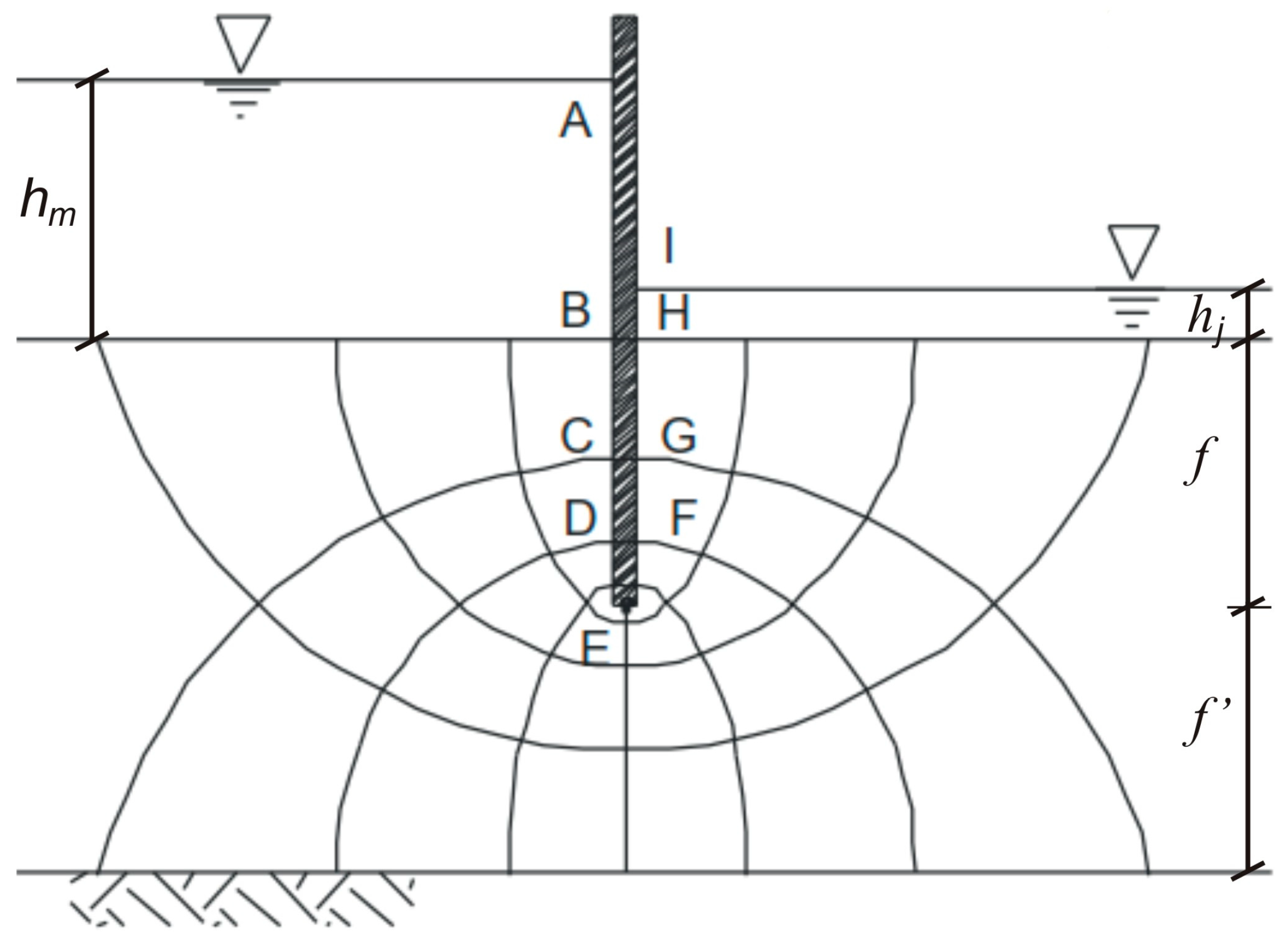
Figure 2.
Finite element mesh of the porous medium employing a sheet pile wall.
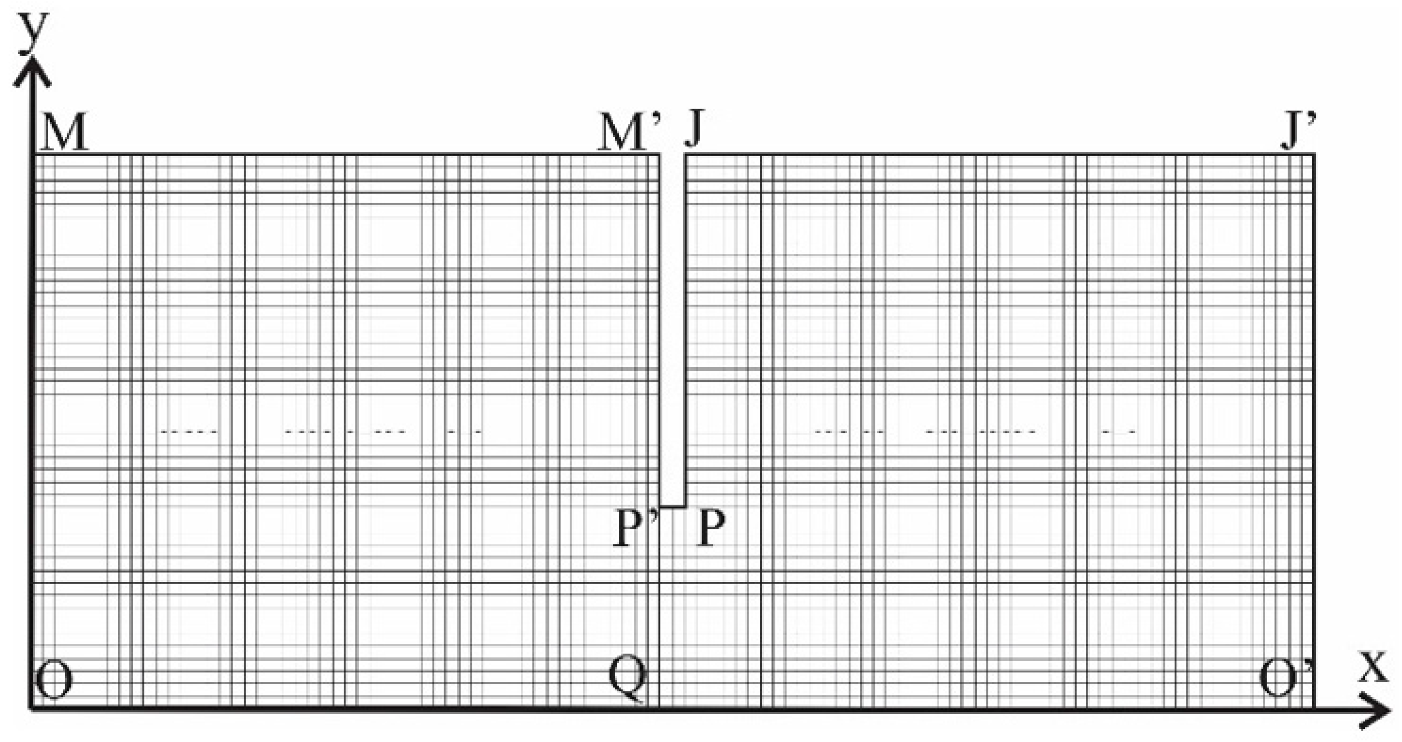
Figure 3.
Equipotential surfaces of the porous medium obtained using the MEF-D model.
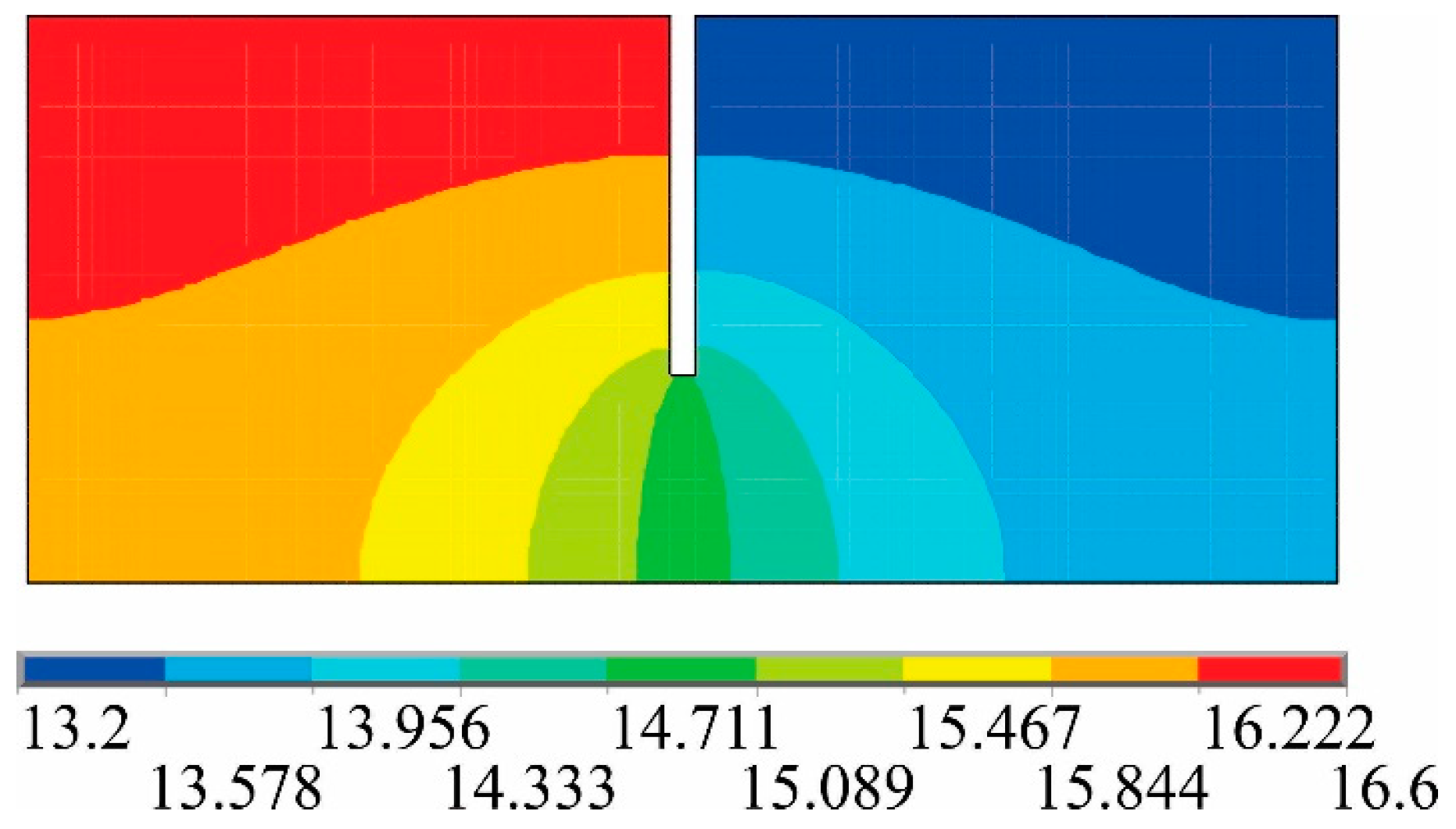
Figure 4.
Convergence analysis of the flow rate for the MEF-D model.
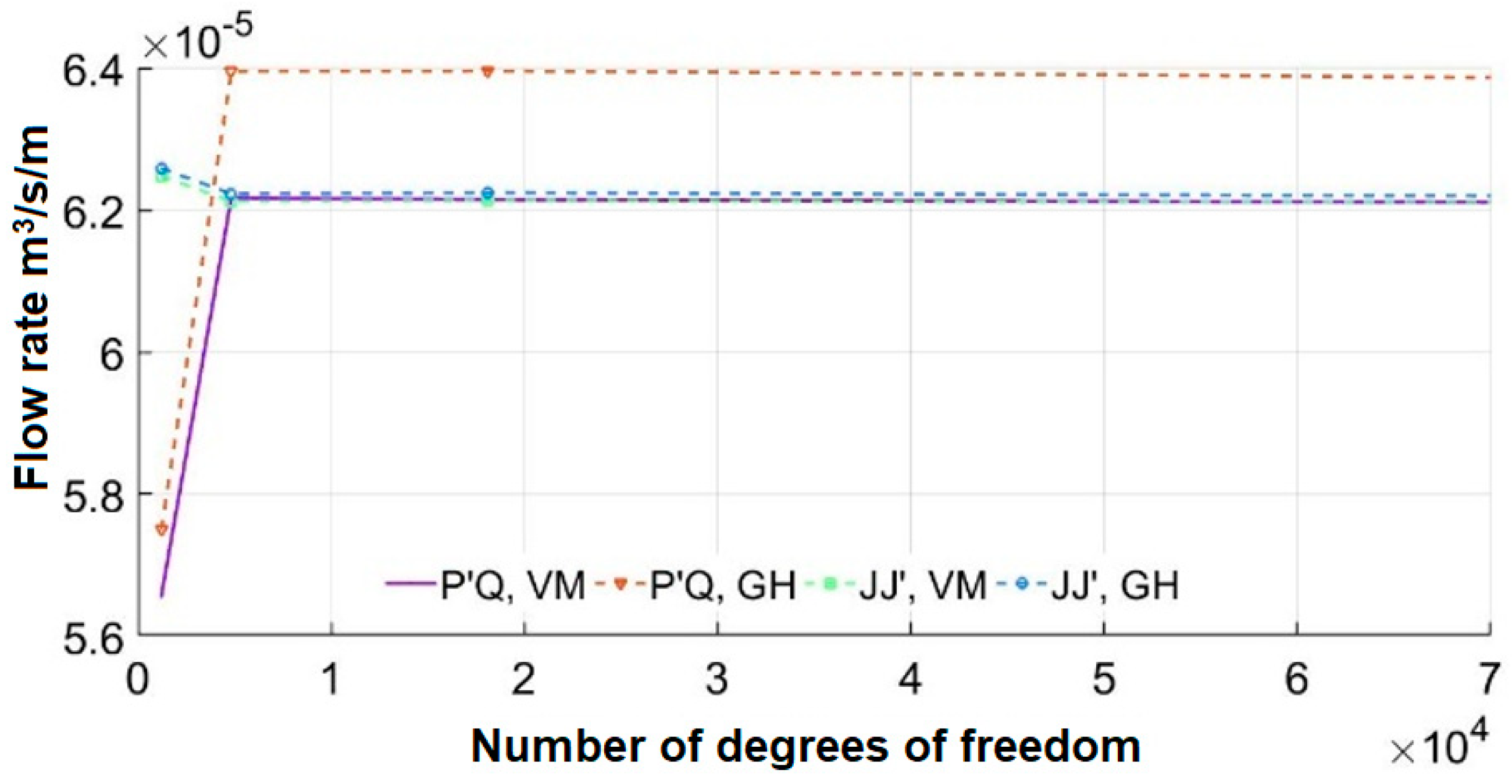
Figure 5.
Convergence analysis of the flow rate for the MEF-O model.
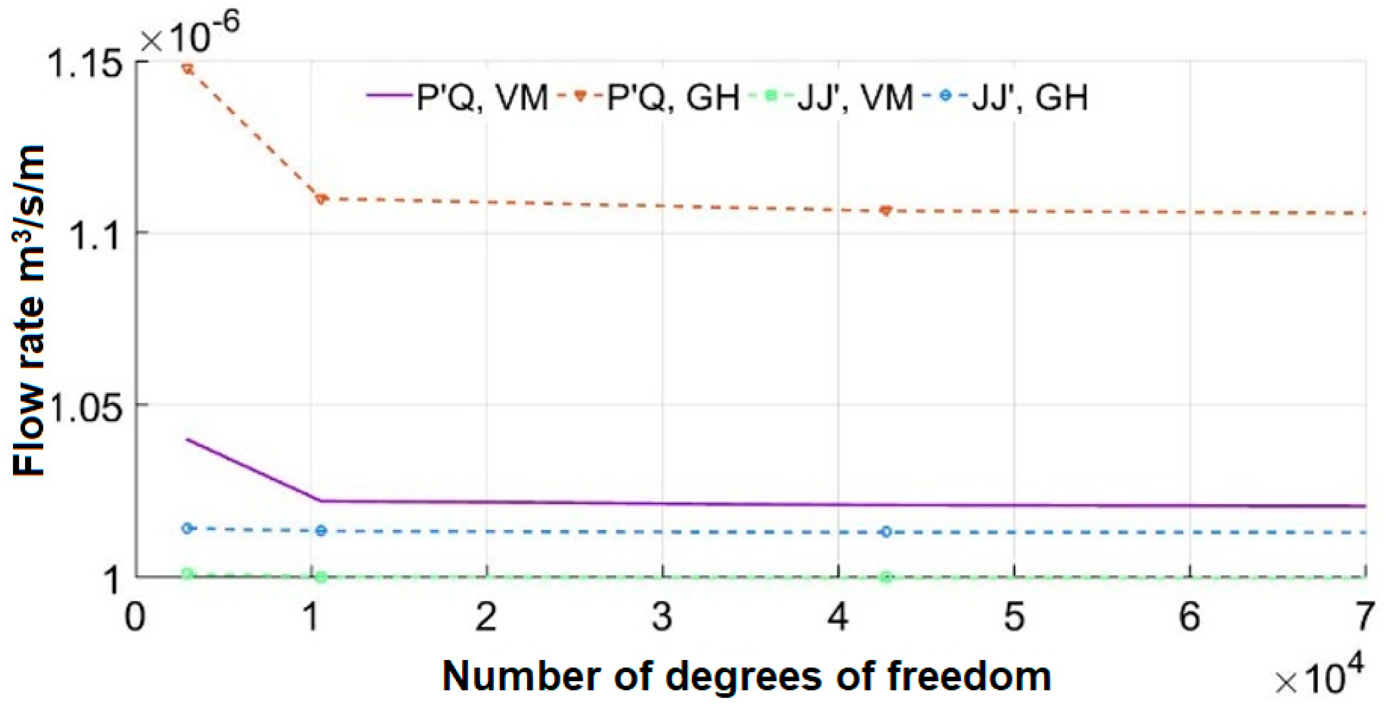
Figure 6.
Convergence analysis of the flow rate for the MEF-CS model.
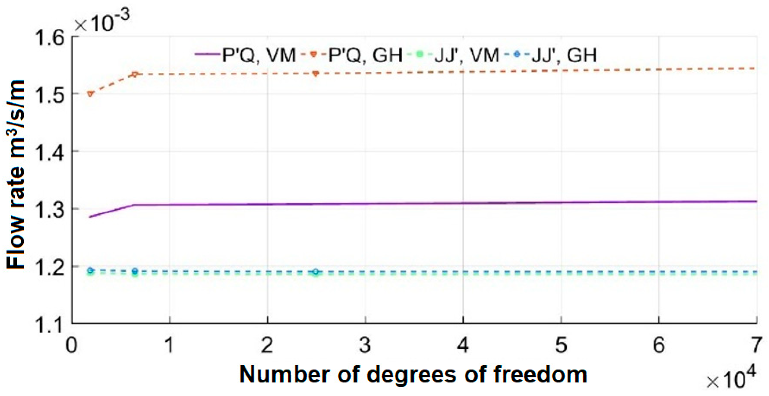
Figure 7.
Distribution of the resulting hydraulic gradient in the porous medium using the FEM-B containing elements: (a) of constant dimension, (b) more refined at the base of the sheet pile wall.
Figure 7.
Distribution of the resulting hydraulic gradient in the porous medium using the FEM-B containing elements: (a) of constant dimension, (b) more refined at the base of the sheet pile wall.
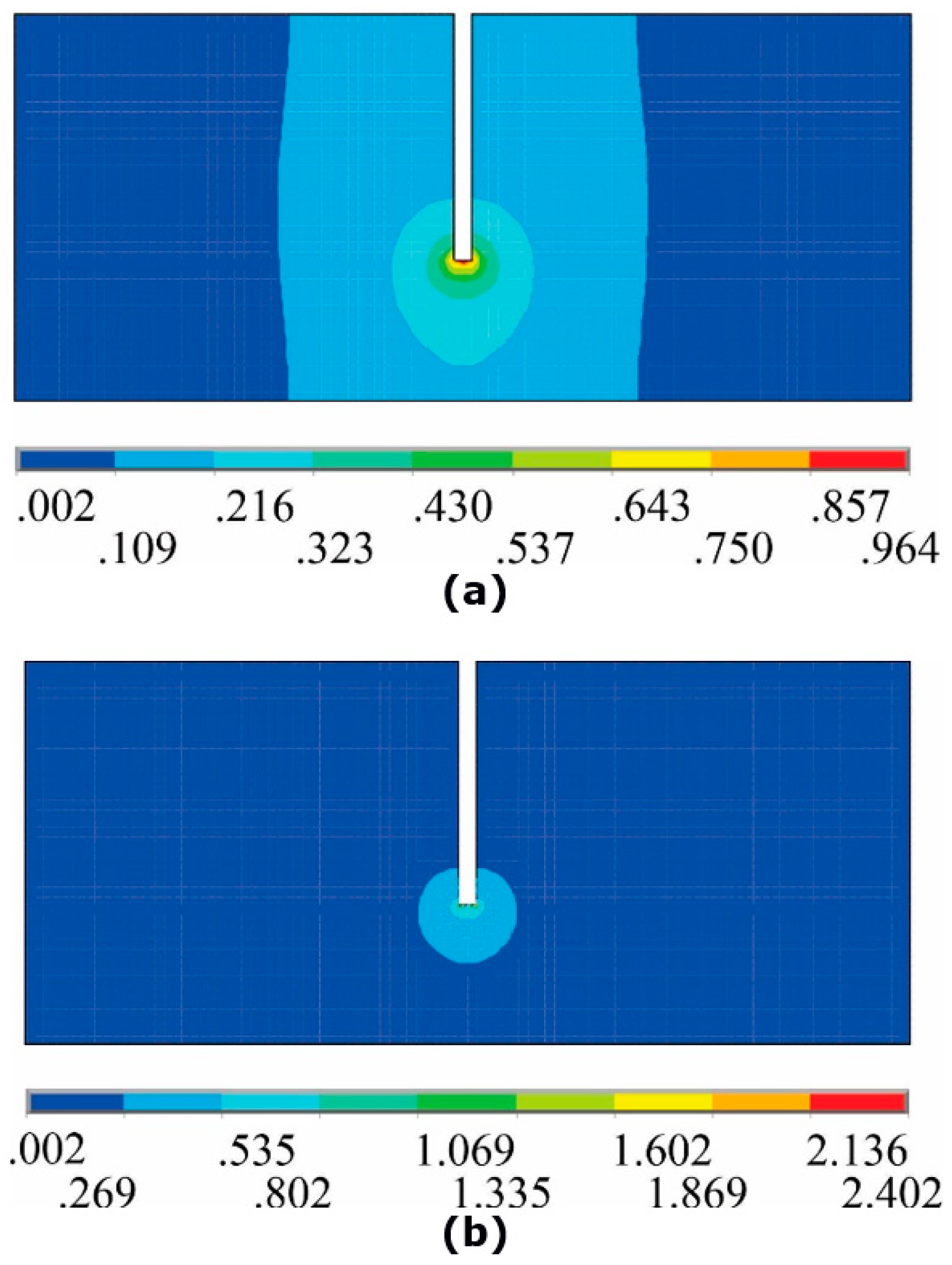
Figure 8.
Uplift pressures diagram along the upstream face of the sheet pile wall.
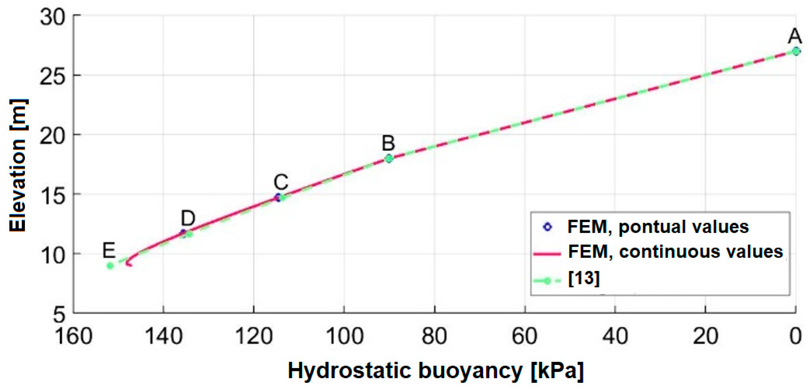
Figure 9.
Uplift pressures diagram along the downstream face of the sheet pile wall.
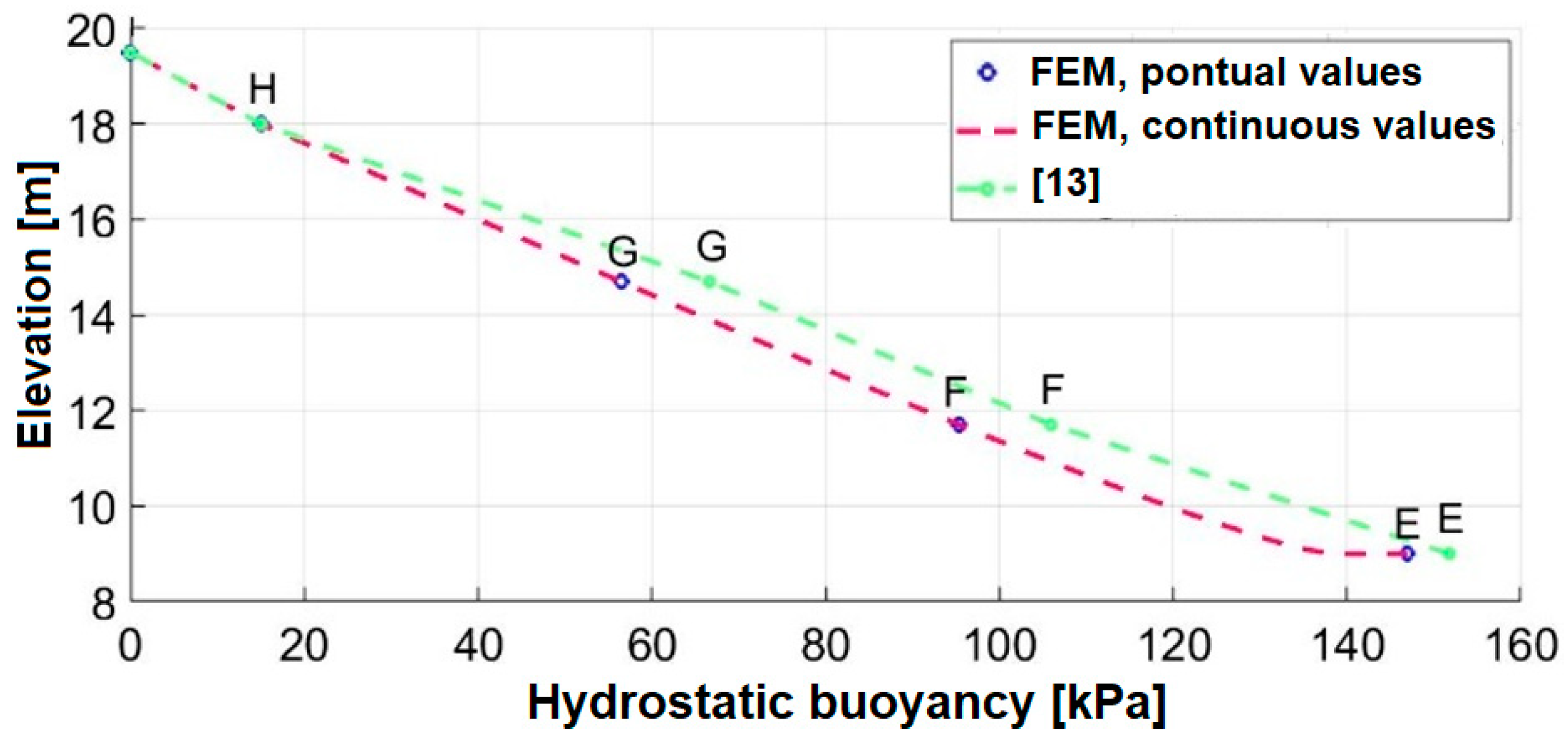
Figure 10.
Flow net under a gravity concrete dam resting on a porous medium (Adapted of [13]).
Figure 10.
Flow net under a gravity concrete dam resting on a porous medium (Adapted of [13]).
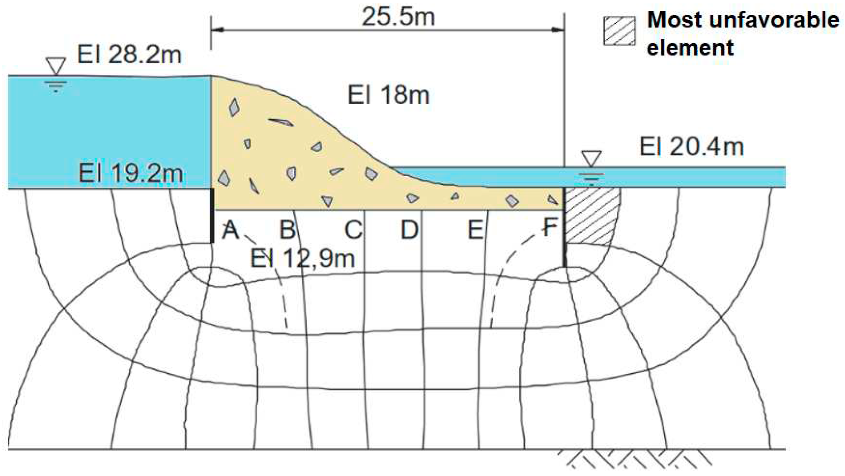
Figure 11.
Finite element mesh of the porous medium in a gravity concrete dam.
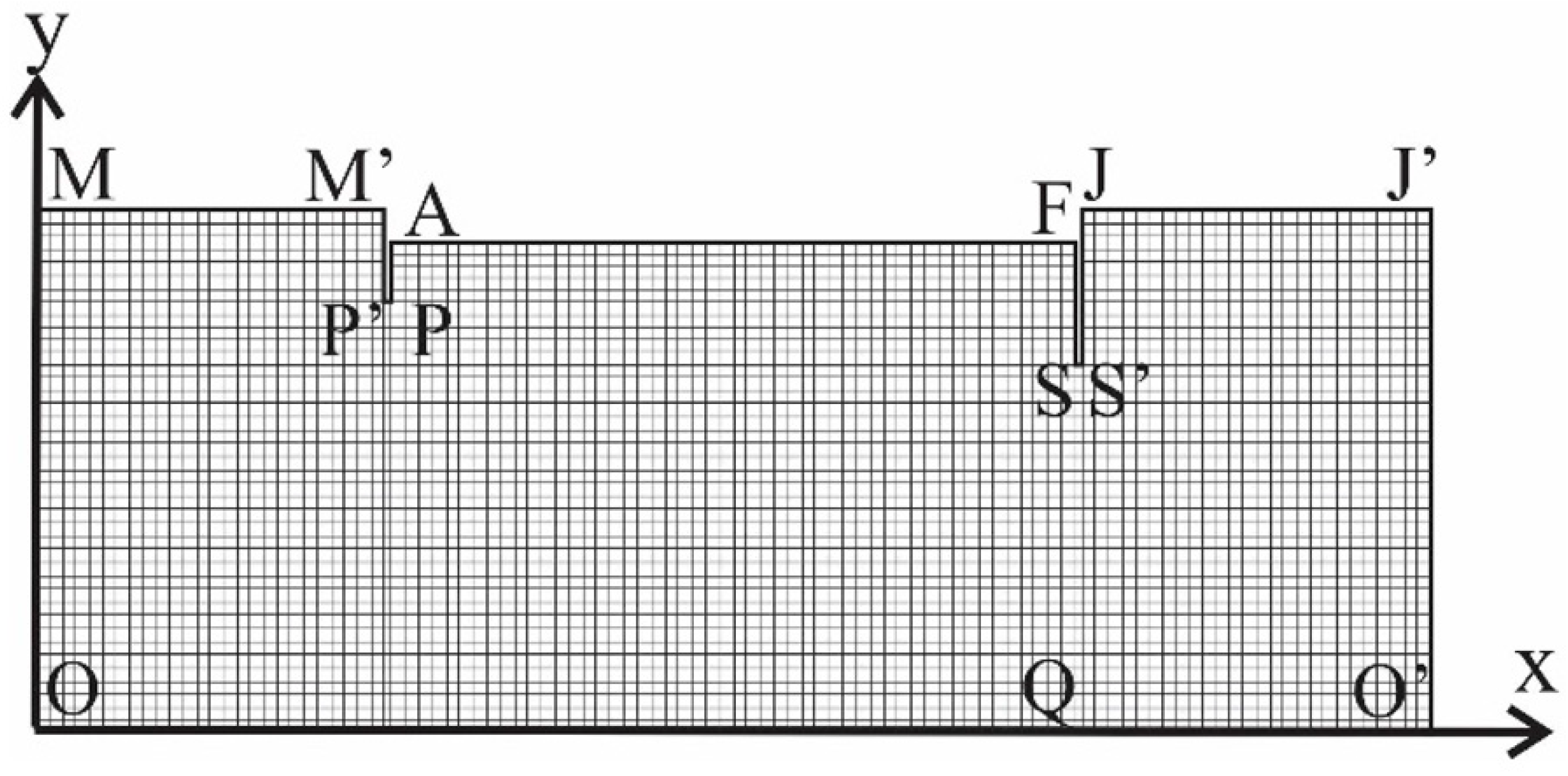
Figure 12.
Equipotential surfaces of the system modeled using Finite Element Method.
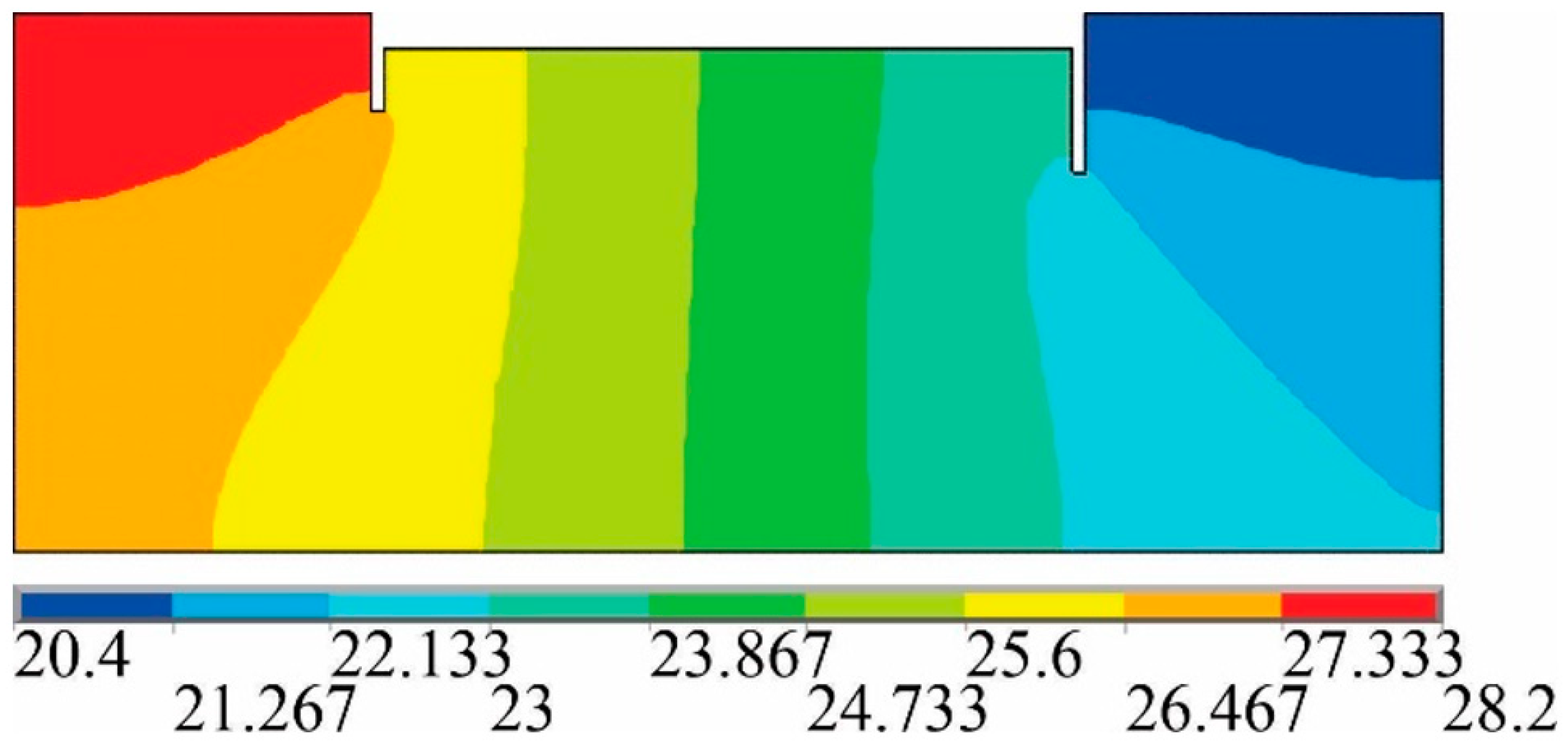
Figure 13.
Hydraulic gradient perpendicular to section SQ located between the base of the wall and the impermeable layer.
Figure 13.
Hydraulic gradient perpendicular to section SQ located between the base of the wall and the impermeable layer.
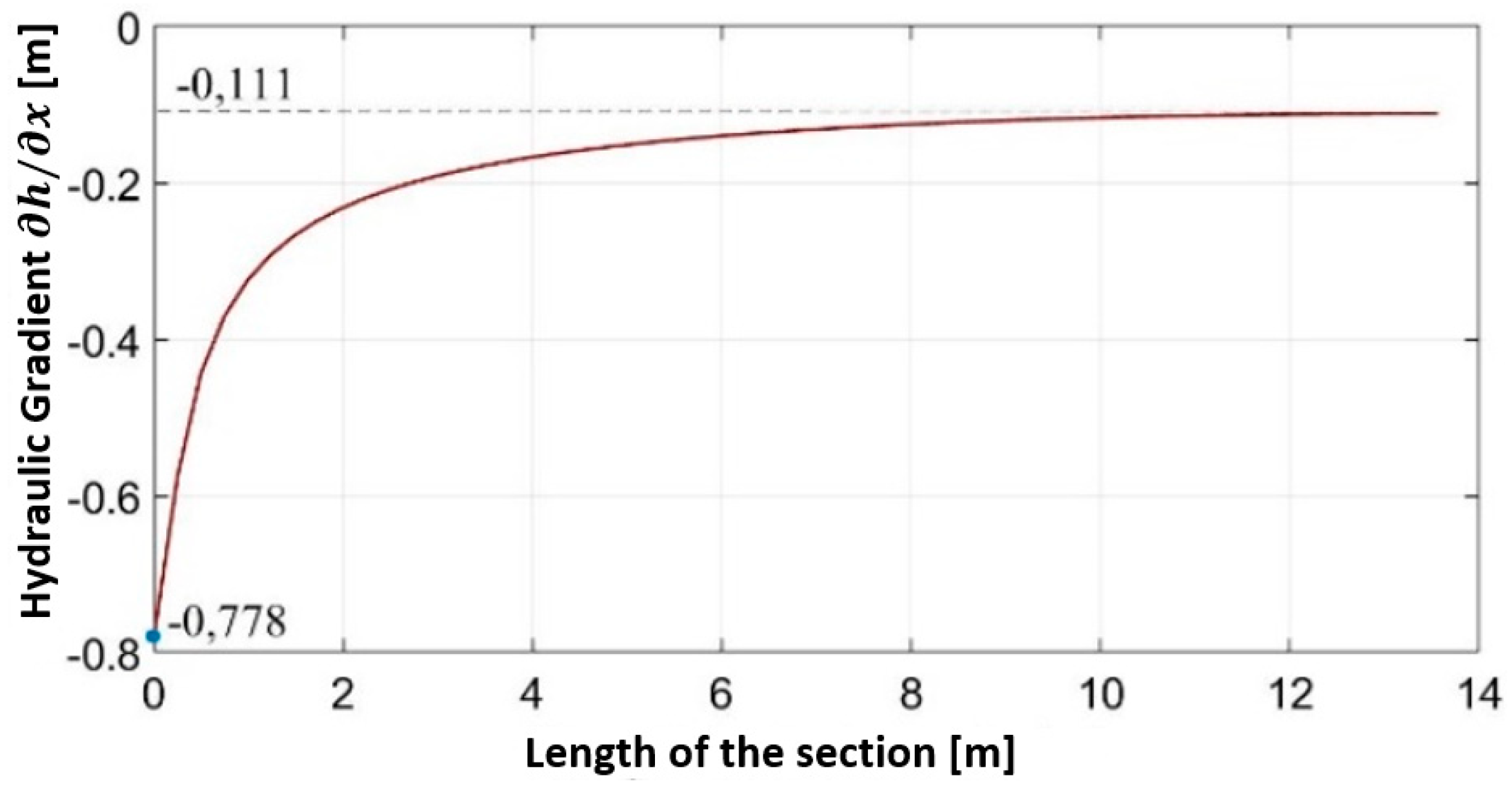
Figure 14.
Hydraulic gradient perpendicular to section JJ’ located downstream of the gravity concrete dam.
Figure 14.
Hydraulic gradient perpendicular to section JJ’ located downstream of the gravity concrete dam.
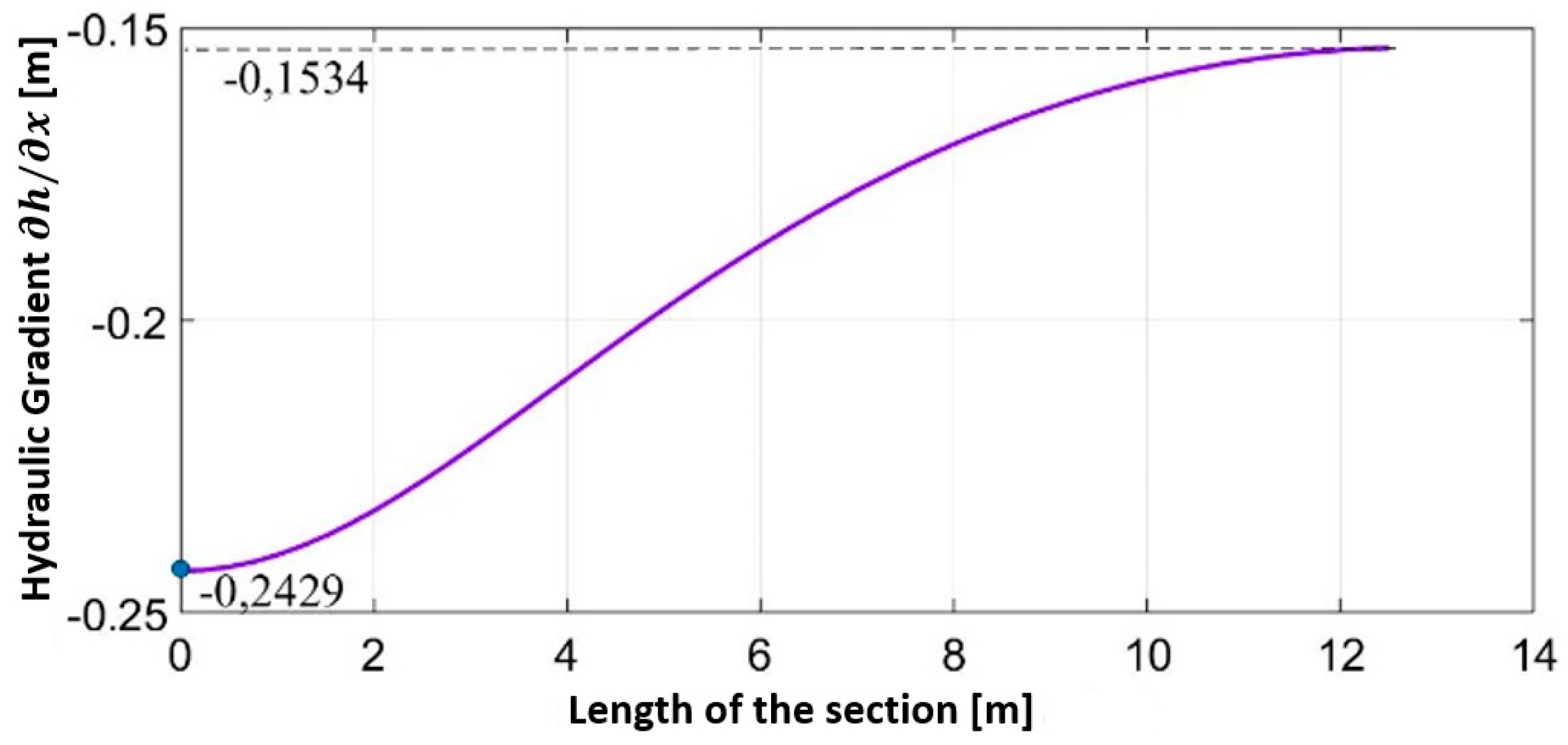
Figure 15.
Water pressure diagram under of the gravity concrete dam obtained via RF and FEM.
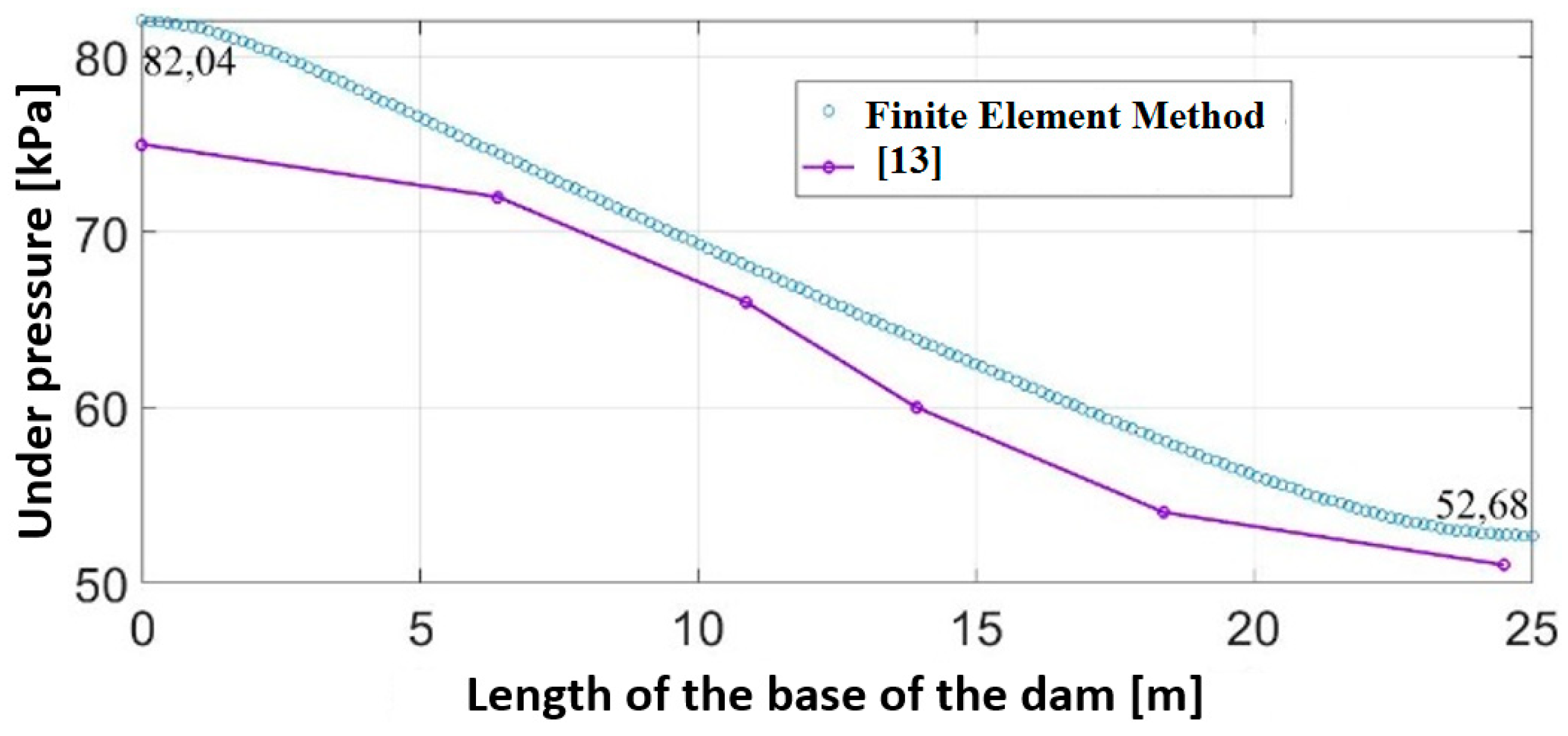

Table 1.
Hydraulic and geometric parameters of the porous medium and sheet pile wall.
| Parameter | Model of Finite Element | ||
|---|---|---|---|
| MEF-D | MEF-O | MEF-CS | |
| (m) | 5.6 | 9 | 25 |
| (m) | 2.2 | 1.5 | 0 |
| (m) | 3.4 | 7.5 | 25 |
| (m) | 7* | 9 | 25 |
| (m) | 11* | 18 | 50 |
| (m) | 0.5* | 0.3* | 0,3 |
| (m) | 25.5* | 35.7* | 120.3* |
| (m/s) | 5x10⁻⁵ | 3x10⁻⁷ | 1x10⁻⁴ |
*estimated values.
Table 2.
Flow rate in the porous medium considering different methodologies below a sheet pile wall (Flow rate unit: m3/s/m).
Table 2.
Flow rate in the porous medium considering different methodologies below a sheet pile wall (Flow rate unit: m3/s/m).
| Section | Methods and flow rate | Percentage difference | ||||
|---|---|---|---|---|---|---|
| RF (I) x10-5 | VM (II) x10-6 |
GH (III) x10-3 |
I-II I (%) |
I-III I (%) |
||
| [15] | P’Q | 6.74 | 6.217 | 6.395 | 7.760 | 5.119 |
| JJ’ | 6.212 | 6.222 | 7.834 | 7.685 | ||
| [13] | P’Q | 1.13 | 1.022 | 1.110 | 9.558 | 1.770 |
| JJ’ | 1.000 | 1.013 | 11.504 | 10.354 | ||
| [16] | P’Q | 1.25 | 1.368 | 1.534 | 9.440 | 22.720 |
| JJ’ | 1.187 | 1.191 | 5.040 | 4.720 | ||
Table 3.
Altimetric and total heads along the internal and external faces of the sheet pile wall using flow nets and FEM (I from [13] and II implemented using FEM).
Table 3.
Altimetric and total heads along the internal and external faces of the sheet pile wall using flow nets and FEM (I from [13] and II implemented using FEM).
| Point (x,y) (m) |
(m) |
(m) |
(m) |
Percentage Difference (%) |
|---|---|---|---|---|
| [I] | [II] | (I-II)/II | ||
| A (17.5; 9.0) | 27.00 | 27.00 | - | - |
| B (17.5; 0.0) | 18.00 | 27.00 | 27.00 | 0 |
| C (17.5;-3.3) | 14.70 | 26.06 | 26.158 | 0.38 |
| D (17.5;-6.3) | 11.70 | 25.12 | 25.264 | 0.57 |
| E (17.5;-9.0) | 9.00 | 24.18 | 23.695 | 2.01 |
| F (18.0;-6.3) | 11.70 | 22.30 | 21.236 | 4.77 |
| G (18.0;-3.3) | 14.70 | 21.36 | 20.342 | 4.77 |
| H (18.0; 0.0) | 18.00 | 19.50 | 19.50 | 0 |
| I (18.0; 1.5) | 19.50 | 19.50 | - | - |
Table 4.
Flow rate in the porous medium of a gravity concrete dam obtained considering different calculation methodologies (*[13]).
Table 4.
Flow rate in the porous medium of a gravity concrete dam obtained considering different calculation methodologies (*[13]).
| Section | Methods and flow rate x10-8 m3/s/m |
Percentage Difference (%) | |||
|---|---|---|---|---|---|
| RF (I) |
VM (II) |
GH (III) |
I-II I |
I-III I |
|
| SS’ | 1.200* | 1.193 | 1.219 | 0.583 | 1.583 |
| JJ’ | 1.200* | 1.214 | 1.217 | 1.167 | 1.417 |
Disclaimer/Publisher’s Note: The statements, opinions and data contained in all publications are solely those of the individual author(s) and contributor(s) and not of MDPI and/or the editor(s). MDPI and/or the editor(s) disclaim responsibility for any injury to people or property resulting from any ideas, methods, instructions or products referred to in the content. |
© 2023 by the authors. Licensee MDPI, Basel, Switzerland. This article is an open access article distributed under the terms and conditions of the Creative Commons Attribution (CC BY) license (http://creativecommons.org/licenses/by/4.0/).
Copyright: This open access article is published under a Creative Commons CC BY 4.0 license, which permit the free download, distribution, and reuse, provided that the author and preprint are cited in any reuse.