Submitted:
06 December 2023
Posted:
07 December 2023
You are already at the latest version
Abstract
This work explores five falling film evaporator (FFE) simulation approaches combined with energy consumption minimization strategies, namely Mechanical Vapor Recompression and Thermal Vapor Recompression (MVR and TVR respectively). Global system analysis and advanced dynamic optimization strategies are then investigated to minimize steam consumption, the cost of steam, the total annualized cost and maximizing product yield. The results indicate that a higher TVR discharge pressure, or MVR compression ratios, along with higher feed temperatures enhance evaporation with but increase operational costs. The most economic option includes three evaporator effects with TVR for achieving 50% product dry mass content. However, for a 35% dry mass content, MVR becomes cost-effective with an 11% reduction in unit electricity prices or a simultaneous 7% drop in electricity prices and a 5% increase in gas-based steam prices. Furthermore, switching from milk powder production to milk concentrates, an annual cost reduction ranging from 10.75 to 44% is achieved. Also, a forecasted 20% (or more) reduction of biomass-based steam cost can lead to lower annual expenditure comparing with the nominal NG-based steam Case. Regarding the total annualized cost, for a new plant design, optimization strategies lead to a 9 - 45% reduction in the total cost depending on the Case under consideration.
Keywords:
Milk industry
; Falling film evaporator
; Thermal vapor recompression
; Mechanical vapor recompression
; Dynamic optimization
; Global system analysis.
1. Introduction
Evaporation involves the conversion of a solvent into vapor, which is then removed from a solution or slurry. In most cases, water is the solvent used in evaporation systems. This process entails vaporizing a portion of the solvent to create a concentrated solution, thick liquor, or slurry [1].
Dairy manufacturers commonly employ concentration techniques to produce dairy products with higher levels of dry matter, increased value, reduced volume, and extended shelf-life [2]. Lowering the water activity and reducing transportation and storage costs are key benefits of dehydrating dairy products. This process involves converting a liquid product into a dry powder by removing nearly all the available water. However, dairy products are sensitive to heat, and their functional properties and digestibility can be negatively affected by excessive heat during the dehydration process. Therefore, a single water removal method cannot consistently achieve optimal performance. It thus, becomes necessary to employ multiple processing steps tailored to the specific properties of the material being processed, while considering both product quality considerations and processing costs [3].
Typically, the main steps involved in the production of milk powder include standardisation, homogenisation, pasteurisation, evaporation and drying [4]. Evaporation is a significant step in milk-powder production plants, serving not only to concentrate milk to the desired viscosity for subsequent spray drying but also to reduce the energy requirements during the spray drying process. In the evaporation stage, sterilized milk is concentrated under vacuum conditions at temperatures ranging from 40 to 70°C. This process leads to a significant increase in the total solids content, which typically rises from around 13% to 50% [5]. Vacuum conditions are used to mitigate the negative effects of heat on heat-sensitive milk components like fats and to prevent the degradation of essential nutrients, such as vitamins.
Milk powder production consists of many thermal processes, including evaporation and drying, and is responsible for 15% of the total energy use in the dairy industry [4]. In France, approximately 25% of the total energy consumption in food industry is attributed to the dairy sector [3]. Therefore, energy consumption attributed to the process of evaporation has a substantial impact on the cost of milk powder production.
To this end, there are several energy consumption optimization strategies in the evaporation of milk that have been discussed in the literature. The ones that are examined in this work involve the most commonly used in the industrial practice, such as the Mechanical Vapor Recompression (MVR) and the Thermal Vapor Recompression (TVR) technologies.
- In the evaporator unit, the excess heat generated by the secondary steam from the evaporator is typically released as waste heat. However, this waste heat can be effectively utilized to preheat the feed. An important feature of MVR technology is the utilization of the secondary steam cycle. MVR employs a mechanical fan, typically powered by electricity, to recompress low-pressure vapor to a slightly higher pressure and temperature.
- On the other hand, TVR utilizes a thermos-compressor, which employs high-pressure vapor to recompress low-pressure vapor to a slightly higher pressure and temperature. Numerous studies have demonstrated that multi-effect evaporation reduces energy consumption costs by enhancing steam economy. This is achieved by utilizing the secondary steam generated by the preceding effect as the heat source for the subsequent effect [6].
Jebson and Chen [7] assessed the effectiveness of falling film evaporators used in the New Zealand dairy sector for concentrating whole milk by calculating the kg steam utilized to kg water evaporated ratio and the heat transfer coefficient of each evaporator pass. The steam consumption of full and skim milk was comparable. Schuck et al. [3] introduced a methodology for assessing and comparing the energy consumption involved in the production of dairy and feed powders at various stages of the dehydration process. The findings of the study revealed that the energy consumption for fat-filled and demineralized whey powders were 9.072 kJ/kg and 15.120 kJ/kg, respectively.
Walmsley et al. [8] conducted a study on applying Pinch Analysis to an industrial milk evaporator case study to quantify the potential energy savings. By the appropriate placement of mechanical vapor recompression in a new improved two-effect milk evaporation system design, a 78% reduction to steam (6397 kW) at the expense of 16% (364 kW) more electricity use was achieved and the emissions reduction was 3416 t CO2-e/y. Srinivasan et al. [9] studied the energy efficiency at India’s largest milk processing plant and proposed retrofits for improving the plant’s sustainability. The results reveal that exergy efficiency of certain units is very low (<20%) while significant improvements in energy efficiencies can be achieved through simple, low-cost retrofits to these units. Moejes [4] studied the possibilities of upcoming milk processing technologies such as membrane distillation, monodisperse-droplet drying, air dehumidification, radio frequency heating, and radio frequency heating paired with renewable energy sources such as solar thermal systems. It was illustrated that the combination of developing technologies has the potential to cut operational energy consumption for milk powder manufacturing by up to 60%.
Zhang et al. [10] conducted a study by simulating a "pseudo" milk composition using hypothetical components in a commercial process simulator. The purpose of their work was to model a falling film evaporator commonly (FFE) employed in milk powder production plants. The study demonstrated that commercial process simulators have the ability to accurately simulate dairy processes. Building upon this research, Munir et al. [11] further enhanced the capabilities of commercial process simulators, providing valuable insights for practicing engineers to identify potential process improvements in the dairy industry. Bojnourd et al. [12] developed two types of dynamic models for an industrial four-effect falling-film evaporator used to condense whole milk: lumped and distributed. The findings indicate that while the distributed model demonstrates slightly better predictive capabilities compared to the lumped model, the latter outshines in terms of performance due to its simpler structure and significantly reduced simulation time. Zhang et al. [5] developed models for two commonly used types of milk powder evaporators: a conventional five-effect FFE without MVR and a three-effect evaporator with MVR. Heat-recovery processes were incorporated into the models to enable a comparison of energy consumption between the two processes. The results revealed that a three-effect FFE with MVR could achieve a 60% reduction in energy consumption compared to a conventional five-effect evaporator.
Gourdon and Mura [13] created a modeling tool based on experimental correlations built at industrial scale circumstances. The complicated interaction between the generated vapor and the liquid flow is included in their model. The results show that pressure drop is important in evaporator performance because of its influence on saturation temperature. Daz-Ovalle et al. [14] provided a set of dynamic models to study fouling of falling-film evaporators by considering fouling thickness, film thickness, temperature, and solids mass percentage. Hu et al. [15] developed a model for a water-to-water FFE simulation, which was employed in water vapor heat pump systems. That study focused on an existing FFE with four working tubes.
Bouman et al. [16] conducted experiments with a one-tube evaporator using whole and skim milk to ascertain the heat transfer and pressure decrease in evaporator tubes. Based on the findings, a computer software was created to optimize the design of multistage falling-film evaporators for dairy products. Silveira et al. [17] investigated the evaporation of water and skim milk using a pilot-scale, single-stage falling-film evaporator. In comparison to water, a thicker and slower film was formed at the end of the skim milk concentration procedure. They concluded that the behavior of a product during the evaporation process cannot be predicted solely by the overall heat transfer coefficient, and that a wide range of information, such as residence time distribution, product viscosity, and surface tension, is required to understand the evaporation process. Gourdon et al. [18] examined the flow behavior of a dairy product under falling film evaporation. The effects of varying dry solids concentrations, flow rates, and driving temperature changes were investigated. All three factors were shown to have a significant impact on the flow characteristics. Mura et al. [19] investigated the absolute vapor flow pressure losses during dairy product falling film evaporation using an experimental internal tube evaporator setup, adjusting the co-flow input velocity and product dry solid content. They concluded that pressure losses are strongly dependent on the co-flowing vapor rate for dry solid content between 13 and 40%.
Wijck et al. [20] conducted an evaluation of tools used for dynamic modeling and supervisory multivariable control design of multiple-effect falling-film evaporators. They specifically focused on the NIZO four-effect evaporator as a case study. The research aimed to achieve improved process operation for industries, leading to economic benefits such as increased yield, enhanced product quality, reduced energy consumption, and minimized material waste. Sharma et al. [21] created an Excel-based multi-objective optimization tool based on the elitist non-dominated sorting genetic algorithm (NSGA-II) and tested it on benchmark tasks. It is then used for multi-objective optimization (MOO) of the design of a falling-film evaporator system for milk concentration, which includes a pre-heater, evaporator, vapor condenser, and steam jet ejector. Haasbroek et al. [22], conducted a study utilizing historical data from a FFE to develop models for control purposes, without requiring knowledge of the plant's physical dimensions. The results indicated that fuzzy predictive controllers and LQR control exhibited the highest performance, followed by cascade control, and finally, PI control. Galvản-Ángeles et al. [23] analyzed a thermo-compression evaporation method for milk. The suggested tool considers the cost optimization of the evaporation system while incorporating thermo-physical parameters of the foodstuff as a function of composition and temperature. The results revealed that the evaporation economy is proportional to the percentage of recycled steam and the location of the effect that recycles the steam, and inverse to the thermodynamic efficiency of the thermo-compressor.
This work aims at optimizing the milk evaporation process by minimizing steam consumption under the operational and product quality constraints. To this end, 5 different Cases of evaporator layouts are examined using a global system analysis (GSA) and an advanced optimization approach. GSA is employed to revise decisions to improve system robustness, validate the process and reduce parameter uncertainty. An uncertainty analysis allowed the investigation of the impact of design and operational decisions and environmental inputs on Key Performance Indicators (KPIs). Afterwards, Cases 1-4 are optimized under 5 different scenarios, either minimizing the cost of steam while maximizing product yield or minimizing the total annualized cost which is applicable to a new plant design or a capacity expansion option. Steam economy, energy consumption profile and heat transfer areas are assessed and compared. Moreover, this study investigates to what extend switching from milk powders to new products known as milk concentrates effects the energy consumption in the evaporation process. Thus, Cases 1-4 are optimized under different end-product specifications (30, 35 or 50% solid content). Finally, it is evaluated whether the use of MVR or TVR is more economical for the evaporation process, based on current steam and electricity prices, economic trends, and costs of steam generated from renewable energy sources.
The remaining of the article is structured as follows: Section 2 describes the material composition along with some of its properties. Section 3 provides a detailed presentation of the mathematical model that describes the operation of a falling film evaporator. Sectio 4 presents the studied evaporator layouts. The attained global system analysis and optimization results of each studied Case/evaporator layout are presented and thoroughly discussed in Section 5. Finally, Section 6 summarizes the concluded remarks emerging from the study.
2. Materials
This section provides information about milk properties and conditions. In the present study, the analysis of FFEs is applied to the milk evaporator process, while the thermo-physical properties of the food vary with composition. Two different composition profiles of whole milk before evaporation are examined (Table 1) while Table 2 summarizes equations for the calculation of properties in the mixture. Thermodynamic and physical properties such as specific heat capacity , thermal conductivity , and density, , of ‘pseudo’ milk are modelled using the process simulator and average values are compared to the literature. The results are summarized in Table 3.
3. Process model
The concentration of milk in this study is focused on falling film evaporators. In this process, the milk, which is close to its boiling point, is introduced in a uniform manner at the upper section of the inner surface of a tube. These tubes are arranged side by side, fixed in place, and surrounded by a jacket. As the milk descends within each tube, it forms a thin film and undergoes boiling as a result of the heat exchanged with the steam. The concentrated liquid is collected at the lower part of the equipment, while the remaining portion is separated from the steam in a subsequent separator. In evaporators equipped with multiple effects, the concentrated liquid is pumped to the next stage, while the steam serves the purpose of heating the subsequent [2].
A dynamic model of a simple falling-film evaporator is developed in this Section. The model examines the flash calculations of liquid entering the evaporator, its distribution through distributor plates, and its evaporation as it flows downwards through pipes. The model has been developed based on the following assumptions:
- It is assumed that the product immediately reaches its boiling temperature once it passes above the distributor plate, with either steam flashing or condensing.
- All the heating steam condenses at its saturation temperature. The heat released during condensation is utilized to preheat and evaporate the feed stream.
- The pressure difference on the steam side is insignificant, thus resulting in a constant temperature on the steam side.
- The unit is assumed to be perfectly mixed at all times, implying there are no spatial variations in intensive properties within it.
- A steady state balance is applied to the tube flow, but the mass hold-up of liquid on the distributed plate is calculated.
3.1. Mass balance
The rate of change of the mass hold-up, , of any given species in phase in the unit is given by Equation (4):
Where is the mass flowrate of the jth feed stream in phase p, is the mass fraction of species i in the jth feed stream in phase p, is the mass flowrate of material phase p in the outlet stream, is the mass fraction of species i in the outlet stream of phase p and is the rate of mass transfer between the phase p and the phase pn.
Assuming that the unit is perfectly mixed, the composition of any outlet stream is the same as the composition within the unit:
Where is the mass fraction of species i in phase p in the unit.
The composition of material within the unit is given by Equations (6),(7):
Where is the total holdup of material in phase p within the unit.
3.2. Energy balance
The rate of accumulation of enthalpy, , within the unit is given by Equations (8),(9):
Where is the specific enthalpy of the material in the unit in phase p, is the specific enthalpy of the jth feed stream in phase p, is the specific enthalpy of the outlet stream in phase p, is the enthalpy of phase change between phase p and phase pn and is the enthalpy transferred into the unit through boundary due to heat loss, heating and so forth.
Due to the assumption that the unit is perfectly mixed, the specific enthalpy of each of the outlet streams is equal to the specific enthalpy of the material within the unit:
The specific enthalpy is assumed to be a function of the composition and temperature, , of the material within the unit:
3.3. Heat transfer rates
The total heat transfer rate, , is the sum of energy transfer by steam, and energy loss, , to the environment:
Where is the overall heat transfer coefficient, is the heat transfer area, is the number of tubes, is the length of the tubes and finally and are the linear and logarithmic temperature differences, respectively.
3.4. Flow through distribute plate
The distribute plate is an inserted plate that distributes product stream evenly around the inner periphery of the evaporator tubes. Aside from the liquid holes that allow liquid to pass through, there are also openings to let steam flow through the plate. Two designs for vapor transport through the distribute plate are considered:
- Plate with upstanding vapor tubes.
- Plate with an upstanding rim at the edges of the circular plate and a ring-shaped gap between plate and evaporator body.
The vapor flowing downwards or upwards through the distribute plate causes a vapor pressure drop, while the liquid flowing downwards through the distribute plate and liquid holdup above the plate cause a liquid pressure drop.
The vapor flow through plate, , for plate design with upstanding vapor tubes is expressed by the following relation.
Where is the number of vapour uprising tubes, is the diameter of each uprising tube, is the length of each tube, is the vapor density above plate, is the vapor friction factor and is the vapor pressure drop.
The vapor flow through plate for plate design with upstanding rim at the edges is expressed by Equations (18)-(19):
Where are the diameter of the evaporator body and the plate respectively and is the height of the outer rim.
The liquid flow through plate, , is expressed by Equations (20)-(21):
Where is the number of liquid holes, is the diameter of liquid holes, is the thickness of the distribute plate, is the liquid density above plate, is the liquid flow velocity through plate, is the liquid friction factor and is the liquid pressure drop.
3.5. Liquid flow through pipes
The wetting rate, , of a falling film evaporator tube is correlated to the liquid mass flow of the tube, and the tube diameter through:
The Reynolds number,, in the falling film evaporation used in empirical relations is defined by Equation (23):
Where is the liquid dynamic viscosity.
The liquid characteristic length, , is given as:
Where is the liquid density and is the gravity acceleration.
The film thickness, , is calculated by Equation (25):
Assuming that the film thickness is small compared to the tube diameter, the liquid velocity downwards on the tube, , and the residence time, , for liquid flow to the bottom are calculated based on Equations (26)-(27):
3.6. Boiling point elevation
The boiling point elevation of a solution can be calculated by combining the laws of Raoult and Clausius Clapeyron:
Where is the gas constant, is the boiling temperature of water, is heat of evaporation, is molar weight and is the molar fraction of water in the solution.
It is assumed that fat does not dissolve in the solvent and therefore does not affect the boiling point. The molar fraction of water in the fat-free product can therefore be calculated:
Where denotes for the mass fraction and refers to all but fat components.
3.7. Liquid friction factor
The most widely used correlations for liquid friction factor is the Wallis correlation for annular falling film and it is incorporated to the model for better prediction of the liquid friction factor [19].
3.8. Energy cost
In order to compare the energy consumption of TVR and MVR, the variable Energy cost is used, defined by Equation (31). When employing TVR technology, the annual cost is given as:
For MVR technology, the annual energy cost is expressed as:
4. Case Studies
Five different evaporators are considered, combined with different energy consumption minimization strategies, namely MVR and TVR. These process alternatives are often met in the food processing industry. A brief description of each studied Case is given below, while the corresponding falling film evaporator layouts is showed in Figure 1. The design characteristics of the evaporators of each layout are provided in Tables S1–S4 of the Supplementary material.
Cases 1 and 5 represent industrial scale evaporator systems while Cases 2,3 and 4 are related to pilot conditions (1,000 kg/h).
4.1. Case 1
4.2. Case 2
Raw milk enters the preheater tubes of the 2nd and the 1st evaporator tubes before entering the 1st evaporator chamber, as shown in Figure 1(b). As the evaporation process continues in FFE1, the generated steam works as the heating medium in the 2nd evaporator effect where the semi-concentrated product is further evaporated resulting to end-product (concentrate). The steam generated in the 2nd effect is recycled to TVR where fresh steam is added, increasing its pressure before entering the 1st effect.
4.3. Case 3
In Case 3, 1,000 kg/h raw milk are fed to the preheater tubes of the 3rd, 2nd, and 1st evaporator effect subsequently, before entering the 1st evaporator chamber, as shown in Figure 1(c). As the evaporation process continues in FFE1 and FFE2, the generated steam at each effect works as the heating medium for the next one, and the whole process results to end-product (concentrate). The steam generated in the 3rd effect is recycled to TVR where fresh steam is added, increasing its pressure before entering the 1st effect.
4.4. Case 4
In Case 4 (Figure 1(d)), 1,000 kg/h raw milk are fed in a single-stage evaporator, with no addition of external steam. The evaporation occurs only by recompressing the vapor generated and recycling it to the unit by an MVR. The only source of energy needed in this process is electricity.
4.5. Case 5
Case 5, presented in Figure 1(e), examines the proposed evaporation system by Galvản-Ángeles et al. [23] and it has four effects with co-current flow, capable of processing 16,000 kg/h of whole milk. The arrangement employs TVR technology, recycling vapor from the 2nd to the 1st stage of evaporation.
5. Results
5.1. Solution method
In the present study, global system analysis and optimization were conducted in gPROMSTM FormulatedProducts [28] version 2.3.0 from Siemens Process Systems Enterprise. A database containing physical and thermodynamic properties of milk components was developed using gPROMS FormulatedProducts Utilities.
5.2. Global system analysis (GSA)
GSA allows for a systematic exploration of the relative impact of input parameters on model output responses. The fundamental principle of GSA involves sampling from a defined particulate system. This entails extracting various values for individual parameters and calculating the corresponding output values.
Uncertainty analysis, can be conducted using the Monte Carlo method, is employed to determine the effects of uncertain input parameters on the system responses. The Monte Carlo method involves performing multiple model evaluations using either deterministic or probabilistic distributions. The resulting output values from these evaluations are then utilized to assess the impact of system's uncertainty. In this study, uncertainty analysis was conducted to assess key decision space optimal areas rather than single optimal values of the degrees of freedom. Uncertainty analysis was performed for all Cases, implementing standard Monte Carlo method. Quasi-random (Sobol) sampling was used as the sample generation method which fills the space uniformly and it is proved efficient for medium-sized problems and a high number of samples. The number of uncertainty scenarios is set to 1000.
5.2.1. Steam cost analysis
This study also considers the uncertainty of steam price. Steam can be generated from a wide range of sources, including fossil fuels such as natural gas (main source), as well as renewable energy sources like lignocellulosic biomass, solar and waste. The rise of renewable energy sources presents an opportunity to examine the prices of steam generated from these sources, taking into account their future values, which could potentially fluctuate by around ±40%. Pérez-Uresti et al. [25] evaluated the production cost of renewable-based steam including solar, lignocellulosic biomass and biogas. Results showed that, considering the current price of steam based on NG, lignocellulosic biomass offers better perspectives to become a competitive resource when compared to the other two sources. More specifically, the evaluated production cost of steam are as follows: NG-based steam costs 16.81 $/tn, biomass-based steam costs 20.37 $/tn, solar based steam costs 32.5$/tn and for biogas-based steam costs 27.42 $/tn.
The analysis conducted in this work takes into account future values of those described above, which could potentially fluctuate by a maximum of 40%, to determine to what extent and in what circumstances renewable-based steam can become a competitive resource compared to natural gas. The specific analysis involves only Case 1, because the same pattern of results would emerge when investigating the rest of the Cases.
Table 4 summarizes the prices examined, to determine to what extent and in what circumstances renewable-based steam can become a competitive resource compared to natural gas.
Uncertainty analysis results related to operating annual cost of evaporation depending on various steam sources and future steam unit costs are summarized in Table 5, which provide a detailed comparison and assessment of steam sources. Despite natural gas being currently the most economical choice, a future possible reduction of biomass-based steam cost by only 20% (or more) would lead to lower values of annual expenditure for the evaporation process of Case 1, compared to the nominal scenario of using NG-based steam. Solar-based steam and biogas-based steam do not seem economically attractive after the analysis as reduction of 40% for the former or over 50% for the latter would be needed in order for those sources to be competitive to natural gas. However, as predictions indicate a rise in natural gas’ price, renewable-based steam would become more and more competitive both for environmental and economic reasons.
5.2.2. GSA-Case 1
The factors used for the uncertainty analysis for Case 1 are the steam cost, the TVR discharge pressure, the TVR suction ratio, , (given as SR = Steam mass flowrate (suction)/ Steam mass flowrate (motive)), and the feed temperature. The lower and upper bounds along with the probability distribution of the factors are presented in Table S5 of the Supplementary material.
Figure 2(a) illustrates the variation of concentrate mass fraction of water versus feed temperature and TVR discharge pressure. It is clear that higher outlet pressures and higher feed temperatures result to a lower mass fraction of water in the end product, thus, leading to a product with higher dry mass fraction. Higher feed temperatures can be achieved by preheating the feed stream.
As shown in Figure 2(b), the TVR suction ratio illustrates the largest effect on the steam economy. The steam economy is defined as sum of the vapor mass flowrate of each evaporator effect i divided by the feed mass flowrate (Steam economy=Total mass flowrate of evaporated water(kg/h)/Fresh steam mass flowrate (kg/h)). Suction ratios over 1.3 results to higher values of yield, while high feed temperatures along with suction ratios over 1.6 can result to a steam economy close to 4. On the contrary, motive steam mass flowrate is mostly affected by TVR discharge pressure, as shown in Figure 2(c). Low values of discharge pressure result to minimum mass flowrates (around 600 kg/h steam) whereas high outlet pressures along with low suction ratios can result to even 3200 kg/h steam which quintuple cost of evaporation.
From Figure 2(d) and Figure 2(e) it can be seen that TVR discharge pressure affects both the pressure of concentrate product and the solid mass fraction of the FFE1 outlet product. Higher discharge pressure values can be mutually beneficial both for achieving greater vacuum (lower concentrate pressure) and resulting to more concentrated products (lower moisture content) which is ideal for downstream spray drying processes.
5.2.3. GSA-Case 2
Uncertainty analysis was performed for Case 2 to examine the effect of key factors on various key responses (model variables). The factors of this analysis are the TVR discharge pressure, the TVR suction ratio and the feed temperature. information about the factors of this Case is provided in Table S6 of the Supplementary material.
As responses of several variables were discussed in the GSA of Case 1 which also includes two evaporator effects with TVR in plant scale, in this section it is worth highlighting differences in responses related to laboratory scale or responses of other important variables. From Figure 3(a) it can be seen that in laboratory scale, higher values of steam economy can be achieved as the lower and upper bounds of this variable are higher than that of Figure 2(b) (1.4 as opposed to 1 and 5.2 as opposed to 5 respectively).
Figure 3(b) illustrates that although the lower bounds of solid mass fraction after the first evaporation effect are the same as Figure 2(e) (plant scale), the upper bounds are remarkably higher (almost 0.45) indicating that a single evaporation effect would be sufficient in some cases depending on the underlying product specifications.
Figure 3(c) illustrates the annual cost of steam versus feed temperature and TVR outlet pressure. The steam unit cost is fixed at 20$/t (NG – based steam) while the operating hours are 7,920 h. The results show that the operating conditions can greatly affect the annual cost ranging from 6,000 to 44,000 $/year. However, these values are related to different end product specifications, so the final optimization results are presented in Section 4.2.
5.2.4. GSA-Case 3
Uncertainty analysis was also performed for Case 3. The factors used in this analysis are the same as Case 2.
Figure 4(a) shows the variation of steam economy versus feed temperature and suction ratio. It is demonstrated that an arrangement of 3 evaporator effects with TVR leads to high steam economy values compared to Case 2. Specifically, lower and upper bounds of steam economy in Case 3 are 2.5 and 7.5 respectively as opposed to 1.4 and 5.2 of Case 2. Figure 4(b) and Figure 4(c) illustrate the variation of dry mass fraction at FFE1 and FFE2 evaporator tubes outlet respectively, while Figure 4(d) shows the water mass fraction of the concentrate (end product). Higher values of TVR discharge pressure result to more concentrated products while FFE1 liquid product can have 13% to 18% solid content in Case 3 as opposed to 14% to 46% of that of Case 2. In Case 3, the maximum solid concentration of FFE2 outlet product is 26% which implies that the evaporation process is mainly enhanced in the 3rd effect, rather than the 1st one in the case of two evaporator effects with TVR (Case 2).
Figure 4(e) illustrates the annual cost of steam versus TVR suction ratio and TVR outlet pressure. The steam unit cost is fixed at 20$/t (NG – based steam) and the operating hours are 7,920. The results show that higher values of outlet pressure combined with low values of suction ratios can greatly increase the annual cost. On the other hand, Case 3 results to lower steam annual cost than that of Case 2. Specifically, the analysis of Case 2 resulted to operating costs of 6,000 – 44,000 $/year (Figure 4(c)) as opposed to 4,000 – 32,000 $/year of Case 3.
5.2.5. GSA-Case 4
The factors consided for the uncertainty analysis for Case 4 are the MVR compression ratio and the feed temperature. The compression ratio is expressed as: CR = Steam pressure (outlet)/ Steam pressure (inlet). The lower and upper bounds along with the probability distribution of the factors is provided in Table S7 of the Supplementary material. The results are shown using various figures, while TVR and MVR operation can be assessed and compared.
Figure 5(a) illustrates the moisture mass fraction of concentrate versus feed temperature and MVR compression ratio. Higher values of compression ratio and feed temperature result to more concentrated products and especially compression ratios over 1.25 lead to an efficient evaporation (solid mass fraction over 0.3). Consequently, the operating cost of evaporation as expressed by Equation (31b), rises with higher values of compression ratios (Figure 5(b)).
It is worth mentioning that the electricity unit cost is fixed at 0.21$/kWh and the operating hours are 7,920. The results show that the operating conditions can greatly affect the annual cost ranging from 2,000 to 36,000 $/year. Comparing with Cases 2 and 3, Case 4 leads to the lower minimum cost (2,000$/year as opposed to 4,000$/year and 6,000$/year of Cases 3 and 2 respectively) and an intermediate upper bound (36,000$/year as opposed to 32,000$/year and 44,000$/year of Cases 3 and 2 respectively). However, these values are related to different end product specifications and a comprehensive comparison is made using dynamic optimization techniques and results are presented in Section 5.3.
Finally, Figure 5(c) depicts the variation of concentrate product pressure versus MVR compression ratio and feed temperature. The latter one illustrates the greatest impact on the achieved vacuum, as lower values of feed temperature result to greater vacuum (around 2500 Pa pressure). However, as shown in Figure 5(c), end-product dry mass fraction over 0.5 cannot be achieved for feed temperatures lower than 40°C.
5.2.6. GSA-Case 5
Uncertainty analysis was finally performed for Case 5 to examine the effect of the split fraction, TVR suction ratio and feed temperature (factors) on various KPIs. More information about the studied factors is provided in Table S8 of the supplementary material. As Case 5 involves a plant scale process with 4 evaporator effects by recycling steam from the 2nd effect to TVR, different recycling fractions (split fractions) can be examined. Furthermore, both plant and laboratory processes can be evaluated.
Figure 6(a) illustrates the water mass fraction of concentrate product versus the feed temperature and split fraction. Empty spaces indicates that simulations cannot be provided in certain areas, thus, recycling over 60% of FFE2’s steam (providing FFE3 with the remainder steam) while keeping the feed temperature below 50°C results to failed simulations. However, higher feed temperature and lower split fractions enhance the evaporation process as the concentrated product has lower moisture content. This implies that by providing more steam to the next evaporator effect, the evaporation is more enhanced than recycling larger quantities of steam in the TVR unit.
Figure 6(b) shows the variation of yield versus the feed temperature and split fraction. The evaporation yield is defined as the mass flowrate of end product (concentrate) divided by the feed mass flowrate (Yield = Concentrate mass flowrate (kg/h)/Fresh steam mass flowrate (kg/h)). It follows the exact opposite pattern with Figure 6(a), as higher feed temperature and lower split fraction result to lower product yield. However, despite producing smaller amounts of concentrated product, the lower yield indicates products with reduced moisture content.
Figure 6(c) illustrates the annual steam cost (steady state values) versus TVR suction ratio and split fraction. Suction ratio influences steam cost the most, as higher values of suction ratio result to higher costs, ranging from 370,000 – 500,000 $/year. It is demonstrated that there a relatively linear relationship between laboratory and plant scale evaporation processes.
Table 6 summarizes minimum and maximum values of outlet dry mass fraction of each effect resulted from the uncertainty analysis. It is concluded that for each of the first 3 evaporator effects there is a narrow range of dry mass fraction. FFE1 liquid product outlet dry mass fraction is limited to 0.17 while the FFE2 liquid product outlet dry mass fraction ranges from 0.225 – 0.254. It is thus indicated that the evaporation process is mainly enhanced in the 3rd and 4th evaporator effects with maximum outlet product dry mass fraction of 0.36 and 0.61 respectively.
5.3. Dynamic optimization
Depping et al. [29] investigated whether switching from milk powders to new products known as milk concentrates diminishes the overall environmental impact along the supply chains of dairy-containing products. For relevant environmental indicators such as cumulative energy demand, global warming potential, eutrophication potential, and acidification potential, concentrates were found to have a lower environmental impact than powders, even if the former are trucked up to 1000 km. To this end, as drying milk into milk powders is a highly energy-intensive process and energy demand per kilogram of water removed rises nonlinearly with increasing dry-matter content [30], it is crucial to investigate the amount of energy saved when switching to milk concentrates. This can be done by optimizing the annual operating cost of steam or electricity used in the evaporation process with respect to different product specifications. The new products considered are shelf-stable milk concentrates, which are compared to the current benchmark product, milk powders. Specifically, 3 concentrate dry mass contents are considered: 30%, 35% and 50%. The first two are related to concentrates and the third one is the one necessary for milk powder production before drying.
The optimization of the process aims to maximize or minimize an objective function subject to design and operating constraints related to the nature of the process, the end-product specifications or the environment. In this work, advanced dynamic optimization technics are employed for Cases 1 – 4, aiming at increasing process performance while minimizing operating cost (in case of existing industries) or total cost (in case of new plant design) under different end-product specifications. Specifically, Cases 1–4 are optimized under 6 scenarios, described in Table 7 along with product quality specifications. Optimization results are compared with the nominal Cases expressed by simulation results to highlight the benefits of optimization.
In many cases, the optimization is applied to already existing industries the design of which is fixed. However, it is worth examining an objective function that includes annualized fixed cost along with the operating cost of steam, for the cases of new plant design, capacity expansion or even the examination of capital investment due to trade-offs between capital and operating costs. Equation (32) represents the total annualized cost [31].
Where is the fixed capital charge coefficient, is the installed equipment coefficient and n the number of evaporator effects. Operating hours are fixed at 7,920 h.
The optimization variables represent the degrees of freedom of the optimization problem. For Cases 1-3 and optimization scenarios 1-4,6, the optimization variables are: (a) the TVR – Pressure (discharge), (b) TVR – Suction ratio, (c) Feed Temperature while for optimization scenario 5 the optimization variables are: (a) FFE1 tube inner diameter, (b) FFE1 tube length, (c) FFE2 tube inner diameter and (d) FFE2 tube length. The optimization variables for Case 4 and scenarios 1-4,6 are: (a) MVR-Adiabatic efficiency, (b) MVR-Compression ratio and (c) Feed temperature for scenarios. Finally, for Case 4 and scenario 5 the optimization variables are: (a) FFE1 tube inner diameter and (b) FFE1 tube length. More comprehensive information regarding the optimization variables, including their upper and lower limits, for every examined Case and scenario, is provided in Tables S9–S11 of the Supplementary materials.
The time horizon of interest is fixed at 1h in all Cases and scenarios, while the optimization variables are time-invariant, and the constraints (equality or inequality) must be satisfied at the end of the time horizon. In each optimization case, a full description of the constraints and optimization results are provided for each Scenario.
5.3.1. Dynamic optimization of Case 1
The constraints imposed on the process optimization and state variables are summarized in Table 8, along with their explanation.
The results of the various optimization Scenarios for Case 1 are summarized in Table 9. In Case 1, the minimum steam annual cost when producing product with 50% moisture content (necessary for the subsequent spray drying) is 232.118 $/year, while when the end-product specification is reduced to 35% dry mass content, the annual steam cost decreases by 14%, to 199,609 $/year (Scenario 2). Further reduction in concentrate dry mass fraction constraint to 30% leads to approximately 22% reduction in annual steam cost (181,563 $/year, Scenario 3). In all Cases, the optimization strategies were able to reduce the annual steam cost to over 37%. Product yield is also affected by the product specifications, as it increases with the rise of product water content. Consequently, higher production rates can be achieved when producing concentrates as opposed to milk powders, with the same feed flowrate. Feed temperature seems to be optimal at its upper bound in the first 3 scenarios, indicating that preheated feed streams should be considered.
Comparing scenarios 4 and 6, high values of product yield cannot be achieved when restricting the product dry mass fraction to 50% even when maximizing yield. However, when this constraint is relaxed (Scenario 6), the yield can take values up to 0.42 as opposed to 0.25 of Scenario 4.
Regarding the annualized total cost, it is worth considering the optimization Scenario 5 as opposed to the base Case 1. For a new plant design, optimization strategies can result to around 45% reduction in the total cost. The plant under consideration has 16 m tubes with 0.0508 m inner diameter in both evaporator effects. To minimize the total annualized cost, regarding an expansion of this plant or a new plant design, the optimal values of these dimensions would be 17 m and 5 m tube length and 0.0435m and 0.0254 m inner diameter for the 1st and the 2nd evaporator effect respectively. The total cost is reduced to 2.33·106 $/year for a plant processing 10,600 kg/h raw milk (Case 1). From the aforementioned results it is clear that optimal strategies would enhance evaporation in the 1st effect (longer tubes and tube diameter) rather than sticking to the identical design of the two evaporator chambers with moderate dimensions.
5.3.2. Dynamic optimization of Case 2
The constraints imposed on the process optimization and state variables are the same with Case 1, summarized in Table 8. The optimization results are presented in Table 10.
As Case 2 involves a laboratory/pilot scale evaporation process with TVR, various results can be concluded from Table 10 compared to Case 1 (plant scale). Regarding Case 2, the minimum annual steam cost when producing a product with 35% dry mass content (Scenario 2) is 18,887 $/year, indicating a 10.75% reduction from the minimum cost when producing milk powder restricted products (Scenario 1). Further reduction to the restriction in the concentrate dry mass fraction to 30% lead to approximately 18.8% saving in annual steam cost (17,184 $/year, Scenario 3). In all Cases, optimization strategies were able to reduce the annual steam cost to over 31%. Results regarding product yield (Scenario 4 and 6) follow the same trend as Case 1.
The total annualized cost is optimized in Scenario 5 as opposed to the base Case 2. The results indicate a 46% reduction in the total cost. The pilot plant under consideration has 6 m tubes with 0.0508 m inner diameter in both evaporator effects. To minimize the total annualized cost, a new laboratory scale process would select the optimal values of these dimensions to be 5.7 m and 0.6 m tube length and 0.0508m and 0.0254 m inner diameter for the 1st and the 2nd evaporator effect respectively. Thus, the total annualized cost is reduced to 274,768 $/year for processing 1,000 kg/h raw milk (Cases 2, 3 and 4).
5.3.3. Dynamic optimization of Case 3
The constraints imposed on the process optimization and state variables are summarized in Table 11, along with their explanation. The results of the various optimization Scenarios are summarized in Table 12.
The results demonstrate that the minimum annual steam cost when producing product with 50% dry mass content (Scenario 1) is 15,078 $/year, while a 13.85% (or more) reduction can be achieved when producing milk concentrates (Scenarios 2 and 3). Optimization strategies were able to reduce annual steam cost to over 32% compared to Base Case.
The total annualized cost is optimized in Scenario 5 as opposed to the base Case 3. The results indicate an approximately 35% reduction in the total cost. The pilot plant under consideration has 6 m tubes with 0.0508 m inner diameter in all three evaporator effects. To minimize the total annualized cost, a new laboratory scale process would select the optimal values of these dimensions to be 4.25 m, 4.12 m and 4.13 m tube length and 0.0508 m, 0.0381 m and 0.0381 m inner diameter for effects 1, 2 and 3 respectively. The total annualized cost is therefore reduced to 449,236$/year for processing 1,000 kg/h raw milk (Cases 2, 3 and 4).
5.4.4. Dynamic optimization of Case 4
The constraints imposed on the process optimization and state variables are summarized in Table 13 and the attained results for each Case scenario are presented in Table 14.
Case 4 is compared to Cases 2 and 3 to investigate whether MVR or TVR is the most economically attractive option, and under which circumstances the opposite figure could be profitable. However, various results can be concluded from Table 14, solely for Case 4. The minimum annual steam cost when producing product with 50% moisture content is 34,319 $/year, while when the end-product specification is reduced to 35% dry mass content, the annual steam cost decreases by 30.7%, to 23,815 $/year (Scenario 2). Further reduction in the restriction of the concentrate dry mass fraction to 30% leads to approximately 44% reduction in annual steam cost representing 19,299 $/year (Scenario 3).
Regarding the total annualized cost, the optimization strategies resulted to a 9% reduction in the total cost (significantly less than in Cases 2 and 3). However, its value is the minimum among the 3 Cases due to the existence of a single evaporator effect. The evaporator examined has 6 m tubes with 0.0508 m inner diameter. To minimize the total annualized cost, the optimal values of these dimensions are 5.7 m tube length while the optimal inner diameter is the same. The total cost is therefore reduced to 251,240 $/year for a pilot plant processing 1,000 kg/h raw milk (Case 4).
6. Conclusion
In this work, five different and industrially relevant milk evaporator Cases have been studied using a model-based approach. For each Case study various conclusions were drawn regarding the simulation, model validation, global system analysis and process optimization. In this section, the results are discussed in terms of comparing TVR and MVR.
Comparing Cases 2, 3 and 4 for current steam and electricity prices, when processing 1,000 kg/h raw milk the most economical option includes 3 evaporator effects with TVR (Case 3) to meet the desired 50% product dry mass content. The same figure is reported for optimization Scenarios 2 and 3. However, Case 4 indicates the most significant reduction in the annual cost when reducing the product specification to 30 or 35% dry mass content.
It is worth mentioning that current high electricity prices (0.21$/kWh) lead to Case 4 being the most unprofitable choice. When producing product with 35% dry mass content, only a 11% reduction in the unit electricity price leads to Case 4 being more cost effective than Case 2 with only a single evaporator effect. Simultaneous reduction by 7% of electricity price along with a 5% increase of gas-based steam price would also lead to Case 4 being the most profitable option among these Cases.
Regarding the maximum values of product yield in Cases 2-4 (Scenario 4), Case 2 can achieve slightly higher values than Cases 3 and 4 (0.28 as opposed to 0.25 respectively). Moreover, for a new plant design, the minimum total annualized cost is achieved in Case 4 which includes a single evaporator effect with MVR, thus indicating that the capital fixed cost in such processes has the dominant contribution on the total annualized cost compared to the operating costs.
Cases 1 and 2 can be compared as they both include 2 evaporator effects with TVR, the former relevant to a plant scale and the latter to a pilot scale. The annual steam cost seems to have a relatively linear relationship with capacity while lower product yield values can be achieved in Case 1 when producing products with 50% dry mass content.
Overall, switching from milk powder production to milk concentrates results to a reduction in the annual cost from 10.75 to 44% depending on the Case under consideration. Furthermore, a forecasted reduction of biomass-based steam cost by only 20% (or more) leads to lower values of the annual expenditure in all Cases, than that of the currently used NG-based steam. As predictions indicate a rise in natural gas’ price, renewable-based steam would potentially become more and more competitive. Finally, assuming a simultaneous increase in the price of NG-based steam by 10% and a reduction of biomass-based steam by 10%, the former one is no longer the most economically attractive solution.
Supplementary Materials
The following supporting information can be downloaded at the website of this paper posted on Preprints.org, Table S1: Case 1 model inputs.; Table S2: Table S2. Case 2,3 model inputs.; Table S3. Case 4 model inputs.; Table S4. Case 5 model inputs.; Table S5. Uncertainty analysis factors – Case 1.; Table S6. Uncertainty analysis factors – Case 2,3.; Table S7. Uncertainty analysis factors – Case 4.; Table S8. Uncertainty analysis factors – Case 5.; Table S9. Optimization variables specifications – Case 1.; Table S10. Optimization variables specifications – Case 2,3.; Table S11. Optimization variables specifications – Case 4.
Author Contributions
Conceptualization, A.T. and M.C.G.; methodology, A.T. and M.C.G..; software, A.T..; validation, AT and A.L.A..; formal analysis, A.T..; investigation, A.T.; resources, M.C.G,.; data curation, A.T..; writing—original draft preparation, A.T and A.L.A..; writing—review and editing, M.C.G and A.A..; supervision, M.C.G.; All authors have read and agreed to the published version of the manuscript.
Funding
This research received no external funding.
Data Availability Statement
The data presented in this study are accessible within the main body of the text and the supplementary material.
Acknowledgments
The authors would like to thank Mr. Eleftherios Charakleias Applications Engineer at Siemens Process Systems Engineering, for the conceptualization of the problem and the very useful discussions during the modeling and optimization of the various cases.
Conflicts of Interest
The authors declare no conflict of interest.
Nomenclature
| Latin symbols | |
| Heat transfer area (m2) | |
| Compression ratio – MVR | |
| Diameter (m) | |
| Tube inner diameter (m) | |
| Friction factor (-) | |
| Mass fraction (kg/kg) | |
| Mass flow rate (kg/s) | |
| Flow rate through distribute plate (kg/s) | |
| Gravity acceleration constant (m/s2) | |
| Specific enthalpy (J/kg) | |
| Enthalpy of phase change between phase p and phase pn (J/kg) | |
| Thickness of distribute plate (m) | |
| Height of the outer rim (m) | |
| Total enthalpy hold-up (J) | |
| Heat of evaporation (J/kg) | |
| Liquid characteristic length (m) | |
| Length (m) | |
| Mass hold-up (kg) | |
| Molecular weight (kg/kmol) | |
| Number of tubes | |
| Energy loss (J/s) | |
| Enthalpy transferred into the unit through boundary due to heat loss, heating and so forth (J/s) | |
| Gas constant (J mol-1K-1) | |
| Rate of mass transfer between phase p and phase pn (kg/s) | |
| SF | Split fraction (-) |
| Suction Ratio (-) | |
| Residence time (s) | |
| Temperature (K) | |
| Velocity (m/s) | |
| Overall heat transfer coefficient (J·m-2s-1K-1) | |
| Mass fraction (kg/kg) | |
| Molar fraction (mol/mol) | |
| Greek symbols | |
| Liquid film thickness (m) | |
| Pressure drop (Pa) | |
| linear temperature difference between adjacent heating/cooling streams (°C) | |
| log mean temperature difference (°C) | |
| Dynamic viscosity of the liquid (Pa s) | |
| Density (kg/m3) | |
| Subscripts | |
| Species | |
| Inlet | |
| Feed stream | |
| liquid | |
| liquid holes | |
| Outlet | |
| phase | |
| reference | |
| total | |
| tube | |
| vapor | |
| vapor uprising tube | |
| Sets | |
| Set of species in the system | |
| Set of phases in the system | |
References
- Minton, P.E. Handbook of Evaporation Technology, 1st ed.; NOYES Publications: New Jersey, USA, 1986. [Google Scholar]
- Prestes, A.A.; Helm, C.V.; Esmerino, E.A. ; Silva, R; Prudencio E.S. Conventional and alternative concentration processes in milk manufacturing: a comparative study on dairy properties. Food Sci Technol 2022, 42. [Google Scholar] [CrossRef]
- Schuck, P.; Jeantet, R.; Tanguy, G.; Gac, A.; Lefebvre, T.; Labussière, E.; Martineau, C. Energy consumption in the processing of dairy and feed powders by evaporation and drying. Drying Technol 2015, 33, 176–184. [Google Scholar] [CrossRef]
- Moejes, S.N. Redesign of the milk powder production chain: assessment of innovative technologies, PhD Thesis, Wageningen University, Netherlands, November 2019. [Google Scholar]
- Zhang, Y.; Munir, M.T.; Udugama, I.; Yu, W. Young, B.R. Modelling of a milk powder falling film evaporator for predicting process trends and comparison of energy consumption. J Food Eng 2018, Volume. 225, 26–33. [Google Scholar] [CrossRef]
- Yang, D.; Leng, B.; Li, T.; Li, M. Energy Saving Research on Multi-effect Evaporation Crystallization Process of Bittern Based on MVR and TVR Heat Pump Technology. Am J Chem Eng 2020, 8, 54–62. [Google Scholar] [CrossRef]
- Jebson, R.S.; Chen, H. Performances of falling film evaporators on whole milk and a comparison with performance on skim milk. J Dairy Res. 1997, 64, 57–67. [Google Scholar] [CrossRef]
- Walmsley, T.G.; Atkins, M.J.; Walmsley, M.R.W.; Neale, J.R. Appropriate placement of vapour recompression in ultra-low energy industrial milk evaporation systems using Pinch Analysis. Energy 2016, 116, 1269–1281. [Google Scholar] [CrossRef]
- Srinivasan, B.; Pal, J.; Srinivasan, R. Enhancement of Energy Efficiency at an indian milk precessing plant using exergy analysis. In Sustainable energy technology and policies: a transformational journey; De, S., Assadi, S.B.M., Mukherjee, D.A., Eds.; Springer: Singapore, 2018; Volume 1, pp. 425–450. [Google Scholar]
- Zhang, Y.; Munir, M.T.; Young, B.R. Development of hypothetical components for milk process simulation using a commercial process simulator. J Food Eng 2014, 121, 87–93. [Google Scholar] [CrossRef]
- Munir, M.T.; Zhang, Y.; Wilson, D.I.; Yu, W.; Young, B.R. Modelling of a Falling Film Evaporator for Dairy Processes. CHEMECA 2014, 8, 174–181. [Google Scholar]
- Bojnourd, F.M.; Fanaei, M.A.; Zohreie, H. Mathematical modelling and dynamic simulation of multi-effect falling-film evaporator for milk powder production. Math Comput Model Dyn Syst 2014, 21, 336–358. [Google Scholar] [CrossRef]
- Gourdon, M.; Mura, E. Performance evaluation of falling film evaporators in the dairy industry,” Food Bioprod Process 2017, 101, 22–31. Food Bioprod Process 2017, 101, 22–31. [Google Scholar] [CrossRef]
- Díaz-Ovalle, O.C.; González-Alatorre, G.; Alvarado, J.F.J. Analysis of the dynamic response of falling-film evaporators considering fouling. Food Bioprod Process 2017, 104, 124–136. [Google Scholar] [CrossRef]
- Hu, B.; Yan, H.; Wang, R.Z. Modeling and simulation of a falling film evaporator for a water vapor heat pump system. Appl Energy 2019, 228, 1–8. [Google Scholar] [CrossRef]
- Bouman, S.; Waalewijn, R.; De Jong, P.; Van der Linden, H.J.L.J. Design of falling-film evaporators in the dairy industry. J Soc Dairy Technol 1993, 46, 100–106. [Google Scholar] [CrossRef]
- Silveira, A.C.P.; Carvalho, A.F.; Perrone, Í.T.; Fromont, L.; Méjean, S.; Tanguy, G.; Jeantet, R.; Schuck, P. Pilot-scale investigation of effectiveness of evaporation of skim milk compared to water. Dairy Sci Technol 2013, 93, 537–549. [Google Scholar] [CrossRef]
- Gourdon, M.; Innings, F.; Jongsma, A.; Vamling, L. Qualitative investigation of the flow behaviour during falling film evaporation of a dairy product. Exp Therm Fluid Sci 2015, 60, 9–19. [Google Scholar] [CrossRef]
- Mura, E.; Gourdon, M. Pressure drop in dairy evaporators: Experimental study and friction factor modelling. J Food Eng 2017, 195, 128–136. [Google Scholar] [CrossRef]
- van Wijck, M.P.C.M.; Quaak, P.; van Haren, J.J. Multivariable supervisory control of a four-effect falling film evaporator. Food Control 1994, 5, 83–89. [Google Scholar] [CrossRef]
- Sharma, S.; Rangaiah, G.P.; Cheah, K.S. Multi-objective optimization using MS Excel with an application to design of a falling-film evaporator system. Food Bioprod Process 2012, 90, 123–134. [Google Scholar] [CrossRef]
- Haasbroek, A.; Steyn, W.H.; Auret, L. Advanced control with fundamental and data-based modeling for falling film evaporators. Proc IEEE Int Conf Ind Technol 2013, 46–51. [Google Scholar] [CrossRef]
- Galván-Ángeles, E.; Díaz-Ovalle, C.O.; González-Alatorre, G.; Castrejón-González, E.O.; Vázquez-Román, R. Effect of thermo-compression on the design and performance of falling-film multi-effect evaporator. Food Bioprod Process 2015, 96, 65–77. [Google Scholar] [CrossRef]
- Choi, Y.; Okos, M.R. Effects of temperature and composition on the thermal properties of foods. Food Engineering and Process Applications. In Transport Phenomena.; Elsevier Applied Science: London, UK, 1986, 1, pp. 99–101. [Google Scholar]
- Pérez-Uresti, S.I.; Martín, M.; Jiménez-Gutiérrez, A. Estimation of renewable-based steam costs. Appl Energy 2019, 250, 1120–1131. [Google Scholar] [CrossRef]
- Eurostat. Natural gas price statistics. Available online: https://ec.europa.eu/ eurostat/statistics-explained/index.php?title=Natural_gas_price_statistics#Natural_gas prices_for_non-household_consumers.
- Haasbroek, A.; Auret, L.; Steyn, W.H. A comparison of control techniques for dairy falling film evaporators. IFAC Proceed Vol 2013, 46, 253–258. [Google Scholar] [CrossRef]
- Siemens Process Systems Engineering. gPROMS. 1997−2023. Available online: www.psenterprise.com/products/gproms.
- Depping, V.; Grunow, M.; van Middelaar, C.; Dumpler, J. Integrating environmental impact assessment into new product development and processing-technology selection: Milk concentrates as substitutes for milk powders. J Clean Prod 2017, 149, 1–10. [Google Scholar] [CrossRef]
- Kessler, H.G. Food and bio process engineering: dairy technology, 5th ed.; Publishing house A. Kessler: Munich, Germany, 2002. [Google Scholar]
- Peters, M.S.; Timmerhaus, K.D.; West, R.E. Plant design and economics for chemical engineers, 5th ed.; McGraw-Hill Professional: New York, USA, 2002. [Google Scholar]
Figure 1.
(a) Case 1: 2 stage FFE layout with TVR technology with vapor recycling from 1st to 1st stage, (b) Case 2: 2 stage FFE layout with TVR technology with vapor recycling from 2nd to 1st stage, (c) Case 3: 3 stage FFE layout with TVR technology with vapor recycling from 3rd to 1st stage, (d) Case 4: 1 stage FFE layout with MVR technology, (e) Case 5: 4 stage FFE with TVR technology with vapor recycling from 2nd to 1st stage.
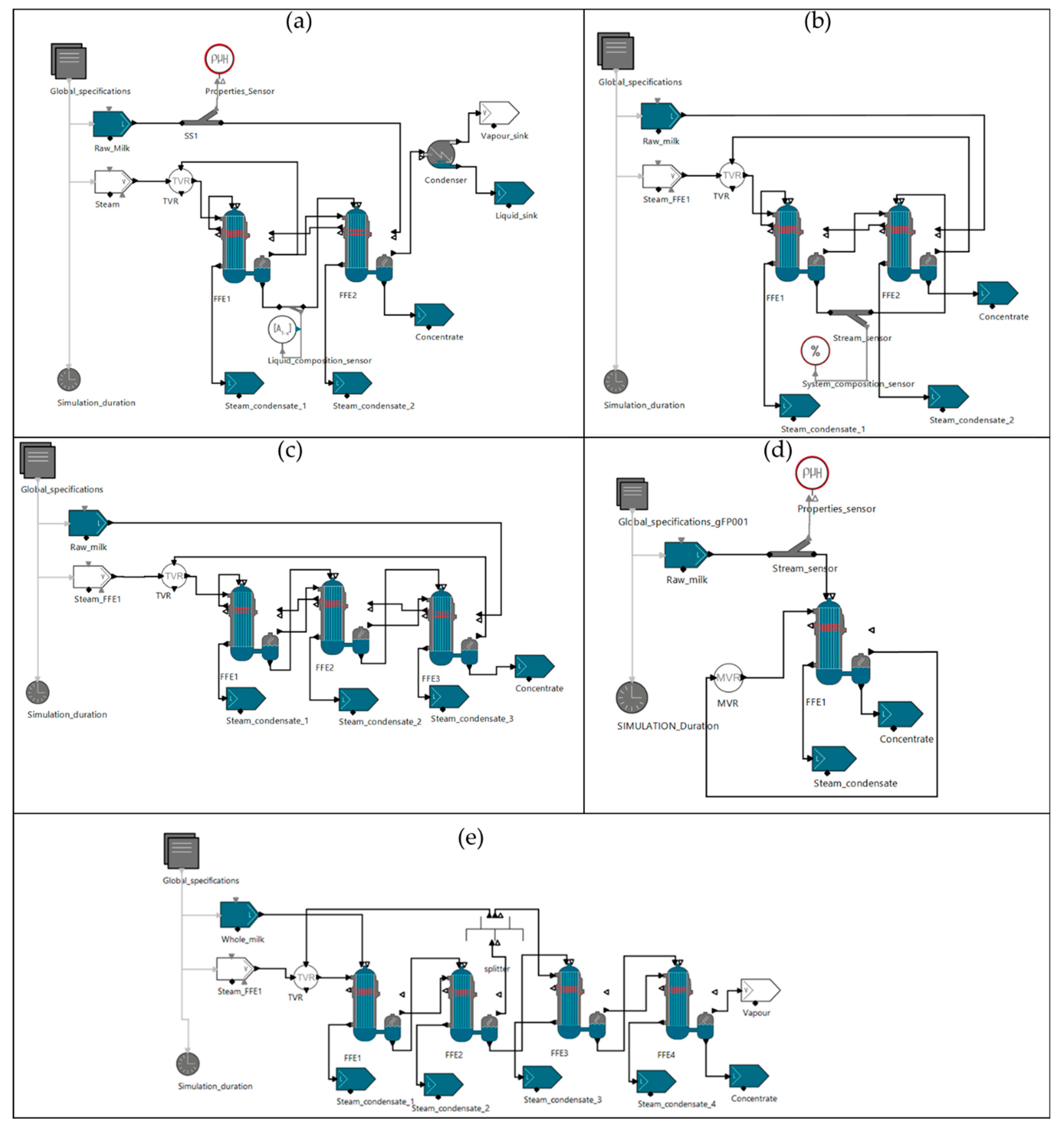
Figure 2.
Case 1 uncertainty analysis results: (a) Concentrate water mass fraction versus feed temperature and TVR discharge pressure, (b) Steam economy versus TVR suction ratio and feed temperature, (c) Steam mass flowrate versus suction ratio and TVR discharge pressure, (d) Concentrate pressure versus TVR discharge pressure and feed temperature, (e) FFE1 product dry mass fraction versus TVR suction ratio and discharge pressure.
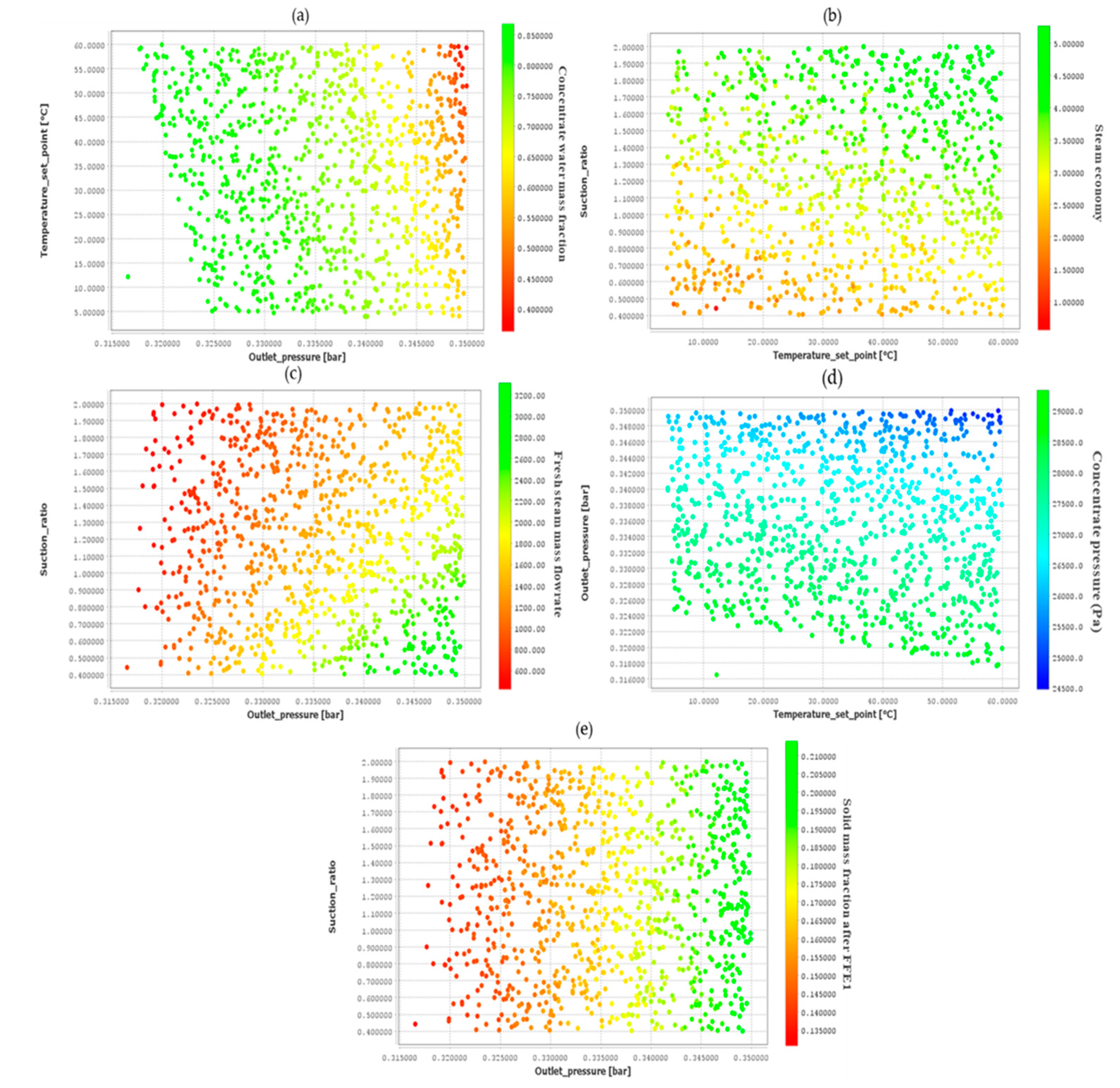
Figure 3.
Case 2 uncertainty analysis results: (a) Steam economy versus TVR suction ratio and feed temperature, (b) FFE1 product dry mass fraction versus feed temperature and discharge pressure, (c) Steam annual cost versus feed temperature and TVR discharge pressure.
Figure 3.
Case 2 uncertainty analysis results: (a) Steam economy versus TVR suction ratio and feed temperature, (b) FFE1 product dry mass fraction versus feed temperature and discharge pressure, (c) Steam annual cost versus feed temperature and TVR discharge pressure.
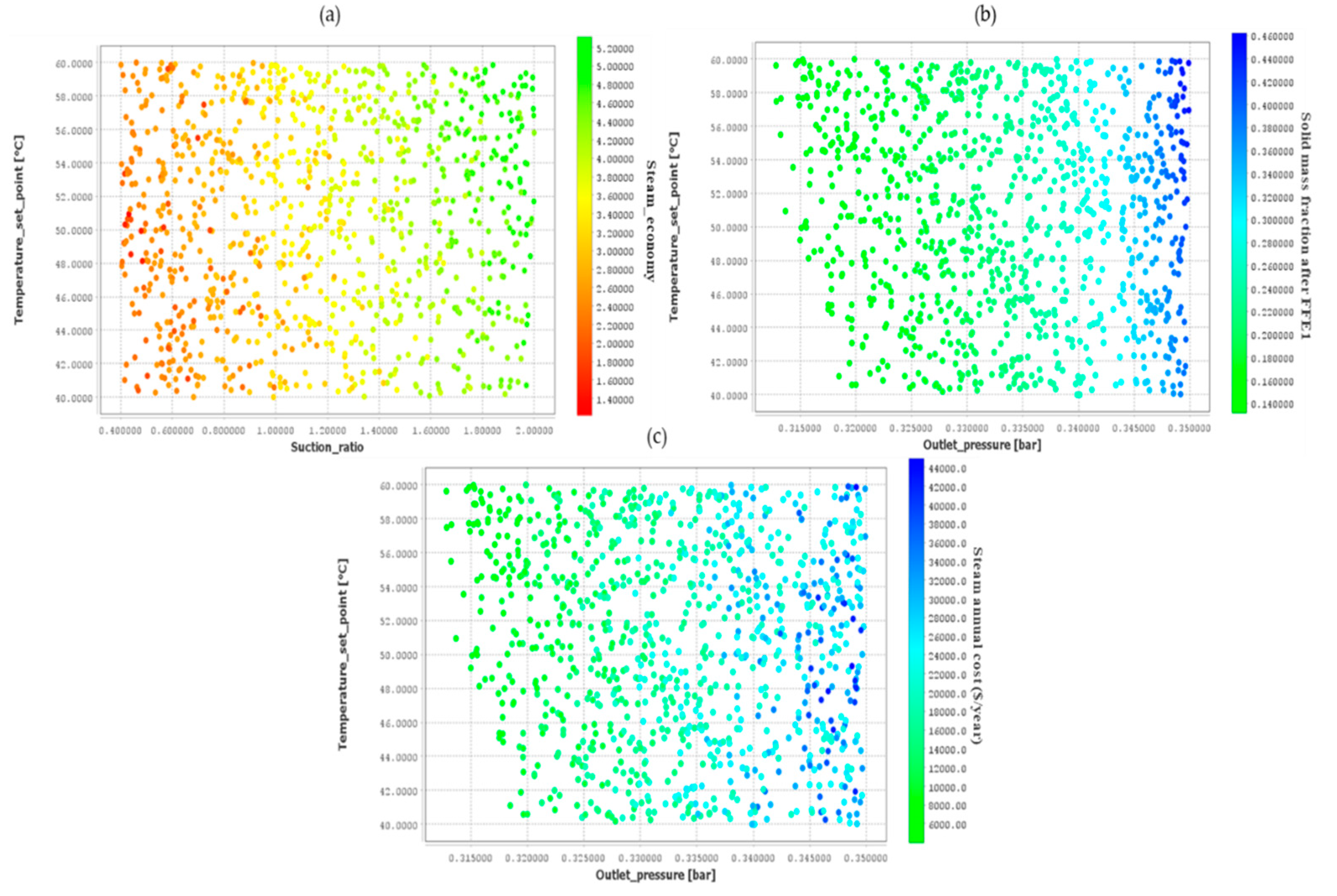
Figure 4.
Case 3 uncertainty analysis results: (a) Steam economy versus feed temperature and suction ratio, (b) Dry mass fraction of product after FFE1 versus suction ratio and TVR discharge pressure, (c) Dry mass fraction of product after FFE2 versus suction ratio and TVR discharge pressure, (d) Water mass fraction of concentrate versus TVR suction ratio and TVR discharge pressure, (e) Steam annual cost versus TVR suction ratio and TVR discharge pressure.
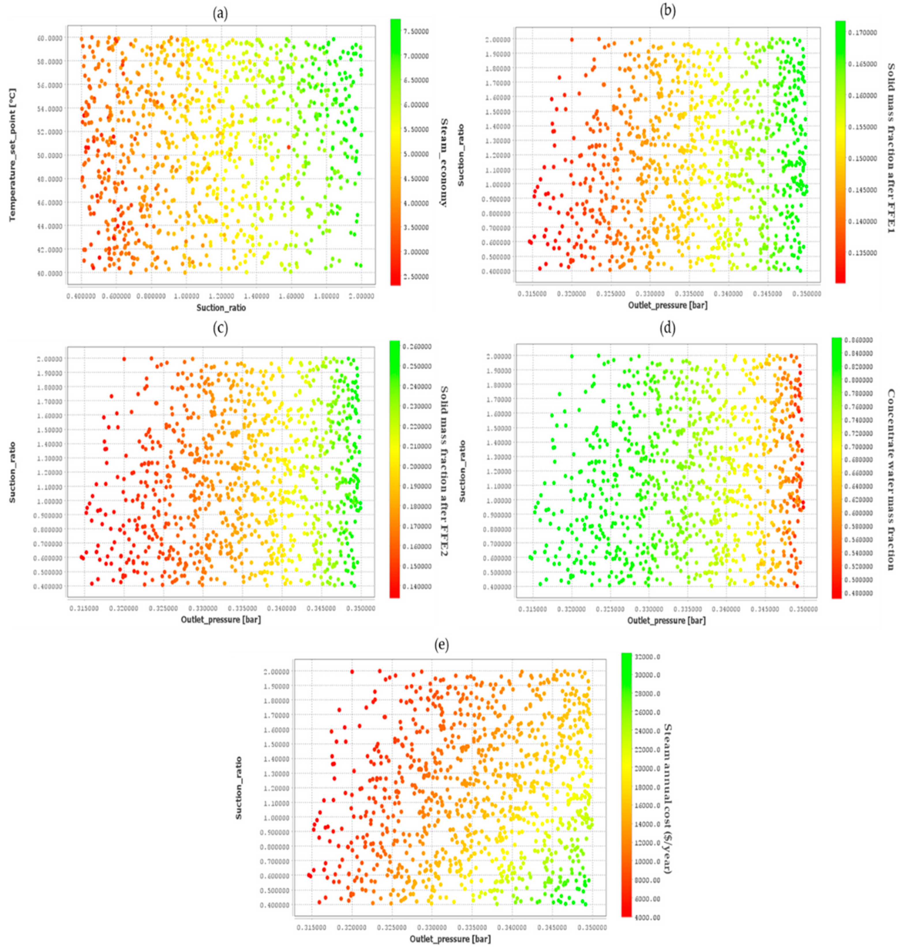
Figure 5.
Case 4 uncertainty analysis results: (a) Water mass fraction of concentrate versus feed temperature and MVR compression ratio, (b) Steam annual cost versus feed temperature and compression ratio, (c) Concentrate pressure versus MVR compression ratio and feed temperature.
Figure 5.
Case 4 uncertainty analysis results: (a) Water mass fraction of concentrate versus feed temperature and MVR compression ratio, (b) Steam annual cost versus feed temperature and compression ratio, (c) Concentrate pressure versus MVR compression ratio and feed temperature.
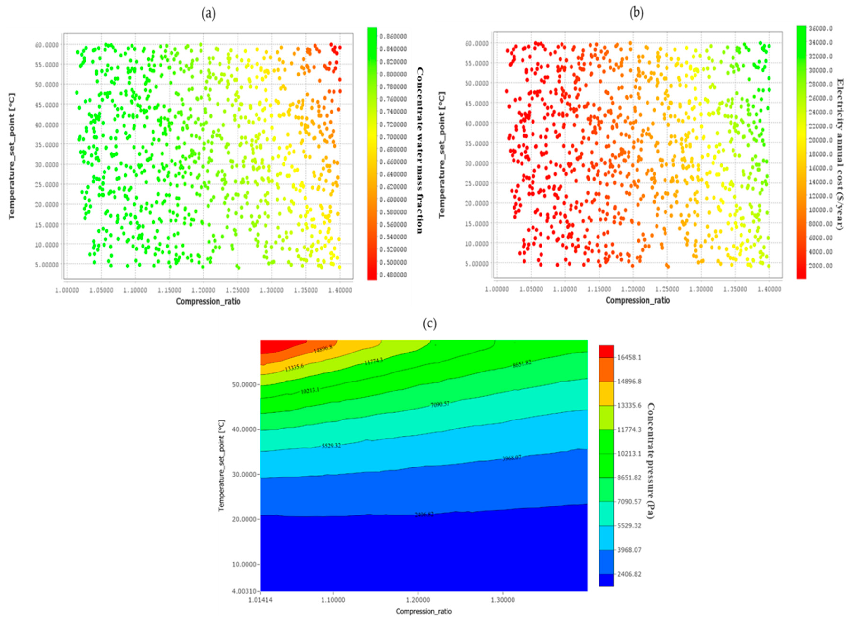
Figure 6.
Case 5 uncertainty analysis results: (a) Water mass fraction of concentrate versus feed temperature and split fraction, (b) Yield versus feed temperature and split fraction, (c) Steam annual cost versus TVR suction ratio and split fraction.
Figure 6.
Case 5 uncertainty analysis results: (a) Water mass fraction of concentrate versus feed temperature and split fraction, (b) Yield versus feed temperature and split fraction, (c) Steam annual cost versus TVR suction ratio and split fraction.
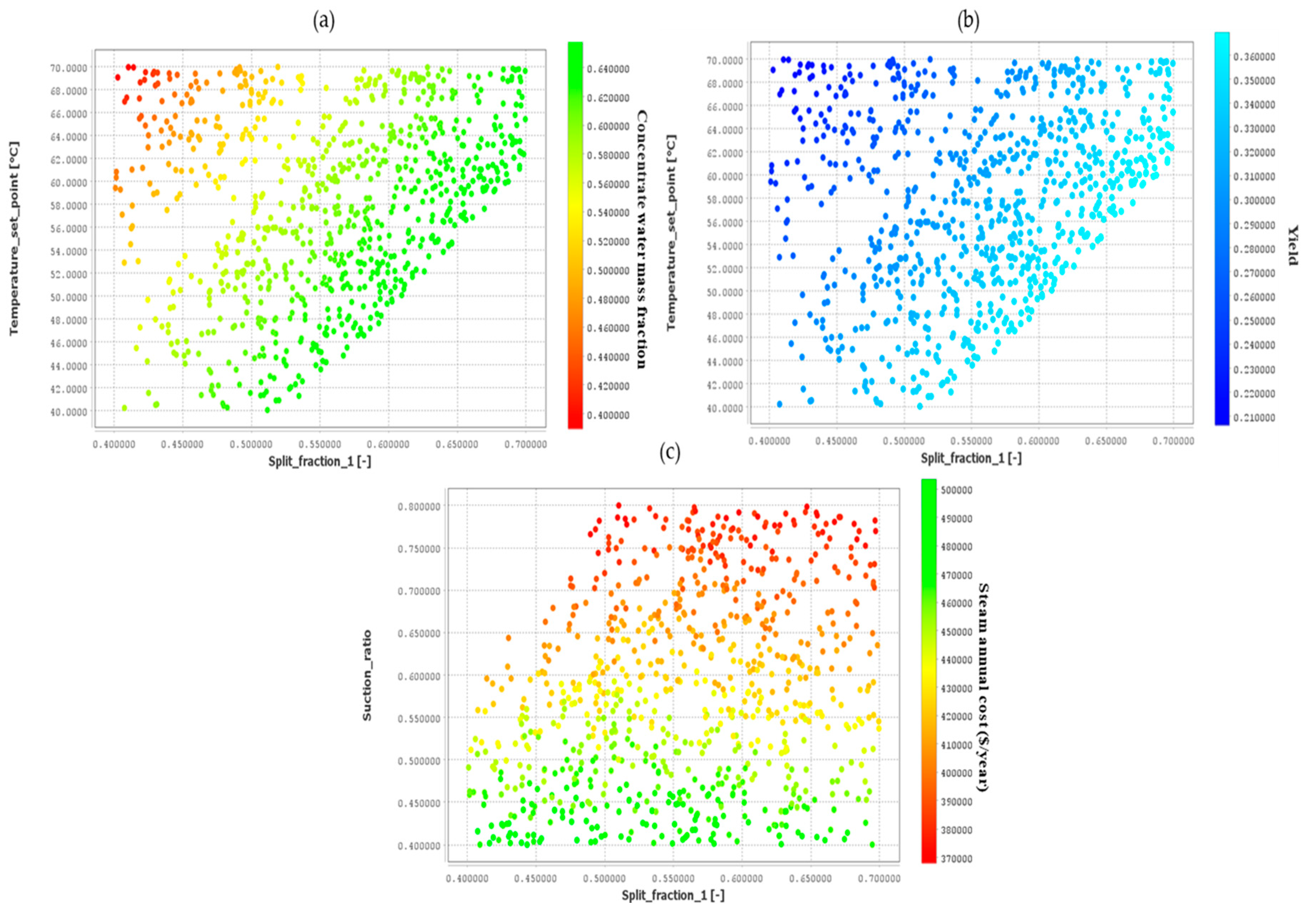

Table 1.
Whole milk composition.
| Whole milk components [24] | Weight (%) [24] |
Whole milk components [5] | Weight (%) [5] |
|---|---|---|---|
| Water | Water | ||
| Carbohydrates | Fat | ||
| Proteins | Protein | ||
| Fat | Lactose | ||
| Ash | NaCl | ||
| KCl |
Table 2.
Equations of properties calculation.
| Property | Equation [23] | |
|---|---|---|
| Specific heat capacity | ||
| Thermal conductivity | ||
| Density |
* Where is the component mass fraction.
Table 3.
Properties of whole milk before evaporation at 4°C, 101 kPa.
| Property | Value [23] | Value [5] | Simulated data |
|---|---|---|---|
| Density | |||
Table 4.
Steam prices examined in GSA.
| Cost ($/tn) | -40% | -30% | -20% | -10% | 0% | +10% | +20% | +30% |
|---|---|---|---|---|---|---|---|---|
| Biomass- based steam | 12.222 | 14.259 | 16.296 | 18.333 | 20.37 | 22.407 | 24.444 | 26.481 |
| Solar-based steam | 19.5 | 22.75 | 26 | 29.25 | 32.5 | 35.75 | 39 | 42.25 |
| Biogas-based steam | 16.452 | 19.194 | 21.936 | 24.678 | 27.42 | 30.162 | 32.904 | 35.646 |
| NG-based steam | 10.086 | 11.767 | 13.448 | 15.129 | 16.81 | 18.491 | 20.172 | 21.853 |
Table 5.
Minimum & maximum annual cost values of evaporation process depending on steam source.
| -40% | -30% | -20% | -10% | 0% | +10% | +20% | +30% | |
|---|---|---|---|---|---|---|---|---|
| Minimum Annual Cost ($) | ||||||||
| Biomass- based steam | 82,477 | 96,221 | 109,969 | 123,715 | 137,461 | 151,207 | 164,953 | 178,699 |
| Solar-based steam | 131,590 | 153,522 | 175,453 | 197,385 | 219,317 | 241,248 | 263,180 | 285,112 |
| Biogas-based steam | 111,025 | 129,525 | 148,028 | 166,532 | 185,036 | 203,539 | 222,043 | 240,546 |
| NG-based steam | 68,062 | 79,406 | 90,750 | 102,094 | 113,438 | 124,781 | 136,125 | 147,469 |
| Maximum Annual Cost ($) | ||||||||
| Biomass- based steam | 278,931 | 325,419 | 371,908 | 418,396 | 464,885 | 511,373 | 557,862 | 604,350 |
| Solar-based steam | 445,029 | 519,201 | 593,373 | 667,544 | 741,716 | 815,887 | 890,059 | 964,231 |
| Biogas-based steam | 375,468 | 438,046 | 500,624 | 563,202 | 625,780 | 688,358 | 750,936 | 813,514 |
| NG-based steam | 230,183 | 268,547 | 306,911 | 345,275 | 383,638 | 422,002 | 460,366 | 498,730 |
Table 6.
Minimum and maximum values of outlet dry mass fraction of each effect.
| Variable | Minimum | Maximum |
|---|---|---|
| FFE1 Outlet dry mass fraction (kg/kg) | 0.162 | 0.169 |
| FFE2 Outlet dry mass fraction (kg/kg) | 0.225 | 0.254 |
| FFE3 Outlet dry mass fraction (kg/kg) | 0.278 | 0.359 |
| FFE4 Outlet dry mass fraction (kg/kg) | 0.341 | 0.610 |
Table 7.
Optimization scenarios examined – Cases 1-4.
| Scenario | Objective function | Product quality specifications |
|---|---|---|
| 1 | Minimization of annual steam cost ($/year) | Product dry mass fraction = 0.5 |
| 2 | Minimization of annual steam cost ($/year) | Product dry mass fraction = 0.35 |
| 3 | Minimization of annual steam cost ($/year) | Product dry mass fraction = 0.30 |
| 4 | Maximization of yield | Product dry mass fraction = 0.5 |
| 5 | Minimization of total cost | Product dry mass fraction = 0.5 |
| 6 | Maximization of yield | 0.3 <Product dry mass fraction < 0.5 |
Table 8.
Operating constraints for Case 1.
| Constraints | Explanation |
|---|---|
| The final water content must be equal to 0.5 in Scenarios 1,4 and 5, 0.65 in Scenario 2 and 0.7 in Scenario 3. | |
| FFE1 temperature should be under 70°C to mitigate the negative effects of heat on heat-sensitive milk components and prevent the degradation of essential nutrients. | |
| The temperature of each evaporator effect must be at least 2°C lower than the previous one to ensure proper vacuum. | |
| Only for Scenario 6, the final water content varies between 0.5 and 0.7 |
Table 9.
Optimal values of performance indices, time-invariant optimization variables, and final process variables at each Scenario – Case 1.
Table 9.
Optimal values of performance indices, time-invariant optimization variables, and final process variables at each Scenario – Case 1.
| Scenario | 1 | 2 | 3 | 4 | 5 | 6 | Base Case |
|---|---|---|---|---|---|---|---|
| Steam annual cost ($/year) | 232,118 | 199,609 | 181,563 | 319,363 | 228,307 | 261,481 | 368,653 |
| Total annualized cost ($/year) | 3.90·106 | 3.86·106 | 3.85·106 | 3.98·106 | 2.33·106 | 3.92·106 | 4.03·106 |
| Yield | 0.24 | 0.36 | 0.42 | 0.252 | 0.252 | 0.42 | 0.27 |
| TVR – Discharge Pressure (bar) | 0.347 | 0.341 | 0.338 | 0.35 | 0.35 | 0.342 | 0.35 |
| TVR – Suction ratio | 2 | 2 | 2 | 1.4 | 2 | 1.4 | 1.1 |
| Feed Temperature (°C) | 60 | 60 | 60 | 31.84 | 60 | 26.74 | 20 |
| FFE1/FFE2 tube inner diameter (m) | 0.0508 | 0.0508 | 0.0508 | 0.0508 | 0.0435/0.0254 | 0.0508 | 0.0508 |
| FFE1/FFE2 tube length (m) | 16 | 16 | 16 | 16 | 17/5 | 16 | 16 |
| FFE2 Temperature (K) | 339.81 | 340.2 | 340.4 | 339.85 | 326.54 | 340.5 | 340 |
| Concentrate water content | 0.5 | 0.65 | 0.7 | 0.5 | 0.5 | 0.7 | 0.543 |
Table 10.
Optimal values of performance indices, time-invariant optimization variables, and final process variables at each Scenario – Case 2.
Table 10.
Optimal values of performance indices, time-invariant optimization variables, and final process variables at each Scenario – Case 2.
| Scenario | 1 | 2 | 3 | 4 | 5 | 6 | Base Case |
|---|---|---|---|---|---|---|---|
| Steam annual cost ($/year) | 21,159 | 18,887 | 17,184 | 30,719 | 20,663 | 25,326 | 30,740 |
| Total annualized cost ($/year) | 504,490 | 502,217 | 500,514 | 514,049 | 274,768 | 508,657 | 514,070 |
| Yield | 0.279 | 0.36 | 0.42 | 0.28 | 0.252 | 0.42 | 0.28 |
| TVR – Discharge Pressure (bar) | 0.349 | 0.345 | 0.341 | 0.35 | 0.35 | 0.342 | 0.35 |
| TVR – Suction ratio | 2 | 2 | 2 | 1.1 | 2 | 1.1 | 1.1 |
| Feed Temperature (°C) | 60 | 60 | 60 | 55.87 | 60 | 53.47 | 55 |
| FFE1/FFE2 tube inner diameter (m) | 0.0508 | 0.0508 | 0.0508 | 0.0508 | 0.0508/ | ||
| FFE1/FFE2 tube length (m) | 6 | 6 | 6 | 6 | 5.7/0.6 | 6 | 6 |
| FFE2 Temperature (K) | 340 | 340.3 | 340.5 | 340 | 293.15 | 340.5 | 340 |
| Concentrate water content | 0.5 | 0.65 | 0.7 | 0.5 | 0.5 | 0.7 | 0.55 |
Table 11.
Operating constraints for Case 3.
| Constraints | Explanation |
|---|---|
| The final water content must be equal to 0.5 in Scenarios 1,4 and 5, 0.65 in Scenario 2 and 0.7 in Scenario 3. | |
| FFE1 temperature should be under 70°C to mitigate the negative effects of heat on heat-sensitive milk components and prevent the degradation of essential nutrients. | |
| The temperature of each evaporator effect must be at least 2°C lower than the previous one to ensure proper vacuum. | |
| Only for Scenario 6, final water content can vary between 0.5 and 0.7 |
Table 12.
Optimal values of performance indices, time-invariant optimization variables, and final process variables at each Scenario – Case 3.
Table 12.
Optimal values of performance indices, time-invariant optimization variables, and final process variables at each Scenario – Case 3.
| Scenario | 1 | 2 | 3 | 4 | 5 | 6 | Base Case |
|---|---|---|---|---|---|---|---|
| Steam annual cost ($/year) | 15,078 | 12,989 | 11,300 | 22,069 | 18,900 | 19,200 | 22,088 |
| Total annualized cost ($/year) | 681,251 | 679,163 | 677,474 | 688,242 | 449,236 | 685,374 | 688,262 |
| Yield | 0.25 | 0.35 | 0.36 | 0.252 | 0.25 | 0.36 | 0.25 |
| TVR – Discharge Pressure (bar) | 0.35 | 0.342 | 0.34 | 0.35 | 0.349 | 0.344 | 0.35 |
| TVR – Suction ratio | 2 | 2 | 2 | 1.1 | 1.37 | 1.1 | 1.1 |
| Feed Temperature (°C) | 60 | 60 | 60 | 54.9 | 60 | 53.6 | 55 |
| FFE1/FFE2/FFE3 tube inner diameter (m) | 0.0508 | 0.0508 | 0.0508 | 0.0508 | 0.0508 / 0.0381/0.0381 | 0.0508 | 0.0508 |
| FFE1/FFE2/FFE3 tube length (m) | 6 | 6 | 6 | 6 | 4.25/4.12/4.13 | 6 | 6 |
| FFE2 Temperature (K) | 340.7 | 341 | 341 | 340.7 | 338.5 | 341 | 340.7 |
| FFE3 Temperature (K) | 338.3 | 338.9 | 339 | 338.4 | 334 | 339 | 338.4 |
| Concentrate water content | 0.5 | 0.65 | 0.7 | 0.5 | 0.5 | 0.7 | 0.5 |
Table 13.
Constraints and explanations - Case 4.
| Constraints | Explanation |
|---|---|
| The final water content must be equal to 0.5 in Scenarios 1,4 and 5, 0.65 in Scenario 2 and 0.7 in Scenario 3. | |
| FFE1 temperature should be under 70°C to mitigate the negative effects of heat on heat-sensitive milk components and prevent the degradation of essential nutrients. | |
| Only for Scenario 6, final water content can vary between 0.5 and 0.7 |
Table 14.
Optimal values of performance indices, time-invariant optimization variables, and final process variables at each Scenario – Case 4.
Table 14.
Optimal values of performance indices, time-invariant optimization variables, and final process variables at each Scenario – Case 4.
| Scenario | 1 | 2 | 3 | 4 | 5 | 6 | Base Case |
|---|---|---|---|---|---|---|---|
| Electricity annual cost ($/year) | 34,319 | 23,815 | 19,299 | 35,950 | 39,522 | 20,466 | 34,582 |
| Total annualized cost ($/year) | 275,985 | 265,480 | 260,964 | 277,616 | 251,240 | 262,131 | 276,248 |
| Yield | 0.252 | 0.36 | 0.42 | 0.252 | 0.252 | 0.42 | 0.26 |
| MVR – Adiabatic efficiency | 1 | 1 | 1 | 0.98 | 1 | 1 | 1 |
| MVR – Compression ratio | 1.38 | 1.3 | 1.26 | 1.4 | 1.45 | 1.29 | 1.4 |
| Feed Temperature (°C) | 60 | 60 | 60 | 50.35 | 60 | 44.17 | 50 |
| FFE1 tube inner diameter (m) | 0.0508 | 0.0508 | 0.0508 | 0.0508 | 0.0508 | 0.0508 | 0.0508 |
| FFE1 tube length (m) | 6 | 6 | 6 | 6 | 5.7 | 6 | 6 |
| FFE1 Temperature (K) | 319.2 | 321 | 322.1 | 312.5 | 318.6 | 310.3 | 312.3 |
| Concentrate water content | 0.5 | 0.65 | 0.7 | 0.5 | 0.5 | 0.7 | 0.514 |
Disclaimer/Publisher’s Note: The statements, opinions and data contained in all publications are solely those of the individual author(s) and contributor(s) and not of MDPI and/or the editor(s). MDPI and/or the editor(s) disclaim responsibility for any injury to people or property resulting from any ideas, methods, instructions or products referred to in the content. |
© 2023 by the authors. Licensee MDPI, Basel, Switzerland. This article is an open access article distributed under the terms and conditions of the Creative Commons Attribution (CC BY) license (http://creativecommons.org/licenses/by/4.0/).
Copyright: This open access article is published under a Creative Commons CC BY 4.0 license, which permit the free download, distribution, and reuse, provided that the author and preprint are cited in any reuse.


