
Submitted:
30 October 2023
Posted:
03 November 2023
You are already at the latest version
Abstract
The rise of digital technology and artificial intelligence has led to a significant change in the way financial services are delivered. One such development is the emergence of robo-advising, which is an automated investment advisory service that utilizes algorithms to provide investment advice and portfolio management to investors. Robo-Advisors collect information about their clients’ preferences, financial situation and future goals through questionnaires, then recommend ETF based portfolios supposed to fit investor’s risk profile. However, questionnaires seem to be vague, and robos do not reveal the methods used for investor profiling or asset allocation. This study aims at contributing by proposing an investor profiling method, based only on the level of relative risk aversion (RRA) of investors. We show how to determine RRA optimal portfolios and compare the performance of our portfolios with portfolios proposed by the Riskalyze platform.
Keywords:
robo-advisor
; mean variance theory
; expected utility theory
; sharpe ratio
1. Introduction
Banking is necessary, banks are not is a famous quote from Microsoft founder Bill Gates, which characterizes the wide debate of the increasing digitalization of banking [1].
Nowadays, the technological world has been growing at a very fast rate, which means there has to be a quick adaptation and companies feel the need to reinvent themselves. Technological innovations also reached the asset management service industry with the so-called Robo-Advisors.
Robo-advising, also known as automated investment management or digital wealth management, has become increasingly popular in the investment industry over the past few years. The evolution of robo-advising can be traced back to the early 2000s, when the first online investment platforms were launched. However, it was not until the mid-2010s that robo-advising really began to take off.
The first wave of robo-advisors were standalone digital investment platforms, such as Betterment and Wealthfront, that offered algorithm-driven portfolio management to retail investors. These platforms typically used low-cost ETFs to build diversified portfolios, and charged lower fees than traditional human financial advisors.
As robo-advising gained popularity, traditional financial institutions began to take notice and started offering their own digital investment services. This led to the second wave of robo-advisors, which included offerings from established firms such as Vanguard, Charles Schwab, and Fidelity.
In addition to standalone platforms and offerings from traditional firms, some robo-advisors have also partnered with financial advisors to offer a hybrid model of digital and human advice. This allows investors to access the benefits of technology-driven portfolio management, while still having access to human guidance when they need it.
One can say the evolution of robo-advising has democratized access to investment management, making it easier and more affordable for retail investors to build diversified portfolios. For an overview of the pre-pandemic evolution of robo advising, highlighting the path of regulation in the area, we refer to [2].
The truth is that with the outbreak of COVID-19 pandemic bank clients showed higher readiness to adopt an algorithm advice [3], which helped accelerating even further the digitalisation of the financial system. Robo-advising is becoming increasingly popular among investors due to its lower cost, convenience, and ease of use.
Despite its evolution and popularity there has been a very limited number of studies comparing the performance of portfolios proposed by robos, to traditional mutual funds. One exception is [4], but the main reason for the absence of studies is that robos do not disclose their portfolios, in addition they claim to taylor a portfolio for each investor, making it impossible to compare with traditional mutual funds.
Another “grey” area of robo-advising is the evaluation of each investor risk profile. The assessment of risk preferences tends to be rather vague, with very significant differences between robos [5].
In this study we look at actual portfolios proposed by Riskalyze – one of the most well-known US robo-advisors – for three made-up profiles: conservative, moderate and aggressive investors. The Riskalyze portfolios are the ones in [6]. We compare in-sample and out-of-sample performance of those real-life portfolios with mean-variance theory (MVT) optional portfolios, for investors with different levels of relative risk aversion (RRA). A method of investor classification that is simple, while allowing discrimination of investors beyond the traditional 3 broad classes.
The remaining of the paper is organized as follows. Section 2 presents an overview of the literature on robo-advising. In Section 3 we detail the methodology and data used. Section 4 presents and discussed the results. Finally, Section 5 concludes, presents the limitations of the analysis and suggests further research.
2. Literature Review
This review explores the, still incipient, academic literature on robo-advising, focusing on its growth, benefits, challenges, and future prospects.
Robo-advising has seen a rapid growth in recent years due to the rise of digital technology and increased interest in passive investing. According to some reports, since 2013 this technological revolution has been increasing by 24% on average each year – see for instance the annual Executive Summaries World Robotics of the International Federation of Robotics (IFR) –, and it is expected that they will replace 47% of the current jobs in the next 20 years [7]. A report by Deloitte estimated that robo-advisors managed $2.2 trillion and $3.7 trillion in assets under management (AuM) in 2020 and projected that this would increase to $16 trillion by 2025, roughly three times the amount of assets managed by BlackRock, the word’s biggest asset manager to date [8]. COVID also helped to boost this rapid adaptation to technology and digital platforms [3,9].
Robo-advising offers several benefits to investors, including lower fees, portfolio diversification, and personalized investment advice. As robo-advisors offered lower fees than traditional advisors, it could potentially lead to higher returns for investors over time [4,10]. According to [11] robo-advisors provided better portfolio diversification than traditional advisors, resulting in a lower risk for investors. Additionally, robo-advisors can provide personalised investment advice and mitigate some behavioural biases [12,13].
Despite the benefits of robo-advising, there are also several challenges that must be addressed. One of the primary concerns is the lack of human interaction, which may make it difficult for investors to understand the investment advice provided by robo-advisors, [14]. Still nowadays, specially when it comes to trust, investors prefer human expert financial advisors [15,16]. Another challenge is the potential for algorithmic bias, which may lead to suboptimal investment decisions. For instance, robo-advisors are less likely to recommend socially responsible investments, which may be due to the lack of data on these investments [17]. There is also a tendency to propose products (ETFs) managed by the same entity, and not to consider competitors. Finally, robo-advising has raised regulatory questions related to investor protection, compliance, and oversight. [18]. Regulatory bodies have had to adapt to the evolving landscape to ensure investor safety and adherence to existing financial regulations. Nonetheless, it is unclear how exactly robo-advisors do investors’ risk profiling and how that actually impacts the proposed portfolios. [19] show robos are able to identify differences in profiles, but when it comes to portfolio allocations, the variability across robos, for the same type of investor, is hard to justify.
The future prospects of robo-advising are promising, as the technology continues to improve and investors become more comfortable with automated investment advice. One potential area of growth is the integration of robo-advising with traditional advisory services, which may provide investors with the “best of both worlds”[1]. Additionally, the use of artificial intelligence (AI) and machine learning may enable robo-advisors to provide more personalized investment advice based on an investor’s unique circumstances. See [20,21,22,23] for proposals on concrete ways to include AI into robo advising. Beyond traditional investment management, robo-advisors are expanding into other financial services. This includes offering services like financial planning, retirement planning, and even banking services. The goal is to provide a comprehensive suite of financial products and advice through a single platform. Improvements in data analytics, artificial intelligence, and automation are expected to make these platforms more efficient and capable of providing more sophisticated investment advice. Moreover, advancements in cybersecurity are crucial to maintain the trust of investors.
In this study we propose a method to classify investors, based upon mean-variance theory [24] and expected-utility theory [25] and the simple measure of relative risk aversion (RRA). We then capture the in-sample and out-of-sample performance of real portfolios proposed by Riskalyze comparing them to RRA optimal portfolios.
Although we consider directly various levels of RRA, there is some recent literature on risk profiling that is worth mentioning. [26] proposes a method of measuring investor’s risk apetite based upon a ratio between risk-neutral and subjective probabilities. [27] presents an improved measurement of subjective risk tolerance and discusses its link to relative risk aversion. [28] suggest robo-advisors could use portfolio choices to learn investor’s risk preferences. [29] propose a sophisticated model to evaluate risk profile.
3. Methodology & Data
The aim of this study is to use mean-variance theory (MVT) and expected-utility theory (EUT) to identify optional portfolios, for investors with different levels of relative risk aversion (RRA). We then compare in- and out-of-sample performances of these theoretically optimal portfolios, with those of Riskalyze actual portfolio proposals for conservative, moderate and aggressive investors.
3.1. Mean-Variance Portfolios
Given a set of risky assets, MVT allows to find all efficient portfolios. That is, all portfolios with biggest expected return for a given level of risk, or with the least risk for a given level of expected return.
MVT is still the “standard” portfolio building method, widely used, not only by academics, but also by practitioners. Given a set of n risky assets with individual expected returns , for , the expected return of any portfolio p is given by,
where, shows the weight of each individual asset in a portfolio, and we have
The risk of a portfolio, as evaluated by the variance is given by,
where denotes the covariance between the returns of asset i and j.
In vector notation we can use
and get
In this study we focus on MVT efficient portfolios: the tangent (T) portfolio, the minimum variance (MV) portfolio, as well as optimal portfolios for various levels of relative risk aversion (RRA). Since we are considering short-selling is not allowed (all robo portfolios seem to impose such a restriction), we must rely on numerical solutions to the following optimization problems.
The tangent (T) portfolio is the one with the highest Sharpe ratio, so it solves
where denotes a vector of ones and the inequality restrictions are the ones imposing no shortselling.
The minimum variance (MV) portfolio, solves
We also consider optimal MVT portfolios for investors with different levels of relative risk aversion (RRA). So we take the investor’s perspective, and analyze preferences. In modelling choice under uncertainty we consider EUT of Von Neumann and Morgenstern [25] to model economic agents’ decisions. In this context the so-called risk tolerance function is nothing but the expected utility of terminal wealth.
Following [32], we rely on the common second-order Taylor approximation for the risk tolerance function, which is valid for all utility functions
where denotes the relative risk aversion of the investor evaluated at initial wealth.
One of the advantages of Equation (3) is that it only depends on the initial level of of investors. So by varying we are able to capture very different profiles. For values between -1 and 6, we capture various investor profiles, from the risk lover (), to the risk neutral () and all sorts of risk aversion with different degrees RRA = {1,2,3,4,5,6}. Empirical evidence seems to point to as realistic levels of . Here we go beyond those values of purpose to include all types of investors, from risk lover to extreme risk aversion.
The optimal portfolio for a particular investor (with a particular level of ) solves the following problem,
3.2. Robo Portfolios
We have information only on three portfolios from Riskalyze, one for each broad classification of investors: conservative, moderate and aggressive. The data for these portfolios comes from [6] that on the 31st March 2017, using real investments at the Riskalyze platform, obtained three portfolio compositions answering as conservative, moderate and aggressive investors willing to invest for 5-years.
The aggressive investors are the ones that are enthusiastic in taking large amounts of risk and do not settle back when observe downward movements in their portfolios. They usually go for the risky asset classes, and when the market is performing well, they invest in the assets that present higher returns. Moderate investors are willing to take some risk, and they can handle until a certain percentage a downward in their portfolio before taking their money. They usually invest part of their money in riskier assets and the other part in safer assets. Conservative investors are the ones that are hardly able to take any risk, so they always go for the safest assets, the ones that offer them capital protection, since they do not want to suffer losses. The risk tolerance of each investor is influenced by some determining factors, such as the financial situation, asset class preference, time horizon and the purpose of the investment. Still nowadays most robos, rely on broad investor classifications such as the one they use.
3.3. Homogeneous Portfolio
In addition to the above mentioned MVT and robo portfolios, we also consider the homogeneous, H, portfolio as a naïve benchmark.
3.4. Investment Strategy and Performance Evaluation
We make a comparative analysis of the performance of all portfolios previously mentioned, where we start by estimate the amount that is allocated to each asset. For this, we consider we invest $100 in each portfolio, and see how it evolves until maturity. We consider a monthly rebalancing, in order to realign the weightings of the portfolios. We opt for the monthly rebalancing, because according to [33], the monthly rebalancing presents the best outperformances when unit transaction costs are below approximately 50 basis points, and costs associated with ETFs are low.
In addition to the evolution, we calculate the Sharpe ratio (SR) for each portfolio both in-sample and out-of-sample, since it is commonly used as a performance measurement. Besides being a classical measure of perforance, according to [34], this performance measure is also related to the “level of maximum expected utility provided by the asset”, which means when an asset present a greater performance measure, the asset provides a higher level of maximum expected utility.
The portfolio Sharpe ratio is defined as
where, is the expected return of the portfolio, is the volatility of the portfolio (as previously defined) and is the risk-free interest rate of the market.
3.5. Data
To carry out this study, we use data from
- the composition, on Mach 31 2017, of three Riskalyze portfolios for conservative, moderate and aggressive, respectively, for an investment horizon of 5 years.
- daily prices for all 15 ETFs in the Riskalyze portfolio compositions, from 1st March 2012 to 31st March 2020.
Table 1 presents the ETFs description, abbreviations and categories. We use the first 5-year period for the in-sample calculations. For out-of-sample performance we consider from 1st April 2017 to 31st March 2020. The out-of-sample period, finishes in the 31st March 2020, in order not to bias our analysis with the COVID-19 pandemic crisis effect.
In addition to the 15 ETFs provided by the platform, we also consider a risk free asset, in this case the 5-year US Treasury Bond yields (0.16%).
Figure 1 presents the evolution of the prices of each ETF. At the very end of out sample (in March 2020) we still capture some of the COVID-19 impact.
We use the first 5-years of data to estimate mean-variance inputs: Table A1-Table A2 present the vector of expected returns and the variance-covariance matrix.
Figure 2 shows the mean-variance representation of the ETFs. It considers only the in-sample data, so data before March 31 2017, and we have simply computed historical averages and standard deviations of returns using a sample size equal to the investment horizon.. This is information Riskalize had at the time they proposed their portfolios. Some of the recommended ETFs had done particularly bad in the previous 5 years.
4. Results
4.1. In-Sample Results
Not surprisingly, when we impose shortselling restrictions, the MVT portfolios end up investing in a limited number of ETFs. But so do the Riskalize portfolios with the conservative investing in 7 ETFs, the moderate in 10 ETFs and the aggressive in 8 ETFs.
Optimal portfolios according to vary from 100% invested in highest expected return ETF (for risk lovers, risk neutral and risk averse with up to RRA=0.5), to a maximimum of 6 ETFs out of a set of just 7 ETFs, for all other values.
In terms of statistics we see the tangent portfolio T does maximize Sharpe ratio, but at the cost of low volatility and expected returns. The homogeneous portfolio have an expected return around 6% with a volatility around 8%, so a Sharpe ratio around 0.7. H does better on both dimensions than the Riskalize conservative portfolio C, worse than the moderate portfolio M, and in line with the aggressive portfolio A.
However, the portfolios that are optimal according to are the ones with relatively high Sharpe ratios, for realistic levels of expected returns and volatility. All Sharpe ratios range from 1.0770 to 1.4045 increasing with the level of risk aversion. Expected returns and volatility also decrease for increasing RRAs.
Figure 3 shows the (in sample) mean-variance representation of all portfolios.
It is possible to see that the robo-portfolios, as well as the naive homogeneous portfolio, are inside the historical efficient frontier (EF), which tell us those portfolios must be selected according to criteria other than mean-variance efficiency or that the inputs used by the Robo-advisor substantially differed from the historical ones. The EF itself includes subsets of different hyperbolas, as expected in the case of no short selling and it is also evident from the portfolio compositions in Table 3 , where the set of assets is not constant for the various optimal portfolios.
Figure 3 presents the position of the optimized portfolios with those proposed by the online platform. Comparing volatility levels, we perceive that the Riskalyze conservative portfolio has much lower risk than all our risk averse portfolios, the moderate portfolio has volatility close to the optimal portfolio when we consider , and the aggressive portfolio seems to be close to an . Since real life levels of risk aversion are less than 3, we could say the robo is ultra-convervative, even with the most aggressive portfolio.
Table 3 and Figure 3, demonstrates that in-sample optimized portfolios are more efficient. Thus, we can say that if investors aspire to efficient portfolio, optimization seems to do better. So with the data available on the market, and purely looking in-sample, the Riskalize proposed portfolios appear to be inefficient, or else the robo is are not using MVT, at least with our inputs.
In-sample comparison of portfolios is not “fair”. The true challenge is out-of-sample performance of portfolios.
4.2. Out-of-Sample
We aim to observe the actual/forward performance of portfolios proposed based only on information up to March 31 2017. As previously mentioned the investment horizon of such portfolios is 5 years, thus, until the end of March 2022. Unfortunately, our out-of-sample finishes in March 2020 because of the COVID-19 pandemic, so this out-of-sample analysis relies only on the first 3 years of investment. Still, we find our out-of-sample results to be sound.
We consider a notional investment of $100 in each portfolio, and from there see how it evolves. We assume monthly rebalancing, in order to realign the weightings of the portfolio. Figure 4, we can see how the portfolios created by us evolved from 31st March 2017 to 31st March 2020.
Only by looking in terms of evolution we see that the portfolios do considerably better than the other portfolios. The most aggressive () performing better, with the first strategy in terms of final value being that of risk lovers and risk neutral. For levels of risk aversion between 3 and 6 the performance gets close to that of the aggressive portfolio of Riskalize. The moderate portfolio of riskalize perform below all portfolios, but still higher than the worst three: the , T and the conservative Riskalize portfolio.
Table 4 presents annual values of the $ 100 investment on the 3 year out-of-sample period. The most relevant results are, however, those in Table 5 where the portfolios show up ranked – higher to lower – by Sharpe ratios. These ratios cover the investment over the entire 3 years of out-of-sample data. Once again we see the portfolios performing reasonably well. We also note that Sharpe ratios decrease for increase levels of risk aversion, as one should expect. On the other hand, the Riskalize portfolios Sharpe ratios go against the economical intuition with the conservative portfolio presenting a higher value, than the moderate portfolio and the aggressive.
5. Conclusions
The aim of this study is to propose a way for Robo-Advisors to incorporate, in portfolio building, the risk profiles of their investors. Using analytical methodologies rooted in mean-variance theory and expected utility theory, we propose the construction of relative risk aversion () optimal portfolios.
We perform a comparative analysis between 3 portfolios generated by Riskalize and those constructed by us. This comparison allowed us to conclude their methodology does not “align” with ours.
In terms of performance, our results reveal that during the in-sample period, optimizing portfolios for varying levels of RRA is more favourable than choosing portfolios provided by the Riskalyze platform. This preference is substantiated by our portfolios exhibiting a superior Sharpe Ratio, indicating enhanced portfolio performance. We also noted that the level of volatilities presented by Riskalize portfolios seem to be too low, for realistic levels of risk aversion, which usually means .
Transitioning to the out-of-sample period, we confirm the good performance of optimal portfolios. Riskalyze portfolios show Sharpe ratios from 0.18-0.33 with the surprising result that it is the conservative portfolio presenting the highest value and the aggressive presenting the lower, while portfolios with present Sharpe ratios from 0.52-0.58.
This analysis is, of course, not free of limitations. In particular we use data only on 3 portfolios proposed by Riskalize at a particular moment in time. Although interesting, one should be careful to extrapolate these results to all Riskalize portfolios and even more so to extrapolate to other robo-advisors. It would be interesting to look more systematically into real life robo portfolios, but as mentioned this is data that is simply not available. From the data we use we are able to conclude Riskalize portfolios do not seem to be mean-variance efficient (at least if we use historical MVT inputs). In addition, as portfolios for seems to “beat” in and out-of-sample those of Riskalize.
We hope this study contributes to a better understanding robo-advisors. Above all, we hope robos will start using more accurate methods of investor profiling.
Author Contributions
Conceptualization, RMG; methodology, RMG ; software, MO.; validation, RMG and MO.; formal analysis, RMG; investigation, MO; resources, RMG and MO; data curation, MO; writing—original draft preparation, MO.; writing—review and editing, RMG; visualization, RMG; supervision, RMG.; project administration, RMG; funding acquisition, RMG. All authors have read and agreed to the published version of the manuscript.
Funding
This research was partially supported by the Project CEMAPRE/REM - UIDB/05069/2020 financed by FCT/MCTES (Portuguese Science Foundation), through national funds.
Appendix A

Table A1.
In-sample expected returns and volatilities for all ETFs.
| INDEX | ||
| BND | 1.95% | 3.22% |
| SHY | 0.48% | 0.78% |
| SPY | 13.40% | 12.63% |
| EFA | 6.53% | 15.55% |
| HYG | 4.91% | 6.62% |
| FLOT | 0.98% | 0.97% |
| VNQ | 11.04% | 14.77% |
| QQQ | 16.27% | 14.96% |
| DBC | -12.05% | 14.70% |
| DBL | 8.31% | 13.81% |
| EFR | 7.16% | 10.38% |
| XLU | 12.21% | 13.88% |
| EEM | 1.39% | 19.20% |
| FPX | 16.00% | 15.51% |
| FXI | 4.51% | 23.22% |
Table A2.
In-sample variance-covariance matrix for all ETFs.
| BND | SHY | SPY | EFA | HYG | FLOT | VNQ | QQQ | DBC | DBL | EFR | XLU | EEM | FPX | FXI | |
| BND | 0.00104 | 0.00018 | -0.0009 | -0.00085 | 0.00006 | -0.00001 | 0.00083 | -0.00094 | -0.00042 | 0.00094 | -0.00007 | 0.00117 | -0.00032 | -0.001 | -0.00097 |
| SHY | 0.00018 | 0.00006 | -0.00023 | -0.00018 | -0.00003 | 0 | 0.00012 | -0.00025 | -0.00005 | 0.00011 | -0.00006 | 0.00023 | -0.00011 | -0.00026 | -0.00026 |
| SPY | -0.0009 | -0.00023 | 0.01595 | 0.01677 | 0.00577 | 0.00009 | 0.01189 | 0.01735 | 0.00726 | 0.00169 | 0.00352 | 0.00831 | 0.01874 | 0.01729 | 0.01897 |
| EFA | -0.00085 | -0.00018 | 0.01677 | 0.02419 | 0.00688 | 0.00013 | 0.01278 | 0.0178 | 0.0101 | 0.00203 | 0.00416 | 0.00869 | 0.0248 | 0.01814 | 0.0253 |
| HYG | 0.00006 | -0.00003 | 0.00577 | 0.00688 | 0.00439 | 0.00003 | 0.00508 | 0.00605 | 0.00407 | 0.00156 | 0.00205 | 0.00331 | 0.00834 | 0.00644 | 0.00783 |
| FLOT | -0.00001 | 0 | 0.00009 | 0.00013 | 0.00003 | 0.00009 | 0.00008 | 0.00007 | 0.0001 | 0.00002 | 0.00006 | 0.00005 | 0.00018 | 0.00008 | 0.0002 |
| VNQ | 0.00083 | 0.00012 | 0.01189 | 0.01278 | 0.00508 | 0.00008 | 0.02181 | 0.01195 | 0.00404 | 0.00442 | 0.00254 | 0.01284 | 0.01557 | 0.01258 | 0.01395 |
| QQQ | -0.00094 | -0.00025 | 0.01735 | 0.0178 | 0.00605 | 0.00007 | 0.01195 | 0.02238 | 0.00653 | 0.00208 | 0.00384 | 0.00742 | 0.02005 | 0.02013 | 0.02062 |
| DBC | -0.00042 | -0.00005 | 0.00726 | 0.0101 | 0.00407 | 0.0001 | 0.00404 | 0.00653 | 0.02159 | 0.00091 | 0.00234 | 0.00286 | 0.01352 | 0.00788 | 0.01202 |
| DBL | 0.00094 | 0.00011 | 0.00169 | 0.00203 | 0.00156 | 0.00002 | 0.00442 | 0.00208 | 0.00091 | 0.01908 | 0.00231 | 0.00333 | 0.00327 | 0.00197 | 0.00238 |
| EFR | -0.00007 | -0.00006 | 0.00352 | 0.00416 | 0.00205 | 0.00006 | 0.00254 | 0.00384 | 0.00234 | 0.00231 | 0.01077 | 0.00139 | 0.00453 | 0.00431 | 0.00462 |
| XLU | 0.00117 | 0.00023 | 0.00831 | 0.00869 | 0.00331 | 0.00005 | 0.01284 | 0.00742 | 0.00286 | 0.00333 | 0.00139 | 0.01927 | 0.01108 | 0.00727 | 0.00909 |
| EEM | -0.00032 | -0.00011 | 0.01874 | 0.0248 | 0.00834 | 0.00018 | 0.01557 | 0.02005 | 0.01352 | 0.00327 | 0.00453 | 0.01108 | 0.03685 | 0.0201 | 0.03779 |
| FPX | -0.001 | -0.00026 | -0.00026 | 0.01814 | 0.00644 | 0.00008 | 0.01258 | 0.02013 | 0.00788 | 0.00197 | 0.00431 | 0.00727 | 0.0201 | 0.02406 | 0.02054 |
| FXI | -0.00097 | -0.00026 | 0.01897 | 0.0253 | 0.00783 | 0.0002 | 0.01395 | 0.02062 | 0.01202 | 0.00238 | 0.00462 | 0.00909 | 0.03779 | 0.02054 | 0.05392 |
References
- Jung, D.; Dorner, V.; Glaser, F.; Morana, S. Robo-advisory: digitalization and automation of financial advisory. Business & Information Systems Engineering 2018, 60, 81–86. [Google Scholar]
- Fisch, J.E.; Labouré, M.; Turner, J.A. The Emergence of the Robo-advisor. In The Disruptive Impact of FinTech on Retirement Systems; Agnew, J.; Mitchell, O., Eds.; Oxford University Press Oxford, United Kingdom, 2019; chapter 2, pp. 13–37.
- Ben-David, D.; Sade, O. Robo-advisor adoption, willingness to pay, and trust—before and at the outbreak of the COVID-19 pandemic. SSRN working paper.
- Tao, R.; Su, C.W.; Xiao, Y.; Dai, K.; Khalid, F. Robo advisors, algorithmic trading and investment management: wonders of fourth industrial revolution in financial markets. Technological Forecasting and Social Change 2021, 163, 120421. [Google Scholar] [CrossRef]
- Tertilt, M.; Scholz, P. To advise, or not to advise—how robo-advisors evaluate the risk preferences of private investors. The Journal of Wealth Management 2018, 21, 70–84. [Google Scholar] [CrossRef]
- A. Gill, A. Sinha, F.A.P.M.S.; Bernal, J. The evolution of Robo-Advising. Technical report, NYU Stern, 2017.
- Acemoglu, D.; Restrepo, P. Robots and jobs: Evidence from US labor markets. Journal of political economy 2020, 128, 2188–2244. [Google Scholar] [CrossRef]
- Deloitte. Executive Summary World Robotics 2019. Technical report, Deloitte Technical Report, 2019.
- Al Nawayseh, M.K. Fintech in COVID-19 and beyond: what factors are affecting customers’ choice of fintech applications? Journal of Open Innovation: Technology, Market, and Complexity 2020, 6, 153. [Google Scholar] [CrossRef]
- Phoon, K.; Koh, F. Robo-advisors and wealth management. The Journal of Alternative Investments 2017, 20, 79–94. [Google Scholar] [CrossRef]
- D’Acunto, F.; Prabhala, N.; Rossi, A.G. The promises and pitfalls of robo-advising. The Review of Financial Studies 2019, 32, 1983–2020. [Google Scholar] [CrossRef]
- Back, C.; Morana, S.; Spann, M. When do robo-advisors make us better investors? The impact of social design elements on investor behavior. Journal of Behavioral and Experimental Economics 2023, 103, 101984. [Google Scholar] [CrossRef]
- Bhatia, A.; Chandani, A.; Divekar, R.; Mehta, M.; Vijay, N. Digital innovation in wealth management landscape: the moderating role of robo advisors in behavioural biases and investment decision-making. International Journal of Innovation Science 2022, 14, 693–712. [Google Scholar] [CrossRef]
- Brenner, L.; Meyll, T. Robo-advisors: a substitute for human financial advice? Journal of Behavioral and Experimental Finance 2020, 25, 100275. [Google Scholar] [CrossRef]
- Gaspar, R.M.; Henriques, P.L.; Corrente, A.R. Trust in financial markets: The role of the human element. Revista brasileira de gestao de negocios 2020, 22, 647–668. [Google Scholar] [CrossRef]
- Zhang, L.; Pentina, I.; Fan, Y. Who do you choose? Comparing perceptions of human vs robo-advisor in the context of financial services. Journal of Services Marketing 2021, 35, 634–646. [Google Scholar] [CrossRef]
- Macchiavello, E.; Siri, M. Sustainable Finance and Fintech: Can Technology Contribute to Achieving Environmental Goals? A Preliminary Assessment of `Green Fintech’and `Sustainable Digital Finance’. European Company and Financial Law Review 2022, 19, 128–174. [Google Scholar] [CrossRef]
- Maume, P. Robo-advisors: How Do They Fit in the Existing EU Regulatory Framework, in Particular with Regard to Investor Protection?: Study Requested by the ECON Committee. Technical report, European Parliament, 2021.
- Boreiko, D.; Massarotti, F. How risk profiles of investors affect robo-advised portfolios. Frontiers in Artificial Intelligence 2020, 3, 60. [Google Scholar] [CrossRef] [PubMed]
- Méndez-Suárez, M.; García-Fernández, F.; Gallardo, F. Artificial intelligence modelling framework for financial automated advising in the copper market. Journal of Open Innovation: Technology, Market, and Complexity 2019, 5, 81. [Google Scholar] [CrossRef]
- Baek, S.; Lee, K.Y.; Uctum, M.; Oh, S.H. Robo-Advisors: Machine Learning in Trend-Following ETF Investments. Sustainability 2020, 12, 6399. [Google Scholar] [CrossRef]
- Perrin, S.; Roncalli, T. Machine learning optimization algorithms & portfolio allocation. Machine Learning for Asset Management: New Developments and Financial Applications 2020, pp. 261–328.
- Anshari, M.; Almunawar, M.N.; Masri, M. Digital twin: Financial technology’s next frontier of robo-advisor. Journal of risk and financial management 2022, 15, 163. [Google Scholar] [CrossRef]
- Markowitz, H. Portfolio Selection. The Journal of Finance 1952, 7, 77–91. [Google Scholar]
- Neumann, J.v.; Morgenstern, O. Theory of games and economic behavior; Princeton university press Princeton, 1947.
- Gai, P.; Vause, N. Measuring investors’ risk appetite. Bank of England Working paper series.
- Hanna, S.D.; Gutter, M.S.; Fan, J.X. A measure of risk tolerance based on economic theory. Journal of Financial Counseling and Planning 2001, 12, 53. [Google Scholar]
- Alsabah, H.; Capponi, A.; Ruiz Lacedelli, O.; Stern, M. Robo-advising: Learning investors’ risk preferences via portfolio choices. Journal of Financial Econometrics 2021, 19, 369–392. [Google Scholar] [CrossRef]
- Capponi, A.; Olafsson, S.; Zariphopoulou, T. Personalized robo-advising: Enhancing investment through client interaction. Management Science 2022, 68, 2485–2512. [Google Scholar] [CrossRef]
- Firmansyah, E.A.; Masri, M.; Anshari, M.; Besar, M.H.A. Factors affecting fintech adoption: a systematic literature review. FinTech 2022, 2, 21–33. [Google Scholar] [CrossRef]
- Suryono, R.R.; Budi, I.; Purwandari, B. Challenges and trends of financial technology (Fintech): a systematic literature review. Information 2020, 11, 590. [Google Scholar] [CrossRef]
- Gaspar, R.M.; Silva, P.M. Investors’ perspective on portfolio insurance: Expected utility vs prospect theories. Portuguese Economic 372 Journal 2023, 22, 49–79. [Google Scholar] [CrossRef]
- Almadi, H.; Rapach, D.E.; Suri, A. Return predictability and dynamic asset allocation: How often should investors rebalance? 374 The Journal of Portfolio Management 2014, 40, 16–27. [Google Scholar] [CrossRef]
- Zakamouline, V.; Koekebakker, S. Portfolio performance evaluation with generalized Sharpe ratios: Beyond the mean and 376 variance. Journal of Banking & Finance 2009, 33, 1242–1254. [Google Scholar]
Figure 1.
Normalized ETFs evolution

Figure 2.
Mean-variance representation of ETFs.
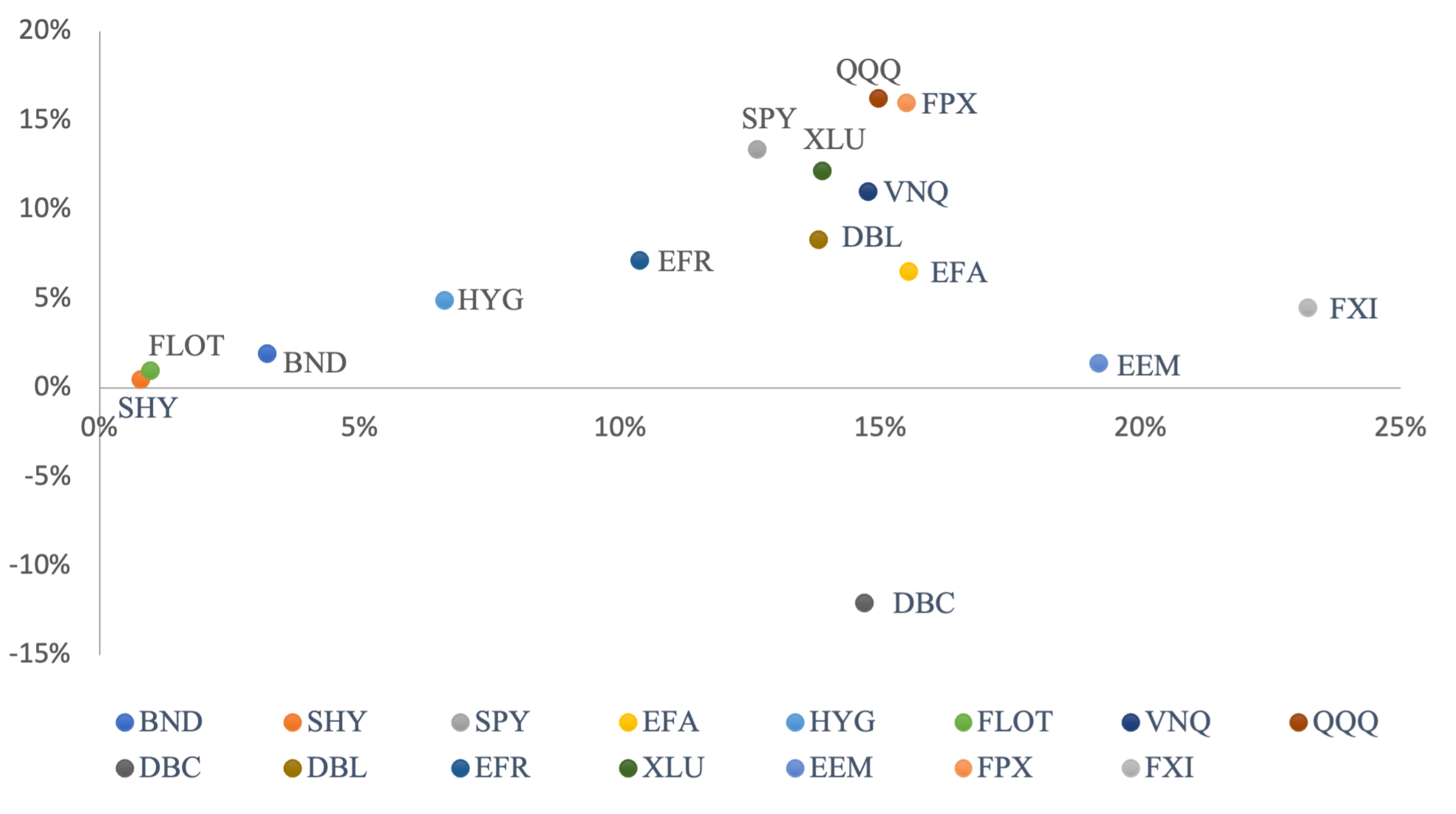
Figure 3.
Mean-variance representation of all portfolios and their relationship with the efficient frontier.
Figure 3.
Mean-variance representation of all portfolios and their relationship with the efficient frontier.
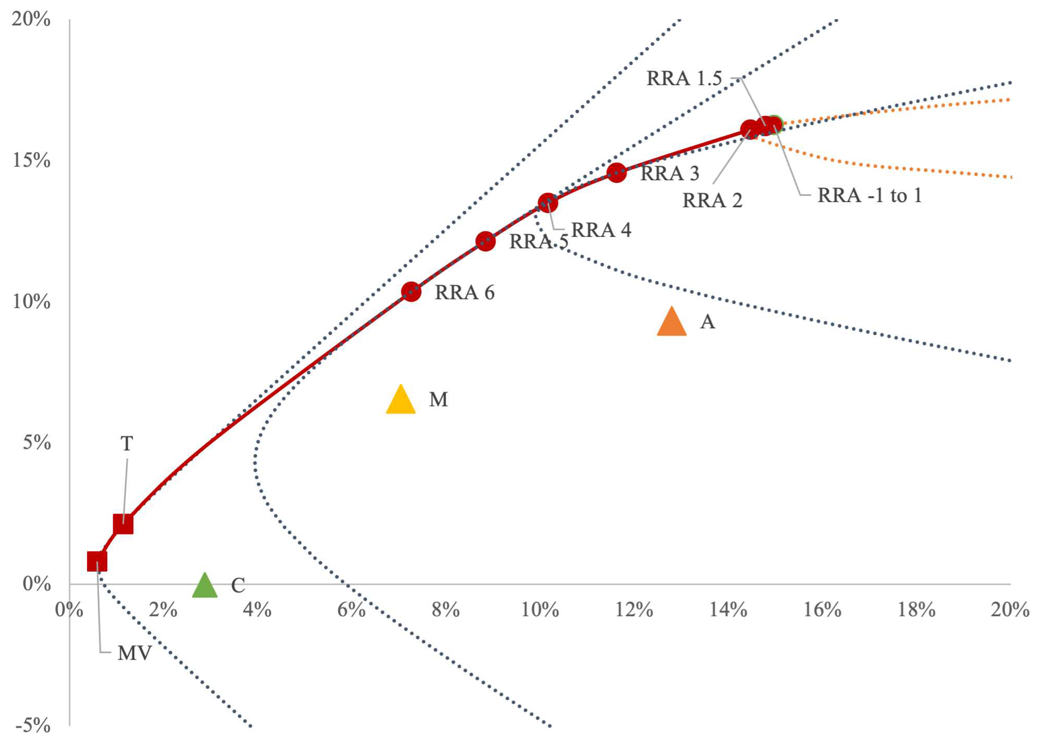
Figure 4.
Out-of-sample evolution of all portfolios.
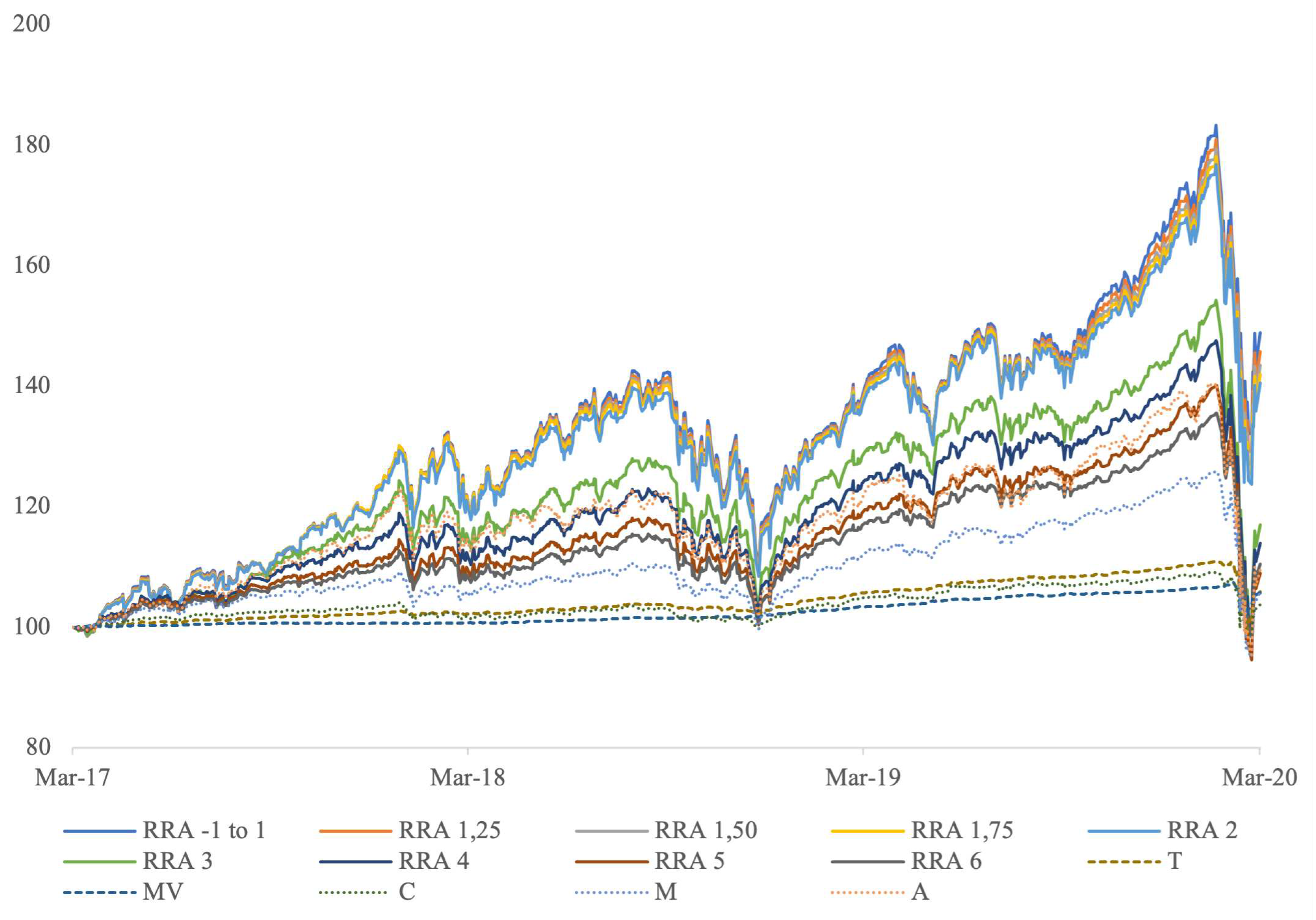
Table 1.
Description, abbreviations and categories of the 15 ETFs provided by the Riskalyze platform, which are used for the calculations in this study.
Table 1.
Description, abbreviations and categories of the 15 ETFs provided by the Riskalyze platform, which are used for the calculations in this study.
| INDEX | DESCRIPTION | CATEGORY |
| BND | Vanguard Total Bond Market ETF | Intermediate-Term Bond |
| SHY | iShares 1-3 Year Treasury Bond | Short Government |
| SPY | SPDR S&P 500 ETF | Large Blend |
| EFA | iShares MSCI EAFE | Foreign Large Blend |
| HYG | iShares iBoxx $ High Yield Corporate Bd | High Yield Bond |
| FLOT | iShares Floating Rate Bond | Ultrashort Bond |
| VNQ | Vanguard REIT ETF | Real Estate |
| QQQ | PowerShares QQQ ETF | Large Growth |
| DBC | PowerShares DB Commodity Tracking ETF | Commodities Broad Basket |
| DBL | Doubleline Opportunistic Credit Fund | Close-Ended Fixed Income Mutual Fund |
| EFR | Eaton Vance Senior Floating-Rate Fund | Close-Ended Fixed Income Mutual Fund |
| XLU | Utilities Select Sector SPDR ETF | Utilities |
| EEM | iShares MSCI Emerging Markets | Diversified Emerging Markets |
| FPX | First Trust US IPO ETF | Exchange Traded Fund |
| FXI | iShares China Large-Cap | Exchange Traded Fund |
Table 2.
Compositions and basic statistics on the following portfolios: tangent (T), minimum variance (MV), homogeneous (H) and Riskalize conservative (C), moderate (M), and aggressive (A).
Table 2.
Compositions and basic statistics on the following portfolios: tangent (T), minimum variance (MV), homogeneous (H) and Riskalize conservative (C), moderate (M), and aggressive (A).
| T | MV | H | C | M | A | |
|---|---|---|---|---|---|---|
| BND | 13.03% | 0.00% | 6.67% | 35.00% | 25.00% | 0.00% |
| SHY | 25.78% | 61.81% | 6.67% | 30.00% | 1.00% | 0.00% |
| SPY | 4.20% | 0.64% | 6.67% | 13.00% | 13.00% | 26.00% |
| EFA | 0.00% | 0.00% | 6.67% | 5.00% | 15.00% | 20.00% |
| HYG | 0.00% | 0.00% | 6.67% | 5.00% | 7.00% | 0.00% |
| FLOT | 51.37% | 37.05% | 6.67% | 5.00% | 0.00% | 0.00% |
| VNQ | 0.00% | 0.00% | 6.67% | 2.00% | 10.00% | 12.00% |
| QQQ | 0.00% | 0.00% | 6.67% | 0.00% | 5.00% | 17.00% |
| DBC | 0.00% | 0.00% | 6.67% | 0.00% | 5.00% | 7.00% |
| DBL | 1.13% | 0.00% | 6.67% | 0.00% | 7.00% | 0.00% |
| EFR | 1.32% | 0.05% | 6.67% | 0.00% | 7.00% | 0.00% |
| XLU | 0.00% | 0.00% | 6.67% | 0.00% | 5.00% | 0.00% |
| EEM | 0.00% | 0.00% | 6.67% | 0.00% | 0.00% | 7.00% |
| FPX | 3.17% | 0.44% | 6.67% | 0.00% | 0.00% | 6.00% |
| FXI | 0.00% | 0.00% | 6.67% | 0.00% | 0.00% | 5.00% |
| 2.14% | 0.82% | 6.21% | -0.02% | 6.57% | 9.32% | |
| 1.14% | 0.59% | 8.23% | 2.88% | 7.04% | 12.80% | |
| SR | 1.732 | 1.126 | 0.735 | -0.0609 | 0.9099 | 0.7158 |
Table 3.
Compositions and basic statistics on optimal MVT portfolios for investors with RRA = {−1, 0, 0.5, 1, 1.25, 1.5, 2, 3, 4, 5, 6}
Table 3.
Compositions and basic statistics on optimal MVT portfolios for investors with RRA = {−1, 0, 0.5, 1, 1.25, 1.5, 2, 3, 4, 5, 6}
| BND | 0.00% | 0.00% | 0.00% | 0.00% | 0.00% | 0.00% | 0.00% | 0.00% | 0.00% | 2.94% | 20.36% |
| SPY | 0.00% | 0.00% | 0.00% | 0.00% | 0.00% | 0.00% | 0.00% | 37.98% | 35.41% | 29.39% | 25.70% |
| QQQ | 100% | 100% | 100% | 100% | 91.63% | 85.76% | 76.63% | 0.00% | 0.00% | 0.00% | 0.00% |
| DBL | 0.00% | 0.00% | 0.00% | 0.00% | 0.00% | 0.00% | 0.00% | 0.00% | 13.38% | 15.89% | 12.47% |
| EFR | 0.00% | 0.00% | 0.00% | 0.00% | 0.00% | 0.00% | 0.00% | 0.00% | 0.00% | 10.35% | 8.89% |
| XLU | 0.00% | 0.00% | 0.00% | 0.00% | 0.00% | 0.00% | 2.79% | 11.70% | 14.33% | 14.12% | 9.65% |
| FPX | 0.00% | 0.00% | 0.00% | 0.00% | 8.37% | 14.24% | 20.58% | 50.32% | 36.87% | 27.31% | 22.93% |
| 16.27% | 16.27% | 16.27% | 16.27% | 16.25% | 16.23% | 16.10% | 14.57% | 13.51% | 12.15% | 10.36% | |
| 14.96% | 14.96% | 14.96% | 14.96% | 14.85% | 14.79% | 14.47% | 11.62% | 10.16% | 8.84% | 7.26% | |
| SR | 1.077 | 1.077 | 1.077 | 1.077 | 1.0836 | 1.0871 | 1.1022 | 1.2400 | 1.3136 | 1.3569 | 1.4045 |
Table 4.
Annual evolution of $ 100 investment.
| Portfolio | 29.03.2018 | 29.03.2019 | 30.03.2020 |
| RRA -1.00 – 1.00 | 122.01 | 138.07 | 148.85 |
| RRA 1.25 | 121.88 | 137.62 | 145.68 |
| RRA 1.5 | 121.79 | 137.30 | 143.48 |
| RRA 1.75 | 121.72 | 137.07 | 141.93 |
| RRA 2 | 121.11 | 136.56 | 140.57 |
| RRA 3 | 115.61 | 128.34 | 117.02 |
| RRA 4 | 112.39 | 123.85 | 113.95 |
| RRA 5 | 109.99 | 118.97 | 108.96 |
| RRA 6 | 108.75 | 116.87 | 110.43 |
| T | 102.25 | 105.69 | 105.93 |
| MV | 100.74 | 103.43 | 105.70 |
| H | 109.14 | 113.76 | 104.62 |
| C | 101.89 | 104.96 | 103.71 |
| M | 106.04 | 111.82 | 105.77 |
| A | 114.77 | 121.19 | 109.61 |
Table 5.
Out-of-sample performance of the various portfolios, ranked by Sharpe ratio.
| Portfolios | SR | ||
| MV | 1.84% | 0.03 | 0.8493 |
| RRA -1.00 –1.00 | 13.21% | 0.23 | 0.5859 |
| RRA 1.25 | 12.49% | 0.23 | 0.5617 |
| RRA 1.5 | 11.99% | 0.23 | 0.5440 |
| RRA 1.75 | 11.63% | 0.23 | 0.5309 |
| RRA 2 | 11.31% | 0.22 | 0.5257 |
| RRA 3 | 11.31% | 0.22 | 0.5257 |
| T | 1.91% | 0.05 | 0.4483 |
| C | 1.21% | 0.05 | 0.3315 |
| RRA 6 | 3.29% | 0.14 | 0.2693 |
| RRA 4 | 4.33% | 0.18 | 0.2620 |
| M | 1.86% | 0.12 | 0.1975 |
| RRA 5 | 2.85% | 0.17 | 0.1974 |
| A | 3.05% | 0.19 | 0.1871 |
| H | 1.50% | 0.13 | 0.1520 |
Disclaimer/Publisher’s Note: The statements, opinions and data contained in all publications are solely those of the individual author(s) and contributor(s) and not of MDPI and/or the editor(s). MDPI and/or the editor(s) disclaim responsibility for any injury to people or property resulting from any ideas, methods, instructions or products referred to in the content. |
© 2023 by the authors. Licensee MDPI, Basel, Switzerland. This article is an open access article distributed under the terms and conditions of the Creative Commons Attribution (CC BY) license (http://creativecommons.org/licenses/by/4.0/).
Copyright: This open access article is published under a Creative Commons CC BY 4.0 license, which permit the free download, distribution, and reuse, provided that the author and preprint are cited in any reuse.


