LP-based Row Generation using Optimization-based Sorting Method for Solving Budget Allocation with a Combinatorial Number of Constraints

Preprint

Article

LP-based Row Generation using Optimization-based Sorting Method for Solving Budget Allocation with a Combinatorial Number of Constraints

Altmetrics

Downloads

Views

Comments

A peer-reviewed article of this preprint also exists.

Aphisak Witthayapraphakorn

Sasarose Jaijit^*,Peerayuth Charnsethikul

Aphisak Witthayapraphakorn

Sasarose Jaijit^*,Peerayuth Charnsethikul

This version is not peer-reviewed

Submitted:

02 November 2023

Posted:

02 November 2023

You are already at the latest version

Alerts

Abstract

A novel approach was developed that combined LP-based row generation with optimization-based sorting to tackle computational challenges posed by budget allocation problems with combinatorial constraints. The proposed approach dynamically generated constraints using row generation and prioritized them using optimization-based sorting to ensure a high-quality solution. Computational experiments and case studies revealed that as the problem size increased, the proposed approach outperformed simplex solutions in terms of solution search time. Specifically, for a problem with 50 projects (N = 50) and 2,251,799,813,685,250 constraints, the proposed approach found a solution in just 1.4 seconds, while LP failed due to the problem size. The proposed approach demonstrated enhanced computational efficiency and solution quality compared to traditional LP methods.

Keywords:

Subject: Computer Science and Mathematics - Computational Mathematics

1. Introduction

Budget allocation problems, commonly referred to as capital budgeting problems often involve many constraints. These constraints typically consist 2^N investment patterns, which further increase to 2✕(2^N-1) patterns when considering upper and lower bounds. Consequently, efficiently and effectively solving these problems becomes increasingly challenging, particularly when considering the total number of projects represented by N. Traditional optimization techniques may struggle to handle the combinatorial explosion of constraints, often resulting in time-consuming computations and no guarantee of optimal solutions within a reasonable timeframe. However, recent advancements in linear programming-based row generation and optimization-based sorting methods offer promising solutions to address these challenges.

Linear programming (LP) provides a powerful framework for modeling and solving optimization problems with linear constraints. By formulating the budget allocation problem as an LP model, decision-makers can systematically allocate resources to various activities while considering multiple objectives and constraints [1,2,3]. However, when faced with many combinatorial constraints, the traditional LP formulation may become computationally intractable.

An innovative approach combines linear programming-based row generation to overcome this challenge. Row generation involves iteratively generating new constraints (rows) added to the problem formulation, effectively expanding the solution space and refining the solution quality [4]. By iteratively adding constraints that are most relevant to the current solution, the row generation process enables efficient exploration of the combinatorial constraint space.

Furthermore, optimization-based sorting methods enhance the row-generation process by incorporating sorting algorithms tailored to the specific constraints and objectives of the budget allocation problem. This algorithm employs intelligent search strategies to efficiently discover the optimal solutions. With a focus on practical applications, the optimization-based sorting method has demonstrated the ability to generate optimal solutions within a reasonable timeframe [5,6].

The combination of linear programming-based row generation and optimization-based sorting methods offers a powerful approach to solving budget allocation problems with a combinatorial number of constraints. This integrated methodology allows decision-makers to handle large-scale optimization problems, allocate resources efficiently, and identify optimal budget allocation strategies.

This study also is aimed to explore and analyze the proposed method. It delves into the theoretical foundations of these related techniques, highlights their advantages and challenges, and discusses their practical implementation. Randomly generated structural problems are examined to illustrate both the efficiency or effectiveness and potential of this approach in complex budget allocation scenarios.

By leveraging the capabilities of linear programming-based row generation and optimization-based sorting, decision-makers can make informed budget allocation decisions, optimize resource utilization, and achieve superior financial outcomes. The proposed methodology holds immense promise for organizations facing complex budget allocation challenges, enabling them to navigate the intricate landscape of constraints and make strategic resource allocation decisions.

2. Literature Review

Budget allocation problems with combinatorial constraints are complex optimization models originating from the study by Weingartner [7], which has found applications in various fields such as resource allocation and project planning. Linear programming (LP) is a widely used technique to solve such problems efficiently. However, when dealing with a large number of constraints, the computational complexity of LP becomes time-consuming to solve. This literature review explores the application of row-generation techniques to enhance the efficiency of solving budget allocation problems with combinatorial constraints using sorting methods.

Row generation, a sub-technique within Benders decomposition, is a powerful approach initially proposed by Unger [8,9], which offers an application for solving large-scale LP problems in budget allocation. It focuses on generating a subset of constraints, known as "rows," dynamically during the optimization process. Hummeltenberg [10], Zak [11], Muter et al. [12], Muter and Sezer [13] and Witthayapraphakorn et al. [14] consistently highlight the advantages of employing a row generation algorithm that incorporates a warm-start strategy and an approximation scheme, surpassing the performance of linear programming, particularly in scenarios involving a substantial number of constraints. These compelling findings affirm the efficacy of row-generation technique as an effective approach for addressing linear programming problems characterized by a comprehensive set of constraints. According to the literature reviews over the past decade, a limited number of studies have investigated the application of row-generating techniques in the context of budget allocation problems; however, notable research by Fard et al. [15] has contributed to this area. Their study presents a model employing the bender decomposition method for budgeting purposes within international humanitarian organizations and provides analytical insights into the optimal solution. Additional scholarly studies employ the row generation method to allocate various types of resources, such as energy [16] and location [17,18].

The possibility of utilizing effective heuristic methods to generate initial starting points in combinatorial optimization motivates the exploration of applying sorting techniques, specifically in budget allocation problems known for their exceptional efficiency in identifying feasible solutions [19]. Sorting is a technique that aims to prioritize constraints based on their potential impact on the solution quality. This approach involves assigning weights or scores to constraints and ordering them in a way that maximizes the likelihood of finding a feasible solution quickly. Sorting has been successfully employed in various allocation problems. For example, Song and Mu [20] proposes a heuristic algorithm based on assignment to solve the sequence sorting problem of large-scale automated storage requests in multiple input/output (multi-I/O) depots. The proposed algorithm considers equivalent merging and minimum cost merging methods of subloops to eliminate subloops emerged in the sorting process. Their proposed algorithm offers a solution to optimize the sequence of storage requests in multi-I/O depots, which can improve efficiency and cost-effectiveness in practice. Weiner et al. [21] provide valuable insights into the utilization of sorting in subproblems optimization and highlight its potential for solving large-scale mixed integer programs (MIPs). Specifically, their research demonstrates the effective utilization of machine learning (ML) for ranking constraint relaxations of MIPs. Their proposed method outperforms existing heuristic and ML-based methods in terms of solution quality and computational time. The authors suggest that their approach has the potential to be applied to other optimization problems beyond MIPs.

The feasibility of using row generation methods (i.e., Benders decomposition) is hindered by the complexity of combinatorial constraints and the limited time availability for solution generation. Consequently, the utilization of sorting techniques is motivated by the intricate nature of combinatorial constraints, while also taking into account the potential implementation of row-generation methods within the available computational time and the problem size to be solved. The current literature on budget allocation problems lacks evidence supporting the effectiveness of combining heuristics and LP approaches (i.e., integer programming, Benders decomposition, and row generation) in achieving optimal solutions. Moreover, studies in related fields, like location-allocation and network allocation, provide insights into the comparative speed of solution discovery using mixed methods. Fischetti et al. [22] demonstrate the practical effectiveness and straightforward implementation of their proposed approach, which applies Benders decomposition to solve the facility allocation master problem with non-separable subproblems. By employing a simple sorting application on Benders cut, their study showcases the successful application of generalized Benders cuts for convex problems. Furthermore, numerous studies have explored alternative heuristics beyond sorting to identify optimal solutions in combination with the Benders decomposition method. For example, Maher [23] reveals how large neighborhood search heuristics can enhance Benders decomposition algorithms and improve mixed-integer programming solvers. Costa and Gendron [24], Maheo et al. [25], and Oliveira et al. [26] employ heuristic techniques, such as branch-and-cut, local search, Pareto-optimal cuts, and multiple cuts, to generate additional cuts when solving the master problem through Benders decomposition. Their respective studies focus on fixed-charge network design [24], bin allocation for waste management [25], and multiple allocation hub network design [26].

The review provides a comprehensive overview of the evolution in budget allocation or capital budgeting research, transitioning from traditional linear programming and row generation to the utilization of diverse heuristic approaches, specifically focusing on the utilization of sorting algorithms. Our main contribution to this study represents in the implementation of linear programming-based row generation using optimization-based sorting methods for budget allocation problems. The study compares the efficiency of solution-finding, measured in terms of time, by employing the linear programming, row generation method, and a hybrid approach combining row generation and sorting. Through computational experiments and case studies, we have demonstrated the advantages of this combined approach and proved whether employing sorting methods will yield equivalent results with binary programming or integer programming techniques, particularly when compared to the conventional row generation method and linear programming. Further elaboration on our proposed approach can be found in Section 3, Section 4, Section 5, Section 6 and Section 7. Section 3 introduces problem structures and notations. Section 4 applies row generation to solve the budget allocation model. Section 5 demonstrates the application of sorting methods in the row-generation process. Section 6 proves the optimal solutions derived from sorting methods. Finally, Section 7 showcases the model's application in solving budget allocation problems.

3. Problem Structures and Notations

The problem structure of budget allocation involves determining how available budget resources should be allocated among different projects within an organization or government entity, considering factors such as maximizing profits and constraint-based resource limitations. When making investment decisions for each project, there are two options: invest or not invest. This results in a total of 2^N possible patterns, considering all projects N. Furthermore, when considering budget allocation within the investment boundaries as lower and upper bounds, there are a total of 2✕(2^N-1) combinatorial constraints to be considered. Efficiently solving large problems involves employing the principle of row generations while considering maximum and minimum total investments for project groups. Furthermore, utilizing the sorting method to rank constraints enhances problem-solving efficiency through row generation.

The proposed approach for budget allocation, following the structure described by Sangkhasuk et al. [27], can be stated as:

The objective is to maximize the overall benefits obtained from allocating budget resources among the different projects.
Each project receives a budget allocation proportional to its potential benefits, with allocations not exceeding 1.
The total budget allocation across all projects is limited to a maximum of 1.
Combinatorial constraints consist of 2✕(2^N-1) constraints, where N represents the number of projects.
Each investment pattern has a lower and upper boundary of each constraint that is proportional to the amount of investment. For instance, if there are 5 projects, an investment pattern must allocate between 0.1 to 0.8 of the investment, resulting in N-1 boundary values.

The notations in order to formulate the above model are as follows:

Z: Objective function, which aims to maximize the benefits obtained from an investment.
c_j: Benefits obtained from investment project j based on the allocated funds.
x_j: Decision variable, which is the proportion of investment in project j.
a_ij: Allocated investment pattern i in project j (j = 1, 2, …, N), where a_ij = 1 or 0.
N: Total number of projects.
U_k: Upper bound constraint set on the proportion of investment in k projects.
L_k: Lower bound constraint set on the proportion of investment in k projects.
u_k: Proportional investment for a total number of allocated investment projects used to create the upper bound constraint of investment in Equation (2), where u_k < u_k+1 and 0 < u_k < 1.
l_k: Proportional investment for a total number of allocated investment projects used to create the lower bound constraint of investment in equation (3), where l_k < u_k and l_k < l_k+1 and 0 < l_k < 1.

The mathematical model (1)-(5) is used for budget allocation problems as follows:

Max Z = \sum_{j = 1}^{N} c_{j} x_{j}

(1)

subject to

\sum_{j = 1}^{N} a_{i j} x_{j} \leq U_{k}, i = 1, 2, \dots, 2^{N} - 1

(2)

\sum_{j = 1}^{N} a_{i j} x_{j} \geq L_{k}, i = 1, 2, \dots, 2^{N} - 1

(3)

\sum_{j = 1}^{N} x_{j} \leq 1

(4)

0 \leq x_{j} \leq 1

(5)

where the values of

U_{k}

and

L_{k}

are related to the total number of allocated investment projects k.

The objective function (1) is formulated to optimize investment profits. The upper (

U_{k}

) bound (2) and lower (

L_{k}

) bound (3) serve to establish boundaries for the investment pattern. In this particular context, binary sequences are employed to conveniently represent investment patterns, with 1 indicating funding and 0 denoting a lack of funding. For example, the funding patterns of five projects can be represented as 0 1 0 0 0 or 1 0 0 0 0. To ensure that the cumulative investment proportions assigned to the funded projects do not exceed 1, constraint (4) is imposed. This constraint guarantees that the total investment remains within the available budgets. Additionally, constraint (5) imposes a restriction on the investment proportion, confining it within the range of 0 to 1. Table 1 presents the values of variables

u_{k}

and

l_{k}

in constraints (2) and (3) respectively, which are dependent on the total number of allocated investment projects.

4. Row Generation Applied to Solving Budget Allocation Model

The utilization of the row generation method in the context of the budget allocation problem encompasses three distinctive sub-models, which consist of:

Mathematical model for relaxed budget allocation;
Row generation applied to the upper bound model;
Row generation applied to the lower bound model.

4.1. Sub-Model 1: Mathematical Model for Relaxed Budget Allocation

Introduce relaxations to account for flexibility in the budget allocation process. Relaxations allow for partial allocations or fractional allocations of the budget. Instead of using binary variables, we may allow fractional values for decision variables. This enables allocating a portion of the budget to multiple alternatives, allowing for more fine-grained resource allocation. The mathematical model for relaxed investment allocation incorporates the objective function (1) and constraints (4) and (5), with constraints (2) and (3) substituted by constraints (6) and (7) respectively,

\sum_{j = 1}^{N} a_{r j}^{U} x_{j} \leq U_{k}, r = 1, 2, \dots, R,

(6)

\sum_{j = 1}^{N} a_{r j}^{L} x_{j} \geq L_{k}, r = 1, 2, \dots, R,

(7)

where the

a_{r j}^{U}

and

a_{r j}^{L}

represent the upper and lower bounds of investment in project j for round r of solution finding, the initial solution is obtained by utilizing the objective function (1), and constraints (4) and (5) during the first round (r = 0). Subsequently, constraints (6) and (7) are incrementally added in each subsequent round until the most feasible and optimal solution is achieved at round R, where

R \leq 2^{N} - 1

4.2. Sub-Model 2: Row Generation Applied to the Upper Bound Constraint

By iteratively generating new constraints, row generation refines the mathematical model and progressively narrows down the feasible solution space. The lower bound is gradually improved by finding better feasible solutions at each iteration, while the upper bound is tightened by adding new constraints to the model. This process continues until the optimal solution is obtained or until the termination criterion is satisfied. Specifically, in the case of row generation for the upper bound model, the mathematical model can be expressed as follows:

Max T_{k}^{U} = \sum_{j = 1}^{N} a_{j k}^{* U} x_{j}^{* r - 1} - U_{k},

(8)

subject to

\sum_{j = 1}^{N} a_{j k}^{* U} = k

(9)

a_{j k}^{* U} = {0, 1}

(10)

k = 1, \dots, N - 1

(11)

where the

T_{k}^{U}

is the target value, in an unconventional form, represents the objective of finding an investment pattern that violates the upper limit constraint under k investment projects,

a_{j k}^{* U}

is the decision variable for investing in project j in case of allocating k investment projects that violates the highest upper limit constraint,

x_{j}^{* r - 1}

is a constant obtained from finding the value of

x_{j}

in the mathematical model for capital budgeting under relaxed conditions in the previous round r-1, and k is the sum of the number of investment projects with a value ranging from 1 to N-1.

The model described in (8)-(11) is utilized to generate constraints (6) in round r. The objective function (8) aims to identify an investment pattern that surpasses the upper limit constraint the most among k investment projects. Constraint (9) outlines the requirement for investing in k investment projects. Constraint (10) determines the decision of investing or not in project j, given the allocation of k investment projects. Constraint (11) ensures that all potential solutions are iterated for N-1 rounds using the objective function (8) under constraints (9) and (10). The value of

a_{j k}^{* U}

that yields the highest positive value of

T_{k}^{U}

is then then transferred to

a_{r j}^{U}

in constraint (6).

4.3. Sub-Model 3: Row Generation Applied to the Lower Bound Constraint

During row generation for the lower bound constraint, the feasible solution space undergoes further refinement, integrating stricter constraints and narrowing down the range of potential solutions. This iterative process facilitates the exploration of various allocations and enhances resource optimization, taking into account the lower bound. The model for this process are as follows:

Min T_{k}^{L} = \sum_{j = 1}^{N} a_{j k}^{* L} x_{j}^{* r - 1} - L_{k},

(12)

subject to

\sum_{j = 1}^{N} a_{j k}^{* L} = k,

(13)

a_{j k}^{* L} = {0, 1},

(14)

k = 1, \dots, N - 1,

(15)

where the

T_{k}^{L}

is the target value with the objective of violating the lowest upper bound investment format under k investment projects,

a_{j k}^{* L}

is the decision variable for investing in project j in the case where there is investment in project k, which violates the lower bound constraint the most, and k is the total number of investment projects with a value ranging from 1 to N-1.

The model represented in (12) to (15) is utilized for generating the constraints (7) in round r. The objective function (12) is designed to identify the investment pattern in project k that maximally violates the lower bound constraint. Constraint (13) establishes the investment constraint for project k. Constraint (14) determines the investment status of project j when project k is being investment. Constraint (15) sets the condition for exploring all possible solutions in N-1 rounds by the objective function (12) under constraints (12) to (14). Subsequently, it assigns the value of

a_{j k}^{L}

that yields the lowest negative value of

T_{k}^{L}

a_{r j}^{L}

in in constraint (7).

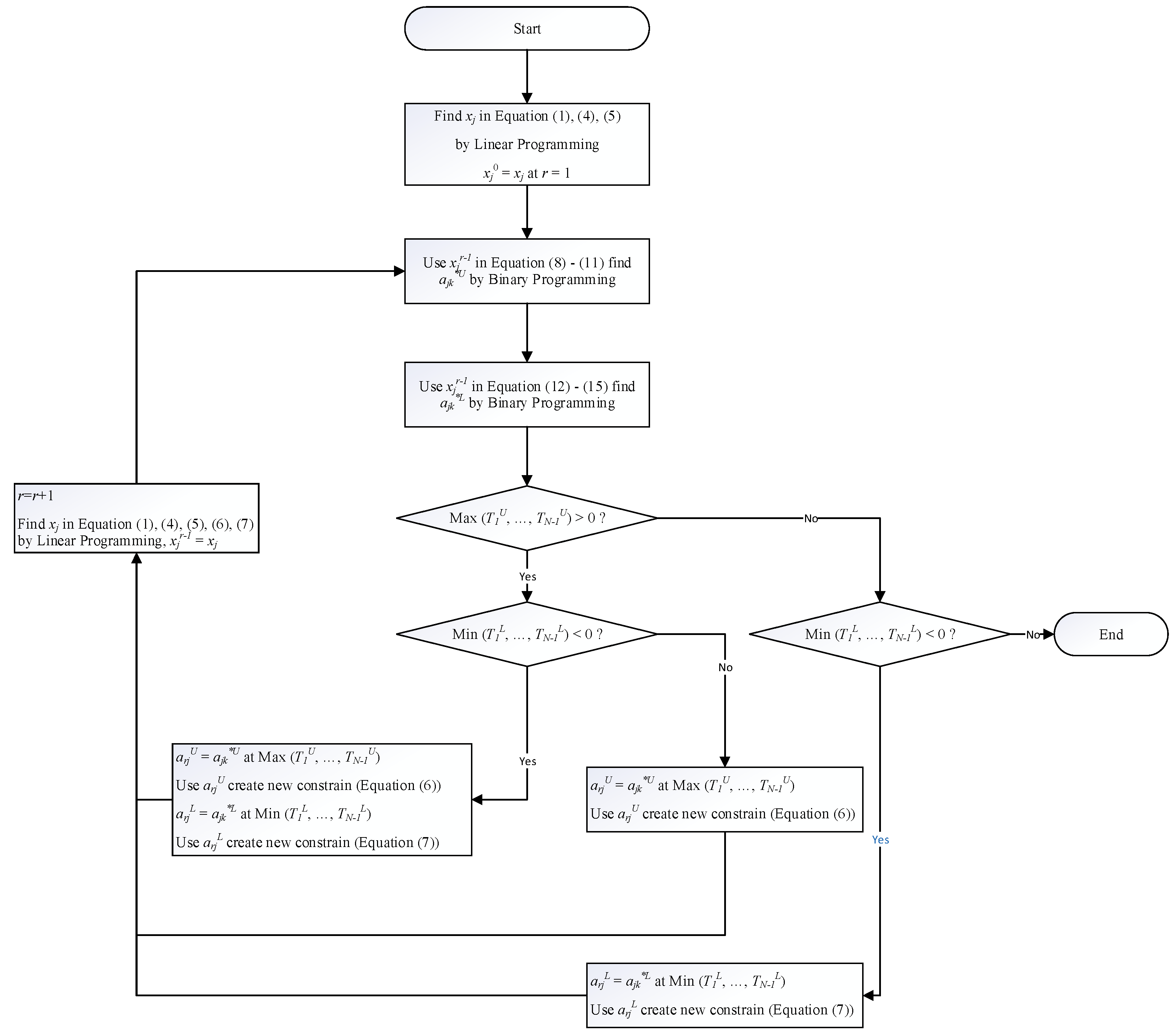
The working process of row generation applied to solving the budget allocation model, using three sub-models, can be summarized concisely based on the steps outlined in Figure 1. The specific details of each step are as follows:

Step 1: Find the value of $x_{j}$ in round r = 1 using linear programming with equations (1), (4), and (5), then set $x_{j}^{* 0}$ = $x_{j}$ ;
Step 2: Use $x_{j}^{* r - 1}$ and equations (8)-(11) to find the value of $a_{j k}^{* U}$ using binary programming;
Step 3: Use $x_{j}^{* r - 1}$ and equations (12)-(15) to find the value of $a_{j k}^{* L}$ using binary programming;
Step 4: Check the values of Max( $T_{1}^{U}$ , $T_{2}^{U}$ ,…, $T_{N - 1}^{U}$ ) and Min( $T_{1}^{L}$ , $T_{2}^{L}$ ,…, $T_{N - 1}^{L}$ ), and separate into four conditions:

Max( $T_{1}^{U}$ , $T_{2}^{U}$ ,…, $T_{N - 1}^{U}$ ) > 0 and Min( $T_{1}^{L}$ , $T_{2}^{L}$ ,…, $T_{N - 1}^{L}$ ) < 0, proceed to Step 5;

Max( $T_{1}^{U}$ , $T_{2}^{U}$ ,…, $T_{N - 1}^{U}$ ) > 0 and Min( $T_{1}^{L}$ , $T_{2}^{L}$ ,…, $T_{N - 1}^{L}$ ) ≥ 0, proceed to Step 6;

Max( $T_{1}^{U}$ , $T_{2}^{U}$ ,…, $T_{N - 1}^{U}$ ) ≤ 0 and Min( $T_{1}^{L}$ , $T_{2}^{L}$ ,…, $T_{N - 1}^{L}$ ) < 0, proceed to Step 7;

Max( $T_{1}^{U}$ , $T_{2}^{U}$ ,…, $T_{N - 1}^{U}$ ) ≤ 0 and Min( $T_{1}^{L}$ , $T_{2}^{L}$ ,…, $T_{N - 1}^{L}$ ) ≥ 0, proceed to Step 9;
Step 5: Set $a_{r j}^{U}$ = $a_{j k}^{* U}$ , where $a_{j k}^{* U}$ is the set of answers for Max( $T_{1}^{U}$ , $T_{2}^{U}$ ,…, $T_{N - 1}^{U}$ ), then use $a_{r j}^{U}$ to create equation (6). Set $a_{r j}^{L}$ = $a_{j k}^{* L}$ , where $a_{j k}^{* L}$ is the set of answers for Min( $T_{1}^{L}$ , $T_{2}^{L}$ ,…, $T_{N - 1}^{L}$ ), then use $a_{r j}^{L}$ to create equation (7). Proceed to Step 8;
Step 6: Set $a_{r j}^{U}$ = $a_{j k}^{* U}$ , where $a_{j k}^{* U}$ is the set of answers for Max( $T_{1}^{U}$ , $T_{2}^{U}$ ,…, $T_{N - 1}^{U}$ ), then use $a_{r j}^{U}$ to create equation (6). Proceed to Step 8;
Step 7: Set $a_{r j}^{L}$ = $a_{j k}^{* L}$ , where $a_{j k}^{* L}$ is the set of answers for Min( $T_{1}^{L}$ , $T_{2}^{L}$ ,…, $T_{N - 1}^{L}$ ), then use $a_{r j}^{L}$ to create equation (7). Proceed to Step 8;
Step 8: Adjust the value of r=r+1, find the value of $x_{j}$ in round r using Linear Programming with equations (1), (4), (5), (6), and (7), then set $x_{j}^{* r - 1}$ = $x_{j}$ . Return to Step 2;
Step 9: stops the search for solutions, with $x_{j}$ being the final solution set that provides the best result. The entire process of the 9 steps can be summarized as shown in Figure 1.

5. Application of Sorting Method in Row Generation Process

The row generation process in the budget allocation model incorporates a sorting method that utilizes descending order sorting for determining

a_{j k}^{* U}

from equations (8)-(11), and ascending order for determining

a_{j k}^{* L}

from equations (12)-(15). This sorting method is utilized as an alternative to binary programming in order to derive the solutions for

a_{j k}^{* U}

and

a_{j k}^{* L}

variables during steps 2 and 3 of the row generation process outlined in Section 4. The sorting technique proposed by Witthayapraphakorn et al. [11] is adopted, although its effectiveness in yielding the maximum value of

T_{k}^{U}

for all values of k and absence of lower boundary conditions is yet to be formally proven. Consequently, this section focuses on explaining the procedure for obtaining the solution for

T_{k}^{L}

. The proof demonstrating that the sorting method attains the maximum value of

T_{k}^{U}

for all values of k is presented in Section 6. The proof employs a case-by-case approach similar to that used for

T_{k}^{L}

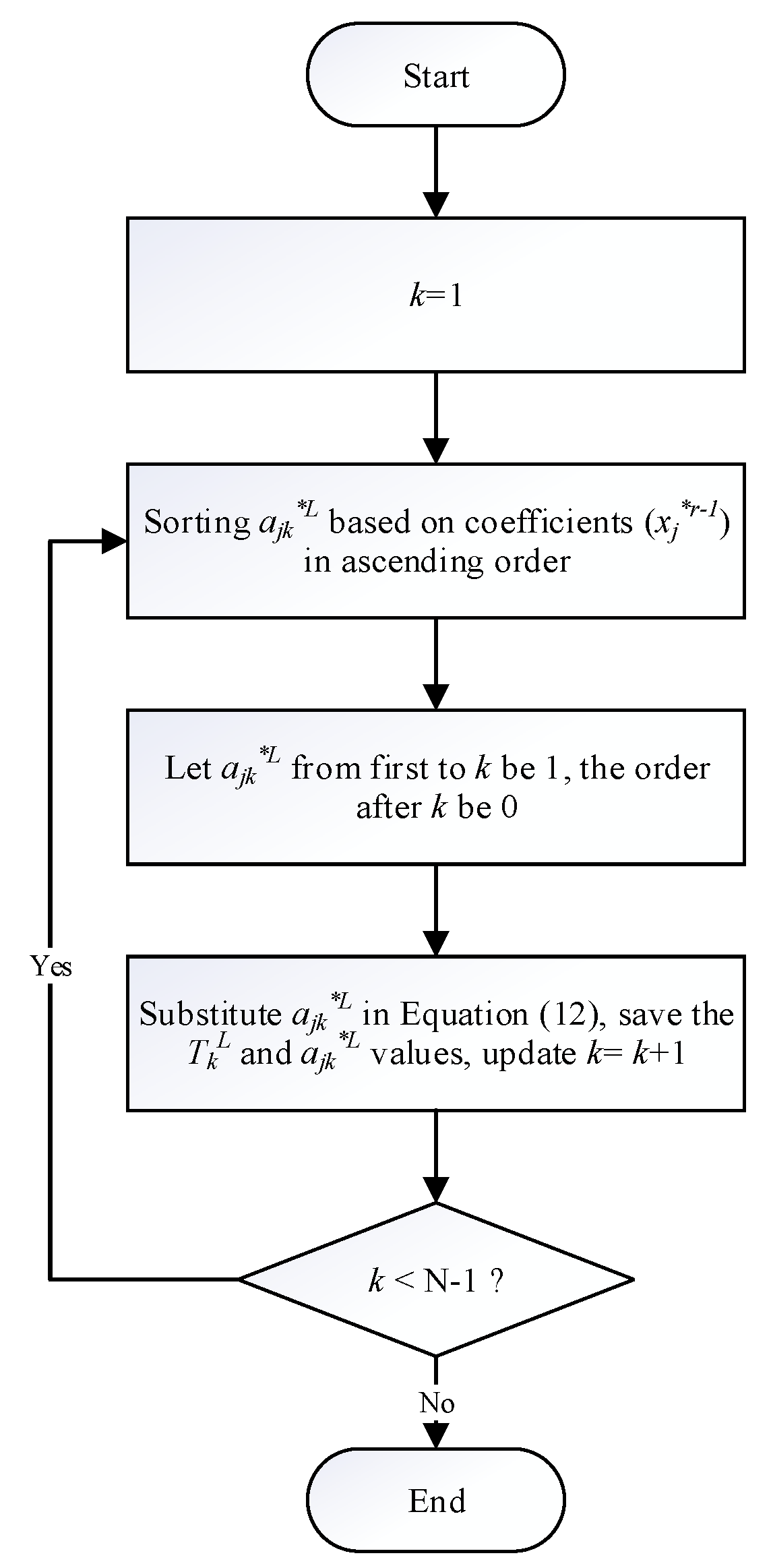
, but modified to demonstrate the attainment of the minimum value instead of the maximum value. The steps for the sorting method, aiming to minimize the value of

a_{j k}^{* L}

, are presented concisely in Figure 2. The following are the detailed explanations for each step:

Step 1: Set k = 1;
Step 2: Sort $a_{j k}^{* L}$ in ascending order using the value of $x_{j}^{* r - 1}$ ;
Step 3: Set $a_{j k}^{* L}$ 1 for the first k elements and 0 for the remaining elements;
Step 4: Compute $T_{k}^{L}$ using equation (12) with the updated values of $a_{j k}^{* L}$ , and record the value of $T_{k}^{L}$ and $a_{j k}^{* L}$ . update k = k+1;
Step 5: Check if k < N-1. If true, go to Step 2; otherwise, go to Step 6;
Step 6: End the process and return the values of $T_{k}^{L}$ and $a_{j k}^{* L}$ for use in the Row Generation process.

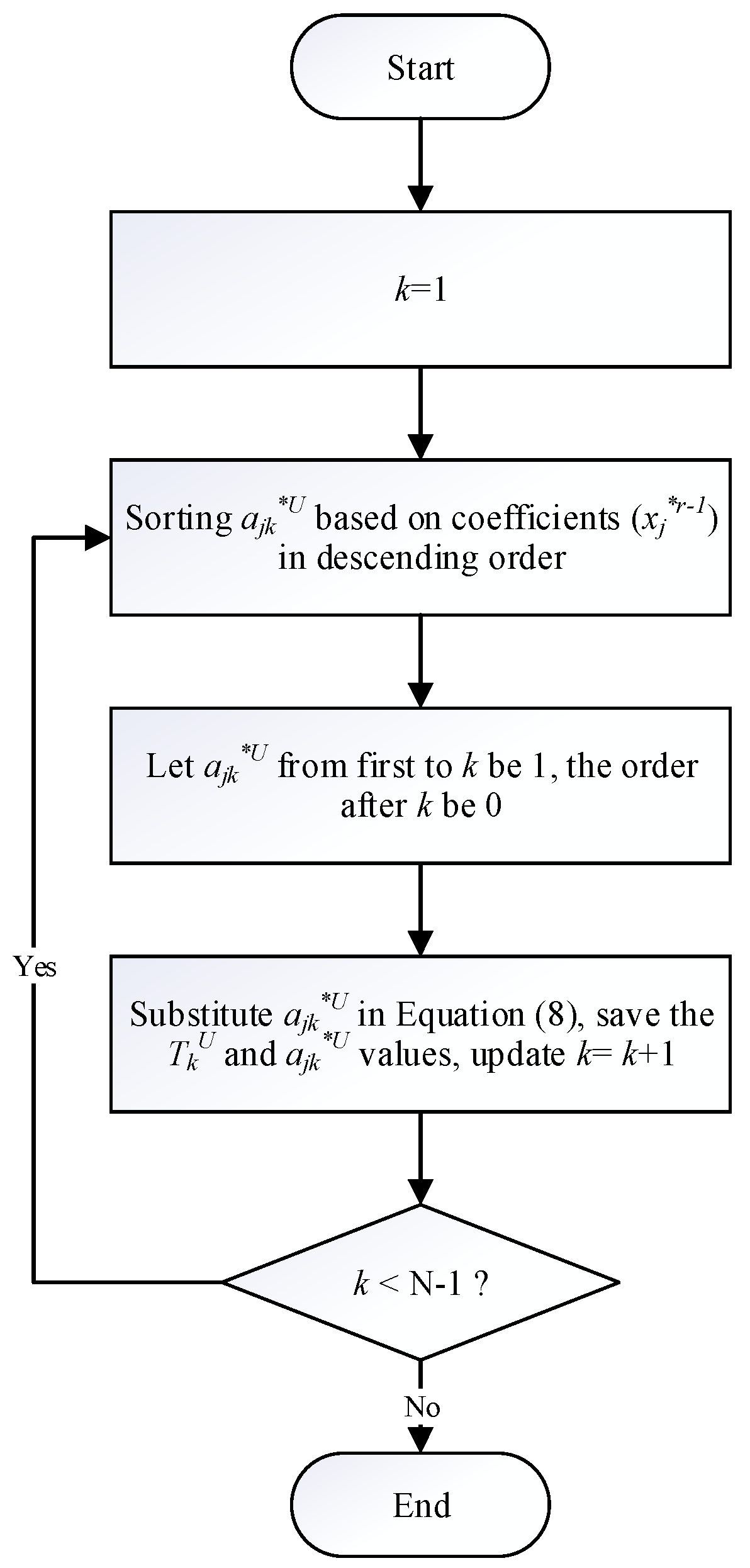
For determining the value of

a_{j k}^{* U}

, a comparable methodology to that presented in Figure 2 will be employed, with the exception that step 2 will involve sorting in descending order, and step 4 will entail determining the value of

T_{k}^{U}

using equation (8). A comprehensive overview of the entire procedure is depicted in Figure 3.

6. Proving Optimal Solutions Derived from Sorting Methods

In this section, our objective is to provide a proof of optimality for the sorting method presented in Figure 3, specifically in determining the optimal value of

T_{k}^{U}

for any feasible solution

a_{k}^{* U}

. We aim to demonstrate that the value obtained from the sorting method is greater than or equal to the value of

T_{k}^{U}

obtained from

a_{k}^{* U}

Let

a_{k}^{* U}

represent an arbitrary feasible solution. Without loss of generality, we assume that the coefficients

x_{j}^{* r - 1}

are sorted in descending order as b(j), following the prescribed sorting method.

Consider any k = 1, 2, ..., N-1. According to the sorting method, we assign

a_{j k}^{* U}

= 1 to the k largest coefficients in b, denoted by b(j), while setting

a_{j k}^{* U}

= 0 for the remaining coefficients. Let S denote the set of indices corresponding to the k largest coefficients in b, defined as S = {j: b(j) belongs to the k largest coefficients in b}. Consequently, we have

a_{j k}^{* U}

= 1 for j ∈ S, and

a_{j k}^{* U}

= 0 for j ∉ S.

Subsequently, we proceed to calculate the value of

T_{k}^{U}

for the solution obtained through the sorting method:

T_{k}^{U} = b (1) a_{1 k}^{* U} + b (2) a_{2 k}^{* U} + \dots + b (N) a_{N k}^{* U} = b (1) + b (2) + \dots b (k)

The rationale behind the final step is based on the fact that

a_{j k}^{* U}

is assigned a value of 1 for j ∈ S, where S represents the indices corresponding to the k largest coefficients in b. This implies that the elements within S are indeed the k largest coefficients in b.

Moving forward, let us now proceed to compute

T_{k}^{U}

for the arbitrary solution

a_{k}^{* U}

T_{k}^{U} = x_{1}^{* r - 1} a_{1 k}^{* U} + x_{2}^{* r - 1} a_{2 k}^{* U} + \dots + x_{N}^{* r - 1} a_{N k}^{* U} = \sum (x_{j}^{* r - 1} \times a_{j k}^{* U}),

T_{k}^{U}

= ∑(

x_{j}^{* r - 1}

), for j ∈ S (because

a_{j k}^{* U}

= 1 for j ∈ S) + ∑(

x_{j}^{* r - 1}

), for j ∉ S (because

a_{j k}^{* U}

= 0 for j ∉ S).

Since

x_{j}^{* r - 1}

is sorted in descending order as b(j), we have b(j) ≥

x_{j}^{* r - 1}

for all j. Therefore:

\sum (x_{j}^{* r - 1}), for j \in S \leq \sum (b (j)), for j \in S, \sum (x_{j}^{* r - 1}), for j \notin S \leq \sum (b (j)), for j \notin S .

By combining the aforementioned inequalities, we obtain the following expression:

T_{k}^{U} = \sum (x_{j}^{* r - 1}), for j \in S + \sum (x_{j}^{* r - 1}, for j \notin S \leq \sum (b (j)), for j \in S + \sum (b (j)), for j \notin S = \sum (b (j)) = T_{k}^{U} (from the sorting method)

It has been demonstrated that the value of

T_{k}^{U}

obtained from the sorting method solution is greater than or equal to the value derived from any alternative feasible solution

a_{k}^{* U}

. Consequently, the sorting method yields an optimal solution.

In order to establish the validity of the sorting method presented in Figure 2, we can employ a similar proof approach as previously used, wherein we demonstrate the minimization of the obtained value and subsequently apply the sorting method in ascending order.

7. Computational Studies

This section applies the proposed approach to exemplify a budget allocation problem, and compares the solving time among three methods: linear programming, row generation, and the proposed model (row generation using an optimization-based sorting method: ROS).

7.1. Experimental Model

The experiments are conducted using Matlab Version R2022b with Computer Spec Processor Intel(R) Core(TM) i7-7700 3.60GHz, RAM 32.0 GB solving by linprog function for linear programming and intlinprog for binary programming.

The experiments are conducted in two parts:

Comparison of processing time for all three methods with project sizes ranging from 5 to 20 projects, with one additional project added for each iteration;
Comparison of processing time for row generation and ROS methods for larger problem sizes, with project sizes ranging from 5 to 50 projects, with an additional 5 projects added for each iteration.

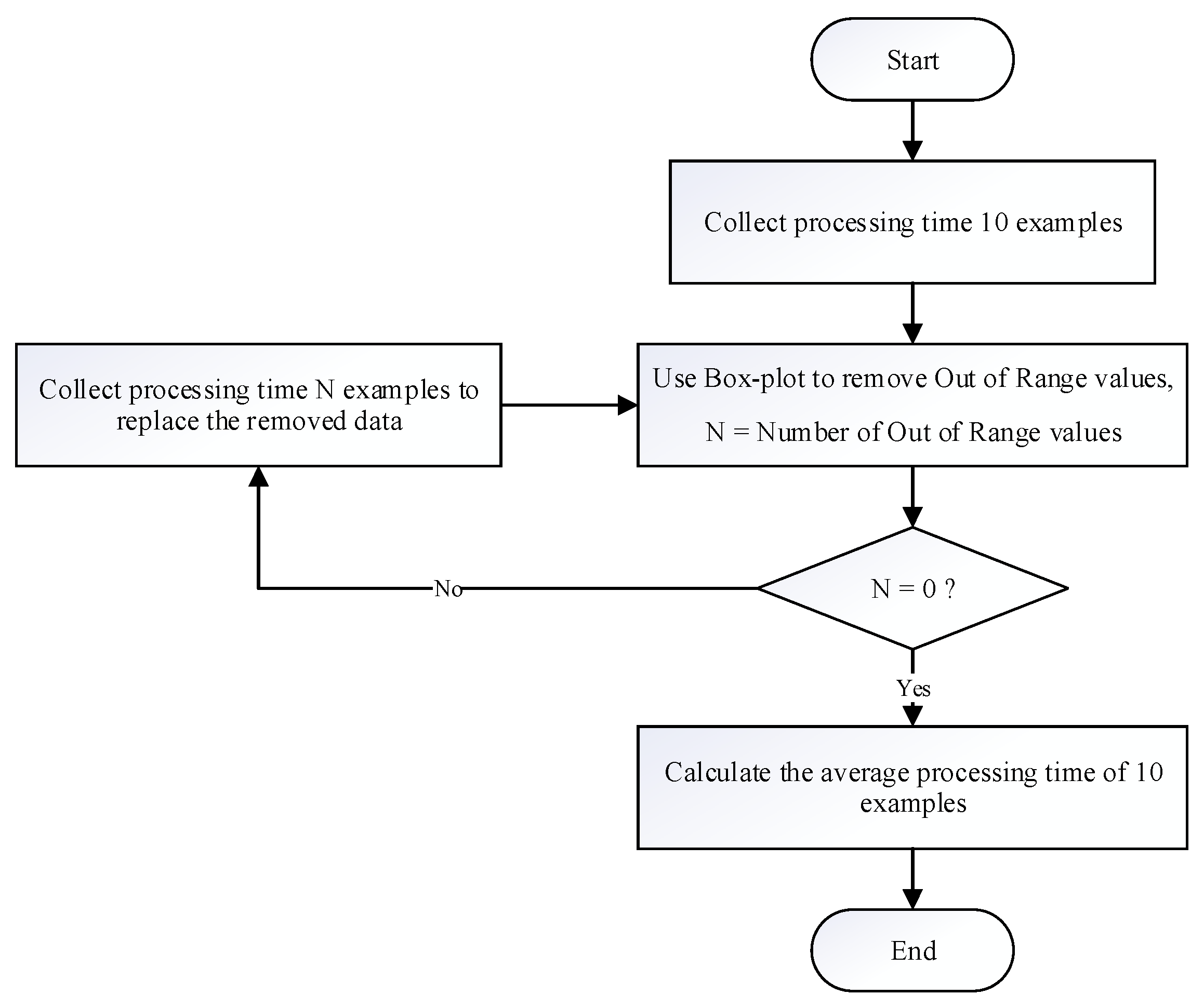
To gather data on processing time, the initial 10 examples were recorded, and any outliers were eliminated through the utilization of box plots. Subsequently, further data was acquired until no outliers remained, and the average processing time was computed. The process is visually presented in Figure 4.

7.2. Experimental Results

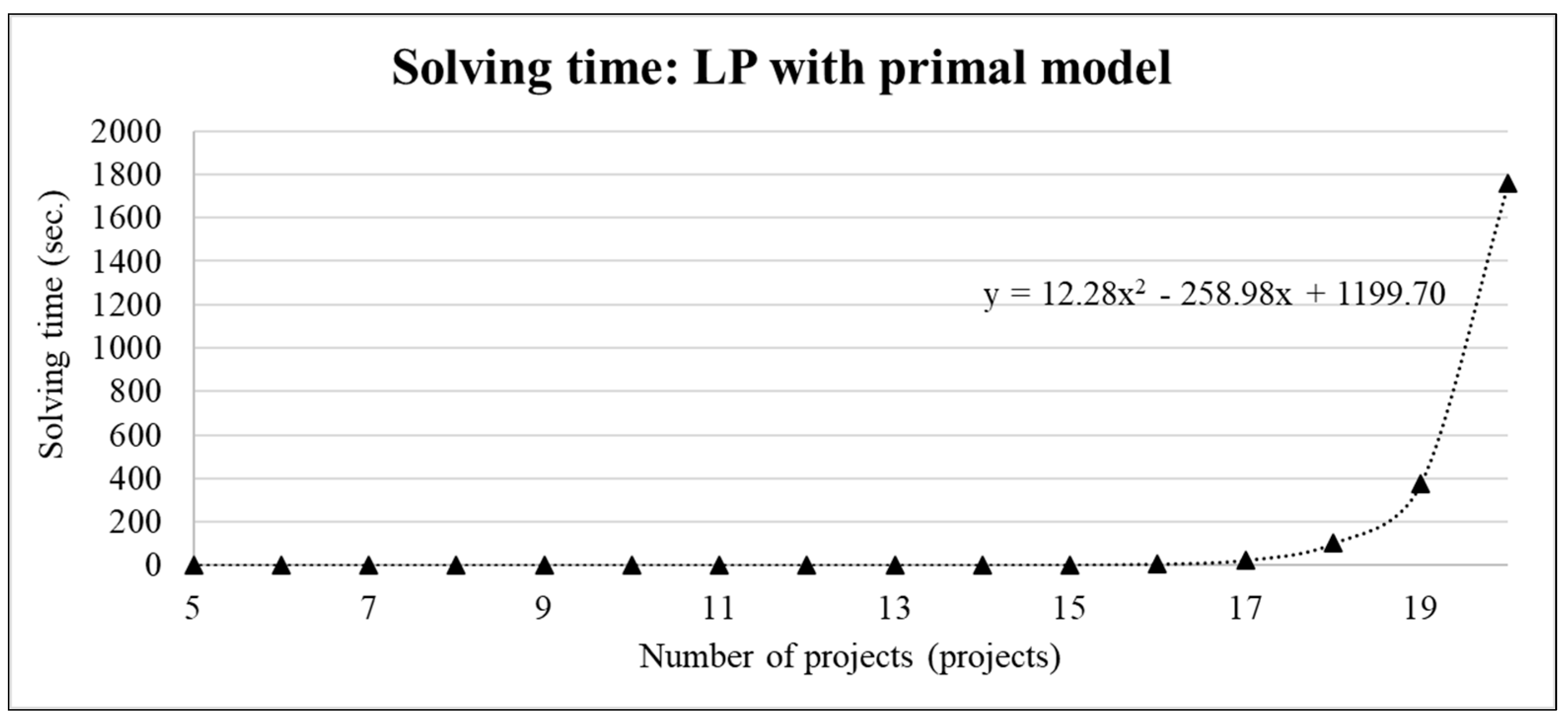
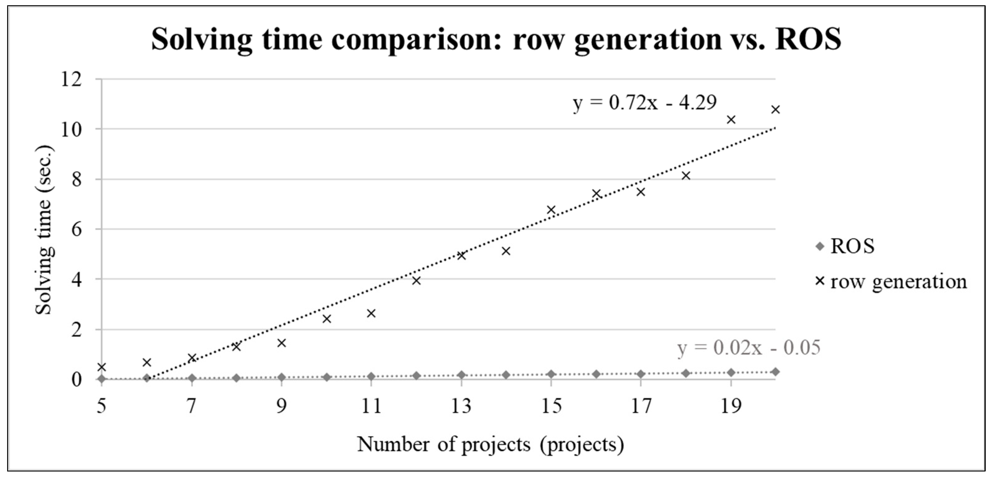
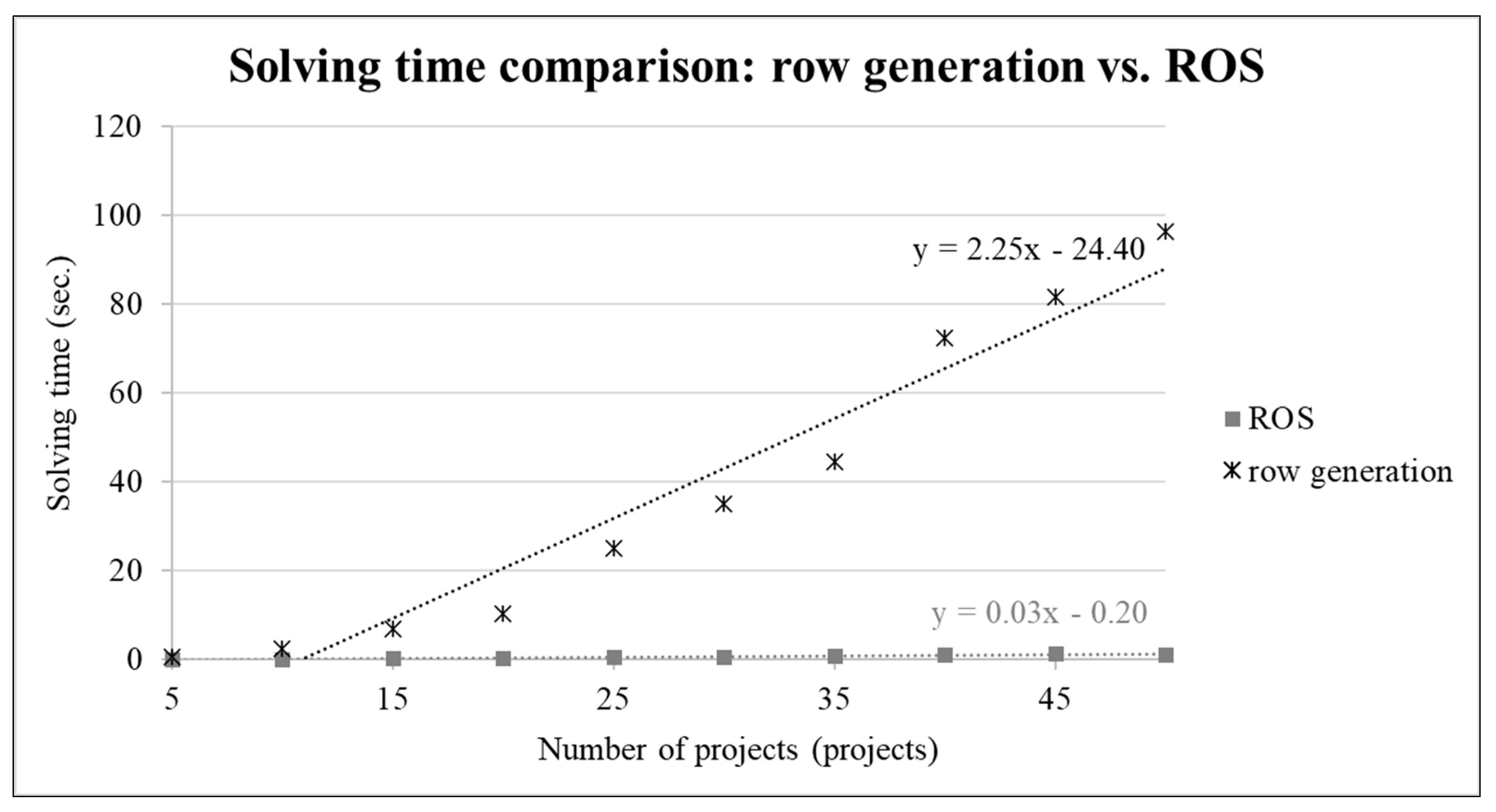
The experimental results encompassed a comparative analysis of processing time among three distinct methods, with a division based on problem sizes. These problem sizes consisted of two ranges: 1) a range spanning from 5 to 20 projects, and 2) a range spanning from 5 to 50 projects. Figs. 5 and 6 exhibit the outcomes of the processing time comparison for problem sizes ranging from 5 to 20 projects and 5 to 50 projects, respectively.

Based on the findings presented in Figure 5 and Figure 6, it can be observed that for problem sizes ranging from 5 to 9 projects, the linear programming approach utilizing the primal model outperforms all other methods in terms of speed. However, for larger problem sizes (11 projects or more), the ROS method exhibits superior processing time compared to the linear programming model. Furthermore, when comparing the row generation method with the ROS method, the ROS method consistently demonstrates faster performance. This can be attributed to the fact that sorting algorithms generally exhibit faster execution than binary programming methods when the problem entails identifying the optimal solution from a set of sortable values. Sorting facilitates the efficient determination of the minimum or maximum value within the set, which can serve as the solution to the problem [6]. To provide a more comprehensive visualization of the relationship between processing time and problem size, a graph was generated and is presented in Figure 5.

The analysis of Figure 5 reveals distinct relationships between processing time and problem size for different methods. Specifically, in the case of linear programming with the primal model, the processing time demonstrates an exponential increase with respect to problem size. Conversely, for the row generation and ROS methods, the processing time exhibits a linear pattern in relation to problem size. Notably, the ROS method exhibits a lower slope than the row generation method. To gain further insight and establish a clearer trend regarding the association between processing time and problem size for the row generation and ROS methods, an additional experiment was conducted.

Figure 5 visually represents the recorded time required for solving the optimization problem using linear programming with the primal model. The results highlight a substantial increase in solving time when dealing with 20 projects. However, it is worth noting that the findings do not include the solving time for 50 projects using this particular model. Moving to Figure 6, it can be observed that even with an increased problem size of 50 projects, both the row generation and ROS methods exhibit a consistent linear relationship with the problem size, similar to that observed with 20 projects. Notably, the graph depicting the ROS method demonstrates a less steep slope when compared to the graph representing the row generation method (Figure 7).

8. Conclusion

The budget allocation problem addressed in this study is a matrix-structured problem that becomes increasingly complex as the number of projects (N) increases. The traditional linear programming approach faces significant challenges due to the exponential growth of constraints, making it computationally expensive and impractical for larger problem sizes. To overcome this issue, the study proposes a novel solution using the principles of row generation and sorting method. The row generation technique incrementally adds constraints to the problem, eliminating the need to include all constraints upfront. This approach reduces complexity and improves computational efficiency. Additionally, the binary programming method traditionally used to create constraints is replaced with the sorting method, which proves to be faster and less complex for generating subproblems.

Experimental results demonstrate that the row-generation hybrid sorting method significantly decreases computation time compared to linear programming. For instance, when N = 20 with 2,097,150 constraints, the linear programming method takes an average computation time of 1,757.13 seconds, while the row generation hybrid sorting method only requires 0.30 seconds. Even when the problem size increases to N = 50 with 2,251,799,813,685,250 constraints, the row generation hybrid sorting method completes in just 1.4 seconds, while linear programming fails to find a solution due to the problem scales.

Comparisons among three methods, including linear programming with the primal model, row generation, and the ROS method, reveal valuable insights. Linear programming excels for smaller problem sizes but becomes inefficient for larger ones. The ROS method consistently demonstrates faster processing times compared to both linear programming and the row generation method. This efficiency can be attributed to the inherent advantages of sorting algorithms in finding optimal solutions among sorted values. The relationship between processing time and problem size is visualized in Figure 5 and Figure 6, indicating that linear programming exhibits a polynomial regression, while the row generation and ROS methods exhibit linear regressions. The ROS method shows a lower slope than the row generation method, signifying superior efficiency in scaling with increasing problem sizes.

Overall, the findings emphasize the significant time consumption associated with linear programming for larger problem sizes. In contrast, the row generation hybrid sorting method and the ROS method maintain a linear relationship with problem size and offer more efficient solutions. These valuable insights shed light on the comparative performance of different methods in terms of problem size and processing time, providing guidance for addressing similar matrix-structured problems, such as the Capital Budgeting problem explored in this research.

9. Further Research

Given equations 3 and 4, the careful assignment of values to U_k and L_k is crucial to avoid infeasible solutions. To address the potential for infeasibility, a two-stage LP (stochastic linear programming) approach can be employed, which helps mitigate the risk of constraint infeasibility. This involves introducing two types of variables into equations 3 and 4: corrective action variables and opportunity cost variables. However, it is important to note that incorporating these variables may significantly increase the model's complexity, resulting in a substantial growth in the number of variables to

2 \times 2^{N}

for each variable type, thereby leading to an LP model with an exceedingly large number of constraints and variables. This aspect opens avenues for future research and investigation.

Author Contributions

Conceptualization, A.W., S.J. and P.C.; methodology, A.W. and P.C.; software, A.W.; validation, A.W., S.J. and P.C.; formal analysis, A.W. and P.C.; investigation, A.W. and S.J.; resources, A.W.; data curation, A.W. and S.J.; writing—original draft preparation, A.W. and S.J.; writing—review and editing, A.W., S.J. and P.C.; visualization, A.W. and S.J.; supervision, P.C.; project administration, A.W. and S.J.; funding acquisition, A.W. and S.J. All authors have read and agreed to the published version of the manuscript.

Funding

This research received no external funding.

Data Availability Statement

Not applicable.

Acknowledgments

This study was supported by the Faculty of Engineering, University of Phayao, Thailand, and the Faculty of En-gineering at Kamphaeng Saen, Kasetsart University, Thailand.

Conflicts of Interest

The authors declare no conflict of interest.

References

Charnes, A.; Cooper, W.W.; Miller, M.H. Application of linear programming to financial budgeting and the costing of funds. J. Bus. 1959, 32, 20–46. [CrossRef]
Norris, W.T. Application of linear programming to financial budgeting and the costing of funds. Eng. Econ. 1960, 5, 55–56. [CrossRef]
Candler, W.; Boehlje, M. Use of linear programming in capital budgeting with multiple goals. Am. J. Agric. Econ. 1971, 53, 325–330. [CrossRef]
Benders, J.F. Partitioning procedures for solving mixed-variables programming problems. Numer. Math. 1962, 4, 238–252. [CrossRef]
Kalra, M.; Tyagi, S.; Kumar, V.; Kaur, M.; Mashwani, W.K.; Shah, H.; Shah, K. A comprehensive review on scatter search: techniques, applications, and challenges. Math. Probl. Eng. 2021, 2021, 1–21. [CrossRef]
Cormen, T.H.; Leiserson, C.E.; Rivest, R.L.; Stein, C. Introduction to Algorithms, 3rd ed.; The MIT Press: Massachusetts London, England, 2009; pp. 5–15.
Weingartner, H.M. Mathematical Programming and the Analysis of Capital Budgeting Problems, 1st ed.; Prentice Hall: Englewood Cliffs, New Jersey, 1963; pp. 139–157.
Unger, V.E. Capital budgeting and mixed zero-one integer programming. AIIE Trans. 1970, 2, 28–36. [CrossRef]
Unger, V.E. Duality results for discrete capital budgeting models. Eng. Econ. 1974, 19, 237–251. [CrossRef]
Hummeltenberg, W. Capital budgeting with benders decomposition. Eur. J. Oper. Res. 1985, 21, 318–329. [CrossRef]
Zak, E.J. Row and column generation technique for a multistage cutting stock problem. Comput. Oper. Res. 2002, 29, 1143–1156. [CrossRef]
Muter, I.; Birbil, S.I.; Bülbül, K. Benders decomposition and column-and-row generation for solving large-scale linear programs with column-dependent-rows. Eur. J. Oper. Res. 2018, 264, 29–45. [CrossRef]
Muter, I.; Sezer, Z. Algorithms for the one-dimensional two-stage cutting stock problem. Eur. J. Oper. Res. 2018, 271, 20–32. [CrossRef]
Witthayapraphakorn, A.; Thavorn, E.; Tippayasak, R.; Charnsethikul, P. Row generation technique to solve the problems of capital budgeting allocation under combinatorial constraints. TJOR 2018, 6, 10–21.
Fard, M.K.; Ljubić, I.; Papier, F. Budgeting in international humanitarian organizations. Manuf. Serv. Oper. Manag. 2021, 24, 1261–1885.
Qorbani, M.; Amraee, T. Long term transmission expansion planning to improve power system resilience against cascading outages. Electr. Power Syst. Res. 2022, 192, 1–7. [CrossRef]
Han, J.; Zhang, J.; Zeng, B.; Mao, M. Optimizing dynamic facility location-allocation for agricultural machinery maintenance using Benders decomposition. Omega 2021, 105, 102498. [CrossRef]
Karamyar, F.; Sadeghi, J.; Yazdi, M.M. A Benders decomposition for the location-allocation and scheduling model in a healthcare system regarding robust optimization. Neural. Comput. Appl. 2018, 29, 873–886. [CrossRef]
Shabaz, M.; Kumar, A. SA sorting: a novel sorting technique for large-scale data, Discrete. J. Comput. Netw. Commun. 2019, 2019, 1–7. [CrossRef]
Song, Y.B.; Mu, H.B. Large-scale storage/retrieval requests sorting algorithm for multi-I/O depots automated storage/retrieval systems. Discrete. Dyn. Nat. Soc. 2021, 2021, 1–16. [CrossRef]
Weiner, J.; Ernst, A.T.; Li, X.; Sun, Y. Ranking constraint relaxations for mixed integer programs using a machine learning approach. EURO J. Comput. Optim. [182023, 11, 1–29. [CrossRef]
Fischetti, M.; Ljubić, I.; Sinnl, M. Benders decomposition without separability: a computational study for capacitated facility location problems. Eur. J. Oper. Res. 2016, 253, 557–569. [CrossRef]
Maher, S.J. Enhancing large neighbourhood search heuristics for Benders’ decomposition. J. Heuristics 2021, 27, 615–648. [CrossRef]
Costa, A.M.; Gendron, B. Accelerating Benders decomposition with heuristic master problem solutions. Pesqui. Operacional. 2012, 32, 3–20. [CrossRef]
Mahéo, A.; Rossit, D.G.; Kilby, P. A Benders decomposition approach for an integrated bin allocation and vehicle routing problem in municipal waste management. Eur. J. Oper. Res. 2021, 1408, 3–18. [CrossRef]
Oliveira, F.A. de Sá, E.M.; de Souza, S.R. Benders decomposition applied to profit maximizing hub location problem with incomplete hub network. Comput. Oper. Res. 2022, 142, 1–22. [CrossRef]
Sangkhasuk, R.; Vivithkeyoonvong, T.; Phuangchampee, B.; Anurak, S.; Leartsiriphesaj, S.; Charnsethikul, P. Capital budgeting problem with combinatorial allocation constraints by column generation method. TJOR 2020, 8, 37–48.

Figure 1. Application of Row Generation in the Capital Budgeting Model.

Figure 2. Applying the Sorting Method to find

a_{j k}^{* L}

in Row Generation.

Figure 2. Applying the Sorting Method to find

a_{j k}^{* L}

in Row Generation.

Figure 3. Applying the Sorting Method to find

a_{j k}^{* U}

in Row Generation.

Figure 3. Applying the Sorting Method to find

a_{j k}^{* U}

in Row Generation.

Figure 4. The method for collecting processing time data.

Figure 5. Solving time of LP with primal model for 5-20 projects.

Figure 6. Solving time comparison between row generation and ROS method for 5-20 projects.

Figure 7. Solving time comparison between row generation and ROS method for 5-50 projects.

Table 1. Relationship between U_k and L_k with the total number of allocated investment projects.

$\sum_{j = 1}^{N} a_{i j}$	U_k	L_k
1 2 ⋮ k ⋮ N-1	u₁ u₂ ⋮ u_k ⋮ u_N-1	l₁ l₂ ⋮ l_k ⋮ l_N-1

Disclaimer/Publisher’s Note: The statements, opinions and data contained in all publications are solely those of the individual author(s) and contributor(s) and not of MDPI and/or the editor(s). MDPI and/or the editor(s) disclaim responsibility for any injury to people or property resulting from any ideas, methods, instructions or products referred to in the content.

© 2023 by the authors. Licensee MDPI, Basel, Switzerland. This article is an open access article distributed under the terms and conditions of the Creative Commons Attribution (CC BY) license (http://creativecommons.org/licenses/by/4.0/).

Copyright: This open access article is published under a Creative Commons CC BY 4.0 license, which permit the free download, distribution, and reuse, provided that the author and preprint are cited in any reuse.

MDPI Initiatives

Important Links

Choose an area of interest and we will send you notifications of new preprints at your preferred frequency.

Disclaimer

LP-based Row Generation using Optimization-based Sorting Method for Solving Budget Allocation with a Combinatorial Number of Constraints

Abstract

1. Introduction

2. Literature Review

3. Problem Structures and Notations

4. Row Generation Applied to Solving Budget Allocation Model

4.1. Sub-Model 1: Mathematical Model for Relaxed Budget Allocation

4.2. Sub-Model 2: Row Generation Applied to the Upper Bound Constraint

4.3. Sub-Model 3: Row Generation Applied to the Lower Bound Constraint

5. Application of Sorting Method in Row Generation Process

6. Proving Optimal Solutions Derived from Sorting Methods

7. Computational Studies

7.1. Experimental Model

7.2. Experimental Results

8. Conclusion

9. Further Research

Author Contributions

Funding

Data Availability Statement

Acknowledgments

Conflicts of Interest

References

MDPI Initiatives

Important Links

Subscribe