1. Introduction
WSNs consist of nodes capable of sensing, signal processing, and communicating. In addition to object detection, the inherent property of control and activation in WSNs is also of interest [
1]. One of the most significant applications of WSNs is moving targets classification in designated areas, which is an important signal processing task and has found widespread civilian applications such as intelligent transportation system [
2] and real-time traffic surveillance [
3].
Multi-targets classification in WSN has been a difficult problem, for multi-target classification methods, one is to extend on the binary classification algorithm; such as DAGSVM method [
4], one-against-all SVM (OAA-SVM) method [
5], binary-tree SVM [
6] method, the hierarchical binary tree multi-class SVM (BTMSVM) method [
7]. Another type of multi-target classifiers based on neural network approach is also one of the most popular classification methods in recent years. Wang, Y (Wang, Yan) [
8] et al. proposed a powerset fusion network(PFN) method to classify moving targets using acoustic-vibrational signal features. Xu, TH (Xu, Tonghua) [
9] et al. used the parallel recurrent neural network(PRNN) method to classify vibrating targets. Belsare, K (Belsare, Karan) [
10] et al. have created a convolution neural network (CNN) trained using pre processed data for feature extraction andwaste image classification in WSN.
In addition to this, Kim, Y[
11] prosposed Gaussian mixture model (GMM) algorithm for node-level target classification in WSN, and utilized the classification and regression tree (CART) algorithm to improve the accuracy.Zhao, Q[
12] et al. proposed an improved independent vector analysis (IVA) method based on a microphone array for acoustic signal enhancement in the wild.
The limited storage space and computing capacity of the WSN node hinder the implementation of the complex of classification algorithm on the node's chip. For example, even when running on a computer, HSMC-SVM algorithm takes 5S-7S to classify 1397 data using trained classifiers [
13] and LST-KSVC takes about 73S to classify 5000 data [
14]. For WSN nodes, the complexity of the mentioned methods are sufferable.
In this paper ,we proposes a multi-DBN weighted voting classification algorithmon the basis of the Deep Belief Network (DBN)[
15] classifier, and implemented it on the nodes of the WSN monitoring system by means of "upper training, lower transplantation" appraoch. The new algorithm aims at improving the accuracy of target classification while rendering the increment of the computational complexity acceptable.
The rest of the paper is organized as follows. After introducing After introducing the feature extraction method, wavelet coefficient energy rate (WCER) method [
16], and dataset utilized for validating the proposed method.
Section 2 elaborates on the composition and principles of the DBN classifier.
Section 3 introduces the proposed multi-DBN weighted voting algorithm for moving target classification in details. Based on this,
Section 4 describes how to transplant the algorithm to resource-limited WSN nodes. The performance of the method is discussed in
Section 5.
Section 6 concludes the paper.
2. Deep Belief Network classifier
DBN is a neural network architecture includes several restricted Boltzmann machines (RBM) [
17]. The concept of deep neural networks has been proposed for some time. Prior to 2006, researchers observed that the impact of deep networks was inferior to that of shallow networks, and training was challenging. However, it has not been studied in depth until Hinton [
18] introduced unsupervised feature learning to overcome this difficulty that it began to be more comprehensively investigated. The DBN method, which incorporates both deep learning and feature learning, has since garnered considerable attention. Since Hinton's pioneering work in image processing using DBN networks, deep learning has become increasingly prominent in a range of signal and information processing domains.
The DBN classifier is a neural network that is trained using sample feature data and their corresponding category labels. The mapping relationship between the sample feature data and corresponding category labels is fitted by a multilayer DBN network. This fitted mapping relationship is then used to to process the feature data to be classified to achieve the purpose of classifying the target.
2.1. Principles of Deep Belief Networks
DBN is a type of deep neural network that comprises multiple unsupervised Restricted Boltzmann Machines (RBM) layers and one supervised back-propagation network (BP) layer[
19]. The lowest level neurons in DBN are responsible for receiving input data vectors and transforming them through RBM into the hidden layer. As a result, the higher-layer RBM's input data comes from the lower-layer RBM's output. In this section, we will begin by presenting the architecture and principles behind Restricted Boltzmann Machines (RBM), which serves as the fundamental building block for Deep Belief Networks (DBN). Subsequently, we will delve into the specifics of DBN's architecture and comprehensive training process.
2.1.1. Restricted Boltzmann Machine (RBM)
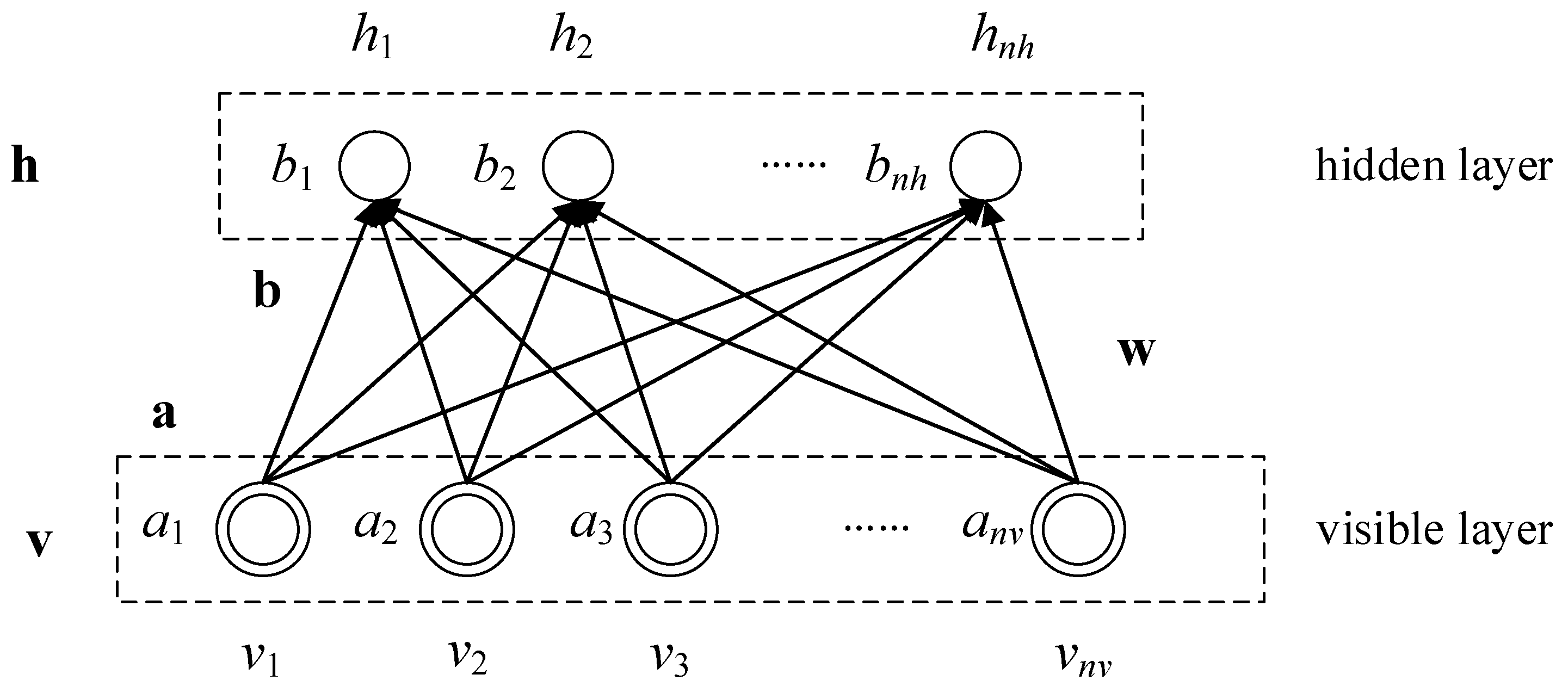
The Restricted Boltzmann Machine (RBM) is a neural network consisting of two layers. The first layer is known as the visible or input layer, while the second layer is known as the hidden layer. Both layers contain multiple neurons, and the neurons in the visible layer are connected to those in the hidden layer. Importantly, there is no connection between neurons within each layer, nor is there any intra-layer communication.
Figure 1 illustrates the basic structure of the RBM model.
where the visible layer is denoted as v, with nv neurons (v1 , v2 ,..., vnv ) ; h represents the hidden layer with nh hidden neurons (b1 , b2 ,..., bnh ). The bias of the neurons in the visible layer is denoted as a with the values of (a1 , a2 ,..., anv ); The bias of the neurons in the hidden layer is denoted as b, and their values are (b1 , b2 ,..., bnh ). w denotes the weight coefficients between the visible layer neurons and the hidden layer neurons.
During the training process of a neural network, an error function is defined to represent the difference between the network output and sample labels. The error function is then continuously decreased monotonically by adjusting network parameters throughout the network according to the gradient in order to obtain acceptable parameters for the network as a whole. Different in RBM, the energy function
E(
v,
h) is employed to represent the total system energy in its current state, as depicted in Equation (1). During the training process of restricted Boltzmann machines (RBM), the objective is to achieve the system's global minimum energy. To accomplish this, the network weights are initially changed randomly. Then, the network's energy function is calculated after the modification. If the network's energy is reduced, the change in weights is accepted; otherwise, this change was accepted according to a predetermined probability distribution. This approach is similar to the simulated annealing algorithm and aims to locate the global optimal solution.
where
θ is the RBM internal parameter, which is specifically {
a,
b,
w}.
Additionally, an energy probability model is defined in the RBM to depict the output of the neuron and the probabilistic connection between the network energy and parameters, which is demonstrated in the following equation:
where
Z is a normalization constant for the simulated physical system, obtained by summing the energy values between all visible and hidden layer units. The energy probability model is also the joint probability model of the visible and hidden layers, depicting the joint probability distribution of the outputs of the neurons in the visible layer
v and hidden layer
h when the energy of the RBM system is
E(
v,
h;
θ).
The independent distribution of the visual layer vector
v can be obtained from the following equation using the joint probability distribution provided by Eq. (3).
Eq(4) and Eq(5) separately represent the probability distribution of the visible layer vector
v and hidden layer vector
h when the energy of the RBM system is
E(
v,
h;
θ). Additionally, the visual layer vector
v and hidden layer vector
h conditional distributions can be derived from the previously mentioned joint distribution in Eq. (6) as shown in the following equation.
Generalizing the irrelevant variables in Z' gives:
The RBM is distinct from other neural networks due to its stochastic nature. This is evidenced by the probabilistic neuron outputs and the weight adjustments based on probability distribution during the training phase. From the introduction of the neuron model mentioned above, it is evident that the neuron's input, weights, bias, and activation function can compute the output as a deterministic value. However, in the RBM, the output of neuron has a probability of producing either 1 or 0 based on its input, weights, bias, and activation function. The probability of the output being 1 can be derived from the above equation and can be obtained by using Eq. (7), which indicates the likelihood of the
jth neuron in the hidden layer producing 1 when the visual layer
v is fixed.
It can be seen that the probability that the
jth neuron in the hidden layer has an output of 1 is equivalent to using a sigmoid activation function[
20]. Once the activation function is derived, it becomes possible to calculate the likelihood of a neuron in the visible layer assuming a certain value, based on the hidden layer and its parameters. Similarly, the sigmoid activation function enables the determination of the probability of the jth neuron in the hidden layer producing an output of 1, when the visible layer
h is fixed.
2.1.2. RBM training
After deriving the conditional probabilities in the visible layer
h and the hidden layer
v, the RBM can be trained. The purpose of RBM training is to compute the network parameters
{w,
a,
b} of the RBM such that, given input (sample feature data) and output (corresponding classified labels of the sample feature data), the probability of the training samples appearing in the visible layer p(
v) is maximized as the RBM undergoes a series of random state changes. The maximum value of probability p(
v) can be achieved by adjusting the corresponding parameters based on the given training data. Referring to the p(
v) probability formula (4). We can increase the value of p(
v) indirectly by adjusting the value of the energy function
E(
v,
h;
θ), specifically by decreasing the weight matrix
w, the threshold value of the visual layer unit a, and that of the hidden layer unit. The network parameters
θ, comprised of
{w,
a,
b}, can be acquired through maximizing the probability p(
v) via maximum likelihood estimation, applying logarithms to both sides of Eq. (9), and utilizing stochastic gradient descent methods. A partial derivation of p(v) is provided.
In the above equation, the
can be computed directly by iterating through all the values of p(
h/v) and p(
v,
h) and comparing them to obtain the network parameter
θ when the value of p(
v) is maximized. However, this direct computation requires excessive computational effort. Instead, the commonly used methods for solving the above equation are Contrastive Divergence (CD)[
21] and Alternating Gibbs Sampling (AGS)[
22]. Gibbs Sampling (AGS) is a commonly used method to solve the equation above. The RBM has the theoretical ability to fit arbitrary discrete distributions, provided that the number of neurons in the hidden layer is sufficient, as demonstrated by Roux and Bengio[
23].
2.2. DBN network structure and training
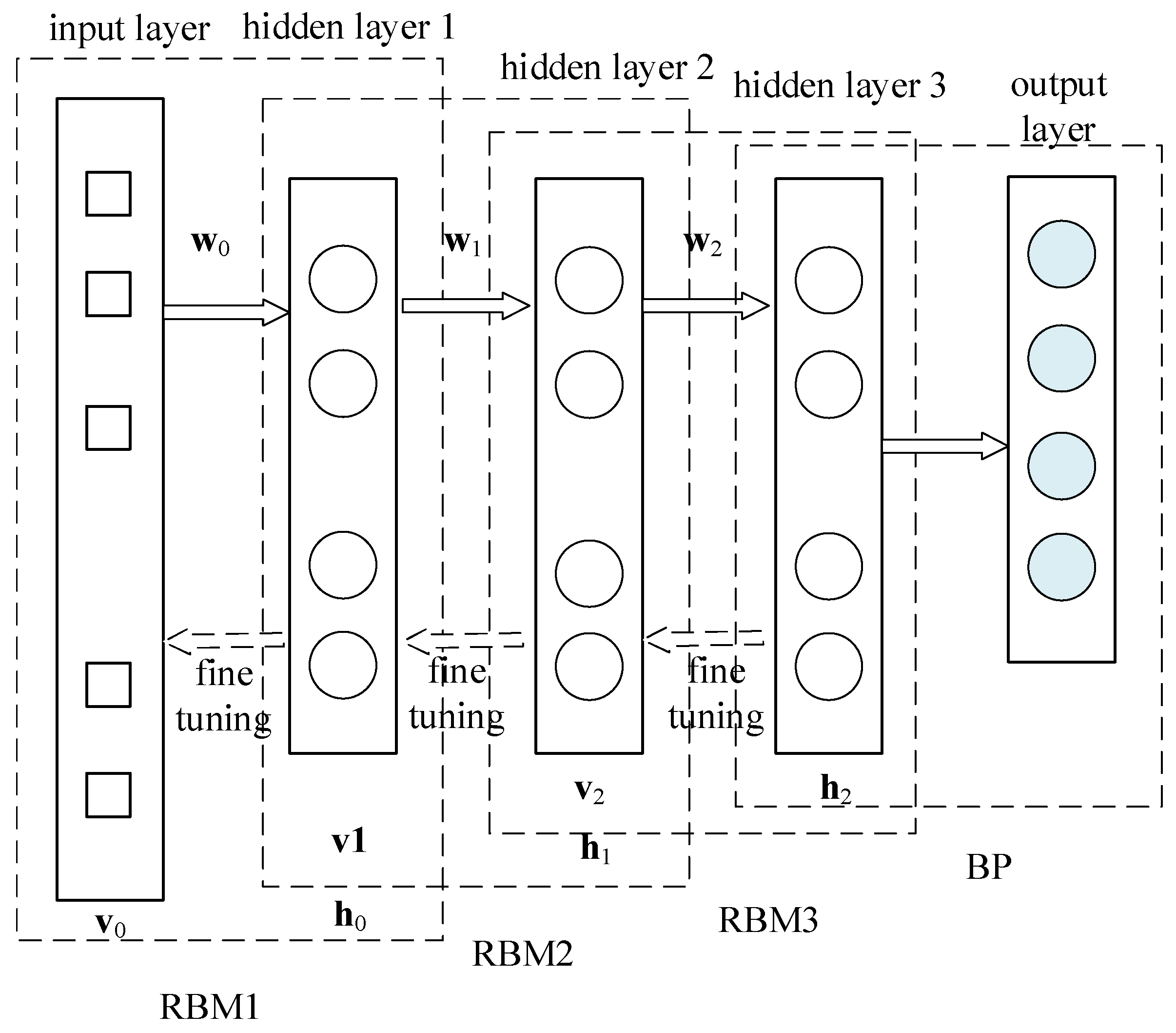
The DBN network structure comprises multiple layers of RBM and a Back Propagation (BP) network layer, as depicted in
Figure 2. Multiple layers of RBM are arranged in a stacked formation, with the initial layer serving as the input. the first hidden layer is used as the input and visible layer of the second hidden layer, and the second hidden layer forms the second RBM. This process is iterated until the final hidden layer and the output layer merge to create a functioning Backpropagation Network.
The DBN training process involves two steps: unsupervised layer-by-layer pre-training and supervised fine-tuning. Please refer to
Figure 2 for an overview of the training process.
The initial phase of unsupervised pre-training, carried out on a layer-by-layer basis, distinguishes DBN from other neural network models. By directly mapping the data from inputs to outputs, unsupervised layer-by-layer learning can acquire nonlinear complex functions, rendering the discrete-point fitting capacity of DBN highly potent. Unsupervised pre-training begins by taking the input feature data and the first hidden layer as RBM1. The input feature data values are then passed to the hidden layer through the RBM network, which subsequently reconstructs the visible layer with the hidden layer. Updating the weights between the hidden and visible layers according to the the difference between the reconstructed layer and visible layer. This process is repeated until the maximum number of iterations is reached, and the parameters of this RBM are trained, including the connection between the input layer v0 and the first hidden layer h0 weights w0, and the bias of each neuron in the input layer v0 and the first hidden layer h0. Then fix the network parameters of RBM1. Regard h0 as visible layer v1 and h1 as the new hidden layer. Form v1 and h1 into RBM2 for training and obtain its network parameters. Follow the same process to train RBM1, RBM2, and RBM3 to acquire their network parameters.
The next stage involves reverse fine-tuning, in which DBN establishes a BP network in the final layer to collect output data from RBMs and use it as input data to supervise the training of the BP network. The reverse network utilizes the BP network as a groundwork and transfers error information in the reverse direction to each layer of RBM. This fine-tunes the network parameters of all the RBMs in the entire network, ultimately minimizing the error value of the entire network.
2.3. DBN network structure and training
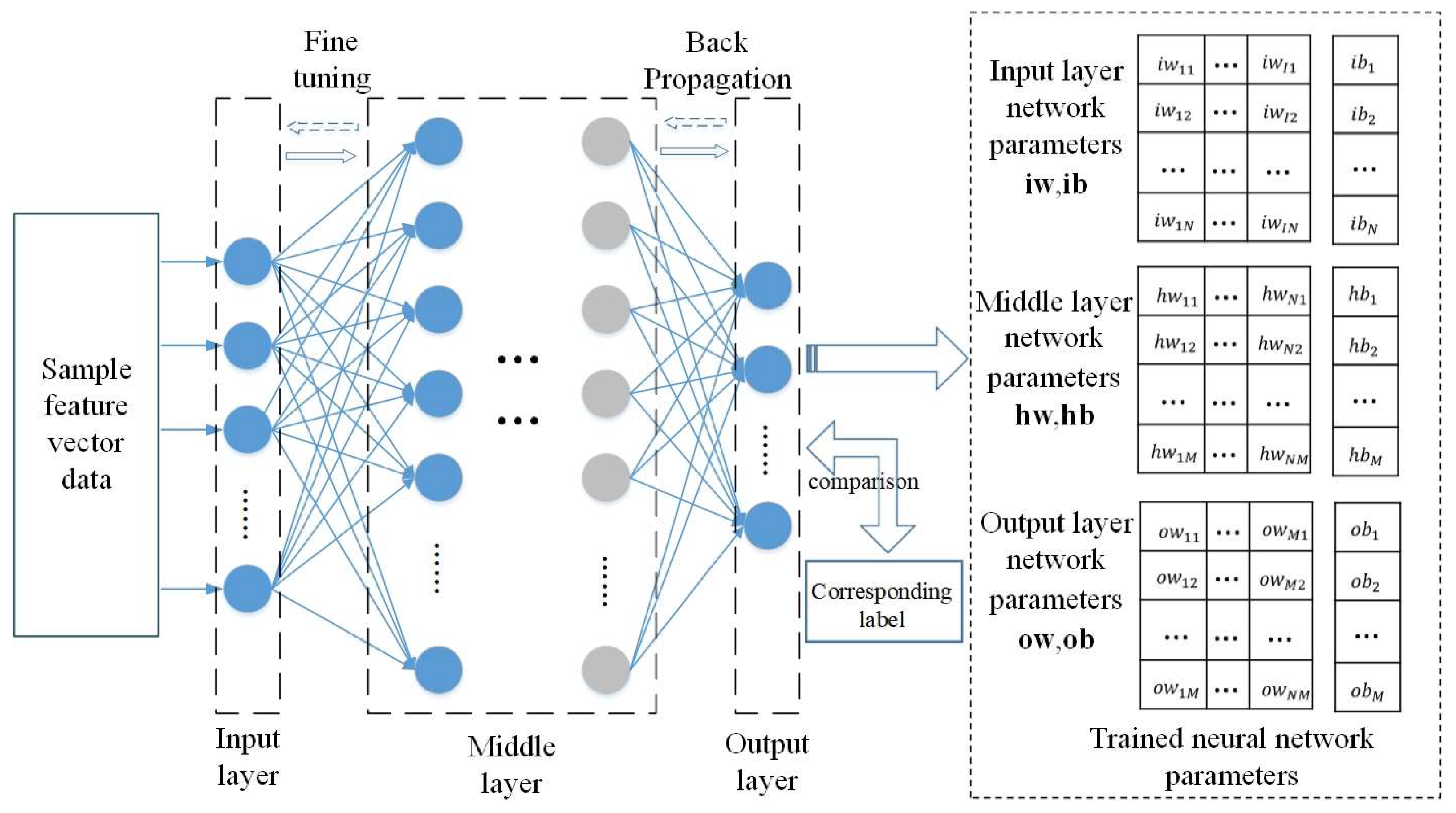
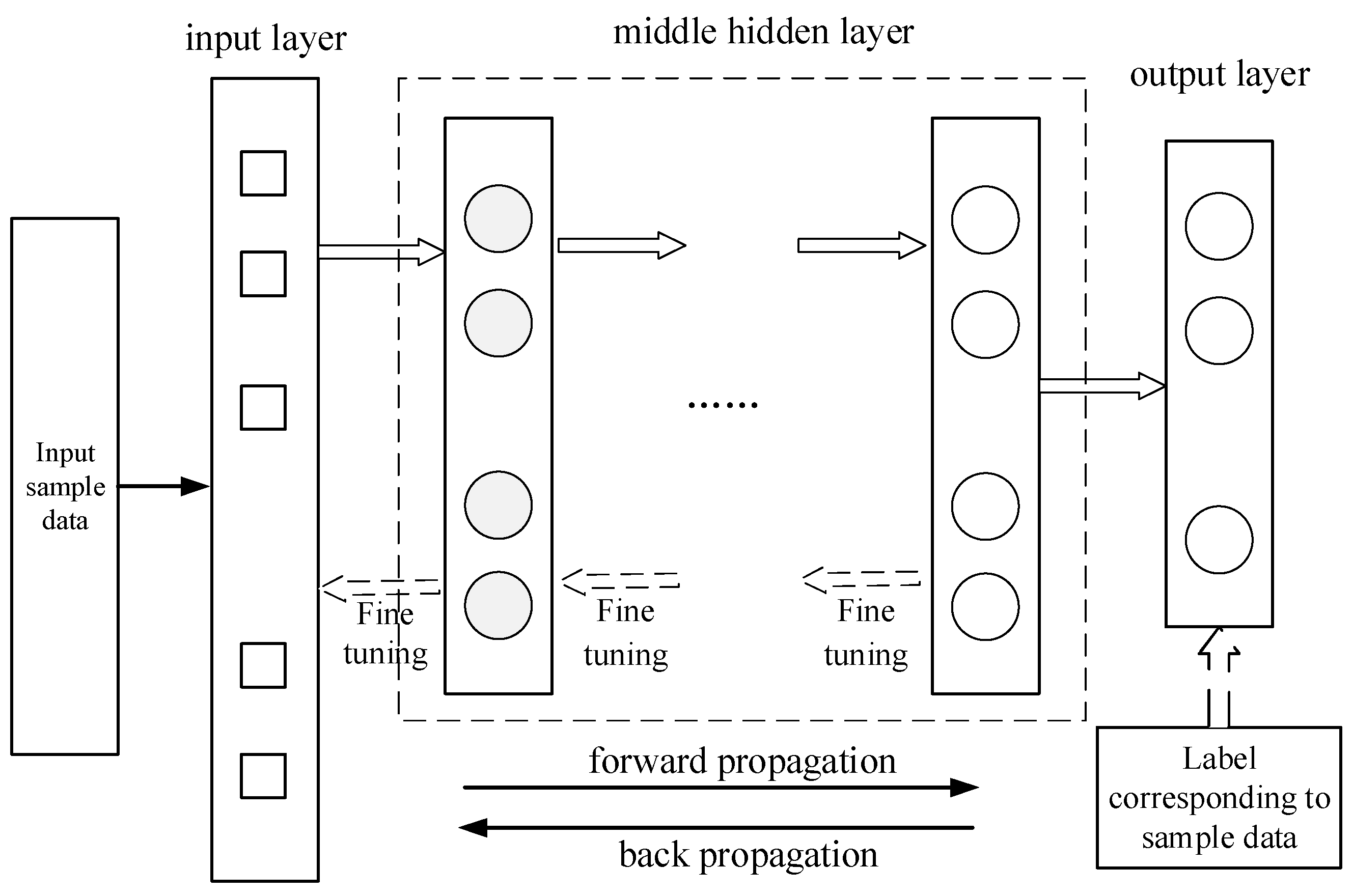
DBN classifiers can be trained base on DBN networks, as demonstrated in
Figure 3 of a DBN classifier, the sample feature data is used as input and the corresponding sample label serves as the output layer comparison standard for supervised DBN training. The relevant parameters of the DBN are fine-tuned using the commonly used back propagation algorithm in BP networks, resulting in the acquisition of the network and its parameters as a DBN classifier. Supervised training of the DBN can significantly decrease the training error and enhance the accuracy of the DBN classification model. In contrast to unsupervised training, where only one layer is trained at a time, backpropagation supervised fine-tuning updates the parameters of all layers simultaneously. Furthermore, the number of hidden layers in the DBN network can be modified according to specific requirements, with less or more than the 3 layers illustrated in the figure.
3. Multi-DBN weighted voting algorithm
Using multiple classifiers to vote can effectively improve the accuracy of classification, and the multiple DBN weighted voting method is described in detail below.
3.1. Method of voting
Voting, or Majority Voting[
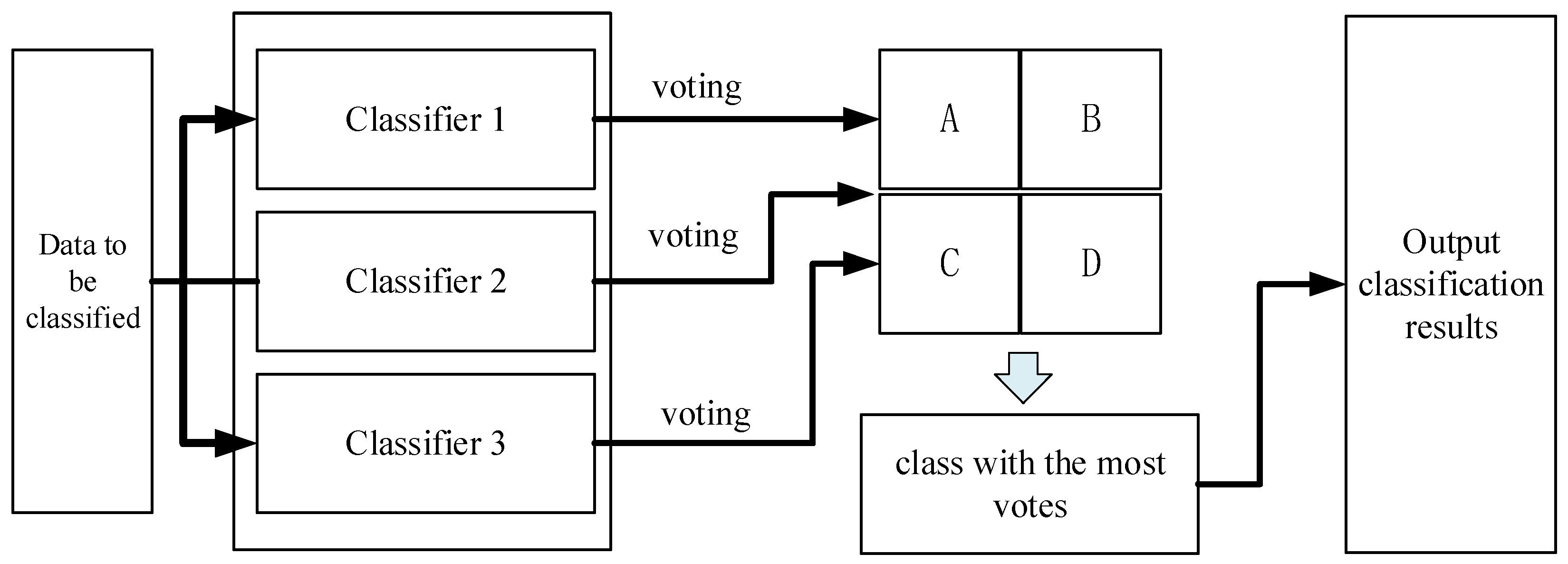
24], is a commonly employed method for combining classifiers. This method is based on the following principle: a set of trained base classifiers (Base Classifier) is used to make classification decisions on the feature data to be classified. Each base classifier casts a vote for the decision result that corresponds to the target class, and the class with the most votes is selected as the classification result for the entire set of classifiers. In this paper, three classifiers are utilized to determine the classification results through a voting process. Please refer to
Figure 4 for an illustration of the classification process.
Assume that there are
L base classifiers
Cl (l=1, 2, ...,
L) in the combined classifier, and the output of the each base classifier
Cl is a class probability estimate
P(
f(
w)
=k|Cl ), which represents the magnitude of the probability that the feature data to be classified,
w, is predicted as class
k (
k=1, 2, ...,) by the respective classifier
Cl . The probability estimates of all base classifiers are combined to calculate the following equation's value:
The combined classifier determines the probability that the feature vector,
w, belongs to class
k, and assigns w to the class with the highest probability value. If all classifiers within the combined classifier classify the feature vector
w to be classified as an independent event, the classification accuracy of the base classifiers after voting is raised to the P(
w), where each base classifier
Cl in the combined classifier has a classification accuracy of
Pc.
The function floor(.) rounds downward, while floor(L/2) represents the greatest integer not exceeding L/2. Take L=3 as an example to illustrate the classification accuracy of the combination classifier, the classification accuracy of the combination classifier is:
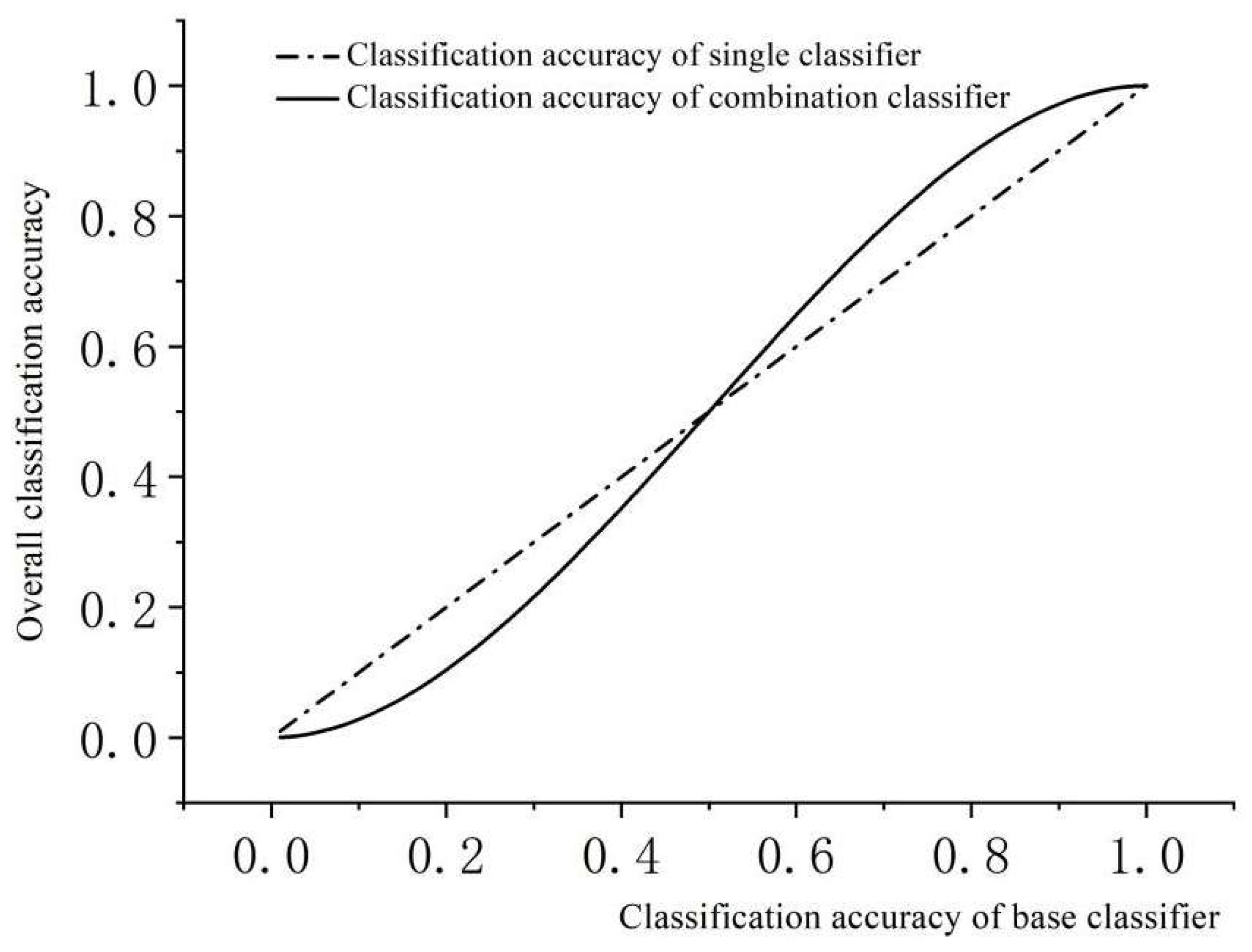
The classification accuracy P(w) is calculated with Pc as the variable, and figure 5.7 displays the trends of classification accuracy obtained using a base classifier with 1 and 3 classifiers, respectively.
Figure 5.
Trend of Combined Classifier Classification Accuracy.
Figure 5.
Trend of Combined Classifier Classification Accuracy.
When base classifiers accurately classify feature vectors over 50%, the accuracy of a combined classifier that utilizes three base classifiers to classify feature vectors through voting is significantly greater than that of a single classifier. The increased voting that takes place after classification by multiple classifiers allows for effective comparison of misclassified feature vectors of individual classifiers and subsequent correction of errors through the application of the "majority rule" principle.
The classification results using the voting algorithm in the best-case scenario without assigning weights to each classifier vote are displayed in
Table 1
When processing the voting results, the category with the most votes is identified as A, and the corresponding target category for the feature data then was classified as A. However, when the classifier is not set with the voting weights, voting classification using the voting method may result in target categories receiving the same number of votes, leading to an inability to classify them.
Table 2 displays an example of such voting results.
As shown in
Table 2, the tallied votes reflect an equal number of votes for the three categories: A, B and D. Consequently, it is unfeasible to determine the category corresponds to the given feature data with the highest votes. To address this predicament, we proposing voting weight values after achieved the classification results from each classifier.If the classification result of a classifier is considered to be more credible, it is given a larger voting weight, whereas a less credible result will be given a smaller weight. Even when multiple classifiers have voting results as displayed in Table 5.2, the final vote counts for each class will differ once weights are implemented. The class of the data to be classified can still be successfully determined.
3.2. Calculation of classifier weights
The primary challenge regarding the incorporation of voting weights is to establish the level of confidence in the classifier's classification results. To classify the target data, the DBN network is first trained using sample dataset and then implemented to classify the feature data of the target. The accuracy of classification depends on the performance of the DBN classifier that has been trained and the features of the data being classified. The features of the data cannot be controlled, and the classifier's performance is significantly influenced by the training sample dataset that was used. The principle of classifying neural networks assumes a functional relationship between target feature data and corresponding categories. Sample dataset is used to train the network so that it fits this relationship, processing the feature data for classification. Therefore, the degree to which the neural network accurately fits the function relationship of the entire network with the genuine mapping relationship between the target feature data and the corresponding category is highly dependent on the sample dataset used for training. The accuracy of the mapping relationship between the feature data fitted by the network and the corresponding class is greater when there is a large distance between target feature data of different classes and no data mixing occurs in the sample dataset. The Lance-Williams method[
25] is used to calculate the distance between sample data for training the classifier. The distance is calculated as follows:
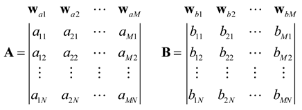
A, B, C, and D represent the sample data of four different vehicle signals detected by the WSN monitoring system. The feature matrices, which can also be regarded as a set of observations of the feature vectors, are shown in matrices A and B in equation (14). These matrices are obtained through feature extraction method applied to the sample data of these targets.The vector
wai denotes the
ith column observation of the feature matrix corresponding to the
A target signal, and
wbi denotes the
ith column observation of the feature vector corresponding to the
B target signal.
As demonstrated by the above equation, the characteristics A and B of the signal features for both kinds of targets are N × M matrices. N, which is the number of rows in the matrix, represents the number of segments into which the target signals that correspond to feature A are divided. M represents the number of variables in the feature vectors that are extracted from each signal sequence segment, which is twice the number of wavelet decomposition layers in thefeature extraction method. Columns in the matrix correspond to the feature vectors of the target signal in different dimensions. Hence, while computing the distance between two feature matrices, the first step is to calculate the distance between the eigenvectors of the same column of both feature matrices using equation (15).
Where
aij represents the
jth variable in the
ith eigenvector of the feature matrix
A and
bij is the
jth variable in the
ith eigenvector of the feature matrix
B. The feature matrix of the target signal contains M eigenvectors (
w1 , ... ,
wM ), after calculating the distance between the feature vectors in the feature matrix, quantization of the distance between the feature matrices and the target signal sequences is necessary.Equation (16) is utilized to calculate the distance between the matrices.
Where aij represents the jth variable in the ith eigenvector of the feature matrix A and bij is the jth variable in the ith eigenvector of the feature matrix B. The feature matrix of the target signal contains M eigenvectors (w1 , ... , wM ), after calculating the distance between the feature vectors in the feature matrix, quantization of the distance between the feature matrices and the target signal sequences is necessary.Equation (16) is utilized to calculate the distance between the matrices.
In the cross-voting classification method, merging multiple target sample data is required to train a classifier. Consequently, it is essential to compute the distance between merged matrices of multiple target signal feature matrices, utilizing the distances between single-target signal feature matrices. We apply the Lance-Williams formula for phase dissimilarity in a recursive manner to determine the distance between a solitary target dataset A and a combined set of multi-class target signal characteristics (
B ∪
C):
Equation (5.19) can be used for further derivation, yielding the distance between the merged dataset (
A ∪
D) and the merged dataset (
B ∪
C):
where
αA,D etc. is the adjustment factor, calculated through equation (5.20).
where
NB represents the number of rows in the feature matrix of class B signals and
NC represents the number of rows in the feature matrix of class C signals, which refers to the number of segments of the class C target signal during feature extraction.
The classification accuracy of a classifier is positively correlated with the spacing of the sample data used to train the classifier; the larger the spacing between the sample feature data of the target, the higher the average classification accuracy of the trained classifier; the smaller the distance, the lower the average classification accuracy. In view of the relationship between the training dataset and the performance of the classifiers, the multi-DBN voting classification method uses the spacing of the training sample data used by different classifiers to determine the voting weights of the classification results of the classifiers when using the voting method to integrate the results of different classifiers. When the training dataset spacing is larger, the trained binary classifiers have higher classification confidence and are assigned larger weights to their results; when the training dataset spacing is smaller, the corresponding classifiers are assigned smaller weights to their classification results.
Classifier weights are calculated from the sample feature data distance, which is used to map the distance between sample data to the voting weights domain of [0.7,1.3].This range was chosen due to its optimal performance in previous studies. The voting weights domain guarantees that the combined weights of the two classifier results are greater than the largest classifier result weight. The combined set spacing of the sample data for the training of the three classifiers in the weighted voting method is respectively
Dist(1),
Dist(2),
Dist(3), we use the following formula to calculate the weights of each classifier result when voting:
where
NorD(
i) represents the normalized distance between the merged sets of sample data,
P(
i) is the voting weight of the result of the
ith classifier. To ensure that the value of the classifier result voting weight
P(
i) is in the range of [0.7, 1.3], the absolute value of the distance between the normalized merged sets denoted as
|NorD(
i)| must provide a value within the range of [0.2, 0.8]. Since the value range of
is [-1, 0], an adjustment coefficient,
δ, is required to ensure that |NorD(i)| meets the condition. The acceptable range for
δ is between 0.2 and 0.8, and we have chosen to set to 0.3.
4. Engineering implementation of the algorithm
Neural networks require significant computation during training, but the microcontroller processor chips utilized in WSN intelligent monitoring system nodes lack the capability to handle this task. To address this issue, the multi-DBN voting classification method necessitates the implementation by adopting "top-end training and bottom-end transplantation" approach.This approach entails training the DBN network on a PC and transplanting its network parameters to the WSN nodes during project implementation. The DBN network is trained on the computer side, and network parameters are then transferred to the WSN nodes. Finally, the features to be classified are calculated and voted on to determine the final classification results.
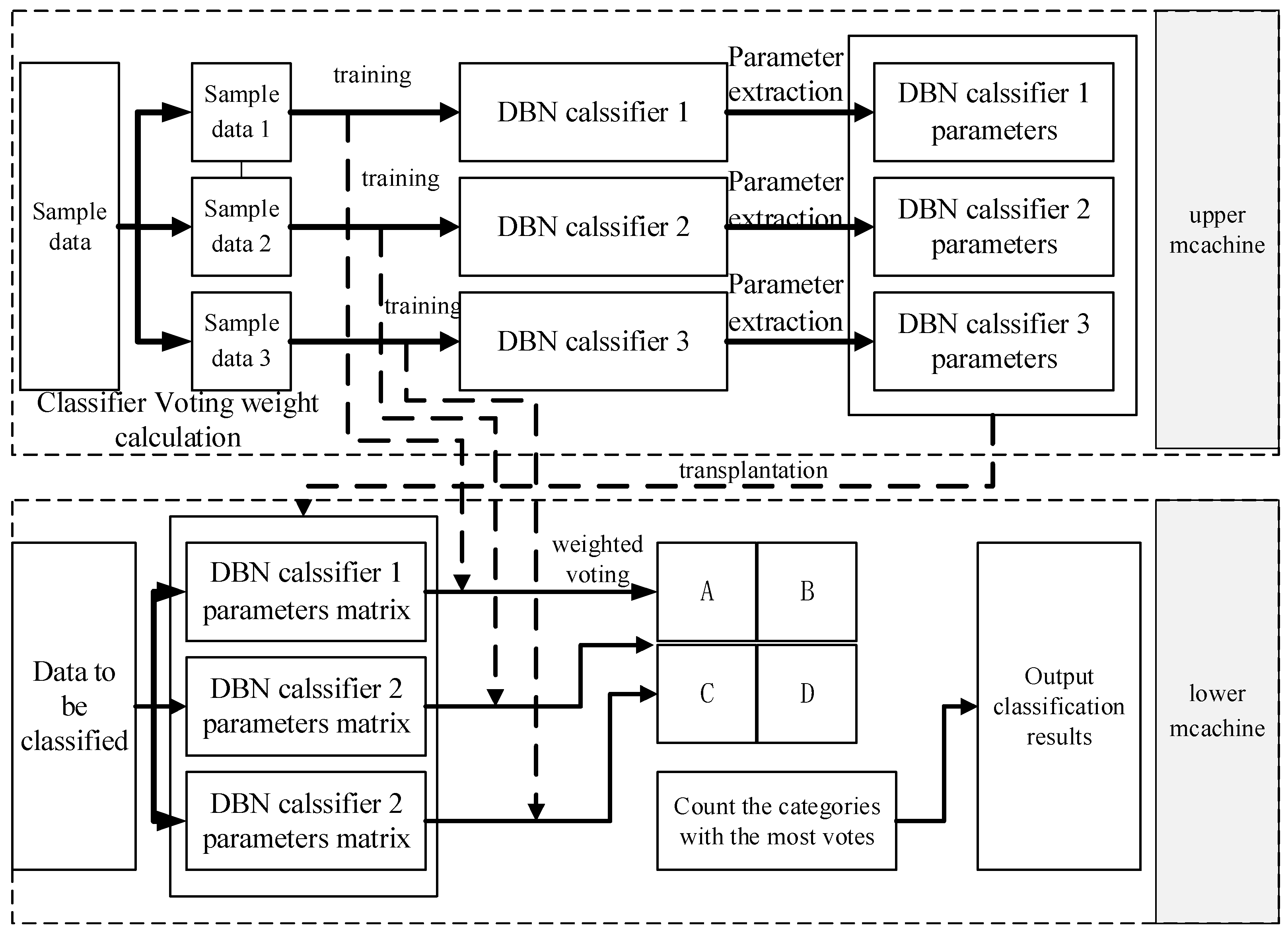
The algorithm's process is illustrated in
Figure 5.9. Initially, the PC carries out "top-end training" processing. This training involves using segmented feature data samples to train multiple DBN classifiers. Additionally, the voting weights of the classifiers to be identified along with the sample data of the segment are calculated while obtaining the network parameters of several DBN classifiers at the end of the training. After completing the training, the parameters of multiple DBN classifiers are acquired, which includes the connection weights between the multi-layer neurons and the neuron bias. Following that, "down-end transplantation" is performed on the WSNnode. The network parameters of multiple DBN classifiers are exported and stored in the memory chip of the processor unit of the WSN intelligent monitoring system. Lastly, the feature data that requires classification is processed by operating it with the parameters of multiple DBN networks to obtain the classification results of multiple classifiers. The results of multiple classifiers are utilized to conduct weighted voting classification. Firstly, classification results of multiple classifiers obtained from the operation are used in weighted voting. Then, respective vote scores of categories A, B, C, and D are calculated, and the one with the highest vote score is taken as the final classification result.
Figure 6.
Flow ot the Multi-DBN Vote Classification Algorithm.
Figure 6.
Flow ot the Multi-DBN Vote Classification Algorithm.
The following sections provide explanations for the training of the neural network, transplantation of the network, segmentation of training data, and calculation of corresponding voting weights.
4.1. Training of Neural Networks
Figure 7.
Flow of "Upper Training" in Multi-DBN Vote Classification Algorithm.
Figure 7.
Flow of "Upper Training" in Multi-DBN Vote Classification Algorithm.
Neural networks can be computationally demanding and time-consuming during training, particularly when used in lower-performance embedded processor units. To address this challenge, a common strategy is to train the network on the PC and then transplante it to the embedded processor unit for use.
The top-training phase of the multi-DBN weighted voting classification algorithm, which involves training and transplanting the DBN network, is illustrated in
Figure 5.10. Here, the DBN network is initially trained utilizing sample feature data, and the parameters of the DBN classifiers are obtained following the completion of the training.
When training a DBN network, predetermined values should be set for the number of layers and number of neurons in each layer. The number of neurons in the input and output layers depends on the sample feature data and the number of target categories. The feature vectors extracted in this study are 16-dimensional, thus requiring 16 neurons in the input layer to correspond to each value. The output layer consists of four neurons corresponding to the four target categories (A, B, C, and D). For the four target categories, A, B, C, and D are assigned the values of (1 0 0 0), (0 1 0 0), (0 0 1 0), and (0 0 0 1) respectively. This allows for the output of 1 to correspond to a neuron in the output layer for each category. The network requires a pre-set number of intermediate layers and neurons in each layer. For this paper, we have set 2 intermediate layers with 100 and 60 neurons per layer, respectively.
For details on the training methods and specific processes of the DBN network, please refer to the literature[
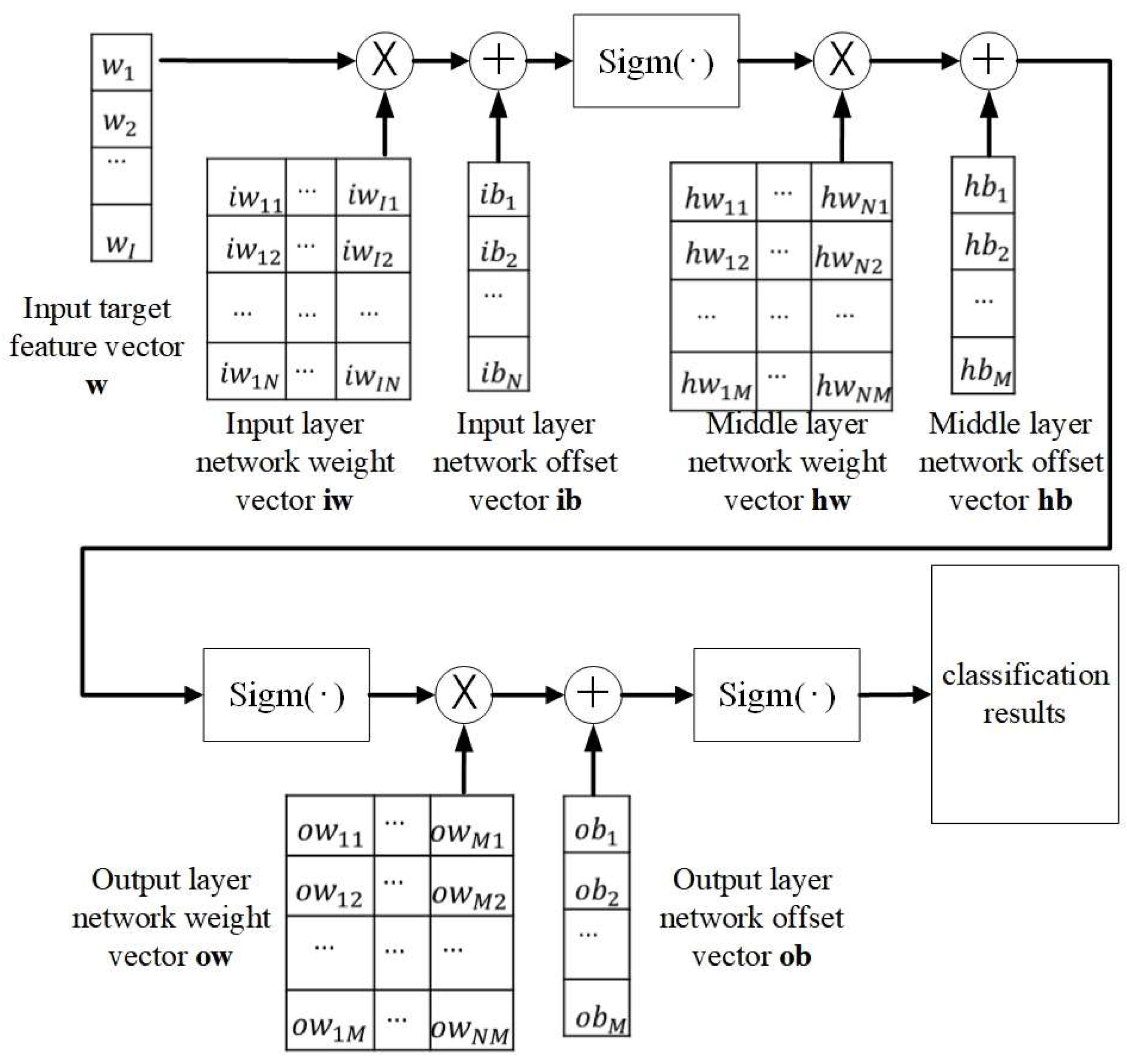
26]. The trained DBN network can be represented by a set of parameters, including the input layer network weight matrix
iw, input layer neuron bias vector
ib, intermediate layer network weight matrix
hw, intermediate layer neuron bias vector
hb, output layer network weight matrix
ow, and the output layer bias vector
ob.
4.2. Transplanting of DBN Classifier
After training the DBN, a set of network parameters are settled, which are also the parameters of the trained classifier. These network parameters are exported and deposited into the processor unit on the node of the WSN intelligent monitoring system to classify the data according to this set of parameters.
Figure 8.
Calculation process using DBN classifier network parameters for classification.
Figure 8.
Calculation process using DBN classifier network parameters for classification.
The computational flow for classifying the target data using the trained network parameters is illustrated in
Figure 5.11. The feature vector utilized for classification is represented by the symbol
w. The equation for determining the classification result, denoted as
r, is displayed in Eq.(20).
Where sigm(.) is the selected sigmoid activation function for training, the formula displayed below:
4.3. Classifier training data preprocessing
When training the DBN classifiers with sample data, some training data with large deviations from the mean value may cause misclassification by the trained classifiers, leading to poorer algorithm performance. Moreover, using the same training dataset to train all three classifiers does not fully optimize the performance of the comparison segment of the algorithm, which is a characteristic of the voting method. Thus, the training data is processed using the segmented averaging means to ensure that the dataset for training the three classifiers has a certain degree of variation to minimize the impact of outliers on the classifiers' classification performance.
Assuming the sample data is a feature matrix F with N feature vectors as depicted below:
The feature matrix is initially partitioned into three sections, namely
FP1,
FP2, and
FP3, as illustrated in the equation below:
To minimize the impact of outlying values in the training data on the classifier's performance, we perform an averaging treatment on the three data segments. The first segment remains unchanged, the first and second segments' data are averaged to create the new second segment data, and the first, second, and third segments' data are averaged to create the new third segment data. The resulting averaged segment data,
FT1,
FT2 and
FT3, are listed below.
The main purpose of segmenting the feature matrix of the sample data is to create a varied training dataset for the three DBN classifiers. This results in different network parameters for each trained DBN classifier, allowing the algorithms to effectively compare and vote. Additionally, averaging the segmented data aims to eliminate outliers in the training data.
5. Performance of multi-DBN weighted voting algorithm
In this paper, the proposed algorithm is validated using the feature data of four targets, which are AAV vehicles, DW vehicles, small domestic vehicles, and pedestrians. Among them, the signal data of AAV vehicles, DW vehicles from are gathered from a real-world experiment, named the third SensIT situational experiment[
27]. In the experiment, 75 sensor nodes with acoustic, seismic, and infrared sensing capability were located at the Marine Corps Air Ground Combat Center. Testing runs were performed by driving different kinds of vehicles across the testing field. Four target vehicle classes, namely assault amphibian vehicle (AAV), main battle tank, high-mobility multipurpose wheeled vehicle, and dragon wagon (DW) were used. The acoustic and seismic data of each run were recorded and the sampling rate of the signals was 4096 Hz. There were three different paths in the experimental area for the vehicles to pass, and a testing run was accomplished by driving the vehicle on the path. A series of numbers was utilized to indicate these runs, i.e., DW3, DW4, DW5. The acoustic and seismic data of each run were recorded by the sensor nodes deployed at the side of the road. The details of the experiment were described in the paper mentioned above.
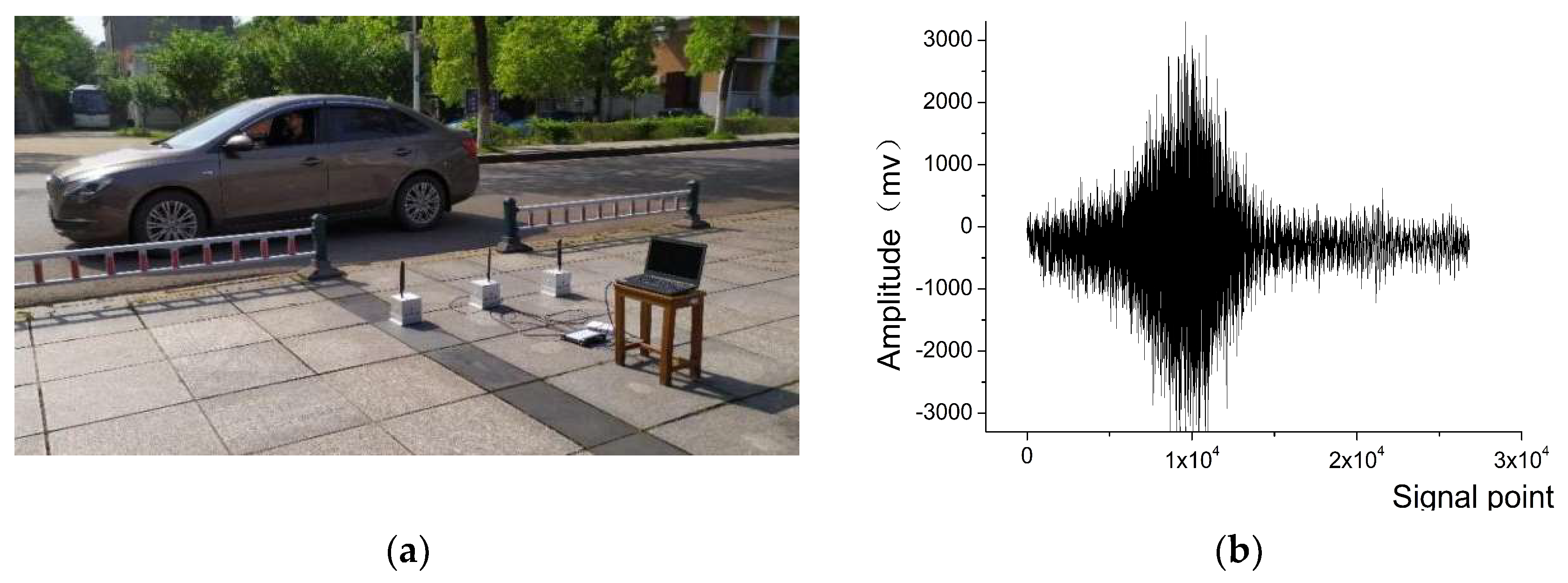
The signal of small vehicle and personnel were tested in real-world scenarios using WSN nodes specialized for collecting signals. The sensor nodes were placed on open ground at various distances from the road, with adjustments made gradually. WSN nodes collected sound, vibration, infrared, and magnetic signals from a range of targets including various types of vehicles and individuals. The experiment selects the acoustic and vibration signals obtained from small vehicles and personnel targets. The schematic diagram demonstrating the experiment is presented in
Figure 9(a), and
Figure 9(b) shows the acquired acoustic signals of small vehicle.
The data from both AAV and DW vehicles in the SensIT dataset, as well as from personnel and small vehicles in the acquired dataset show above, are combined to create a multi-target signal dataset for the validation of the multi-DBN voting classification algorithm.
5.1. Performance Analysis of Multi-DBN Weighted Voting Algorithm
The SensIT experiment employed AAV vehicles and DW vehicles, while the introduced experiment in
Figure 9 utilized personnel and small vehicles as the four target to be classified. Using selected acoustic signals from the acoustic datasets of four target types (AAV3, AAV4, DW3, and DW4 datasets in SensIT), along with the personnel and vehicle data from the first two experiments in the acquired datasets, and corresponding seismic signal data from the seismic datasets of the aforementioned targets (AAV3, AAV4, DW3, and DW4 dataset in SensIT). Extract acoustic-seismic mixed features of the sample data using the WCER feature extraction algorithm[
16]. The target category label corresponding to the AAV vehicle target feature data is set to be {1 0 0 0}; the target category label corresponding to the DW vehicle sample feature data is set to be {0 1 0 0}; the target category label corresponding to the personnel target feature data is set to be {0 0 1 0}; and the target category label corresponding to the small vehicle target feature data is set to be {0 0 0 1}.
Three DBN classifiers were used for vote classification, each with the same network size, containing one input layer, two intermediate hidden layers and one output layer. The input layer of the classifier network contains 16 neurons, representing the 16-dimensional feature vectors of the WSN monitoring system targets. The first hidden layer of the intermediate layer contains 100 neurons, and the second hidden layer contains 60 neurons. The output layer contains 4 neurons, corresponding to the 4 different types of targets.
The sample target feature data is first segmented and averaged, which was then divided into three equal-sized segments, for training three DBN classifiers. The voting weights for these classifiers are then calculated using the aforementioned sample feature data segments. The three trained classifiers are fed the feature data for calculation and voting classification. The resulting classification is then compared to the original target categories to determine accuracy. After obtaining accuracy for all datasets, the average classification accuracy for each target category is calculated.
According to
Table 3, The following conclusions can be drawn from the results of the multi-DBN voting classification method for classifying AAV vehicles, DW vehicles, personnel, and small vehicles.
The proposed multi-DBN classification algorithm can accurately classify various targets in the WSN monitoring system, with a classification accuracy of over 70% for the four target categories in the validation test dataset. (2) The multi-DBN weighted voting classification algorithm enhances the overall classification accuracy when compared to the average results of the three individual classifiers for AAV targets. The voting session significantly improves accuracy rates by about 5% when compared to the single DBN classification. The classification accuracy rate for DW targets increased by approximately 5.86%, while the rate for personnel targets increased by 6%. Additionally, the multi-DBN weighted voting classification algorithm is a weighted algorithm that utilizes multiple-DBNs. The increase in classification accuracy is approximately 6.5%. For targets of small vehicles, the increase in classification accuracy is approximately 3.49%. (3)Additionally, the classifiers' performance varies based on the sample data used to train them. For AAV targets, the classification accuracy of classifiers trained using the third segment of sample data after segmentation is significantly lower compared to the first two classifiers.(4) The classification accuracy of classifiers for both AAV and DW targets is generally low, which can be attributed to their lower accuracy for both target types. Classification accuracy is generally low because the acoustic and vibration Seismic of AAV targets and DW targets are similar, and it is more difficult to distinguish the feature data after WCER feature extraction.
5.3. Effect of DBN network size on algorithm classification accuracy
The DBN classifiers' network parameters differ depending on the sample data they are trained with.
Table 3 illustrates that when comparing DBN classifiers with different parameters, they do not show the same classification accuracy for the identical feature data under classification. To study how different network sizes affect the classification accuracy of DBN classifiers and multi-DBN voting classification algorithms, we constructed various sizes of DBN classifiers and trained them with identical sample feature data outlined in the preceding section. Afterwards, we classified the remaining dataset and calculated comparative classification accuracies.
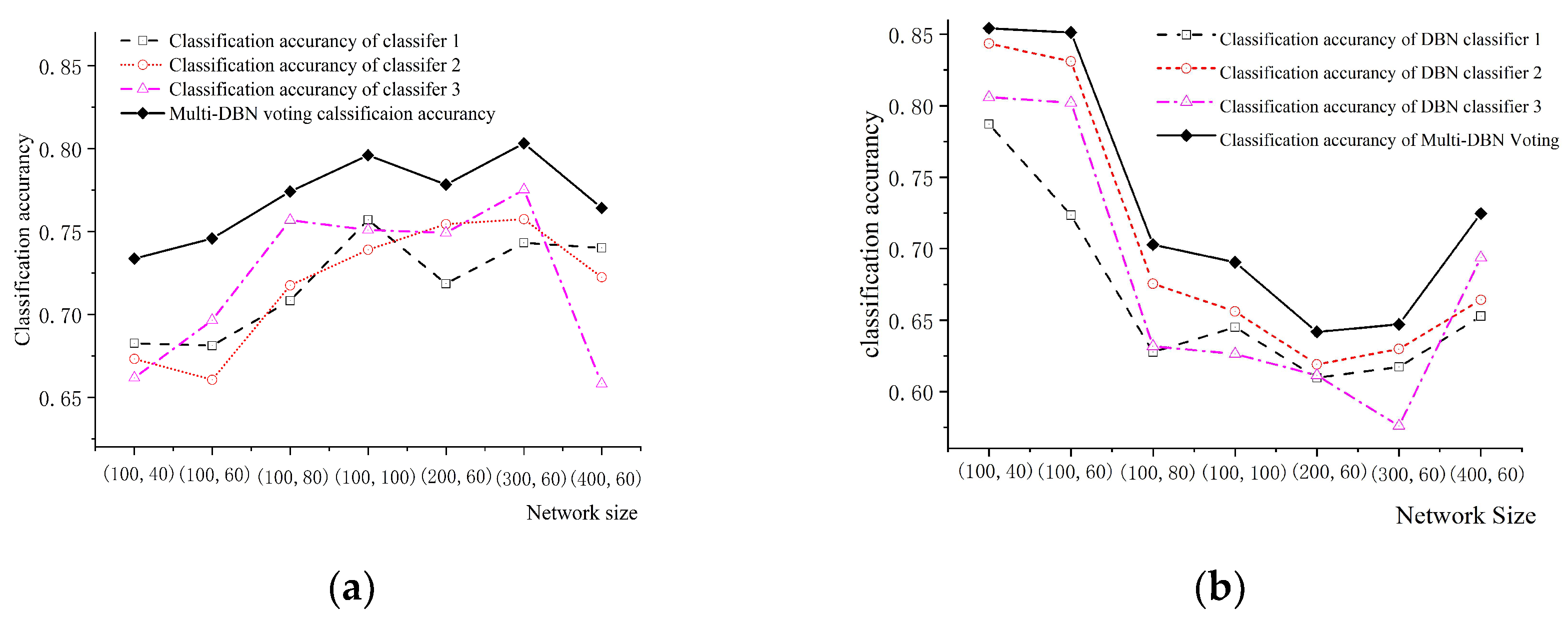
Respectively, the following scaled networks were constructed for three DBN classifiers: (1)The first hidden layer of the intermediate layer contained 100 neurons, and the second hidden layer contained 40 neurons; (2)The first hidden layer of the intermediate layer contained 100 neurons, and the second hidden layer contained 60 neurons; (3)The first hidden layer of the intermediate layer contained 100 neurons, and the second hidden layer contained 80 neurons; (4)The first hidden layer of the intermediate level contained 200 neurons, and the second hidden layer had 60 neurons; (5)The first hidden layer of the middle level consisted of 300 neurons, and the second hidden layer had 60. The classification accuracy of three DBN classifiers and multi-DBN voting classifiers were computed. The classification results for both AAV vehicles and DW vehicles are illustrated in
Figure 10.
From the figure displaying the classification accuracies of the single classifier and the multi-DBN voting method at various network sizes, it is evident that the multi-DBN voting classification algorithm exhibits higher accuracy than the highest accuracy of the three DBN classifiers. Additionally, there is no discernable correlation between network size and classification accuracy, and larger networks do not necessarily result in higher accuracy. As illustrated in
Figure 10, the accuracy of classifying DW vehicles declines as the network size increases. Large-scale neural networks tend to overfit more than their smaller counterparts. Additionally, the DBN classifier's classification accuracy for AAV vehicles is negatively correlated with that for DW vehicles when classifying multiple targets. When the classifier's accuracy for AAV vehicles improves, the corresponding accuracy for DW vehicles decrease.
There is no direct relationship between the size of the network and classification accuracy in the classification of multi-targets using either the multi-DBN voting classification algorithm or a single DBN classifier. Therefore, it is important to comprehensively consider the actual application scenario of the method to select the appropriate network size. As network size increases, "down-end transplantation" requires more memory and computation source.
5.4. Comparison with other multi-objective classification methods
In addition to deep learning algorithms, Forward Feedback Neural Network (FFNN) [
28], the Plain Bayes (NB) method[
29], adaboosting [
30], and the Extreme Learning Machine (ELM) [
31] algorithms are also well-established classical methods for multi-classification. These centralized methods were applied to classify the four target signals in the WSN monitoring system and compare the results with those of the multi-DBN voting methods.
Define the overall average classification accuracy
OAc,
OAc is calculated based on the average classification accuracy of a single class of targets, assuming that the classification accuracy of the ith class of targets is
Ac(
i) (
i = 1, 2, ... , P; P is the number of target categories in the dataset, which in this case is 4), then the overall average classification accuracy
OAc is calculated using Equation(25).
Table 4 shows the overall average classification accuracy of each classification algorithm for four kinds of targets.
Where the average classification time is determined by adding the classification time for all data records in the dataset and dividing by the total number of data records. Based on the overall average classification accuracy results of each algorithm for the four targets presented in the table, We can draw the following conclusions:
(1)The NB method yields a lower average classification accuracy of approximately 63.85% when used to classify multiple vehicle signals detected in the WSN system. The main reason for this is that when the sample training dataset is small, the a priori probability model obtained by analyzing the training data using the Naive Bayes (NB) method is not accurate.
(2)Additionally, when classifying multiple target signals using the Adaboosting method, the accuracy is lower compared to other methods.
(3)When classifying multiple vehicle signals detected in the WSN monitoring system, the neural network-related methods (such as the multi-DBN voting method and FFNN method) exhibit higher average classification accuracy. Moreover, the neural network method's advantage in classification accuracy becomes more apparent after the network optimization.
(4) The multi-DBN voting method achieves the highest classification accuracy, although its classification time is the longest compared to other methods.
When implementing the multi-DBN neural network using "top-end training, bottom-end transplantation" approach, the main memory consumption occurs during the top-end training phase. The memory consumption of bottom-end transplantation is dependent on network parameters. In this paper, we used a four-layer network for the DBN classifier with a total of 280 neurons, divided into 16, 100, 60, and 4 respectively. The resulting network parameters consist of six matrices, sized 16×100, 16×1, 100×40, 100×1, 40×4, and 40×1, respectively, occupying approximately 11.8 kB of memory space. With these modest requirements, our approach can be feasibly implemented on WSN nodes possessing limited computational and memory resources.
6. Conclusions
In this paper, a novel method for multi-target classification in WSNt monitoring systems,on the basis of single DBN classifier and combined with the idea of voting method, which named multi-DBN weighted voting classification method is proposed. The introduced appraoch using multiple DBN classifiers cooperating with each other to classify multi-targets. According to the training and classification characteristics of neural networks, we propose the strategy of "top-end training, bottom-end transplantation", and transplant the multi-DBN weighted voting classification method to the WSN node for engineering implementation. The experiment reveals that the multi-DBN weighted voting algorithm enhances the target classification accuracy by approximately 5% in comparison to the single DBN classifier,achieving an average classification accuracy of 84.63% across four different types of moving targets. Moreover, the increased memory requirement remains tolerable within thenode's limits in WSN.
Author Contributions
Conceptualization,H.Z.; Investigation,H.Z., and Y.Z.; Methodology,H.Z., L.F., G.B., P.C., S.L., and C.T.; Software, H.Z.; Supervision, H.Z., and Y.Z.; Writing—original draft, H.Z.; Writing—review and editing, H.Z., and Y.Z. All authors have read and agreed to the published version of the manuscript..
Funding
This research received no external funding.
Institutional Review Board Statement
Not applicable.
Informed Consent Statement
Data used in this work were not generated by the authors but obtainedfrom a publicly available dataset developed by Broderick, Michael P. et al. [
27].
Data Availability Statement
This work used data publicly available from [
27].
Conflicts of Interest
The authors declare no conflict of interest.
References
- Sohraby, K.; Minoli, D.; Znati, T. Wireless sensor networks: technology, protocols, and applications, 1st ed.; John Wiley & Sons, INc.: Hoboken, New Jersey, 2007.
- Mishra, D.P.; Dorale, S.S. An Application of Wireless Sensor Network in Intelligent Transportation System. 2013 6th International Conference on Emerging Trends in Engineering and Technology, Nagpur, India, 2013, pp.90-91.
- Balid, W.; Tafish, H.; Refai, H.H. Development of Portable Wireless Sensor Network System for Real-time Traffic Surveillance. 2015 IEEE 18th International Conference on Intelligent Transportation System, Spain, 2015, pp.1630-1637.
- Hsu, C.W.; Lin, C.J. A comparison of methods for multiclass support vector machines. IEEE Transactions on Neural Networks 2002. 13, 415-425. [CrossRef]
- Manikandan, J.; Venkataramani, B. Design of a Modified One-Against-All SVM Classifier, 2009 IEEE International Conference on Systems Man and Cybernetics, San Antonio, USA, 2009, 1869-1874. [CrossRef]
- Fei, B.; Liu, J.B. Binary tree of SVM: A new fast multiclass training and classification algorithm. IEEE Transaction on Neural Networks 2006. 17, 696-704. [CrossRef]
- Cheng, L.L.; Zhang, J.P.; Yang, J.; Ma, J. An Improved Hierarchical Multi-Class Support Vector Machine with Binary Tree Architecture. 2008 International Conference on Internet Computing in Science and Engineering, Proceedings, Harbin, China. 2008, 106-109.
- Wang, Y ; Cheng, XL ; Li, X ; Li, BQ ; Yuan, XB. Powerset Fusion Network for Target Classification in Unattended Ground Sensors. IEEE SENSORS JOURNAL 2021. 21. 12. [CrossRef]
- Xu, TH; Wang, N ; Xu, X. Seismic Target Recognition Based on Parallel Recurrent Neural Network for Unattended Ground Sensor Systems. IEEE ACCESS 2019. 7,137823-137834. [CrossRef]
- Belsare, K ; Singh, M; Gandam, A; Malik, PK; Agarwal, R; Gehlot, A. An integrated approach of IoT and WSN using wavelet transform and machine learning for the solid waste image classification in smart cities. TRANSACTIONS ON EMERGING TELECOMMUNICATIONS TECHNOLOGIES 2023.9. [CrossRef]
- Kim, Y; Jeong, S; Kim, D. A GMM-Based Target Classification Scheme for a Node in Wireless Sensor Networks. IEICE TRANSACTIONS ON COMMUNICATIONS 2008.11.3544-3551. [CrossRef]
- Zhao, Q ; Guo, F ; Zu, XS ; Chang, YC; Li, BQ ; Yuan, XB. An Acoustic Signal Enhancement Method Based on Independent Vector Analysis for Moving Target Classification in the Wild. SENSORS. 2017.12.17-10. [CrossRef]
- Xu, T.A. New Sphere-Structured Multi-Class Classifier, Proceedings of the 2009 Pacific-Asia Conference on Circuits, Communications and Systems 2009,520-525,Chengdu, People’s Republic of China. [CrossRef]
- Tomar, D.; Agarwal, S.A. Comparison on multi-class classification methods based on least squares twin support vector machine. Knowledge-based Systems 2015. 81, 131-147. [CrossRef]
- Mohamed, AR ; Dahl, GE ; Hinton, G. Acoustic Modeling Using Deep Belief Networks. IEEE TRANSACTIONS ON AUDIO SPEECH AND LANGUAGE PROCESSING. 2012.20-1. [CrossRef]
- Zhang, H ; Pan, ZM; Zhang, WN. Acoustic-Seismic Mixed Feature Extraction Based on Wavelet Transform for Vehicle Classification in Wireless Sensor Networks.2018.18-6. [CrossRef]
- Wang, GM; Qiao, JF ; Bi, J ; Jia, QS; Zhou, MC. An Adaptive Deep Belief Network With Sparse Restricted Boltzmann Machines. IEEE TRANSACTIONS ON NEURAL NETWORKS AND LEARNING SYSTEMS. 2020-31-10. 4217-4228. [CrossRef]
- Sarikaya, R; Hinton, GE ; Deoras, A. Application of Deep Belief Networks for Natural Language Understanding. IEEE-ACM TRANSACTIONS ON AUDIO SPEECH AND LANGUAGE PROCESSING. 2014. 22-4. [CrossRef]
- Ahmadian, S ; Khanteymoori, AR. Training back propagation neural networks using asexual reproduction optimization. 2015 7TH CONFERENCE ON INFORMATION AND KNOWLEDGE TECHNOLOGY (IKT). 2016.
- Mourgias-Alexandris, G ; Tsakyridis, A; Passalis, N ; Tefas, A ; Vyrsokinos, K; Pleros, N. An all-optical neuron with sigmoid activation function. OPTICS EXPRESS. 27-7. 9620-9630. [CrossRef]
- Ma, XS ; Wang, XJ. Average Contrastive Divergence for Training Restricted Boltzmann Machines. ENTROPY. 2016. 18-1. [CrossRef]
- Roussel, C; Cocco, S ; Monasson, R. Barriers and dynamical paths in alternating Gibbs sampling of restricted Boltzmann machines. PHYSICAL REVIEW E. 104-3. [CrossRef]
- Larochelle, H ; Mandel, M ; Pascanu, R ; Bengio, Y. Learning Algorithms for the Classification Restricted Boltzmann Machine. JOURNAL OF MACHINE LEARNING RESEARCH. 2012. 13.643-669.
- Huang, CH ; Wang, JF. Multi-weighted Majority Voting Algorithm on Support Vector Machine and Its Application. TENCON IEEE Region 10 Conference Proceedings. Singapore. 2009.
- Tang, Q; Xiao, JY ; Wu, KF. A novel evidence combination method based on stochastic approach for link- structure analysis algorithm and Lance- Williams distance. PEERJ COMPUTER SCIENCE. 2003. 9. [CrossRef]
- Zhou, SS ; Chen, QC ; Wang, XL . Fuzzy deep belief networks for semi-supervised sentiment classification. NEUROCOMPUTING. 131. 312-322. [CrossRef]
- Duarte, M.F.; Hu, Y.H. Vehicle classification in distributed sensor networks. J. Parallel Distrib. Comput. 2004, 64, 826–838. [CrossRef]
- Asadi, R; Kareem, SA. Review of Feed Forward Neural Network classification preprocessing techniques. PROCEEDINGS OF THE 3RD INTERNATIONAL CONFERENCE ON MATHEMATICAL SCIENCES. 1602. 567-573. [CrossRef]
- Zhang, ZH. Naive Bayes classification in R. ANNALS OF TRANSLATIONAL MEDICINE. 2016. 4-12. [CrossRef]
- Chao, W ; Bo, L; Lei, W ; Pai, P . Improving boosting methods with a stable loss function handling outliers. INTERNATIONAL JOURNAL OF MACHINE LEARNING AND CYBERNETICS. 14-7. 2333-2352. [CrossRef]
- Cao, JW ; Lin, ZP ; Huang, GB ; Liu, N. Voting based extreme learning machine. INFORMATION SCIENCES. 2012. 185-1. [CrossRef]
|
Disclaimer/Publisher’s Note: The statements, opinions and data contained in all publications are solely those of the individual author(s) and contributor(s) and not of MDPI and/or the editor(s). MDPI and/or the editor(s) disclaim responsibility for any injury to people or property resulting from any ideas, methods, instructions or products referred to in the content. |
© 2023 by the authors. Licensee MDPI, Basel, Switzerland. This article is an open access article distributed under the terms and conditions of the Creative Commons Attribution (CC BY) license (http://creativecommons.org/licenses/by/4.0/).
