Submitted:
27 October 2023
Posted:
27 October 2023
You are already at the latest version
Abstract
In this study, we introduce the dynamics of a Hepatitis B virus (HBV) model with the class of asymptomatic carriers and conduct a comprehensive analysis to explore its theoretical aspects and examine the crossover effect within the HBV model. To investigate the crossover behavior of the operators, we divide the study interval into two subintervals. In the first interval, the classical derivative is employed to study the qualitative properties of the proposed system, while in the second interval, we utilize the ABC fractional differential operator. Consequently, the study is initiated using the piecewise Atangana-Baleanu derivative framework for the systems. The HBV model is then analyzed to determine the existence, Hyers-Ulam (HU) stability, and disease-free equilibrium point of the model. Moreover, we showcase the application of an Adams-type predictor-corrector (PC) technique for Atangana-Baleanu derivatives and an extended Adams-Bashforth-Moulton (ABM) method for Caputo derivatives through numerical results. Subsequently, we employ computational methods to numerically solve the models and visually present the obtained outcomes using different fractional-order values. This network is designed to provide more precise information for disease modeling, considering that communities often interact with one another, and the rate of disease spread is influenced by this factor.
Keywords:
HBV infection
; piecewise Atangana-Baleanu Fractional-order model
; Stability
; Simulation
MSC: 34D20; 37M05; 37N25; 92D30; 34A40
1. Introduction
Hepatitis B is a severe liver infection caused by a virus. This inflammation poses a significant global health challenge. The viral infection, known as hepatitis B, can lead to both acute and chronic illnesses. The primary mode of transmission is from an infected mother to her child during pregnancy, childbirth, or delivery. It can also spread through contact with infected individuals’ blood or other bodily fluids, such as through sexual contact, unsafe injections, or exposure to contaminated medical or public objects. Individuals who inject drugs are also at risk.
According to estimates from the World Health Organization (WHO), approximately 296 million individuals worldwide have chronic hepatitis B, as indicated by the presence of hepatitis B surface antigen. In 2019 alone, around 820,000 people died from hepatitis B, with most deaths attributed to cirrhosis and primary liver cancer (hepatocellular carcinogenesis). Only 6.6 million individuals (22% of those diagnosed) were receiving treatment, accounting for approximately 10% of the total infected population.
The WHO reports a significant decline in the prevalence of chronic hepatitis B virus infection among children under the age of five. In the pre-vaccine era (1980s to early 2000s), the estimated rate was around 5%, whereas in 2019, it dropped to less than 1%. However, despite the availability of highly effective vaccines, the WHO still predicts approximately 1.5 million new cases of hepatitis B infection per year.
Preventive measures for hepatitis B encompass antiviral prophylaxis during pregnancy as well as accessible, safe, and effective vaccinations. These interventions are of paramount importance in the prevention and control of hepatitis B. The HBV models discussed earlier rely on integer-order derivatives, which fail to capture the genetic and memory characteristics observed in fractional-order models.
Fractional calculus, a branch of mathematics concerned with derivatives and integrals of real or complex orders, has gained significant popularity among researchers due to its applicability in modeling real-world phenomena. Consequently, researchers in mathematical biology have increasingly turned their attention to utilizing fractional-order derivatives for more accurate mathematical modeling (see [1,2,3,4,5,6,7] and references therein).
The subject of fractional calculus [8,9] is continually being developed to better understand the properties of real-world problems. This field of study allows researchers to explore and analyze phenomena that cannot be accurately described by traditional integer-order calculus. By incorporating fractional derivatives and integrals, researchers can gain deeper insights into complex systems and phenomena, leading to more comprehensive and accurate modeling approaches.
The ongoing development of fractional calculus offers promising opportunities for advancing our understanding of real-world problems. Several recent studies have explored various types of fractional derivatives and their associated integral operators. Caputo and Fabrizio [10] investigated a new fractional derivative with an exponential kernel. Atangana and Baleanu [11] examined fractional derivatives with Mittag-Leffler kernels, extending them to higher arbitrary orders and formulating their integral operators. Abdeljawad [12] proposed a new nonsingular fractional derivative in Atangana-Baleanu settings, incorporating a multi-parameter Mittag-Leffler function and its discrete version [13,14,15].
For further theoretical works on Atangana-Baleanu fractional differential equations (FDEs), the reader is referred to a series of papers [16,17,18,19,20,21,22,23,24]. In this context, we adopt a novel technique involving piecewise differential and integral operators developed by Atangana-Seda for the Caputo-Fabrizio fractional derivative [25].
Our paper is structured as follows: In Section 2, we present basic definitions and results that will be necessary for later discussions. Section 3 is dedicated to describing the piecewise model. In Section 4, we examine the extinction scenario of the deterministic model in terms of the basic reproduction number. Moving on to Section 5, we analyze the fractional-order system, demonstrating the existence and uniqueness of the solution, along with results regarding the asymptotic behavior of the solution. Section 6 presents the numerical solutions of the piecewise fractional-order model. Section 7 focuses on providing graphical representations of the HBV model. Finally, we conclude the paper with some concluding remarks.
2. Preliminary results
In this part, we present some definitions and basic auxiliary results of piecewise derivative and integral with classical and Mittag-Leffler kernel that are required throughout our paper.
Definition 1.
[25] The piecewise derivative with classical and Mittag–Leffler kernel is given as
where
ii) is the classical derivative,
iii) is the Atangana–Baleanu fractional derivative.
Definition 2.
[25] Let f be continuous. A piecewise integral of f is given as
where
ii) is the classical integral,
iii) is the Atangana–Baleanu integral.
Theorem 1.
Let be a Banach space. The operator is Lipschitzian if there exists a constant such that i.e., for all Then Φ is a contraction.
3. Mathematical model
Here, we will considered generalize the HBV model with class of asymptomatic carriers [26] in the frame of piecewise derivative with classical and Mittag–Leffler kernel as follows
with the initial conditions
The parameter represents the birth rate of susceptible individuals, while the effective contact rate and natural fatality rate are denoted by and , respectively. The rate at which exposed individuals become infected is described as , with a portion of moving to class at a rate of . Another portion enters class and becomes asymptomatically infected. The rates at which individuals in the acute and asymptomatic classes become carriers are and , respectively. The recovery rates for acute, asymptomatic, and carrier individuals are denoted as , and , respectively. The death rates due to the disease in the acute and chronic classes are represented by and , respectively. The coefficients for asymptomatic and carrier individuals are indicated as (representing the infectiousness of asymptomatic infections relative to acute infections) and (representing the infectiousness of carrier infections relative to acute infections), respectively. The total population represented by divided into six classes as followes
(1) susceptible individuals ,
(2) exposed population ,
(3) acute infected population ,
(4) asymptomatic carrier ,
(5) chronic infected individuals ,
(6) recovered population .
So .
4. Equilibrium point and basic reproduction number
The disease free equilibrium point of model (1) obtained by putting equations equal to zero
In view of the above equations, the disease free equilibrium point of model (1) is given as
where is birth rate of the susceptible individuals and is the natural fatality rate. From [27] the nonnegative matrix F and the nonsingular matrix V for the new infection terms and the remaining transfer, terms are given by
Therefore, using the fact that , we obtaine the basic reproduction number for the model (1)
where
The endemic equilibria point of the model (1) is given by
where
using these in first equation of model (1), we get
The proposed HBV model (1) has a unique positive endemic equilibria provided .
5. Qualitative Analysis of PAB – Fractional model 1
In this part, we address the existence, uniqueness and stability results of the solution for model (1) by utilizing the fixed point technique. Let we are defining Banach space under the norm
where
Lemma 1.
Now, let us reformulate the model (1) in the following form
where
We take our model as
In view of definition 2 and Lemma 1, the model (3) can be converted into the following fractional form
where
and
Now, transform the problem (3) into the fixed point problem. Define the operator by
In the following theorem, we will prove that the operator is compact. The following assumptions must be fulfilled for the analysis of existence and uniqueness:
is continuous and there exist two constants such that
There exists constant number such that
Theorem 2.
Suppose - are satisfied. Then, the system (2) has a solution, provided thatand
Proof.
We are transforming the fractional system (2) into a fixed point problem as the following equation
where the operator defined by
Let be a closed ball with
Define the operators and such that as
and
Now, we will divide the proof into several steps as follows
Step (1) For if with (H1), we have
Hence
For with (H1), we have
Hence
This demonstrates that
Step (2) is contraction.
For . Then via we get
Hence
For . Then via we get
Hence
Due to (5), we conclude that is contraction mapping.
Step (3) is relatively compact (i.e continuous, uniform bounded, and equicontinuous).
Part (1): is continuous:
Since is continuous, then is continuous.
Part (2): is uniformly bounded on
For . Then via we get directly that is uniformly bounded on
For . Then via we get
Hence
Hence is uniformly bounded on .
Part (3): equicontinuous. We have two cases as follows
Case (1) For any and , we have
Case (2) For any and , we have
Thus, is equicontinuous. According to the above analysis together with Arzela-Ascoli theorem, we deduce that is relatively compact and so completely continuous. Thus by Krasnoselskii fixed point theorem, the equation (2) has at least one solution □
Theorem 3.
Assume that holds. If then, the model (2) has unique result.
Proof.
5.1. Ulam-Hyers stability
Definition 3.
Remark 1.
A function is a solution of the inequality
if and only if there exist a small perturbation such that
(i)
(ii) where
Lemma 2.
Let be a function satisfies the inequalities
then satisfies the following integral inequalities
and
where
and
Proof.
Indeed by Remark 1, we have
Then
For , , it follows that
For , , it follow that
□
Theorem 4.
Assume that the conditions of Theorem 3 hold . Then the model (2) is UH stable provided that
Proof.
Let and be a functions satisfying the inequalities
and let be the unique solution of the following model
Now, in the light of Theorem 3, we have
Hence, from (H2) and Lemma 2, then for we have
Hence
For we have
Thus
Since and Then, by choosing such that
Thus
This prove that the model (2) is U-H stable. □
6. Numerical scheme with piecewise derivative
This section presents the numerical resolution of the adopted fractional order model. By applying the piecewise integral local and Atangana-Baleanu derivative, we have
and
Now, put , we get
and
By applying Newton Polynomial interpolation scheme we have
and
where
and
The numerical solution of the model (1) with a unit of time per year is obtained by using the above-described scheme. We use the parameter values from [26] in the numerical solution are and In addition, the initial values are selected as
We now use the numerical scheme established to simulate our results graphically. Using the mentioned data different compartments have presented graphically in the following three cases.
Case (1) When
We have used and plotted the results graphically in Figure 1, Figure 2, Figure 3, Figure 4 and Figure 5 for various fractional orders. The concerned transmission dynamics of various compartments has been shown. We see the crossover behaviors in each compartments due to piecewise version of derivatives near the point . The declines in susceptible class, exposed classes and the concerned changes in other compartments can be observed easily.
Case (2) When
We have used and plotted the results graphically in Figure 6, Figure 7, Figure 8, Figure 9 and Figure 10 for various fractional orders slighter greater than the first case. The concerned transmission dynamics of various compartments has been shown. We see the crossover behaviors in each compartments due to piecewise version of derivatives near the point . The declines in susceptible class, exposed classes and the concerned changes in other compartments can be observed easily.
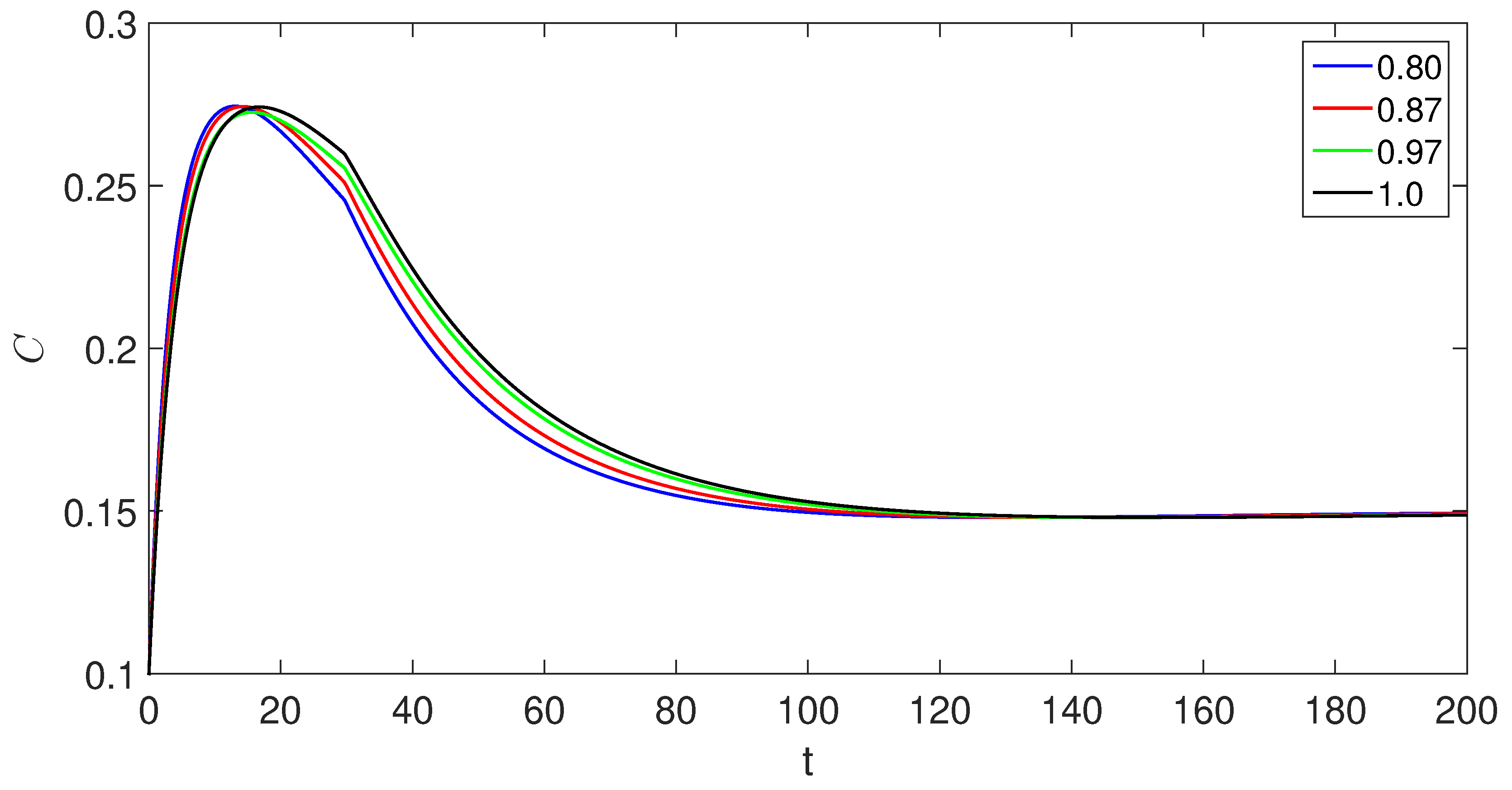
Case (3) When
We have used and plotted the results graphically in Figure 11, Figure 12, Figure 13, Figure 14 and Figure 15 for various fractional orders which are graters in the first two cases here. The concerned transmission dynamics of various compartments has been shown. We see the crossover behaviors in each compartments due to piecewise version of derivatives near the point . The declines in susceptible class, exposed classes and the concerned changes in other compartments can be observed easily.
7. Conclusion
We have studied a dynamics system of a Hepatitis B virus (HBV) with the class of asymptomatic carriers with some new perspectives of fractional calculus. We have used piecewise derivatives of fractional orders with non-local kernel as well as singular kernel. We have established some appropriate conditions for the existence of such models using the tools of nonlinear analysis. In addition, for numerical illustration, we have used Adam Bashforth numerical method. Using the real values of parameters already reported the concerned results have been presented graphically under various fractional orders. The model numerical demonstrated the crossover effect in the dynamics using the time domain for transmission near the point where . The mentioned aspects of fractional calculus has recently recognized a powerful tool to elaborate the sudden or abrupt changes in the real world phenomenon with more brilliant ways. In the future, we will use this methodologies in other complex dynamical models of other diseases.
Age-specific data reveals that acute HBV infection is typically asymptomatic in infants, young children (under the age of 10), and immunocompromised adults. Symptomatic cases are more common among adults and older children, accounting for approximately 30 to 50% of infections. Although research suggests that individuals infected with HBV without symptoms can still transmit the virus and may face the risk of liver damage or even death, particularly if they remain asymptomatic for over six months
Funding
Not applicable.
Availability of data and material
The authors declare that all data and materials in this paper are available and veritable.
Conflicts of Interest
The authors declare that they have no known competing financial interests or personal relationships that could have appeared to influence the work reported in this paper.
References
- Volterra, V.: Théorie mathématique de la lutte pour la vie. Gauthier-Villars, Paris (1931).
- Lotka, A.J.: Elements of Physical Biology. Williams & Wilkins, Baltimore (1925).
- Kolmogoroff, A.N.: Sulla theoria di Volterra della lotta per l’esistenza. G. Ist. Ital. Attuari 7, 74–80 (1936).
- Kostitzin, V.A.: Mathematical Biology. Harrap, Bromley (1939).
- Smith, M.: Models in Ecology. Cambridge University Press, Cambridge (1974).
- Murray, J.: Mathematical Biology. Springer, Berlin (1989).
- Svirezhev, Y.M.: Nonlinearities in mathematical ecology: phenomena and models, would we live in Volterra’s world. Ecol. Model. 216, 89–101 (2008). [CrossRef]
- Kilbas, A.A., Shrivastava, H.M., Trujillo, J.J.: Theory and Applications of Fractional Differential Equations. Elsevier, Amsterdam (2006).
- Podlubny, I.: Fractional Differential Equations. Academic Press, San Diego (1999).
- Caputo, M, Fabrizio, M: A new definition of fractional derivative without singular kernel. Prog. Fract. Differ. Appl. 1(2), 73-85 (2015). [CrossRef]
- Atangana, A, Baleanu, D: New fractional derivative with non-local and non-singular kernel. Therm. Sci. 20(2), 757-763 (2016).
- Abdeljawad, T.: A Lyapunov type inequality for fractional operators with nonsingular Mittag-Leffler kernel. J. Inequal. Appl. 2017(1), 130 (2017). [CrossRef]
- T. Abdeljawad, D. Baleanu, On fractional derivatives with generalized Mittag-Leffler kernels, Adv. Differ. Eqs. 2018 (2018) 468. [CrossRef]
- T. Abdeljawad, Fractional operators with generalized Mittag-Leffler kernels and their differintegrals, Chaos 29 (2019), 023102. [CrossRef]
- T. Abdeljawad, Fractional difference operators with discrete generalized Mittag-Leffler kernels, Chaos Sol. Fract. 126 (2019) 315–324. [CrossRef]
- Atangana, A., Gómez-Aguilar, J.F.: Fractional derivatives with no-index law property: application to chaos and statistics. Chaos Solitons Fractals 114, 516–535 (2018). [CrossRef]
- Atangana, A.: Fractal-fractional differentiation and integration: connecting fractal calculus and fractional calculus to predict complex system. Chaos Solitons Fractals 102, 396–406 (2017). [CrossRef]
- Khan, H., Alam, K., Gulzar, H., Etemad, S., Rezapour, S. A case study of fractal-fractional tuberculosis model in China: Existence and stability theories along with numerical simulations. Mathematics and Computers in Simulation, 198 (2022) 455-473. [CrossRef]
- Atangana, A., Baleanu, D.: New fractional derivatives with nonlocal and nonsingular kernel: theory and application to heat transfer model (2016). arXiv:1602.03408. arXiv preprint.
- Khan, A., Gómez-Aguilar, J. F., Khan, T. S., Khan, H. Stability analysis and numerical solutions of fractional order HIV/AIDS model. Chaos, Solitons & Fractals, 122, 119-128 (2019). [CrossRef]
- Alkahtani, B.S.T.: Chua’s circuit model with Atangana-Baleanu derivative with fractional order. Chaos Solitons Fractals 89, 547–551 (2016). [CrossRef]
- Abdo, M. S., Abdeljawad, T., Kucche, K. D., Alqudah, M. A., Ali, S. M., & Jeelani, M. B.: On nonlinear pantograph fractional differential equations with Atangana–Baleanu–Caputo derivative. Advances in Difference Equations, 2021(1) (2021) 1-17. [CrossRef]
- Abdo, M. S., Abdeljawad, T., Ali, S. M., & Shah, K.: On fractional boundary value problems involving fractional derivatives with Mittag-Leffler kernel and nonlinear integral conditions. Advances in Difference Equations, 2021(1), (2021) 1-21. [CrossRef]
- Almalahi, M. A., Panchal, S. K., Shatanawi, W., Abdo, M. S., Shah, K., Abodayeh, K.: Analytical study of transmission dynamics of 2019-nCoV pandemic via fractal fractional operator. Results in Physics, (2021) 104045. [CrossRef]
- Atangana, A., & Araz, S. İ. (2021). New concept in calculus: Piecewise differential and integral operators. Chaos, Solitons & Fractals, 145, 110638. [CrossRef]
- Gul, N., Bilal, R., Algehyne, E. A., Alshehri, M. G., Khan, M. A., Chu, Y. M., & Islam, S. (2021). The dynamics of fractional order Hepatitis B virus model with asymptomatic carriers. Alexandria Engineering Journal, 60(4), 3945-3955. [CrossRef]
- Van den Driessche, P., & Watmough, J. (2002). Reproduction numbers and sub-threshold endemic equilibria for compartmental models of disease transmission. Mathematical biosciences, 180(1-2), 29-48. [CrossRef]
- Abdeljawad, T., Baleanu, D.: Discrete fractional differences with nonsingular discrete Mittag-Leffler kernels. Adv. Differ. Equ. 2016(1), 232 (2016). [CrossRef]
- Goufo, E.F.D. Application of the Caputo-Fabrizio fractional derivative without singular kernel to Korteweg-de Vries-Burgers equation, Math Model Anal, 21(2)(2016), 188-98. [CrossRef]
- Losada, J, Nieto, JJ: Properties of a new fractional derivative without singular kernel. Prog. Fract. Differ. Appl. 1(2), 87-92 (2015). [CrossRef]
Figure 1.
Graphical presentations of susceptible individuals for the HBV using given fractional orders.
Figure 1.
Graphical presentations of susceptible individuals for the HBV using given fractional orders.
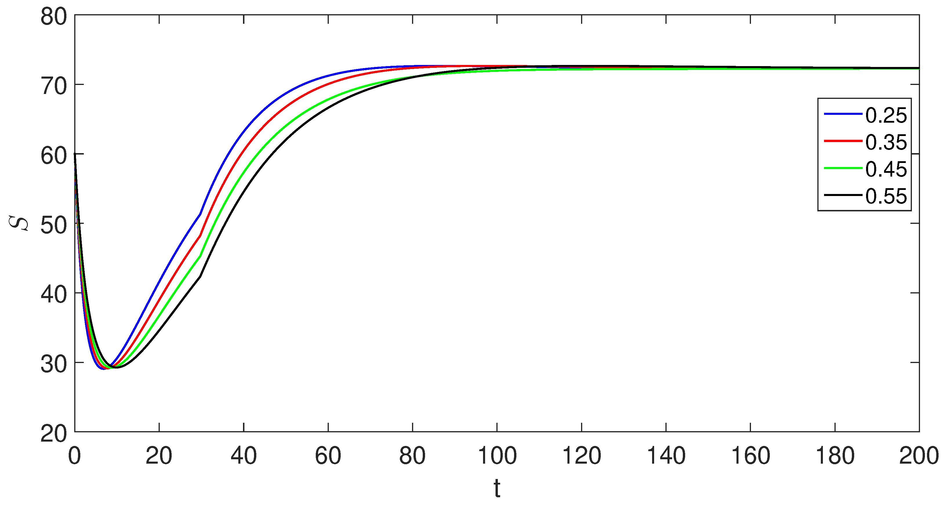
Figure 2.
Graphical presentations of the exposed population for the HBV using given fractional orders.
Figure 2.
Graphical presentations of the exposed population for the HBV using given fractional orders.
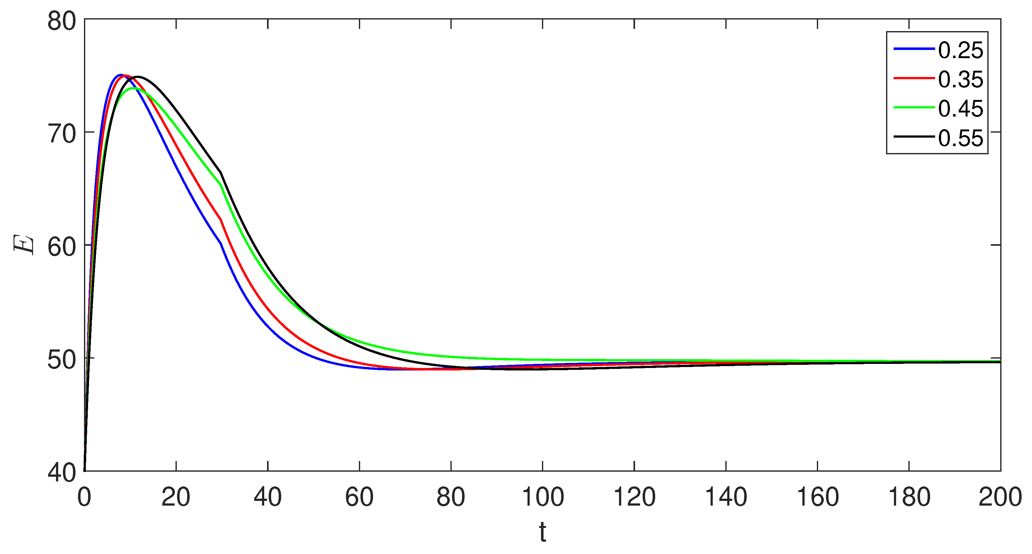
Figure 3.
Graphical presentations of the acute infected population for HBV using given fractional orders.
Figure 3.
Graphical presentations of the acute infected population for HBV using given fractional orders.
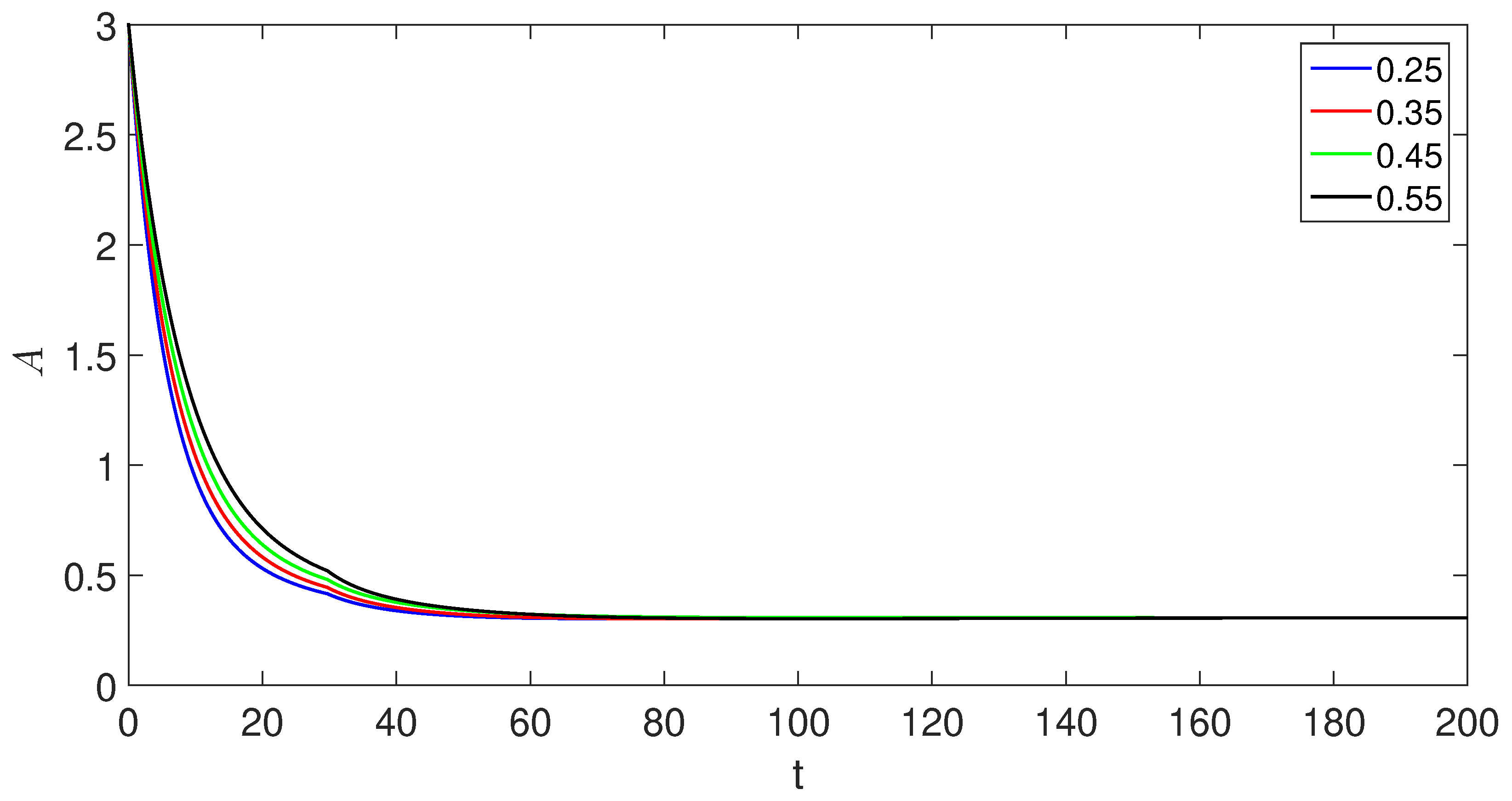
Figure 4.
Graphical presentations of approximate solutions of asymptomatic carrier for the proposed model using given fractional orders.
Figure 4.
Graphical presentations of approximate solutions of asymptomatic carrier for the proposed model using given fractional orders.
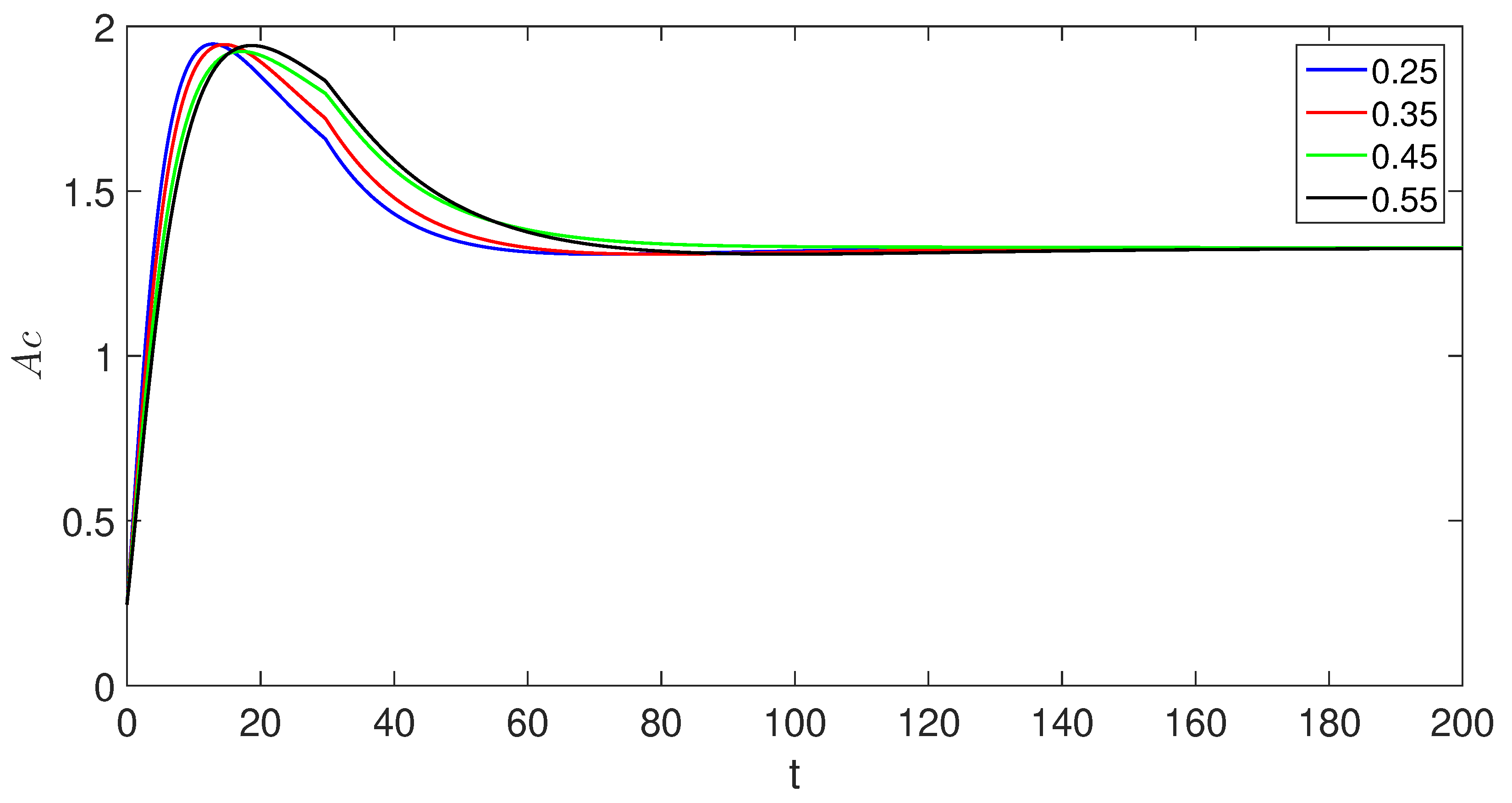
Figure 5.
Graphical presentations of approximate solutions of chronic infected individuals for the proposed model using given fractional orders.
Figure 5.
Graphical presentations of approximate solutions of chronic infected individuals for the proposed model using given fractional orders.
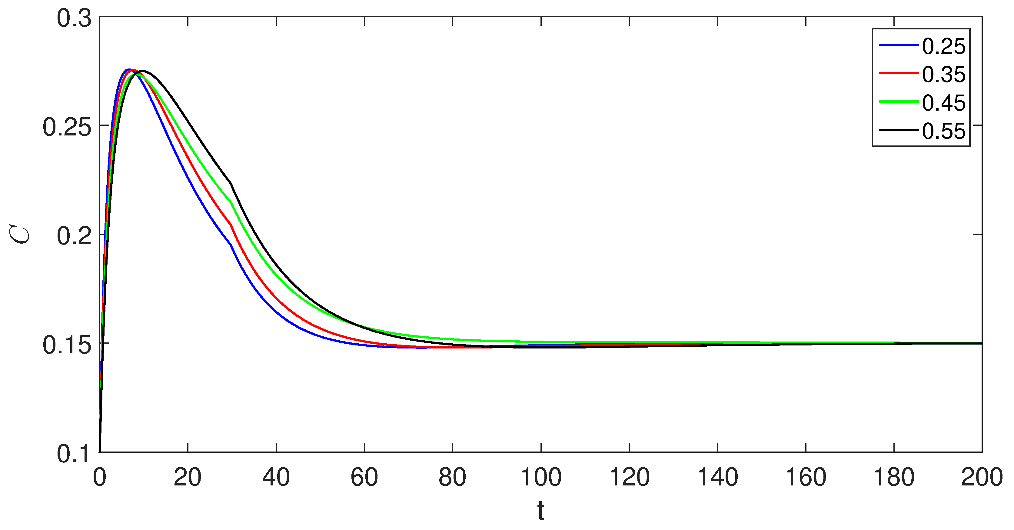
Figure 6.
Graphical presentations of susceptible individuals for the HBV using given fractional orders.
Figure 6.
Graphical presentations of susceptible individuals for the HBV using given fractional orders.
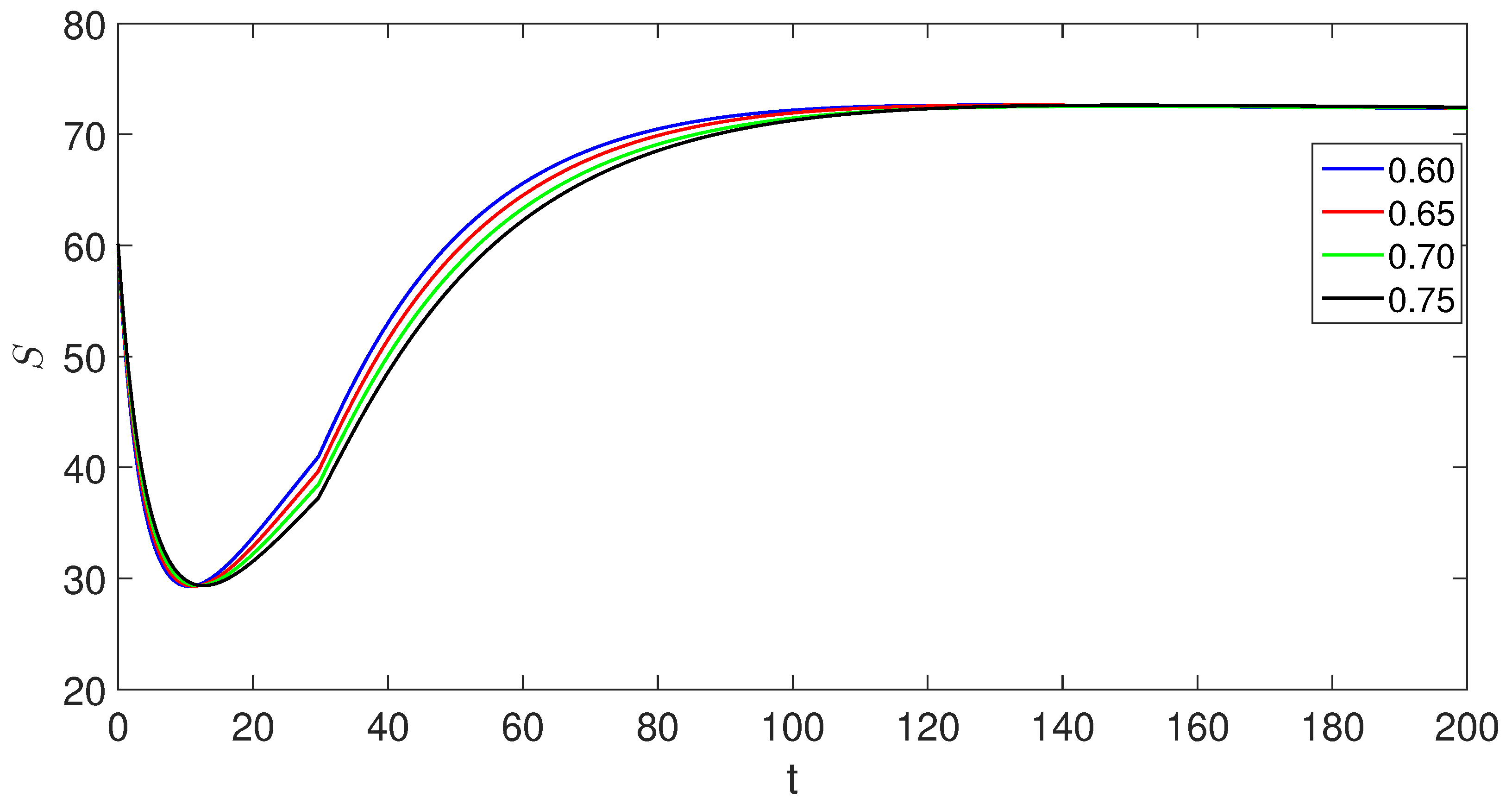
Figure 7.
Graphical presentations of the exposed population for the HBV using given fractional orders.
Figure 7.
Graphical presentations of the exposed population for the HBV using given fractional orders.
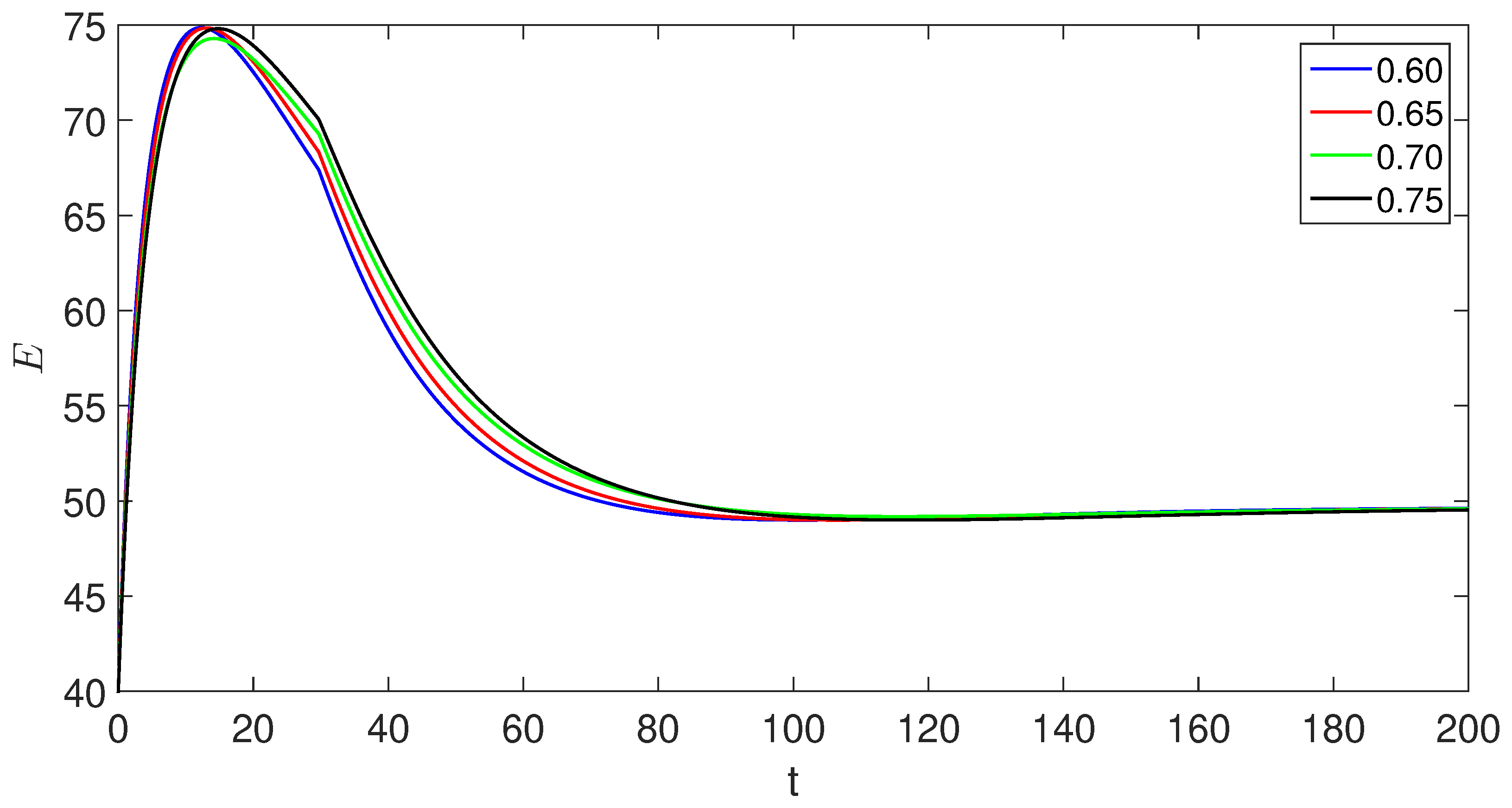
Figure 8.
Graphical presentations of the acute infected population for HBV using given fractional orders.
Figure 8.
Graphical presentations of the acute infected population for HBV using given fractional orders.
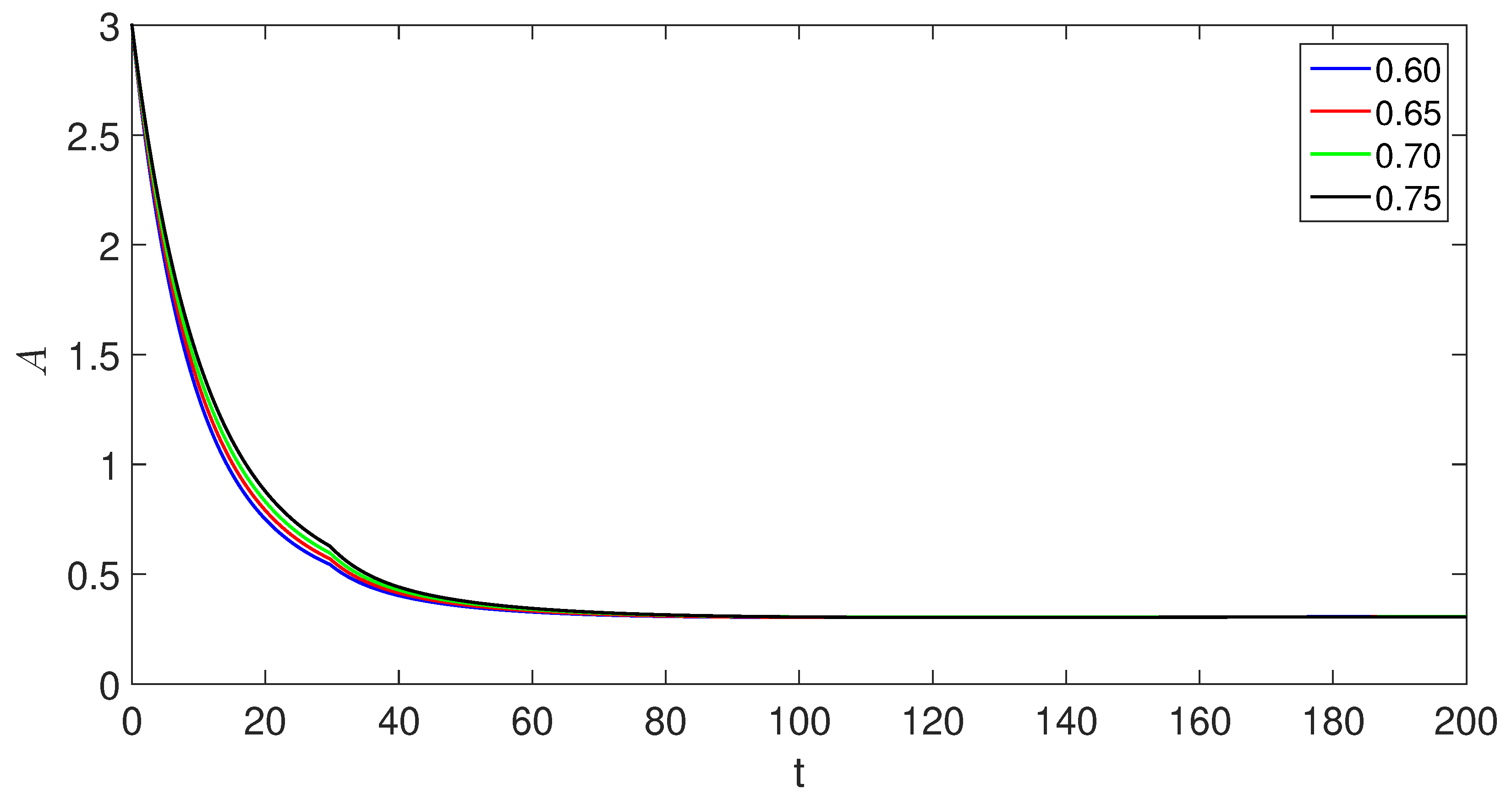
Figure 9.
Graphical presentations of approximate solutions of asymptomatic carrier for the proposed model using given fractional orders.
Figure 9.
Graphical presentations of approximate solutions of asymptomatic carrier for the proposed model using given fractional orders.
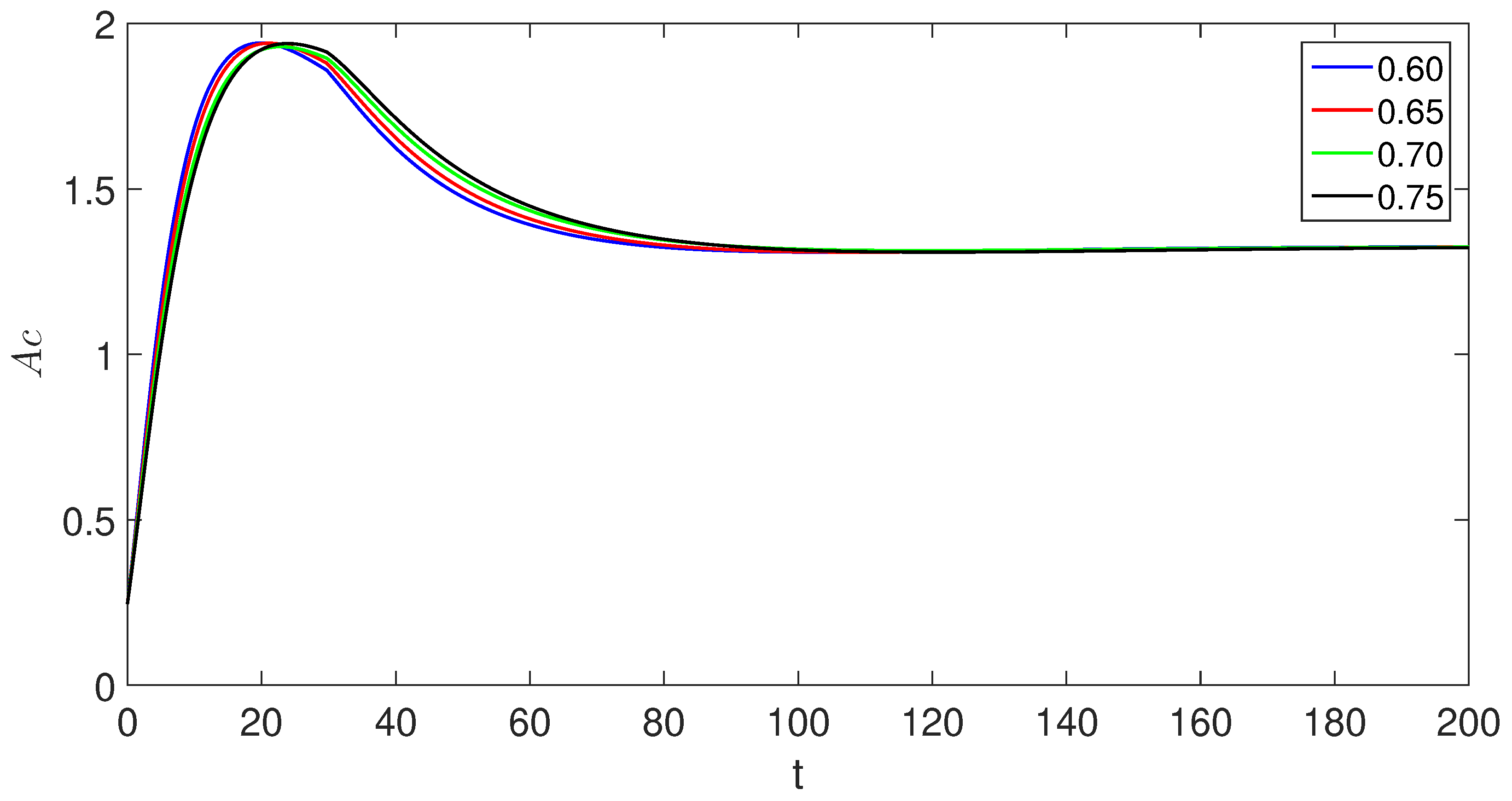
Figure 10.
Graphical presentations of approximate solutions of C for the proposed model using given fractional orders.
Figure 10.
Graphical presentations of approximate solutions of C for the proposed model using given fractional orders.
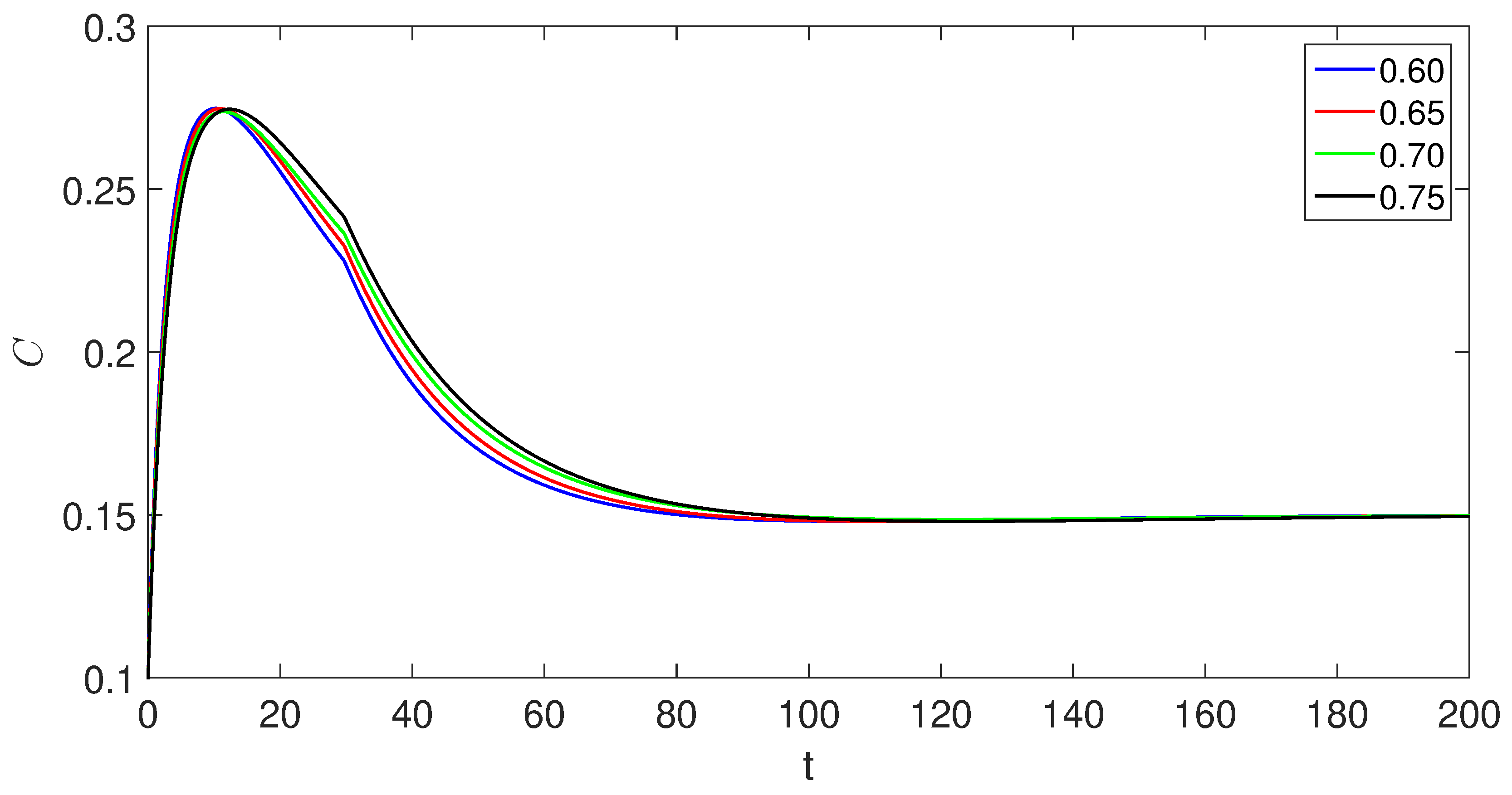
Figure 11.
Graphical presentations of approximate solutions of S for the proposed model using given fractional orders.
Figure 11.
Graphical presentations of approximate solutions of S for the proposed model using given fractional orders.
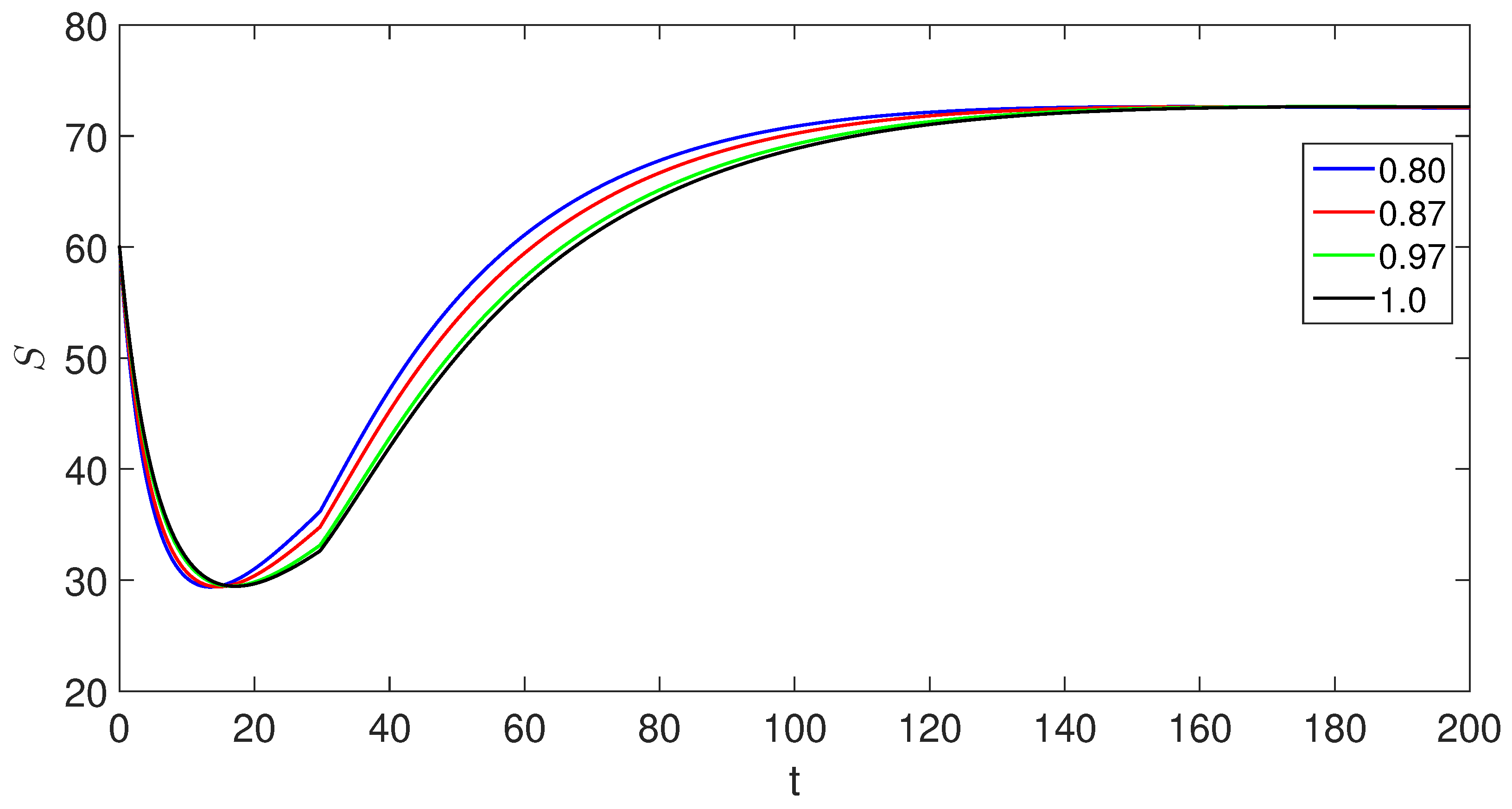
Figure 12.
Graphical presentations of approximate solutions of E for the proposed model using given fractional orders.
Figure 12.
Graphical presentations of approximate solutions of E for the proposed model using given fractional orders.

Figure 13.
Graphical presentations of approximate solutions of A for the proposed model using given fractional orders.
Figure 13.
Graphical presentations of approximate solutions of A for the proposed model using given fractional orders.
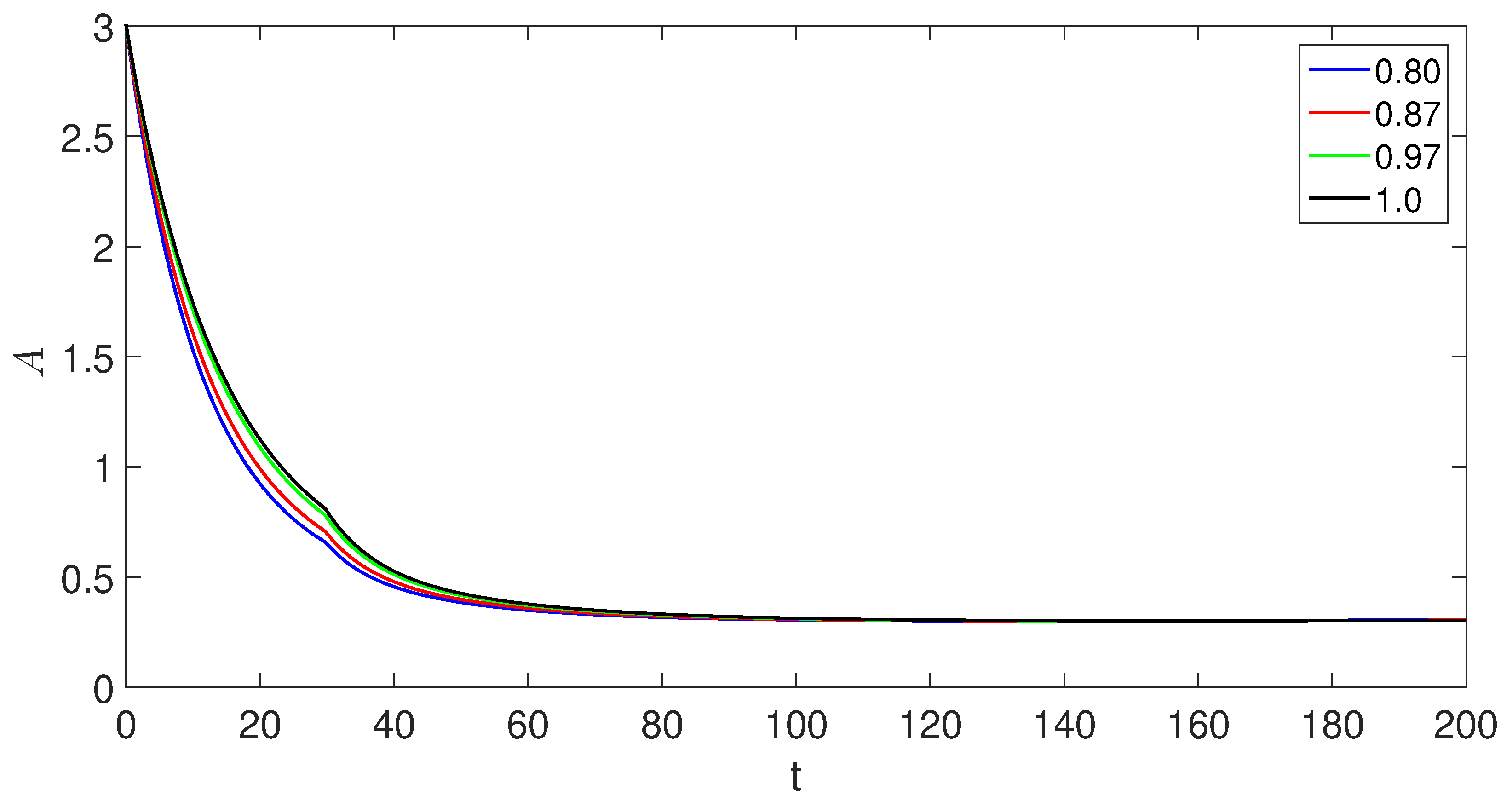
Figure 14.
Graphical presentations of approximate solutions of for the proposed model using given fractional orders.
Figure 14.
Graphical presentations of approximate solutions of for the proposed model using given fractional orders.
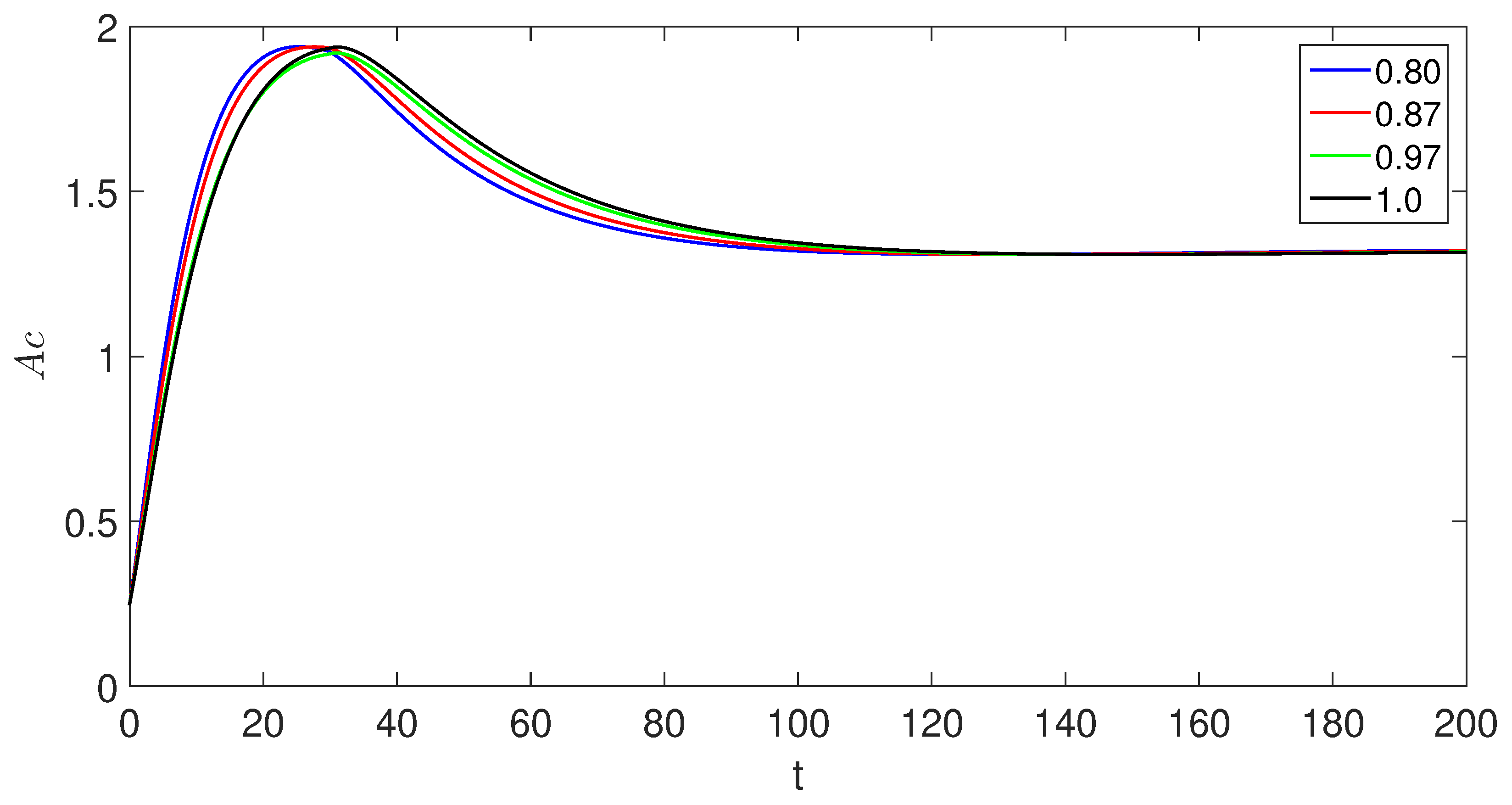
Figure 15.
Graphical presentations of approximate solutions of chronic infected individuals for the proposed model using given fractional orders.
Figure 15.
Graphical presentations of approximate solutions of chronic infected individuals for the proposed model using given fractional orders.
Disclaimer/Publisher’s Note: The statements, opinions and data contained in all publications are solely those of the individual author(s) and contributor(s) and not of MDPI and/or the editor(s). MDPI and/or the editor(s) disclaim responsibility for any injury to people or property resulting from any ideas, methods, instructions or products referred to in the content. |
© 2023 by the authors. Licensee MDPI, Basel, Switzerland. This article is an open access article distributed under the terms and conditions of the Creative Commons Attribution (CC BY) license (http://creativecommons.org/licenses/by/4.0/).
Copyright: This open access article is published under a Creative Commons CC BY 4.0 license, which permit the free download, distribution, and reuse, provided that the author and preprint are cited in any reuse.


