
Submitted:
27 October 2023
Posted:
30 October 2023
You are already at the latest version
Abstract
The distribution laws of various natural and anthropogenic processes in the world around us are stochastic in nature. The development of mathematics and, in particular, of stochastic modelling allows us to study regularities in such processes. In practice, stochastic modelling finds a huge number of applications in various fields, including finance and economics. In this work, some particular applications of stochastic processes in finance are examined in the conditions of financial crisis. More specifically, Autoregressive Integrated Moving Average (ARIMA) models and Modified Ordinary Differential Equations (ODE) models, which have been previously developed by the authors to predict assets’ prices of four Bulgarian companies, are validated on a time period during the crisis. Estimated rates of return are calculated from the models for one period ahead. The errors are estimated and the models are compared. The predicted return values with each of the two approaches are used to derive optimal risk portfolios based on the Markowitz Model. The resulting portfolios are compared in terms of distribution (weights of the stocks), risk and rate of return.
Keywords:
stochastic processes
; time series
; ARIMA
; ODE
; price forecasting
MSC: 60G35; 91B84; 34A34; 34A55; 91B28; 90C90
1. Introduction
Financial markets have always attracted considerable attention due to their critical influence on developed countries economic infrastructure, and also because of their facilitation of huge volumes of capital flow. Functioning as complex systems for the trading of various financial instruments—both domestically and internationally—these markets serve as mainstay for resource allocation and liquidity provision in the broader economic landscape. In contemporary economic theory, financial markets are accredited with six fundamental roles: price determination, liquidity provision, transactional efficiency, facilitation of credit and lending mechanisms, real-time information dissemination on cash flows, and risk management strategies.
To cater to the diverse investment preferences of market participants, various types of financial markets exist. These range from Foreign Exchange Markets, which are arguably the largest of their kind, to Capital Markets trading in shares, bonds, and ETFs. Additionally, Money Markets largely concern short-term financial instruments and are typically dominated by banking institutions. Other categories include Derivatives Markets, Commodities Markets dealing in raw materials, the nascent Cryptocurrency Markets, Mortgage Markets focused on real estate investments, and Insurance Markets that allow for risk transference through premiums. Each of these markets has its own temporal focus—some being more suitable for short-term investments, while others are geared toward long-term holdings.
In Bulgaria, where the Capital Market is yet to reach full maturity, stock price prediction has increasingly become an imperative subject of financial analysis, not just for professional investors but also for the general audience. Within stock markets, the necessity for robust investor education is emphasized due to the market’s inherent volatility and sensitivity to a multitude of variables. Indeed, the dynamics of the market, coupled with various external and internal factors, contribute to rapid fluctuations in the price of traded assets. Publicly available historical data often exhibit predictive correlations with future stock returns; the challenge lies in accurately identifying and utilizing this data for predictive modeling. This challenge is even greater in the conditions of a financial crisis, when there is a worsening dynamics of macroeconomic indicators and increased volatility of financial markets.
In the sphere of portfolio management theory [1], the principle of separation states that given identical input variables, all investors will have the same optimal risk portfolio. This separates the challenge of portfolio selection into two problems. The first is essentially a technical problem that involves the construction of an optimal risk portfolio, which is designed to maximize the reward-to-variability ratio based on input variables like rates of return, standard deviations, and correlation matrices. The second problem necessitates the proportional allocation of risk-free treasury bonds and the aforementioned risk portfolio, contingent upon the individual risk tolerances and preferences of each investor.
In the present research, we delve into specific applications of stochastic processes within the realm of finance, particularly during periods of financial turmoil. Our focus is directed towards the validation of two distinct models: the Autoregressive Integrated Moving Average (ARIMA) and the Modified Ordinary Differential Equations (ODE). These models, previously devised by the authors (see [2,3]) to forecast asset prices for four prominent Bulgarian companies, , have been applyed over a timeline encompassing the financial crisis.
To ascertain the models predictive accuracy, we computed the estimated rates of return for one period ahead. Subsequent to this, the magnitudes of errors [4] were quantified and a comparative analysis between the models was conducted. The forecasted return values procured from both methodologies were instrumental in formulating optimal risk portfolios, grounded in the principles of the Markowitz Model. A meticulous examination of these portfolios was undertaken, considering variables such as asset distribution, inherent risk, and estimated rate of return.
2. Materials and Methods
2.1. ARIMA Models
In contemporary financial analytics, Autoregressive Integrated Moving Average (ARIMA) models have been extensively harnessed to extrapolate potential trajectories for stock prices, anchored primarily on their historical performance, or to project a company’s future earnings by scrutinizing previous fiscal intervals. These analytical structures are anchored in the broader spectrum of regression studies, proficiently elucidating the relative potency of a chosen dependent variable in contrast to other evolving determinants. Fundamentally, the ARIMA methodology aspires to forecast impending shifts in securities or broader financial market trajectories. Intriguingly, this is accomplished not by direct examination of absolute values but rather by analyzing the variances between consecutive data points in a series.
The construction of ARIMA models pivots around three parameters, colloquially denoted as p, d, and q [5]. The autoregressive component, symbolized by ‘p’, encapsulates the influence exerted by data from ‘p’ antecedent intervals within the analytical framework. Conversely, the integrated component, represented by ‘d’, captures the overarching trend manifest in the dataset. The moving average segment, denoted by ‘q’, delineates the number of sequential data points that are leveraged to temper minor oscillations using a moving average methodology.
To encapsulate the theoretical construct, an ARIMA model with the specified parameters p, d, and q, as cited in references [5,6], can be mathematically represented as per equation (1):
Here are the parameters sought, is a randomly distributed variable with mathematical expectation of zero and dispersion . If we do not have any information about the distribution of this variable, then by default it is assumed that the distribution is normal [6]. ∆ is the difference operator, which is defined as (2):
In this study, we have experimented with diverse permutations of the parameters (p, d, q) with the intent of meticulously characterizing the underlying time series dynamics. The graphical representations of auto-correlation functions (ACFs) and partial auto-correlation functions (PACFs) for each unique parameter combination are reviewed. These functions are predicated upon a predetermined number of lags and are systematically computed for every temporal juncture ‘t’, barring certain terminal instances where their derivation proves infeasible.
Critical to our assessment is the scrutiny of discontinuities or ‘jumps’ manifested within both the ACF and PACF. These fluctuations serve as invaluable markers, guiding the optimal selection of parameters for each model. It’s noteworthy that if for a given Yt both ACF and PACF portray either an absence of jumps or a singular, marginal deviation beyond the confines of the 95% confidence intervals, such a model is adjudged to be adequately robust and congruent with the research objectives delineated in this study.
The formula for the autocorrelation function ACF in the current moment ‘t’ for a ‘k’ lag can be articulated as per equation (3):
Here n is the number of observations in the time series; k is the delay, calculated as number of lags; is the mean value of the time series. The denominator represents the dispersion of the time series. The standard autocorrelation error is based on the square of the autocorrelation of all previous autocorrelations.
In the given context, n denotes the total count of observations present within the time series, while k signifies the lag, quantified in terms of the number of time delays. stands as the arithmetic mean of the entire time series. The denominator encapsulates the variance inherent to the time series. The canonical error associated with autocorrelation is derived from the squared magnitude of the autocorrelation spanning all preceding autocorrelations.
The mathematical representations for ascertaining partial correlations are intrinsically intricate, necessitating the application of recursive methodologies [7].
2.2. Modified ODE Models
In those cases, where extensive datasets are utilized, the application of more intricate forecasting techniques based on numerical solutions for ordinary (ODE), partial (PDE), and stochastic (SDE) differential equations becomes imperative [8,9,10].
This article investigates a modified ODE methodology for simulating the price fluctuations of a specific asset over a defined period. The benefits of this adaptation are illustrated through numerical examinations. Market data encompassing the daily closing prices of the Alterco instrument (A4L), ranging from June 1, 2020, to October 28, 2020, has been employed for this purpose. Numerical models derived for price forecasting are based on the numerical resolution of the Cauchy initial problem for the first-order ODE. The computational attributes of the modified ODE are analyzed using Matlab [11]. The computational tests involve an array of data fitting models to determine the optimal predictive values, computed as the weighted average of all projections for the respective instruments. The weights are inversely correlated to the "final errors."
Consider the chronologically organized moments in ascending order, along with the observed values for an asset, represented as a time series, as indicated in (4):
As demonstrated in prior studies [8,9], it is feasible to calibrate an ordinary differential equation to this particular time series.
describing the discrete time points of the time series values provided. The function g(t, y) can be significantly diverse.
In the scenario where , equation (5) can be addressed either through numerical integration or by acquiring an analytic solution, provided that the value of is known. It is also plausible to calibrate the variable at various time intervals. One method for resolving equation (5), with , is delineated by Lascsáková in [9]. Another approach, presented by Xue and Lai [8], introduces several alternatives in the structure of the first derivative in (5). They suggest the subsequent form for
Here, and are representable by elementary functions such as polynomial functions, exponential functions, logarithmic functions, and the like. They can be expanded to include series of degrees subject to specific conditions. Furthermore, within the dataset (4), discernible periodic trends can be identified. Consequently, the function in the structure of (6) could potentially comprise a polynomial aspect along with a trigonometric component.
Let us consider the scenario where the first derivative is in the following format:
i.e.
The parameters under consideration are the coefficients:
The number of these coefficients is . If the condition (which will be assumed to always hold) is satisfied, they can be determined by resolving an inverse problem using a numerical method involving a one-step explicit or implicit approach (or a combination of the two):
Here , while denotes the right-hand side of (5), and signifies a specific one-step numerical method, such as explicit or implicit Euler, Runge-Kutta, among others. As demonstrated in [8], one can utilize the last values of the time series (4). Employing (10) leads to the establishment of a system of nonlinear equations concerning the coefficients (9). Once this system is solved, the said coefficients (9) can be determined. These coefficients are then employed to define the forthcoming unknown value, , at time instant . In equation (5), all coefficients are already known, enabling the computation of the next value through the numerical method .
One limitation of this methodology is its failure to utilize the complete information embedded within the time series (4). As per this approach, only as many values are extracted from series (4) as necessary to close the system of nonlinear equations, determined by the specific selection of and . However, this shortcoming is effectively circumvented in this research, wherein any number of values can be selected (when ) from line (4). Subsequently, the over-determined system of nonlinear algebraic equations is solved through the application of the Least Squares Method (LSM). The LSM can also be applied in a weighted format, allowing for the incorporation of a weight function. It stands to reason that the weight function should assign higher weights to the more recent values in the time series (4), thus demonstrating an increasing trend or, at the very least, remaining constant.
Within the context of this paper, the weight of the errors in the Least Squares Method (LSM) is determined by the ascending function:
Various experiments have been conducted at diverse weight values of (at the function (11) is convex, at – concave). To be precise, the weights (12) have been employed in lieu of the weight function (11).
The utilization of (12) is motivated by the assignment of a weight to each error within the range of [0,1]. A weight of 0 is assigned to the data point furthest in time, while the closest (most recent) data point is assigned a weight of 1. This selection process is primarily subjective, allowing for the potential use of varying weights, provided they follow an increasing pattern.
The predicament arises when employing LSM (9) to define the coefficients, resulting in the resolution of a nonlinear system of algebraic equations. It is widely acknowledged that nonlinear systems can yield multiple solutions, and different selections among these solutions can lead to diverse predictions [12].
Due to the inherent nonlinearity of the system, it is not feasible to ascertain beforehand the exact number of solutions it may offer. When employing a specific numerical method to solve the nonlinear system concerning the coefficients (9), initial approximations for these coefficients are provided. Different choices of initial approximations typically result in varied solutions. In this study, the approach involves the selection of different initial approximations:
The generated solutions are determined pseudo-randomly, with each value assigned to a pre-selected interval. These distinct solutions are isolated. To select a specific solution from this set, the last values from the time series are extracted and segregated to create an error, which then validates a chosen solution of (9). These designated values are referred to as "test values." The subsequent value is predicted and contrasted with the actual value, subsequently incorporating the real value back into the time series and recording the corresponding error. This process is carried out sequentially for these values of the time series. The "final error" is computed as the weighted average of the errors obtained, whereby an increasing function may once again be employed as the weighting function. The solution of (10) yielding the smallest "final error" is selected to define (10) for a specific choice of and . Subsequently, the future value at time is predicted.
The solution for the over-determined system of nonlinear equations can also be achieved through the minimax method, ensuring minimal maximum error between the approximated and actual values. Additionally, the weighted minimax method can also be applied in this case.
To summarize the approach for predicting the subsequent value in the time series at given intervals and given time series values (4):
1. Fit an ordinary differential equation with initial condition (5) - a Cauchy problem to the time series.
2. Choose the form (7) for the function by fixing the parameters and .
3. Select a specific numerical method - such as explicit, implicit, or a combination of both, including one-step methods like Euler, Milne, Runge-Kutta, etc. - for the numerical solution of (5).
4. Select the last values of the time series (4) (where ).
5. Solve an inverse problem with respect to the unknown coefficients (9), which reduces to solving an over-determined system of nonlinear equations.
- Choose a method to minimize the given error for solving the over-determined system - whether it’s LSM, the minimax method, or a similar approach.
- Select a weight function to implement this method, ensuring the weight function is non-decreasing (in this specific case, of type (12)).
- Apply the chosen method with the selected weight function to reduce the over-determined system to a nonlinear system of equations.
- Due to the nonlinearity of the obtained system, generate different pseudo-random initial approximations (13) for the coefficients (9) and obtain different solutions for (9).
6. Select the last values of (4) and segregate them to construct an error and validate the chosen solution of (9). Compute the "final error" as a weighted average of the errors obtained, where the weights are increasing.
7. Choose the solution of (9) with the smallest "final error."
8. Substitute the chosen solution of (9) into (10) and predict the future value at time for .
9. Repeat steps 1-8 for different choices of: the numerical method used to solve the initial Cauchy problem, the parameters , , , , , the numerical method for solving the over-determined system of nonlinear equations, the weight function for solving the over-determined system of nonlinear equations, and the weight function for estimating the "final error."
10. After obtaining different forecasts and their "final errors," compute their weighted average value, with weights being inversely proportional to their "final errors," and consider it as the final forecast.
2.3. Risk Portfolio Optimization
The authors utilize a previously established Matlab programming code [13] to generate an efficient risk portfolio comprising a set of volatile securities. The primary objective is to maximize the Capital Allocation Line (CAL) for every eligible risk portfolio labeled as . The code effectively resolves the optimization problem (14) while adhering to the specified condition (15):
where:
- - weight of the i-th asset,
- - the anticipated return rate of the risk portfolio refers to the average value of the expected return rates of the volatile assets, weighted by their respective proportions within the risk portfolio. This value is computed in accordance with the demonstration provided in (16).
- – the standard deviation, calculated as shown in (17).
- – the correlation coefficient between the i-th and the j-th asset rates of return.
The resolution of the optimization problem relies on a modified version of the Markowitz model [14] predicated on the following assumptions: the presence of risk-free assets, the ability to borrow at a risk-free rate, and the opportunity for short sales of volatile assets.
The input data provided for the developed programming code encompasses projected return estimates, their respective deviations from the mean, the corresponding correlation matrix, and the return rate for risk-free assets. The resulting output from the program comprises an optimized risk portfolio for assets over a single period, along with an estimation of the expected return for the designated risk portfolio.
The programming code itself is listed below.
function [S,W_p,Er_p, StD_p]=fopt_portfolio(ERoR,StD,CM,RoRf)
% %% INPUT DATA %%%
% ERoR – Expected Rate of Return (RoR) – n-dimensional vector
% StD - Standard Deviation of RoR – n-dimensional vector
% CM - Correlation Matrix – nxn matrix
% RoRf – RoR of the risk-free asset
n=length(ERoR);
ERoR=ERoR(:);
StD=StD (:);
% CovM - Covariance Matrix
CovM=( StD*StD').*CM;
% F = -S – optimization function
F=@(w)-(w(:)'*ERoR-RoRf)./sqrt(w(:)'*CovM*w(:));
% w - vector of weights
% Search that w, where min(F)
[W_p,S]=fmincon(F,ones(n,1)/2,[],[],ones(1,n),1,zeros(n,1),ones(n,1));
%%% OUTPUT DATA %%%
Er_p=W_p'*ERoR;S=-S;
% W_p - weights in the optimal risk portfolio
% Er_p - Estimated RoR of the optimal risk portfolio
StD_p=sqrt(W_p'* CovM*W_p);
% StD_p - Standard Deviation of RoR of the optimal risk portfolio
In the present work, the problem of creating a portfolio of equities of the four companies and treasury bills is solved. The horizon of the portfolio plan is one period ahead. All estimates refer to the rates of return for one period of ownership.
The assets’prices from 29.10.2020 (respectively, 28.10.2022) are taken as the prices for a moment of time 0. The set of expected rates of return is calculated as shown in (18):
where – the prices at time 0 , - the estimated prices from the obtained models at time 1 (30.10.2020, and respectively 31.10.2022).
In the context of the implemented program, the calculations disregard the signs preceding the return rates. However, during the interpretation of the outcomes, this sign is employed to determine whether to engage in a short (negative) or a long (positive) position regarding that specific asset.
3. Results
The investment portfolio comprises a combination of shares from four Bulgarian companies operating in distinct sectors, namely technology, real estate, courier/transport services, and finance. These companies include the technology holding Allterco JSC, the joint-stock company Elana AgroCredit JSC, the courier company Speedy JSC, and the holding Chimimport JSC. A daily data for the period 01.06.2020-29.10.2020 is used for the development of the models, and a daily data for 01.06.2022-29.10.2022 is used for their validation. The data is taken from Bulgarian Stock Exchange [15]. Table 1 and Table 2 show the financial results of the four companies, respectively to the end of 2020 and 2022.
Allterco JSC - Sofia Allterco Robotics is a well-established firm in the telecommunications and smart technology domain, having commenced operations in 2010 in Sofia, Bulgaria. It has gained recognition as an innovative enterprise focusing on the development and trade of IoT (Internet of Things) devices. Notable products include the widely popular MyKi smartwatches for children and the Shelly technology tailored for household applications. The company’s shares were officially listed on the Bulgarian Stock Exchange (BSE) on December 1, 2016.
Elana AgroCredit JSC - Sofia REIT (Real Estate Investment Trusts) provides agricultural loans to farmers for the acquisition of farming land, facilities, and advanced technologies. It stands as the pioneering entity specialized in financial leasing. The company’s shares have been publicly traded on the BSE since the latter part of 2013.
Speedy JSC, established in 1998, has emerged as a prominent courier enterprise in Bulgaria. Its strategic partnership with DPD, Europe’s largest ground delivery network, has significantly contributed to its successful global deliveries. Currently holding a substantial market share of 25.5%, Speedy became the first company in its industry to go public when it was listed on the BSE in November 2012.
Chimimport JSC, established in 1947 as an external holding, focuses on the chemical products market. The conglomerate includes over 68 successful companies renowned in various sectors such as banking services, insurance, pension fund management, mutual fund management, as well as receivables and real estate securitization. Chimimport JSC is dedicated to providing comprehensive financial services and a diverse range of operations to cater to its clientele.
3.1. Models Development
3.1.1. ARIMA Models Development
Using the daily closing prices of the instruments Alterco (A4L), Chimimport (CHIM), Elana AgroCredit (EAC), and Speedy (SPDY) from the period 01.06.2020 - 29.10.2020 (151 periods – from 0 to 150, including weekends and missing data), diverse predictions are generated using the ARIMA approach for the closing price value on the following day, i.e., October 30, 2020. A subset of the last known six periods () is reserved for validation purposes.
The development sample for each instrument encompasses data excluding the validation periods specific to the corresponding instrument. Successful models identified in the development sample undergo incremental testing by integrating the validation periods step by step. Calculations are made for the errors derived from the predictions at each step, which are then employed to compute the weighted average error, adhering to the principle that recent observations bear greater significance.
A careful examination is conducted to ascertain whether the models, when applied to the development and validation data, exhibit any significant deviations beyond the 95% confidence intervals in the ACF (Autocorrelation Function) and PACF (Partial Autocorrelation Function) residual graphs. If no substantial deviations or minor discrepancies are observed, the model is applied to the complete dataset for the relevant instrument, thus producing the predicted value for one period ahead.
For each period during which the respective models undergo validation, forecast errors are computed. The outcomes are systematically presented in Table 2, Table 3, Table 4 and Table 5. Notably, data for periods 145 and 146 (October 24, 2020, and October 25, 2020) are absent due to these days falling on weekends (when financial exchanges are closed). Additionally, data gaps exist for certain instruments even during working days, as explained in detail below.
Regarding A4L (as presented in Table 3), there is an absence of data for period 150, corresponding to October 29, 2020.
Regarding CHIM (Table 4), there is an absence of data for period 144 (23.10.2020).
Regarding EAC (as presented in Table 5), there is an absence of data for period 147, corresponding to October 26, 2020.
Regarding SPDY (as shown in Table 6), there were no instances of missing data for the working days within the examined validation period.
The aim is to generate a forecast for . The computation of the weighted average error is conducted as follows: the assigned weights for computing the weighted average error were . These weights correspond to the errors in the retained validation cases. The weight allocation is determined subjectively, based on a linear function established through empirical observation. The latter error is given 1.5 times the weight of the former. Table 7 provides the projected values and weighted average errors for the selected models for each of the four financial instruments, respectively.
For example, for the first instrument – A4L, the weighted average error for the model ARIMA (2,1,6) from Table 7 is derived from Table 3 as shown in (19):
The remaining weighted average errors are computed in a similar manner.
A linear combination of the predictions for the two models is employed for each instrument to derive the ultimate projected value. The coefficients in this linear combination are inversely correlated with the weighted average errors obtained from the specified models. The findings are outlined in Table 8.
For example, the projected price for the instrument A4L on October 30, 2020, is derived from Table 7, as illustrated in (20):
3.1.2. Modified ODE Models Development
Similarly to the ARIMA approach, to select a definitive solution from the array of potential solutions, the preceding values (in this instance, data points, factoring in the period in which they are absent) are chosen from the time series and divided to create an error and authenticate a designated solution of (5). These values are referred to as "test values." The subsequent value is anticipated and juxtaposed with the actual value, following which the real value is incorporated back into the time series, and the error value is documented. This process is consistently repeated for those values in the time series. The "final error" is computed as the weighted average error of the 6 errors obtained. Once again, an increasing function can be selected as the weighting function. The solution of (5) with the minimum "final error" is employed to construct (6) based on a specific choice of and Subsequently, the future value of at time is predicted.
On the same data, used for the ARIMA approach, multiple projections have been generated for each instrument based on the different values of and in the modified ODE approach. In solving the nonlinear system of algebraic equations by Least Squares Method, a linear increasing weight function has been chosen. Linear increasing weights were also used in the calculation of the “final error”.
The results of the predictions and the “final errors” for each set of parameters and are given in the Table 9, Table 10, Table 11, Table 12, Table 13, Table 14, Table 15 and Table 16.
The ultimate forecasts are computed as a weighted mean of all predictions for the individual instruments. The weights are reciprocally correlated to the "final errors". Table 17 exhibits the ultimate forecasts (estimated values), the real values, and the percentage relative error between the predicted and actual closing price values for the various instruments as of 30th October 2020. Notably, the prognostications demonstrate exceptional precision (with a maximum relative error of less than 0.6%).
3.2. Models Validation
Data from 2022 is used to validate the models, obtained on the data from 2020. The purpose is to check the behaviour and the robustness of the models in the condition of finantial crisis. The methodology, used on the data from 2020, is applied on the recent data from 2022. This includes building the same models, using the daily closing prices of the instruments A4L, CHIM, EAC, and SPDY from the time window 01.06.2022 - 29.10.2022 (150 periods – from 0 to 149, including weekends and missing data). The last known periods are kept for validation in order to calculate the corresponding errors. Forecasts for 31.10.2022 are obtained (30.10.2022 is Sunday, and therefore this time the prediction is for 31.10, which is Monday).
3.2.1. ARIMA Models Validation
Drawing a parallel to the ARIMA methodology employed in 2020, the present study adopted a sequential validation approach for the period of 01.06-20.10.2022. When a model demonstrated satisfactory performance on this development sample, it underwent further testing by progressively including the validation periods of 21.10-30.10.2022, which comprised six distinct periods when weekends are excluded. Following this, prediction errors were computed at each incremental step. These errors subsequently informed the computation of a weighted average error, which was then applied to the predictions for 31.10.2022.
Diagnostic checks carried out on both the development and validation data for 2022 affirmed the robustness of the existing models. Notably, these models exhibited no discernible anomalies or jumps that exceeded the boundaries of 95% confidence intervals in their ACF and PACF residual plots. Given this affirmation of model stability, they were then deployed on the comprehensive data set spanning 01.06-30.10.2022 for the pertinent financial instrument. The consequent predicted value for 31.10.2022 was subsequently extracted. The outcomes of this exercise are elucidated in Table 18. It is imperative to note that, in instances where data was absent on account of weekends, such omissions were categorized as "no deals", implying the price remained unchanged from the preceding day.
The weighted average error is derived as shown in (19) for the data from 2020. Table 19 shows the predicted values and weighted average errors on the chosen models, applied on the data for 2022.
Similarly, to the methodology on the data from 2020, here a linear combination of the forecasts for 31.10.2022 from the two models for each instrument is used to obtain the final predicted value for the corresponding instrument. The coefficients in this linear combination are inversely proportional to weighted average errors from the given models. The results are presented in Table 20.
3.2.2. Modified ODE Models Validation
Using the similar approach as in Section 3.1.2, and the same values for and , estimates for the prices and final errors are made for 31.10.2022. The results are given in the Table 21, Table 22, Table 23, Table 24, Table 25, Table 26, Table 27 and Table 28.
The final predictions are derived as a weighted average of forecasts across all individual financial instruments. Intriguingly, these weights are inversely related to the "final errors." Table 29 showcases these definitive forecasts (anticipated values), juxtaposed against the actual values, alongside the percentage discrepancy between the forecasted and realized closing prices of the instruments as of 31th October 2022. It’s noteworthy to mention that the forecasts exhibit remarkable accuracy, manifesting a maximal relative deviation of under 2.6%.
3.3. Risk Portfolio Optimization
The programming code from Section 2.3 is applied, using the input data from 2020 and 2022, respectively. This data includes: the estimates of the expected rates of return (Table 30), obtained as a relative difference between the estimated value for 30.10.2020 (respectively, 31.10.2022) and the real value for 29.10.2020 (respectively, for 28.10.2023); the standard deviations, calculated using historical data (Table 30); the correlation matrix, based on historical data (Table 31 for 2020, respectively Table 32 for 2022); the return of the risk-free asset.
For 2020, a government securities with an annual yield of 3%, which is equivalent to 0.0083% daily yield (3% / 360) had been used. For 2022 the annual yield of the government securities was 4.36%, or 0.0121% daily yield.
It can be seen from Table 30 that the expected rates of return differ not only in years (2020 against 2022), but also in type of models. The ARIMA predictions for 2022 (Table 30, Column 5) for A4L, CHIM and SPDY confirm the movement (increase/decrease) observed in the ARIMA predictions from 2020 (Table 30, Column 2), while that for EAC is not confirmed – it undergoes an increase of 0.125% in 2020, but a decrease of 0.4714% in 2022. Modified ODE predictions show that we have confirmation of the movement only for EAC. From the second and the third column of Table 30 it can also be notised that the ARIMA and the Modified ODE approaches predict the same trend (increase) in 2020 for CHIM and EAC and have discrepancy for A4L and SPDY, while in 2022 we have same trend predictions only for A4L. The standard deviations for the two periods (Table 30, Columns 4 and 7) show that EAC is much more risky instrument for 2022 (7.1734% standrard deviation), than for 2020 (1.2198% standard deviation).
The correlation matrixes for the two periods (Table 31 and Table 32) also indicate different movements and connections between the companies in the time window in 2022, compared to that in 2020.
The results obtained with the optimization code are as follows. The optimal risk portfolio for 30.10.2020, constructed using ARIMA predictions (Figure 1(a)) consists of: 19.23% shares in A4L in a long position; 8.37% shares in CHIM in a short position; 7.20% shares in EAC in a long position, and 65.21% shares in SPDY in a short position. The portfolio for the same data, constructed using Modified ODE predictions (Figure 1(b)) consists of: 9.18% shares in A4L in a short position; 57.77% shares in CHIM in a short position; 0.06% shares in EAC in a long position; 32.99% shares in SPDY in a long position.
Respectively, the optimal risk portfolio for 31.10.2022, constructed using ARIMA predictions (Figure 2(a)) consists of: 12.10% shares in A4L in a long position; 58.86% shares in CHIM in a short position; 2.85% shares in EAC in a short position, and 26.18% shares in SPDY in a long position. The portfolio for the same data, constructed using Modified ODE predictions (Figure 2(b)) consists of: 74.41% shares in A4L in a long position; 11.12% shares in CHIM in a long position; 2.42% shares in EAC in a long position; 12.05% shares in SPDY in a short position.
Table 33 delineates the asset positions within the structured risk portfolio, with long positions indicated by a (+) and short positions by a (-). The last column, bearing the designations (+), (-), and (0), reflects the authentic trajectory of the closing prices: wherein a ‘0’ signifies a stagnant price with no observed alteration. The deviation between the last known price and the actual price for each financial instrument has been computed.
Given the asset weights in the portfolio and considering the positions – both long and short as indicated in Table 33, we can compute the actual percentage return for each methodology on both 30th October 2020 and 31st October 2022, factoring in the known direction of the trend. For instance, employing the ODE approach for 2022 yields:
Table 34 shows summary of the expected rates of return and estimates of the standard deviations of the optimal risk portfolios, constructed using the predictions from ARIMA and ODE, both for 30.10.2020 and 31.10.2022. It also shows the real percentage return, calculated as shown in (21).
4. Discussion
First to comment are the relative errors in prediction. It is obvious that the maximal errors, generated by the modified ODE approach, are strictly less than their ARIMA counterparts. Furthermore, the maximal relative errors for both methods are larger for the newer period in 2022 than those for 2020. Interestingly, in 3 of 4 cases, the largest errors are obtained for A4L. This is the instrument with largest standard deviation for 2020 period. However, its standard deviation decreases in 2022, while the latter increases for all other instrument. In general, the larger variance for the more recent period could be explained with the unstable global situation in economic and political view. It is also the reason for the increased risk in the portfolio optimization for 2022, compared to 2020.
It is worthy to note that all the real returns, observed in Table 34, are positive. This is true in spite of the fact that the absolute prices of some intruments (A4L and SPDY) are much larger that their levels two years ago. The real percentage returns for both periods, obtained using modified ODE forecasts, are greater than those, obtained by means of the ARIMA forecasts. What is more, regardless of the prediction method, the real percentage returns for 31.10.2022 are significantly higher to the ones for 30.10.2020. Of course, this comes with the price of the increased risk of the portfolio, in terms of standard deviation, for the new period in view.
As it comes to the results, obtained for 31.10.2022, the optimal risk portfolio, constructed using ARIMA forecasts, predicts corectly the trend (increase/decrease) for 3 of the 4 instruments, which form 73.82% from the total exposure. Respectively, for the risk portfolio, obtained by means of the modified ODE forecasts, we have only one correctly predicted instrument. Although, this instrument is EAC which represents 74.41% of the risk portfolio shares, which compensates the mispredicted trends for the other 3 instruments.
There are many ways, in which the current research could be further developed. A possible way is to perform portfolio hedging for a number of consecutive periods - weeks or days, in order to gain more confidence in the resulting relative profit. What is more, we could combine both the ARIMA and modified ODE methodologies in a single hybrid approach in order to obtain more precise forecasts. Eventually, we could upgrade the classical Markowitz idea of portfolio optimization, as the risk could be evaluated by a more advanced way than just simply observing the standard deviation. This combination could lead to higher and more reliable returns.
5. Conclusions
In the intricate realm of financial market predictions, especially during economically volatile times, accuracy and precision in forecasting models play a paramount role. This study’s validation of two forecasting methodologies, ARIMA and a modified ODE approach, the latter of which was developed by the authors, has shed light on their respective efficacies in predicting stock prices, especially within the context of a financial crisis. It was discerned that the modified ODE method consistently rendered predictions with smaller relative errors compared to its ARIMA counterpart. Furthermore, the observation that the discrepancies in these predictions were more pronounced for 2022, vis-à-vis 2020, suggests that external economic and political factors introduced greater market uncertainty in the more recent period.
One key implication of this research pertains to the practicality of portfolio optimization. By leveraging more accurate predictions, professionals in investment and hedge funds can refine their strategies to achieve optimal returns. This is epitomized by the results for 31.10.2022, wherein the modified ODE-based portfolio, despite having only one instrument predicted with the correct trend, managed to yield significant positive return due to the dominance of that correctly predicted instrument. This underscores the importance of not just the number of accurately predicted instruments, but their relative weights within a portfolio, which is the foundation of a sound diversification.
In summary, this research accentuates the paramount importance of continuous model validation and refinement in the world of finance. In an environment fraught with uncertainty, especially during financial downturns, harnessing the better prediction tools is not merely a matter of achieving better returns, but also ensuring the stability and resilience of investments. The methodologies explored and the insights garnered from this study can serve as valuable tools for professionals aiming to navigate the turbulent waters of financial markets during crises.
Author Contributions
Conceptualization. V.M. and I.G.; methodology. V.M. and I.G.; software. I.G. and S.G.; validation. V.M., I.G., E.R., S.G. and V.P.; formal analysis. I.G.; investigation. V.M. and I.G.; resources. V.M. and I.G.; data curation. V.M., I.G. and S.G.; writing—original draft preparation. V.M., I.G. and S.G.; writing—review and editing. V.M., I.G., E.R., S.G. and V.P.; visualization. V.M. and I.G.; supervision. V.P.; project administration. V.P.; funding acquisition. I.G., S.G. and V.P. All authors have read and agreed to the published version of the manuscript.
Funding
This study is supported by the Project BG05M2OP001-1.001-0004 UNITe, funded by the Operational Programme “Science and Education for Smart Growth”, co-funded by the European Union trough the European Structural and Investment Funds and by the Bulgarian National Science Fund under Project KP-06-M62/1 “Numerical deterministic, stochastic, machine and deep learning methods with applications in computational, quantitative, algorithmic finance, biomathematics, ecology and algebra” from 2022.
Data Availability Statement
The data is freely available online (see [15]).
Conflicts of Interest
The authors declare no conflict of interest. The funders had no role in the design of the study; in the collection. analyses. or interpretation of data; in the writing of the manuscript; or in the decision to publish the results.
References
- Cheng, L.; Shadabfar, M.; Sioofy Khoojine, A. A State-of-the-Art Review of Probabilistic Portfolio Management for Future Stock Markets. Mathematics 2023, 11, 1148. [Google Scholar] [CrossRef]
- Mihova, V.; Centeno, V.; Georgiev, I.; Pavlov, V. An application of modified ordinary differential equation approach for successful trading on the Bulgarian stock exchange. New Trends in the Applications of Differential Equations in Sciences AIP Publishing 2022, 2459, 030025-1–030025-9. [Google Scholar]
- Mihova, V.; Centeno, V.; Georgiev, I.; Pavlov, V. Comparative Analysis of ARIMA and Modified Differential Equation Approaches in Stock Price Prediction and Portfolio Formation. In New Trends in the Applications of Differential Equations in Sciences; Springer: Berlin/Heidelberg, Germany, 2023; pp. 341–351. [Google Scholar]
- Dimov, I.; Georgieva, R.; Todorov, V. Balancing of systematic and stochastic errors in Monte Carlo algorithms for integral equations. Lecture Notes in Computer Science 2015, 8962, 44–51. [Google Scholar]
- Ngo, H.D.; Bros, W. The Box-Jenkins methodology for time series models. In Proceedings of the SAS Global Forum 2013 Conference, San Francisco, CA, USA, 28 April–1 May 2013; Volume 6, pp. 1–11. [Google Scholar]
- Matlab’s ARIMA Methodology. Available online: https://www.mathworks.com/help/econ/arimaclass.html?searchHighlight=arima&s_tid=doc_srchtitle (accessed on 26 October 2023).
- Tabachnick, B.; Fidell, L.; Ullman, J. Using Multivariate Statistics; Pearson: Boston, MA, USA, 2007; Volume 5. [Google Scholar]
- Xue, M.; Lai, C.H. From time series analysis to a modified ordinary differential equation. Journal of Algorithms & Computational Technology 2018, 12.2, 85–90. [Google Scholar]
- Lascsáková, M. The analysis of the numerical price forecasting success considering the modification of the initial condition value by the commodity stock exchanges. Acta Mechanica Slovaca 2018, 22.3, 12–19. [Google Scholar] [CrossRef]
- Dimitrov, Y.; Dimov, I.; Todorov, V. Numerical solutions of ordinary fractional differential equations with singularities. Studies in Computational Intelligence 2019, 793, 77–91. [Google Scholar]
- Matlab. Available online: https://www.mathworks.com/products/matlab.html (accessed on 26 October 2023).
- de Melo, M.K.; Cardoso, R.T.N.; Jesus, T.A.; Raffo, G.V. Investment portfolio tracking using model predictive control. Optimal Control Applications and Methods 2023, 44, 259–274. [Google Scholar] [CrossRef]
- Centeno, V.; Georgiev, I.; Mihova, V.; Pavlov, V. Price Forecasting and Risk Portfolio Optimization. In Application of Mathematics in Technical and Natural Sciences; AIP Publishing: College Park, MD, USA, 2019; Volume 2164, pp. 060006-1–060006-15. [Google Scholar]
- Bodie, Z.; Kane, A.; Marcus, A. Investments, 10th global ed.; McGraw-Hill Education: Berkshire, UK, 2014. [Google Scholar]
- Bulgarian Stock Exchange. Available online: https://www.bse-sofia.bg/en/ (accessed on 26 October 2023).
Figure 1.
Assets’ shares in the optimal risk portfolio for 30.10.2020: (a) Portfolio, constructed using the ARIMA predictions; (b) Portfolio, constructed using the Modified ODE predictions.
Figure 1.
Assets’ shares in the optimal risk portfolio for 30.10.2020: (a) Portfolio, constructed using the ARIMA predictions; (b) Portfolio, constructed using the Modified ODE predictions.
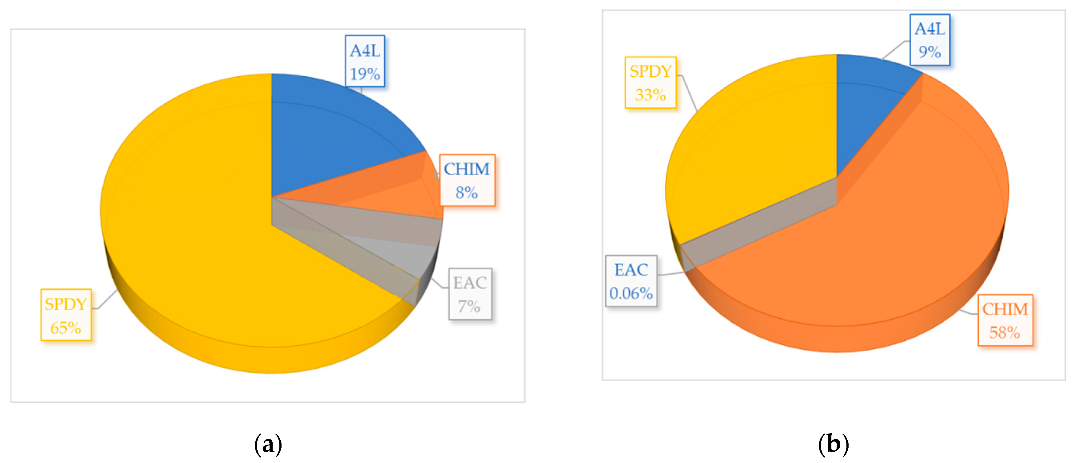
Figure 2.
Assets’ shares in the optimal risk portfolio for 31.10.2022: (a) Portfolio, constructed using the ARIMA predictions; (b) Portfolio, constructed using the Modified ODE predictions.
Figure 2.
Assets’ shares in the optimal risk portfolio for 31.10.2022: (a) Portfolio, constructed using the ARIMA predictions; (b) Portfolio, constructed using the Modified ODE predictions.
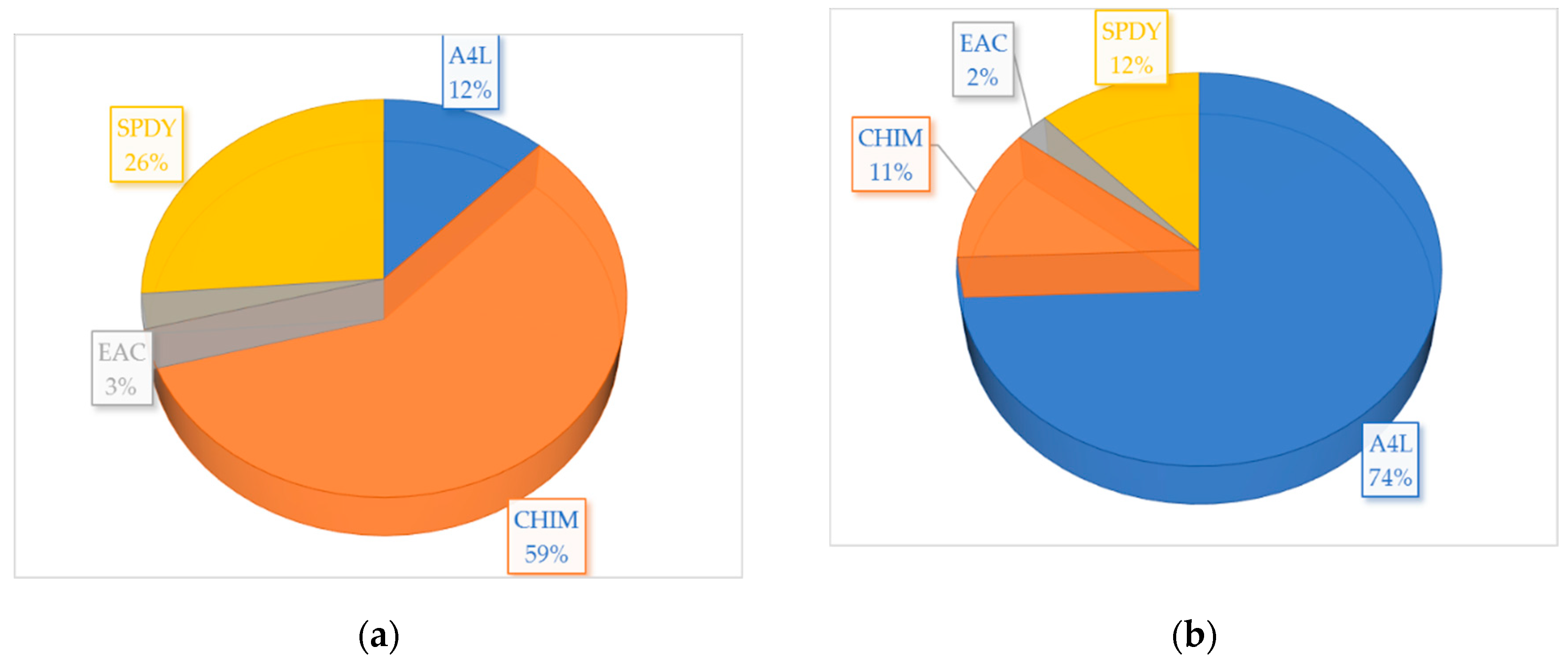

Table 1.
Financial results of the four companies to the end of 2020.
| Company | Market Capital (million BGN) | Turnover for the previous year (BGN) | Total Assets (pieces) |
Price per share (BGN) |
|---|---|---|---|---|
| Alterco JSC. | 194.400 | 11 617 459.00 | 17 999 999 | 6.77 |
| Elana AgroCredit JSC | 38.828 | 3 114 040.94 | 36 629 925 | 1.02 |
| Speedy JSC | 408.699 | 2 884 193.70 | 5 377 619 | 58.39 |
| Chimimport JSC | 225.267 | 9 080 952.02 | 239 646 267 | 0.94 |
Table 2.
Financial results of the four companies to the end of 2022.
| Company | Market Capital (million BGN) | Turnover for the previous year (BGN) | Total Assets (pieces) |
Price per share (BGN) |
|---|---|---|---|---|
| Alterco JSC. | 743 698 934 | 20 757 003 | 17 999 999 | 41.20 |
| Elana AgroCredit JSC | 37 362 524 | 193 821 | 36 629 925 | 0.95 |
| Speedy JSC | 548 517 138 | 52 109 | 5 377 619 | 97.18 |
| Chimimport JSC | 189 320 551 | 540 312 | 239 646 267 | 0.79 |
Table 3.
Absolute errors of the predictions of the closing prices of A4L instrument under different model selection.
Table 3.
Absolute errors of the predictions of the closing prices of A4L instrument under different model selection.
| Error | l=142 | l=143 | l=144 | l=147 | l=148 | l=149 |
|---|---|---|---|---|---|---|
| ARIMA (2, 1, 6) | 0.04 | 0.18 | 0.07 | 0.04 | 0.10 | 0.14 |
| ARIMA (1, 0, 10) | 0.08 | 0.10 | 0.01 | 0.25 | 0.07 | 0.08 |
Table 4.
Absolute errors of the predictions of the closing prices of CHIM instrument under different model selection.
Table 4.
Absolute errors of the predictions of the closing prices of CHIM instrument under different model selection.
| Error | l=142 | l=143 | l=147 | l=148 | l=149 | l=150 |
|---|---|---|---|---|---|---|
| ARIMA (4, 1, 7) | 0.01 | 0.01 | 0.01 | 0.04 | 0.01 | 0.01 |
| ARIMA (3, 1, 10) | 0.01 | 0.01 | 0.01 | 0.03 | 0.01 | 0.01 |
Table 5.
Absolute errors of the predictions of the closing prices of EAC instrument under different model selection.
Table 5.
Absolute errors of the predictions of the closing prices of EAC instrument under different model selection.
| Error | l=142 | l=143 | l=144 | l=148 | l=149 | l=150 |
|---|---|---|---|---|---|---|
| ARIMA (2, 1, 6) | 0.01 | 0.00 | 0.02 | 0.01 | 0.01 | 0.01 |
| ARIMA (1, 0, 6) | 0.00 | 0.01 | 0.01 | 0.00 | 0.00 | 0.00 |
Table 6.
Absolute errors of the predictions of the closing prices of SPDY instrument under different model selection.
Table 6.
Absolute errors of the predictions of the closing prices of SPDY instrument under different model selection.
| Error | l=143 | l=144 | l=147 | l=148 | l=149 | l=150 |
|---|---|---|---|---|---|---|
| ARIMA (2, 1, 9) | 1.17 | 0.38 | 0.06 | 0.62 | 0.33 | 0.66 |
| ARIMA (3, 1, 10) | 1.02 | 0.26 | 0.21 | 0.80 | 0.37 | 0.93 |
Table 7.
Predicted value and weighted average error on the chosen models.
| Instrument | Model | Predicted Value 30.10.2020 | Weighted Average Error |
| A4L | ARIMA (2, 1, 6) | 5.1525 | 0.0965 |
| ARIMA (1, 0, 10) | 5.0102 | 0.0993 | |
| CHIM | ARIMA (4, 1, 7) | 0.8826 | 0.0152 |
| ARIMA (3, 1, 10) | 0.8758 | 0.0135 | |
| EAC | ARIMA (2, 1, 6) | 1.0477 | 0.0101 |
| ARIMA (1, 0, 6) | 1.0394 | 0.0031 | |
| SPDY | ARIMA (2, 1, 9) | 56.3522 | 0.5224 |
| ARIMA (3, 1, 10) | 56.0732 | 0.6015 |
Table 8.
Predicted price values, actual price values, and relative error in % between them, using ARIMA models.
Table 8.
Predicted price values, actual price values, and relative error in % between them, using ARIMA models.
| Financial Instrument | Estimated Value for 30.10.2020 | Actual Value for 30.10.2020 | Relative Error in % |
|---|---|---|---|
| A4L | 5.0824 | 4.98 | 2.0562 |
| CHIM | 0.8790 | 0.87 | 1.0343 |
| EAC | 1.0413 | 1.04 | 0.1297 |
| SPDY | 56.2225 | 57.00 | 1.3640 |
Table 9.
Estimated values of the closing prices of A4L instrument for 30.10.2020 under different model selection.
Table 9.
Estimated values of the closing prices of A4L instrument for 30.10.2020 under different model selection.
| N=2 | N=3 | N=4 | N=5 | |
|---|---|---|---|---|
| M=0 | 4.90745529 | 4.98598555 | 4.95327385 | 4.96481506 |
| M=1 | 4.97275028 | 5.01424806 | 4.96156056 | 4.98925774 |
| M=2 | 4.99511213 | 5.00484627 | 4.99079255 | 4.99359350 |
| M=3 | 4.97263563 | 4.97089067 | 4.98461649 | 5.03006978 |
Table 10.
“Final errors” in the “test values” for the closing price of the A4L instrument for 30.10.2020 under different model choices.
Table 10.
“Final errors” in the “test values” for the closing price of the A4L instrument for 30.10.2020 under different model choices.
| N=2 | N=3 | N=4 | N=5 | |
|---|---|---|---|---|
| M=0 | 0.18932300 | 0.08999000 | 0.10401000 | 0.09520800 |
| M=1 | 0.06219800 | 0.06042200 | 0.07046000 | 0.05216000 |
| M=2 | 0.05609000 | 0.05729700 | 0.07161400 | 0.06046400 |
| M=3 | 0.05329500 | 0.04844100 | 0.05475100 | 0.08019361 |
Table 11.
Estimated values of the closing prices of CHIM instrument for 30.10.2020 under different model selection.
Table 11.
Estimated values of the closing prices of CHIM instrument for 30.10.2020 under different model selection.
| N=2 | N=3 | N=4 | N=5 | |
|---|---|---|---|---|
| M=0 | 0.87489373 | 0.87429690 | 0.87534827 | 0.87531741 |
| M=1 | 0.87412298 | 0.87589180 | 0.87690157 | 0.87555787 |
| M=2 | 0.87766096 | 0.87413580 | 0.87592214 | 0.87634988 |
| M=3 | 0.87502000 | 0.86701128 | 0.88030389 | 0.87573981 |
Table 12.
“Final errors” in the “test values” for the closing price of the CHIM instrument for 30.10.2020 under different model choices.
Table 12.
“Final errors” in the “test values” for the closing price of the CHIM instrument for 30.10.2020 under different model choices.
| N=2 | N=3 | N=4 | N=5 | |
|---|---|---|---|---|
| M=0 | 0.01420000 | 0.01400000 | 0.01420000 | 0.01430000 |
| M=1 | 0.01330000 | 0.01400000 | 0.01980000 | 0.01560000 |
| M=2 | 0.01340000 | 0.01490000 | 0.01340000 | 0.01540000 |
| M=3 | 0.01510000 | 0.01380000 | 0.01500000 | 0.01560000 |
Table 13.
Estimated values of the closing prices of EAC instrument for 30.10.2020 under different model selection.
Table 13.
Estimated values of the closing prices of EAC instrument for 30.10.2020 under different model selection.
| N=2 | N=3 | N=4 | N=5 | |
|---|---|---|---|---|
| M=0 | 1.04212540 | 1.04189833 | 1.04209529 | 1.04212314 |
| M=1 | 1.03991230 | 1.03980694 | 1.03805716 | 1.03904323 |
| M=2 | 1.04048472 | 1.03967983 | 1.03889503 | 1.03924009 |
| M=3 | 1.04181828 | 1.03898386 | 1.03758105 | 1.04532655 |
Table 14.
“Final errors” in the “test values” for the closing price of the EAC instrument for 30.10.2020 under different model choices.
Table 14.
“Final errors” in the “test values” for the closing price of the EAC instrument for 30.10.2020 under different model choices.
| N=2 | N=3 | N=4 | N=5 | |
|---|---|---|---|---|
| M=0 | 0.00430000 | 0.00430000 | 0.00420000 | 0.00440000 |
| M=1 | 0.00340000 | 0.00330000 | 0.00330000 | 0.00340000 |
| M=2 | 0.00370000 | 0.00400000 | 0.00330000 | 0.00380000 |
| M=3 | 0.00340000 | 0.00430000 | 0.00480000 | 0.00380000 |
Table 15.
Estimated values of the closing prices of SPDY instrument for 30.10.2020 under different model selection.
Table 15.
Estimated values of the closing prices of SPDY instrument for 30.10.2020 under different model selection.
| N=2 | N=3 | N=4 | N=5 | |
|---|---|---|---|---|
| M=0 | 56.98555970 | 57.00013130 | 57.04942020 | 57.03924550 |
| M=1 | 56.74659640 | 57.42282660 | 57.42797470 | 57.39400600 |
| M=2 | 57.36807520 | 57.39498800 | 57.53083620 | 57.08794140 |
| M=3 | 56.20392870 | 56.22095520 | 56.95981960 | 58.03724570 |
Table 16.
“Final errors” in the “test values” for the closing price of the SPDY instrument for 30.10.2020 under different model choices.
Table 16.
“Final errors” in the “test values” for the closing price of the SPDY instrument for 30.10.2020 under different model choices.
| N=2 | N=3 | N=4 | N=5 | |
|---|---|---|---|---|
| M=0 | 0.80750000 | 0.93660000 | 0.81690000 | 0.95910000 |
| M=1 | 0.97150000 | 0.89980000 | 0.99540000 | 0.95690000 |
| M=2 | 0.99070000 | 1.18890000 | 1.09240000 | 0.91740000 |
| M=3 | 0.99830000 | 0.89910000 | 1.21720000 | 0.96360000 |
Table 17.
Predicted price values, actual price values, and relative error in % between them, using Modified ODE models.
Table 17.
Predicted price values, actual price values, and relative error in % between them, using Modified ODE models.
| Financial Instrument | Estimated Value for 30.10.2020 | Actual Value for 30.10.2020 | Relative Error in % |
|---|---|---|---|
| A4L | 4.9846 | 4.98 | 0.0921 |
| CHIM | 0.8752 | 0.87 | 0.5998 |
| EAC | 1.0404 | 1.04 | 0.0382 |
| SPDY | 57.1085 | 57.00 | 0.1902 |
Table 18.
Absolute errors of the predictions from the ARIMA models, applied to the data for 2022.
| Instrument | ARIMA (p, d, q) | Absolute Errors | |||||
|---|---|---|---|---|---|---|---|
| l=142 | l=145 | l=146 | l=147 | l=148 | l=149 | ||
| A4L | (2, 1, 6) | 0.1048 | 0.1420 | 0.0532 | 0.6884 | 0.4907 | 0.1009 |
| (1, 0, 10) | 0.0397 | 0.0483 | 0.2304 | 0.6647 | 0.5802 | 0.1506 | |
| CHIM | (4, 1, 7) | 0.0186 | 0.0089 | 0.0302 | 0.0100 | 0.0128 | 0.0050 |
| (3, 1, 10) | 0.0031 | 0.0014 | 0.0354 | 0.0086 | 0.0269 | 0.0122 | |
| EAC | (2, 1, 6) | 0.0196 | 0.0013 | 0.0059 | 0.0191 | 0.0114 | 0.0024 |
| (1, 0, 6) | 0.0229 | 0.0153 | 0.0219 | 0.0198 | 0.0198 | 0.0224 | |
| SPDY | (2, 1, 9) | 3.5699 | 1.1275 | 0.2297 | 0.6225 | 0.4253 | 0.6345 |
| (3, 1, 10) | 4.3457 | 0.7079 | 0.2853 | 0.2296 | 1.2233 | 0.4009 | |
Table 19.
Predicted value and weighted average error on the chosen models.
| Instrument | Model | Predicted Value for 31.10.2022 | Weighted Average Error |
| A4L | ARIMA (2, 1, 6) | 17.6247 | 0.2744 |
| ARIMA (1, 0, 10) | 17.8545 | 0.3029 | |
| CHIM | ARIMA (4, 1, 7) | 0.7786 | 0.0137 |
| ARIMA (3, 1, 10) | 0.7804 | 0.0152 | |
| EAC | ARIMA (2, 1, 6) | 0.9789 | 0.0097 |
| ARIMA (1, 0, 6) | 1.0144 | 0.0204 | |
| SPDY | ARIMA (2, 1, 9) | 107.6251 | 0.9923 |
| ARIMA (3, 1, 10) | 107.5661 | 1.0772 |
Table 20.
Predicted price values, actual price values, and relative error in % between them, using ARIMA models.
Table 20.
Predicted price values, actual price values, and relative error in % between them, using ARIMA models.
| Financial Instrument | Estimated Value for 31.10.2022 | Actual Value for 31.10.2022 | Relative Error in % |
|---|---|---|---|
| A4L | 17.7339 | 18.65 | 4.9119 |
| CHIM | 0.7795 | 0.78 | 0.0701 |
| EAC | 0.9903 | 0.995 | 0.4714 |
| SPDY | 107.5968 | 107.00 | 0.5578 |
Table 21.
Estimated values of the closing prices of A4L instrument for 31.10.2022 under different model selection.
Table 21.
Estimated values of the closing prices of A4L instrument for 31.10.2022 under different model selection.
| N=2 | N=3 | N=4 | N=5 | |
|---|---|---|---|---|
| M=0 | 18.28096355 | 18.09513597 | 18.08016462 | 17.89179719 |
| M=1 | 18.17829696 | 18.00695886 | 18.01112314 | 18.05661753 |
| M=2 | 19.66848655 | 19.15769258 | 18.72543461 | 16.97272997 |
| M=3 | 16.91553048 | 18.70972867 | 16.12132696 | 21.36109005 |
Table 22.
“Final errors” in the “test values” for the closing price of the A4L instrument for 31.10.2022 under different model choices.
Table 22.
“Final errors” in the “test values” for the closing price of the A4L instrument for 31.10.2022 under different model choices.
| N=2 | N=3 | N=4 | N=5 | |
|---|---|---|---|---|
| M=0 | 0.10055900 | 0.07681535 | 0.08236390 | 0.04989364 |
| M=1 | 0.15965715 | 0.08840078 | 0.07980459 | 0.08133888 |
| M=2 | 0.01886979 | 0.05639571 | 0.05568973 | 0.00743097 |
| M=3 | 0.07079675 | 0.03217803 | 0.03329889 | 0.00650684 |
Table 23.
Estimated values of the closing prices of CHIM instrument for 31.10.2022 under different model selection.
Table 23.
Estimated values of the closing prices of CHIM instrument for 31.10.2022 under different model selection.
| N=2 | N=3 | N=4 | N=5 | |
|---|---|---|---|---|
| M=0 | 0.80500336 | 0.78203687 | 0.79825092 | 0.78912960 |
| M=1 | 0.79096175 | 0.79034851 | 0.79107247 | 0.79014385 |
| M=2 | 0.77761242 | 0.77231375 | 0.76321097 | 0.81030482 |
| M=3 | 0.79378890 | 0.77494780 | 0.82276553 | 0.78763064 |
Table 24.
“Final errors” in the “test values” for the closing price of the CHIM instrument for 31.10.2022 under different model choices.
Table 24.
“Final errors” in the “test values” for the closing price of the CHIM instrument for 31.10.2022 under different model choices.
| N=2 | N=3 | N=4 | N=5 | |
|---|---|---|---|---|
| M=0 | 0.03933323 | 0.05206715 | 0.03723752 | 0.07488105 |
| M=1 | 0.10632697 | 0.10693371 | 0.10709779 | 0.10159614 |
| M=2 | 0.03494464 | 0.05875035 | 0.03669832 | 0.03072809 |
| M=3 | 0.05611642 | 0.06096068 | 0.01475785 | 0.08157008 |
Table 25.
Estimated values of the closing prices of EAC instrument for 31.10.2022 under different model selection.
Table 25.
Estimated values of the closing prices of EAC instrument for 31.10.2022 under different model selection.
| N=2 | N=3 | N=4 | N=5 | |
|---|---|---|---|---|
| M=0 | 0.97349605 | 1.05003867 | 0.98470937 | 0.99199108 |
| M=1 | 0.99967003 | 0.99980277 | 0.99943251 | 1.00033667 |
| M=2 | 1.00902475 | 0.98998030 | 0.97504687 | 1.0045637 |
| M=3 | 1.03042746 | 0.99630033 | 0.97227905 | 0.9887555 |
Table 26.
“Final errors” in the “test values” for the closing price of the EAC instrument for 31.10.2022 under different model choices.
Table 26.
“Final errors” in the “test values” for the closing price of the EAC instrument for 31.10.2022 under different model choices.
| N=2 | N=3 | N=4 | N=5 | |
|---|---|---|---|---|
| M=0 | 0.02386445 | 0.01023558 | 0.10329024 | 0.01240245 |
| M=1 | 0.10902632 | 0.13969440 | 0.13510329 | 0.12584670 |
| M=2 | 0.02729210 | 0.05297982 | 0.06652198 | 0.06267512 |
| M=3 | 0.03251327 | 0.02605377 | 0.03249936 | 0.04000114 |
Table 27.
Estimated values of the closing prices of SPDY instrument for 31.10.2022 under different model selection.
Table 27.
Estimated values of the closing prices of SPDY instrument for 31.10.2022 under different model selection.
| N=2 | N=3 | N=4 | N=5 | |
|---|---|---|---|---|
| M=0 | 106.82119691 | 110.10191152 | 107.37708304 | 106.83075939 |
| M=1 | 106.89208241 | 106.82065168 | 107.02550172 | 106.91839134 |
| M=2 | 100.89401340 | 97.422710508 | 112.29010460 | 102.64214538 |
| M=3 | 95.362169097 | 89.974116039 | 119.80544693 | 107.98492701 |
Table 28.
“Final errors” in the “test values” for the closing price of the SPDY instrument for 31.10.2022 under different model choices.
Table 28.
“Final errors” in the “test values” for the closing price of the SPDY instrument for 31.10.2022 under different model choices.
| N=2 | N=3 | N=4 | N=5 | |
|---|---|---|---|---|
| M=0 | 0.09308016 | 0.09909670 | 0.09640184 | 0.08576109 |
| M=1 | 0.09448638 | 0.10674863 | 0.09032125 | 0.08246354 |
| M=2 | 0.03791003 | 0.02761275 | 0.04940139 | 0.06708805 |
| M=3 | 0.00618474 | 0.00493533 | 0.01082146 | 0.04768667 |
Table 29.
Predicted price values, actual price values, and relative error in % between them, using Modified ODE models.
Table 29.
Predicted price values, actual price values, and relative error in % between them, using Modified ODE models.
| Financial Instrument | Estimated Value for 31.10.2022 | Actual Value for 31.10.2022 | Relative Error in % |
|---|---|---|---|
| A4L | 18.1758 | 18.65 | 2.5426 |
| CHIM | 0.7899 | 0.78 | 1.2692 |
| EAC | 0.9998 | 0.995 | 0.4824 |
| SPDY | 106.6469 | 107.00 | 0.3300 |
Table 30.
Expected Rates of Return and Standard Deviations.
| Financial Instrument | Expected RoR – ARIMA 2020 | Expected RoR – Modified ODE 2020 | Std. Deviation 2020 | Expected RoR – ARIMA 2022 | Expected RoR – Modified ODE 2022 | Std. Deviation 2022 |
|---|---|---|---|---|---|---|
| A4L | 1.6480% | -0.31% | 3.3276% | 0.1917% | 2.6881% | 2.1724% |
| CHIM | -0.1136% | -0.54% | 1.7765% | -1.0846% | 0.2411% | 1.9702% |
| EAC | 0.1250% | 0.04% | 1.2198% | -0.4714% | 0.4824% | 7.1714% |
| SPDY | -1.3640% | 0.19% | 1.5851% | 0.5578% | -0.3300% | 1.9739% |
Table 31.
Correlation matrix for 2020.
| Financial Instrument | A4L | CHIM | EAC | SPDY |
| A4L | 1.0000 | 0.0430 | 0.0572 | -0.1008 |
| CHIM | 0.0430 | 1.0000 | 0.0820 | -0.1137 |
| EAC | 0.0572 | 0.0820 | 1.0000 | -0.0294 |
| SPDY | -0.1008 | -0.1137 | -0.0294 | 1.0000 |
Table 32.
Correlation matrix for 2022.
| Financial Instrument | A4L | CHIM | EAC | SPDY |
| A4L | 1.0000 | -0.0523 | -0.0444 | -0.0255 |
| CHIM | -0.0523 | 1.0000 | -0.0246 | 0.0880 |
| EAC | -0.0444 | -0.0246 | 1.0000 | -0.0476 |
| SPDY | -0.0255 | 0.0880 | -0.0476 | 1.0000 |
Table 33.
Predictions, actual values, and relative error in % between predicted and actual closing price values for different instruments for 30.10.2020 and 31.10.2022.
Table 33.
Predictions, actual values, and relative error in % between predicted and actual closing price values for different instruments for 30.10.2020 and 31.10.2022.
| Financial Instrument | Date | Estimated Value ARIMA | Portfolio Weights ARIMA % | Estimated Value ODE | Portfolio Weights ODE % | Last Known Price | Actual Price |
| A4L | 30.10.2020 | 5.0824 | 19.23 (+) | 4.9846 | 9.18 (-) | 5.00 | 4.98 (-) |
| 31.10.2022 | 17.7339 | 12.10 (+) | 18.1758 | 74.41 (+) | 17.70 | 18.65 (+) | |
| CHIM | 30.10.2020 | 0.8790 | 8.37 (-) | 0.8752 | 57.77 (-) | 0.88 | 0.87 (-) |
| 31.10.2022 | 0.7795 | 58.86 (-) | 0.7899 | 11.12 (+) | 0.79 | 0.78 (-) | |
| EAC | 30.10.2020 | 1.0413 | 7.20 (+) | 1.0404 | 0.06 (+) | 1.04 | 1.04 (0) |
| 31.10.2022 | 0.9903 | 2.85 (-) | 0.9998 | 2.42 (+) | 1.00 | 0.995 (-) | |
| SPDY | 30.10.2020 | 56.2225 | 65.21 (-) | 57.1085 | 32.99 (+) | 57.00 | 57.00 (0) |
| 31.10.2022 | 107.5968 | 26.18 (+) | 106.6469 | 12.05 (-) | 107.00 | 107.00 (0) |
Table 34.
Expected Rates of Return, Standard Deviations, and Real Percentage Return of the Optimal Risk Portfolio.
Table 34.
Expected Rates of Return, Standard Deviations, and Real Percentage Return of the Optimal Risk Portfolio.
| Method used for the predictions | Date | Expected RoR of the Risk Portfolio | Standard Deviation Estimate of the Risk Portfolio | Real Percentage Return |
|---|---|---|---|---|
| ARIMA | 30.10.2020 | 1.2248% | 1.1622% | 0.0190% |
| 31.10.2022 | 0.8211% | 1.3278% | 1.3853% | |
| ODE | 30.10.2020 | 0.4031% | 1.1371% | 0.7009% |
| 31.10.2022 | 2.0784% | 1.6338% | 3.6356% |
Disclaimer/Publisher’s Note: The statements, opinions and data contained in all publications are solely those of the individual author(s) and contributor(s) and not of MDPI and/or the editor(s). MDPI and/or the editor(s) disclaim responsibility for any injury to people or property resulting from any ideas, methods, instructions or products referred to in the content. |
© 2023 by the authors. Licensee MDPI, Basel, Switzerland. This article is an open access article distributed under the terms and conditions of the Creative Commons Attribution (CC BY) license (http://creativecommons.org/licenses/by/4.0/).
Copyright: This open access article is published under a Creative Commons CC BY 4.0 license, which permit the free download, distribution, and reuse, provided that the author and preprint are cited in any reuse.


