
Submitted:
24 October 2023
Posted:
25 October 2023
You are already at the latest version
Abstract
Track fasteners play a pivotal role in infrastructure inspection for high-speed rail. Yet, images taken by drones often capture shadows cast by electrical towers flanking the high-speed rail tracks. These shadows can hinder the visibility of the track fasteners, thereby impacting detection efficiency and accuracy considerably. The present paper introduces an end-to-end shadow removal algorithm, rooted in generative adversarial network training. The comprehensive network framework is segmented into three sub-networks: pseudo-mask generation, shadow removal, and result refinement. We have integrated a Fourier convolutional residual module to bolster the feature extraction capability of the generator network. This integration ensures the network retains a global receptive field, even in its more superficial layers. By employing an overall weighted loss function, we enhance the quality of the images produced without shadows. Further, a perceptual loss function has been incorporated to retain the structural information of objects, setting the stage for subsequent defect detection. Our results highlight that Pse-ShadowNet adeptly eradicates fastener shadows while maintaining vital visual features, including object position, structure, texture, edges, and other key visual elements. Consequently, the reconstructed images are detailed and showcase superior image quality.
Keywords:
ballastless track
; image shadow removal
; generative adversarial network
; computer vision
1. Introduction
Ballastless tracks are predominant in China's high-speed railway network due to their benefits such as high smoothness, stability, durability, and ease of maintenance [1]. Indeed, they constitute the primary track structure for the Chinese high-speed railways. Ensuring the ballastless track's optimal operational condition is vital for the uninterrupted and safe movement of high-speed trains. Consequently, monitoring the track's condition and identifying any defects in its components are of paramount importance. In recent times, drone inspections have gained prominence in various sectors, including power equipment and road bridges, owing to their high efficiency, flexibility, and cost-effectiveness. When applied to railway inspection, drones can cover vast distances uninhibited by challenging terrains. They significantly reduce the interference with maintenance schedules, cut down on manpower and material expenses, enhance the efficiency of inspections, and broaden the scope of coverage.
During the image collection process using drones, shadows can manifest on the images, resulting from the fasteners' structure and drone inspection angles. These shadows often mask essential details, such as the contours and textures of the fasteners. For effective detection of missing fasteners later on, it's imperative to eliminate these shadows from the drone-captured images. Historically, shadow removal techniques predominantly banked on constructing physical models rooted in lighting and color information. These strategies pinpointed and eradicated shadows by designing features based on manual labeling of physical attributes, like color and lighting. Often, they were anchored in certain presuppositions, like assuming uniform lighting within shadowed regions [2]. A significant limitation of many such techniques was their capability to only dispel hard shadows, leaving soft shadows unaddressed. Some conventional algorithms also leveraged shadow edges for shadow removal. For instance, Finlayson et al. [3] utilized shadow edges to discern a scaling factor that distinguished between shadowed and non-shadowed regions, accomplishing shadow detection. Similarly, Wu et al. [4] identified pronounced shadow edges to obliterate shadows throughout the image. Shor and Lischinki [5] calculated affine transformation parameters contrasting shadowed and non-shadowed pixels, subsequently employing a pyramid restoration technique to produce shadow-less images. There were also methodologies necessitating user engagement. Gryka et al. [6] designed a regression model to comprehend the relationship between shadowed image zones and their corresponding shadow masks for autonomous shadow elimination. Nonetheless, this algorithm called for users to demarcate the regions demanding processing.
With the cascade of advancements in deep learning within image processing and computer vision, the research paradigm has gravitated towards deep learning-infused shadow removal techniques. As an illustration, Qu et al. [7] unveiled DeShadowNet, a tool that derives multi-scale contextual semantic information from diverse feature layers to forecast and curate shadow-free images. They also introduced a substantial SRD dataset. Many deep learning algorithms referenced earlier employ a supervised learning approach, necessitating training on paired shadow and shadow-free datasets. However, due to ever-changing natural lighting conditions, acquiring entirely paired datasets is inherently challenging in real-world scenarios. To counteract the reliance on these paired datasets, Hu et al. introduced Mask-ShadowGAN, grounded in the CycleGAN framework [8,9].This approach leverages unpaired datasets to train the network in shadow removal and employs generated binary masks to guide the network's learning process. A significant limitation, however, is the substantial domain disparity between the shadowed and shadow-free images within the training dataset. This gap means the algorithm struggles to accurately discern the relationship between shadowed and shadow-free domains, leading to subpar shadow-free image outputs. To address this, Liu et al. [10] put forth LG-ShadowNet, which employs brightness features to navigate the model in shadow removal. Jin et al. [11] then proposed DC-ShadowNet, an unsupervised learning network. Here, a domain classifier discerns between shadowed and shadow-free regions, directing the network to prioritize shadow regions. Additionally, they incorporated a suite of loss functions grounded in physical attributes to instruct the GAN network's training. Hieu and Dimitris [12] took a different route by training their model using shadowed and non-shadowed segments extracted from shadow images. Their algorithm is firmly anchored in strict physical constraints. Drawing inspiration from this, Liu et al. [13] devised G2R-ShadowNet. This model produces pseudo-shadows on cropped shadow-free zones and aligns them with their shadow-free counterparts. As a result, it embodies weakly supervised learning and delivers enhanced performance.
A significant portion of shadow removal algorithms grounded in deep learning relies on the adversarial training framework of the Generative Adversarial Network (GAN). However, the field has seen varied algorithmic studies beyond this approach. For instance, Cun et al. [14] introduced the Dual Hierarchical Aggregation Network (DHAN). This model employs a chain of incrementally expanding dilated convolutions as its central network, hierarchically aggregating multi-scale semantic features to predict and generate shadow-free images. Additionally, they developed the SMGAN network, aimed at producing shadow images to both augment the dataset and bolster model training. Fu et al. [15], on the other hand, devised an algorithm that initially overexposes the input image, making shadowed regions align in color characteristics with shadow-free zones. The method then merges the original and the overexposed images to render the final shadow-free image.
Employing deep learning to erase shadows from images not only bypasses intricate physical modeling and manual feature extraction but also enhances precision and adaptability across various environments and scenes. Nevertheless, a common limitation is that most algorithms necessitate fully paired shadow and shadow-free datasets. This becomes challenging, especially when sourcing images from drones for inspection purposes. To circumvent this challenge, the present paper puts forth an end-to-end shadow removal algorithm anchored in an unsupervised Generative Adversarial Network (GAN). The research delves into several facets, including the design of the network framework, the formulation of the loss function, and a comparative analysis of experimental outcomes.
Addressing the persistent challenge of shadows in drone-captured fastener images, this paper presents several novel contributions, detailed as follows:
- We present a shadow removal approach grounded in unsupervised generative adversarial training.
- Our detailed architectural design addresses the challenges drones encounter in capturing shadow-free images of fasteners in real-world scenarios.
- By leveraging a custom-designed loss function, our network optimizes the quality of images restored after shadow removal.
- Through rigorous comparative and ablation tests, we validate the robustness of our algorithm, laying a foundation for future studies on identifying absent rail fasteners.
The paper is organized into subsequent sections: Section 2 delves into the foundational principles of the Generative Adversarial Network (GAN) employed herein and elaborates on the dataset construction for experiments. Section 3 focuses on the design intricacies of the shadow removal network. Section 4 details the experimental methodology and findings, while Section 5 offers conclusive remarks.
2. Materials and Methods
2.1. Generative Adversarial Network
Machine learning can be divided into two learning modes: supervised learning and unsupervised learning, depending on whether the training dataset has labels. In supervised learning, a large dataset with labeled (ground truth) data is used to train the model. On the other hand, unsupervised learning does not require explicit labels and allows the algorithm to learn from its own mistakes, continuously improving the accuracy of predictions. Although supervised learning models can achieve high accuracy, the core issue lies in the need for extensive data annotation, which is time-consuming and labor-intensive. This highlights the superiority of unsupervised learning. Generative adversarial networks (GANs) are one of the most promising methods in the field of unsupervised learning in recent years.
The Generative Adversarial Network (GAN) is a probabilistic generative network model proposed by Goodfellow et al. in 2014 [16], which has been a hot topic in the field of deep learning since its inception. GAN is not just a specific network model, but a framework for adversarial training based on game theory. It consists of two network models: the generator and the discriminator, which represent the two players in the game. The core idea of GAN is to generate high-quality data samples that are close to the real distribution through adversarial training between the two neural network models. The network structure is shown in Figure 1.
The generator takes random noise as input and generates a fake image, while the discriminator takes a real or fake image as input and outputs the probability that the image is real. The so-called game between the two refers to the generator learning through network training to generate images that are closer to the real distribution in order to "deceive" the discriminator, while the discriminator improves its discrimination ability through neural network learning and "penalizes" the generator through a loss function. The two iteratively engage in adversarial training until reaching a Nash equilibrium, where the generator can fit the real data distribution and the discriminator cannot distinguish between fake and real images. Both the generator and the discriminator reach the optimal solution as the two players in the game.
The loss function of the entire Generative Adversarial Network (GAN) is defined as follows:
In the equation, represents the real samples, represents the input random noise, represents the value returned by the discriminator when the sample data is input, represents the generated samples outputted by the generator when the noise is input, represents the distribution of real image data, and represents the distribution of generated image data.
Equation (1) is fundamentally a minimax optimization problem. Correspondingly, during the training process, a step-by-step optimization strategy is adopted, where discriminator D is optimized first by fixing the generator weights, and then generator G is optimized by fixing the discriminator weights. This process is repeated until convergence or reaching the maximum number of iterations. This adversarial training is not a traditional one-way iterative update, but rather a mutual influence between the two models. The gradient update parameters for the generator are obtained from the corresponding discriminator rather than the training data samples.
2.2. Dataset Construction
Currently, deep learning-based shadow removal methods for image processing generally utilize two types of datasets based on supervised and unsupervised learning modes.
In the supervised learning mode, paired datasets are used, with the representative dataset being ISTD. This dataset consists of 1870 sets of triplets, which include a shadow image, its corresponding mask, and an image without shadows as a set. The image size is .
In the unsupervised learning mode, unpaired datasets are used, with the representative dataset being USR. This dataset consists of randomly selected 2,445 shadow images and 1,770 images without shadows, without any corresponding relationship between them.
Due to the organizational structure and positioning issues of the fasteners, as well as the ever-changing natural environment, it is difficult to collect real shadow-free fastener images. In other words, there are no real labels to guide the model training. Therefore, the algorithm uses an unpaired dataset for unsupervised learning.
First, image collection is done using a camera mounted on a drone, with an image resolution of . Then, the image size is adjusted. If the original fastener image resolution is used for training, it will cause memory overflow, and the training time will be very long. In addition, the training of the generative adversarial network itself is very difficult. After balancing image quality and training efficiency, this study uses as the network input image size, referring to the ISTD dataset. Photoshop's slice processing is used, and parts containing fastener shadows are selected from it, as shown in Figure 2.
This paper uses Photoshop software to create the binary shadow mask images. First, batch processing in PS is used to binarize all resized fastener images, and then drawing tools such as rectangle and fill are used to restore the areas unrelated to the shadow to white. The rough edges of the shadow areas are finely marked. Finally, the Matlab software program is used to perform inverse binarization to obtain the final mask. The annotation process is shown in Figure 3.
3. Shadow Removal Network Pse-ShadowNet
This paper proposes an end-to-end shadow removal network called Pse-ShadowNet (Pseudo mask Shadow removal Network) based on unsupervised generative adversarial networks. The overall network architecture consists of three sub-networks: the pseudo mask generation sub-network, the shadow removal sub-network, and the result refinement sub-network. These three parts are jointly trained. The pseudo mask generation sub-network consists of a pseudo mask generator and a discriminator, while the result refinement sub-network consists of a result refinement module and a discriminator.
3.1. Design of Adversarial Training Network Framework
- (1)
- Pseudo mask generator
At the beginning of the algorithm, the construction of the dataset required as input for the pseudo mask generator follows the specific steps as outlined below: First, a specific shadow mask is selected from the training set, along with its corresponding shadow image . The shadow mask is then applied to the shadow region of , resulting in the extraction of the corresponding shadow area . The remaining pixels in the image are automatically set to 0. Next, another random shadow mask is selected from the training set and applied to the non-shadow region of , resulting in the creation of a non-shadow region . The area of is approximately similar to that of the shadow region , subject to the constraint:
Where the operation is responsible for calculating the area of the given region, in this paper's experiments, is set to 0.2.
As shown in Figure 4, through the aforementioned operations, non-paired training data is constructed, consisting of the shadow region and the non-shadow region .
After obtaining this training data, the non-shadow region is inputted into the pseudo mask generator, resulting in the output pseudo shadow image . In this adversarial training process, the first discriminator is introduced. The discriminator should classify the generated pseudo shadow as false, while the real shadow region should be classified as true. The discriminator, through a loss function penalty mechanism, helps train the pseudo mask generator to output shadow images that are closer to the real distribution. Additionally, inspired by the CycleGan network's cycle consistency loss function (identity loss), the shadow region is also fed into the pseudo mask generator to obtain the output . The content of both images should remain consistent, and this loss function further guides the training of the pseudo mask generator.
- (2)
- Shadow removal network
The role of the shadow removal network R is to remove the pseudo shadow generated by the pseudo mask generator. The output of the pseudo mask generator , when combined with , is used as input for the shadow removal network. The network then produces the non-shadow region . In theory, the content of should be identical to that of . The workflow of the shadow removal network is shown in Figure 5. In this training process, since and correspond to the shadow and non-shadow regions of the same content in the image, they can be considered as paired training data, establishing a weakly supervised learning mode.
- (3)
- Result refinement network
The output of the shadow removal network is embedded into the original input shadow image , resulting in the output . Then, is concatenated with , resulting in a rough output image . This image has 4 feature channels, including 3 channels from and 1 channel from the mask. However, the color of may not be perfectly consistent with the color of the original input image , leading to lower generated image quality. To address this, a result refinement network R is introduced to fully utilize the contextual semantic features of the original shadow image to remove shadows and enhance the quality of the reconstructed image, resulting in the final output non-shadow image . In this process, a second discriminator is introduced. The discriminator should classify the output from the result refinement network as fake while classifying the real original input image as real. The three subnetworks are unified into an overall adversarial training framework, as shown in Figure 6.
During the inference testing stage, the network will discard the two discriminators and the pseudo mask generator, leaving only the shadow removal network and the result refinement network in the entire network framework. By inputting the shadow image and its corresponding mask into the network, the corresponding non-shadow image can be outputted, achieving end-to-end image shadow removal. The process is shown in Figure 7.
In the entire joint training network framework, the pseudo mask generator, shadow removal network, and result refinement network all act as generators and adopt the same encoder-decoder network structure, as shown in Figure 8 (a). Firstly, three 3x3 convolutional layers with a stride of 2 are used for downsampling to reduce the resolution of the input image. The middle part is the feature extraction module of the network, as shown in Figure 8 (b). Finally, three transpose convolution operations are used for upsampling to restore the resolution and output the image.
In constructing the generator network structure, this paper utilizes residual modules based on Fourier convolution, which can be seen as a lightweight alternative to the self-attention mechanism. It enhances the feature extraction capability of the generator network and helps the network model generate visually high-quality images.
Fast Fourier Convolution (FFC) [17] is a convolution computation method based on channel-level Fast Fourier Transform (FFT). Its principle is to transform the convolution operation into point-wise multiplication in the frequency domain, greatly improving computational efficiency. It has been widely used in signal processing, image processing, speech recognition, and other fields. In computer vision tasks, Fourier convolution enables the network to have a global receptive field that spans the entire image even in shallow layers.
Traditional convolutional neural networks (CNNs) tend to capture basic visual features from the edges or contours of images. Therefore, it can be concluded that the original CNN-style convolutional residual modules may have good capabilities in learning high-frequency components but lack powerful representation ability in modeling low-frequency information.
In this paper, residual modules based on Fourier convolution are used as shown in Figure 8 (c). They can be divided into three branches. The local branch utilizes the original residual module and focuses on capturing local feature information in the image. The global branch, on the other hand, adopts a convolutional form based on a fast Fourier transform. With these two branches, the network can simultaneously capture both high-frequency and low-frequency features. Additionally, there is also an identity mapping branch.
Let the input feature vector be , where , , and represent the height, width, and channels of the feature volume. The calculation steps of the global branch using Fourier convolution in the Res FFT-Conv block are as follows:
- (1)
- Perform a 2D real FFT operation to obtain :
- (2)
- Concatenate the real and imaginary parts along the feature channel to obtain :
- (3)
- Apply a stack of two 1x1 convolutions with an intermediate ReLU layer to obtain :
- (4)
- Perform an inverse 2D real FFT operation to return to the spatial domain.
In the above equation, all frequency domains share the same weights, allowing for the capture and modeling of feature information across all frequency domains.
The final output of the Fourier Convolutional Residual Module is:
The calculation of is the same as the calculation of the original residual module.
The design of the local and global branches in the Fourier Convolutional Residual Module allows the generator network to capture both high-frequency and low-frequency information simultaneously. It also enables the learning of long-range spatial dependencies in the frequency domain, undoubtedly enhancing the feature extraction capability of the feature extraction module. This paper demonstrates that stacking only six Fourier Convolutional Residual Modules achieves excellent feature representation, reducing the depth of the generator network to a certain extent, which can help stabilize the training of the generative adversarial network.
Both discriminators adopt the same network structure based on PatchGAN [18], as shown in Figure 9. In the original GAN network, the discriminator outputs a scalar value representing whether the input is real or fake, providing discrimination for the entire image. However, the PatchGAN discriminator utilizes a fully convolutional network. During the discrimination process, it applies convolutional operations to the entire image. The output is an N × N matrix, where each element corresponds to a specific region of the image due to the receptive field mechanism of convolution. Finally, each element in the matrix is classified as real or fake, and the weighted average of these classifications is taken as the discriminator's output.
By discriminating each patch instead of the entire image, the network's ability to extract local feature information is enhanced, allowing the network to focus more on image details. Additionally, for images with significant feature differences, the weighted average approach can provide a more reasonable loss expression compared to the original discriminator. This approach can effectively integrate both local and global characteristics of the image.
3.2. Design of Overall Weighted Loss Function
In the training process of the generative adversarial network framework, there are multiple loss functions to quantify the performance of the generator and discriminator models. These loss functions provide guidance for training and can constrain the network to generate high-quality images as desired. In this section, we will introduce the loss functions used in the three subnets and the overall weighted loss function of the entire network framework.
- (1)
- Pseudo mask generation sub-network
When training the pseudo mask generation sub-network, we introduce loss functions for both the generator and the discriminator, defined as follows:
Therefore, the joint loss function for the entire sub-network adversarial training is:
In addition, to ensure that the pseudo mask generator can synthesize high-quality forged shadows, the real shadow region is inputted, and the same loss function (identical loss) is used to encourage the network to generate forged shadows that are as similar as possible to the input , defined as:
Whereas, , represents the L1 loss function.
- (2)
- Shadow removal sub-network
The loss function definition for training the shadow removal sub-network is as follows:
Because the output of the pseudo mask generator G is also the input to the shadow removal network R, the gradient computed by this loss will be backpropagated through to the pseudo mask generator G. Therefore, it can be considered as a cyclic loss function for jointly training G and R.
- (3)
- Result refinement sub-network
The loss function definition for training the result refinement sub-network is as follows:
The pixel-level loss function is calculated based on the semantic information of the entire original input shadow image, and its gradient will be backpropagated to both the pseudo mask generator G and the result refinement network R.
Most of the aforementioned loss functions are L1 loss functions, which may result in overly smooth or even blurry generated images. To address this issue and improve the reconstruction of structural and textural features in the shadow-removed images, this paper introduces a perceptual loss function [19]. Firstly, the generated image and the ground truth image are passed through a set of pre-trained convolutional neural networks to obtain feature vectors from multiple layers. Then, the error between these feature vectors is computed as the loss function, guiding the generator to generate more accurate and realistic images. The principle is illustrated in Figure 10.
Unlike the per-pixel loss function, the perceptual loss function utilizes multi-scale features extracted from a pre-trained loss network to quantify the visual and semantic differences between the generated and ground truth images. This helps train the network to generate images that are closer to the real distribution. In this paper, the pre-trained VGG16 [20] is used as the loss network, and features are extracted from the last layer of each of the first three stages (i.e., Conv1-2, Conv2-2, and Conv3-3). The perceptual loss is defined as follows:
Where represents the feature map expression of the three convolutional layers of VGG16 for (the generated shadow-free image) and (the ground truth shadow-free image). , ,and represent the dimensions of .
In the process of calculating the perceptual loss function, the interaction between the generator network and the discriminator network is taken into consideration, allowing the generator to better match the features and structures of real data samples during training. It can also address some issues that exist in traditional Generative Adversarial Networks (GANs), such as training instability, difficulty in distinguishing samples, and low quality of generated images.
The overall loss function of the entire network is as follows:
Where , , , , represent the weights of each loss function, and , , , , are set to 1.0, 5.0, 2.0, 1.0, 1.0 respectively.
4. Experimental Results and Analysis
In this paper, comparative experiments were conducted between Pse-ShadowNet and other deep learning-based shadow removal methods on public datasets and a drone fastener shadow dataset. The effectiveness of Pse-ShadowNet was evaluated quantitatively and qualitatively to demonstrate its performance. Additionally, details such as dataset descriptions, experimental setup, evaluation metrics, and training procedures were also provided.
4.1. Experimental Setup
- (1)
- Datasets
In this section of the experiment, the training dataset used consists of a combination of drone-captured fastener shadow images and the ISTD dataset. It includes two folders, test_A and test_B, as shown in Figure 11. The test_A folder contains the original images that require shadow removal, as shown in Figure 11 (a). The test_B folder contains the corresponding binary shadow masks, as shown in Figure 11 (b). The dataset consists of a total of 960 images, with 750 images used for training and 210 images used for testing. The images are uniformly resized to a size of 640 × 480 pixels.
- (2)
- Experimental environment
To better evaluate the performance of the shadow removal network architecture and loss function design, a series of environmental and experimental parameters will be configured before training. The specific settings are shown in Table 0.
- (3)
- Hyperparameter settings
In this chapter's experiment, random noise is used to initialize the parameters. The total number of iterations is set to 100 epochs. The generator learning rate is set to 1e-4, and the discriminator learning rate is set to 2e-4. The same learning rate is maintained for the first 50 training epochs, and then the learning rate linearly decays to 0 over the next 50 epochs until the end of training. The optimizer adopts Adam algorithm, the first momentum is set to 0.5 and the second is set to 0.999. Finally, considering the stability of training the generative adversarial network, the batch size during model training is set to 1.
- (4)
- Evaluation metrics
An effective shadow removal algorithm should not only remove shadow interference in the image but also ensure that the original shadow-free areas and overall visual effects in the image are not altered. This improves the quality of the generated image, including texture and edge information, while preserving more image structural features. This is crucial for subsequent defect detection in clipping. Therefore, in this paper, the root mean square error (RMSE), structural similarity index measure (SSIM), and peak signal-to-noise ratio (PSNR) are chosen as evaluation metrics for the algorithm.
- (1)
- RMSE
The root mean square error (RMSE) is defined as follows:
Among them, represents the ground truth shadow-free image, while represents the image generated after shadow removal by the algorithm. is the number of samples. A smaller value of RMSE indicates the better visual quality of the generated image.
- (2)
- SSIM
The structural similarity index measure (SSIM) is defined as follows:
Among them, and are two constants used for stabilization. represents the shadow-free image generated by the network, while represents the ground truth shadow-free image. and are the variances of and , and is the covariance between and . is the average pixel intensity of , and is the average pixel intensity of . The range of the structural similarity index measure (SSIM) is [0,1]. Similarly, a higher SSIM value indicates that the generated image is closer to the ground truth image.
RMSE simply calculates the pixel value differences between two images at corresponding positions. However, as a comprehensive image quality evaluation metric, SSIM comprehensively measures the similarity between two images in terms of brightness, contrast, and structure, thereby compensating for the limitations of the RMSE evaluation metric.
- (3)
- PSNR
The peak signal-to-noise ratio (PSNR) is defined as follows:
Among them, and represent the shadow-free image predicted by the model and the corresponding ground truth value, respectively. A higher PSNR value indicates better visual quality of the image generated by the network.
4.2. Comparative Analysis
We compared Pse-ShadowNet with other deep learning algorithms, such as Mask-ShadowGAN [21], CycleGAN [22]., LG-ShadowNet [23], and G2R-ShadowNet [24], on general dataset ISTD and fastener shadow dataset collected by drones.
- (1)
- Evaluation of the ISTD dataset
As shown in Figure 12, from the image we can see that all methods are capable of removing shadows from the original input image, especially in scenes with smaller shadow occlusion areas, where most algorithms can effectively remove shadows. However, there are slight differences in the quality of the generated images. Other algorithms may exhibit inconsistent colors with the surroundings at the transition edges of the shadows, which could result in more noticeable shadow boundaries. On the other hand, the shadow regions of the shadow-free images generated by Pse-ShadowNet exhibit more consistent colors with the surrounding areas, reflecting higher visual quality. Additionally, the algorithm achieves excellent reconstruction of image features in the shadow regions, such as the texture of the playground grass, the steps on the pavement, and the text on the bulletin board, providing a solid foundation for subsequent computer vision tasks such as accurate object detection and image classification. However, when the shadow coverage area is large, all types of shadow removal algorithms perform poorly, especially when the overall color distribution of the image is complex and the surrounding areas of the shadow are dark. In the process of reconstructing the shadow region, color distortion occurs. These algorithms fail to capture long-distance feature information and overly focus on local features, leading to the erroneous learning of dark features in the surrounding areas and the restoration in that region, resulting in the shadow region that should have been "brightened" remaining darker compared to the real image. Although the performance of the Pse-ShadowNet algorithm decreases in such large-scale shadow scenes, it still demonstrates good shadow removal effects in comparison to other algorithms, highlighting the robustness and generalization ability of the algorithm.
- (2)
- Evaluation of the fastener shadow dataset
As shown in Figure 13, all algorithms are capable of removing fastener shadows, but there are significant differences in the overall perception and local features of the generated images. The images generated by CycleGAN appear brighter overall compared to the original images, but the reconstruction and restoration of the fastener shadow regions are poor. The various visual features of the fasteners are not prominent, and there are numerous artifacts. LG-ShadowNet and Mask-ShadowGAN exhibit significant differences in color, brightness, and other physical features between the restored shadow regions and the surrounding areas. They also suffer from the issue of unclear fastener features. The fastener shadow regions generated by G2R-ShadowNet have a more natural transition with the surrounding areas, but the images generated are relatively smooth, resulting in the loss of corresponding structural features of the fasteners to some extent. Compared to other algorithms, Pse-ShadowNet effectively removes fastener shadows while preserving the visual features such as the position, structure, texture, and edges of the fasteners to a great extent. The reconstruction effects are clear, and the generated image quality is high, providing a solid data foundation for subsequent research on target detection algorithms focusing on fastener absence.
Due to the inability to collect shadow-free images corresponding to the shadow images during the process of collecting fastener image data with drones, this study only quantitatively evaluates the shadow removal performance of the designed Pse-ShadowNet on the general dataset ISTD, as shown in Table 0. Quantitative evaluation metrics are calculated separately for the shadow area, shadowless area, and the entire image to further demonstrate its shadow removal performance.

Table 2.
Quantitative comparison of results.
| model | Shadow area | Shadowless area | Entire image | ||||||
|---|---|---|---|---|---|---|---|---|---|
| RMSE | SSIM | PSNR | RMSE | SSIM | PSNR | RMSE | SSIM | PSNR | |
| Mask-ShadowGAN | 9.8 | 0.972 | 31.09 | 4.9 | 0.956 | 32.24 | 5.6 | 0.947 | 29.45 |
| CycleGAN | 10.8 | 0.968 | 31.56 | 9.3 | 0.961 | 28.17 | 9.7 | 0.934 | 28.55 |
| LG-ShadowNet | 9.8 | 0.982 | 32.45 | 3.7 | 0.975 | 33.73 | 4.3 | 0.947 | 29.22 |
| G2R | 9.3 | 0.979 | 34.02 | 2.4 | 0.983 | 36.21 | 3.6 | 0.952 | 31.54 |
| Our | 7.8 | 0.988 | 35.68 | 2.8 | 0.980 | 35.72 | 3.5 | 0.958 | 32.11 |
As shown in Figure 14 and Figure 15, it can be visually observed that the structural similarity index measure (SSIM) and peak signal-to-noise ratio (PSNR) of the shadow-free images generated by Pse-ShadowNet are higher than other deep learning-based shadow removal algorithms, indicating its effectiveness.
Figure 16 shows a visual comparison of the generated images with and without the perceptual loss function. In Figure 16 (a), the image generated without the perceptual loss function appears smoother, and the fastener features in the shadow region are not clearly noticeable. In Figure 16 (b), the image generated with the perceptual loss function shows better restoration of the fastener structure features.
5. Conclusions
In this study, we present an innovative image shadow removal method, termed Pse-ShadowNet, which is grounded on the principles of unsupervised generative adversarial network (GAN) training. This algorithm seamlessly produces shadow-less images through an end-to-end process. Pse-ShadowNet comprises three interlinked sub-networks: pseudo mask generation, shadow removal, and result refinement. These sub-networks incorporate three generators and two discriminators. During the generator network's design, we utilized an encoder-decoder architecture and incorporated residual modules rooted in Fourier convolution. Such a design accentuates the network's capability to identify shadow features, allowing the network to gain a comprehensive perspective at an initial stage. Consequently, there's a reduction in the network's layers, addressing the typical instability challenges associated with GAN training. The discriminator network, modeled after PatchGAN, emphasizes intricate image particulars, leading to images with more defined and crisper edges. Guided by the overarching weighted loss function, there's a noticeable enhancement in the visual quality of the images generated devoid of shadows. Notably, the inclusion of the perceptual loss function retains more structural data of fasteners, setting the stage for forthcoming fastener object detection methodologies.
Author Contributions
Conceptualization, X.F. and Z.Z.; methodology, Z.D.; validation, Z.W. and Y.J.; investigation, T.T.; writing—original draft, Z.D. All authors have read and agreed to the published version of the manuscript.
Funding
This work was supported by Beijing Municipal Science and Technology Project (No. Z181100003218013).
References
- Xu, J.; Wang, P.; An, B.; Ma, X.; Chen, R. Damage detection of ballastless railway tracks by the impact-echo method. In Proceedings of the Institution of Civil Engineers-Transport, Brisbane, Australia, 16-20 April 2018. [Google Scholar]
- Finlayson, G. D.; Hordley, S. D.; Lu, C. , Drew, M. S. On the removal of shadows from images. IEEE Transactions on Pattern Analysis and Machine Intelligence 2005, 28(1), 59–68. [Google Scholar]
- Finlayson, G. D.; Hordley, S. D.; Drew, M. S. Removing shadows from images. In Computer Vision—ECCV 2002: 7th European Conference on Computer Vision Copenhagen, Venezia, Italy, 30 October-3 November 200.
- Wu, Q.; Zhang, W.; & Kumar, B. V. Strong shadow removal via patch-based shadow edge detection. In 2012 IEEE International Conference on Robotics and Automation, Baden-Württemberg, Germany, 6-10 May 2012.
- Shor, Y.; Lischinski, D. The shadow meets the mask: Pyramid-based shadow removal. Computer Graphics Forum 2008, 27(2), 577–586. [Google Scholar] [CrossRef]
- Gryka, M.; Terry, M.; Brostow, G. J. Learning to remove soft shadows. ACM Transactions on Graphics (TOG) 2015, 34(5), 1–15. [Google Scholar] [CrossRef]
- Qu, L.; Tian, J.; He, S.; Tang, Y.; Lau, R. W. Deshadownet: A multi-context embedding deep network for shadow removal. In Proceedings of the IEEE Conference on Computer Vision and Pattern Recognition, Hawaii State, USA, 21-26 July 2017. [Google Scholar]
- Zhu, J. Y.; Park, T.; Isola, P.; Efros, A. A. Unpaired image-to-image translation using cycle-consistent adversarial networks. In Proceedings of the IEEE International Conference on Computer Vision, Venice, Italy, 24-27 October 2017. [Google Scholar]
- Hu, X.; Jiang, Y.; Fu, C. W.; Heng, P. A. Mask-shadowgan: Learning to remove shadows from unpaired data. In Proceedings of the IEEE/CVF International Conference on Computer Vision; Seoul, South Korea, 20-26 October 2019. [Google Scholar]
- Liu, Z.; Yin, H.; Mi, Y.; Pu, M.; Wang, S. Shadow removal by a lightness-guided network with training on unpaired data. IEEE Transactions on Image Processing 2021, 30, 1853–1865. [Google Scholar] [CrossRef] [PubMed]
- Jin, Y.; Sharma, A.; Tan, R. T. Dc-shadownet: Single-image hard and soft shadow removal using unsupervised domain-classifier guided network. In Proceedings of the IEEE/CVF International Conference on Computer Vision, Montreal, Canada, 10-17 October 2021. [Google Scholar]
- Le, H.; Samaras, D. From shadow segmentation to shadow removal. In Computer Vision–ECCV 2020: 16th European Conference, Glasgow, UK, 23–28 August 2020.
- Liu, Z.; Yin, H.; Wu, X.; Wu, Z.; Mi, Y.; Wang, S. From shadow generation to shadow removal. In Proceedings of the IEEE/CVF Conference on Computer Vision and Pattern Recognition, 20-25 June 2021. [Google Scholar]
- Cun, X.; Pun, C. M.; Shi, C. Towards ghost-free shadow removal via dual hierarchical aggregation network and shadow matting gan. In Proceedings of the AAAI Conference on Artificial Intelligence, New York, USA, 27-28 February 2020. [Google Scholar]
- Fu, L.; Zhou, C.; Guo, Q.; Juefei-Xu, F.; Yu, H. , Feng, W. ; Wang, S. Auto-exposure fusion for single-image shadow removal. In Proceedings of the IEEE/CVF Conference on Computer Vision and Pattern Recognition, 20-25 June 2021. [Google Scholar]
- Goodfellow, I.; Pouget-Abadie, J.; Mirza, M.; , Xu, B.; Warde-Farley, D.; Ozair, S.; Courville, A. (Eds.) Bengio, Y. Generative Adversarial Nets. In Neural Information Processing Systems 27: Annual Conference on Neural Information Processing Systems 2014, Quebec, Canada, 04-09 December 2014.
- Mao, X.; Liu, Y.; Liu, F.; Li, Q.; Shen, W.; Wang, Y. Intriguing Findings of Frequency Selection for Image Deblurring. In Proceedings of the AAAI Conference on Artificial Intelligence, Washington DC, USA, 27-28 February 2022. [Google Scholar]
- Lata, K.; Dave, M.; Nishanth, K. N. Image-to-Image Translation Using Generative Adversarial Network. In 2019 3rd International Conference on Electronics, Communication and Aerospace Technology (ICECA), Tamil Nadu, India, 12-14 June 2019. 14 June.
- Johnson, J.; Alahi, A.; Fei-Fei, L. Perceptual losses for real-time style transfer and super-resolution. In Computer Vision–ECCV 2016: 14th European Conference, Drente, Netherlands, 09 October 2016.
- Simonyan K,; Zisserman A. Very deep convolutional networks for large-scale image recognition. Computer Vision and Pattern Recognition 2014, 6, 72–89.
- Hu, X.; Jiang, Y.; Fu, C. W.; Heng, P. A. Mask-shadow gan: Learning to remove shadows from unpaired data. In Proceedings of the IEEE/CVF International Conference on Computer Vision, Seoul, Korea, 20-26 October 2019. [Google Scholar]
- Zhu, J. Y.; Park, T.; Isola, P.; Efros, A. A. Unpaired image-to-image translation using cycle-consistent adversarial networks. In Proceedings of the IEEE International Conference on Computer Vision, HI, USA, 20-26 October 2017. [Google Scholar]
- Liu, Z.; Yin, H.; Mi, Y.; Pu, M.; Wang, S. Shadow removal by a lightness-guided network with training on unpaired data. IEEE Transactions on Image Processing 2021, 30, 1853–1865. [Google Scholar] [CrossRef] [PubMed]
- Liu, Z.; Yin, H.; Wu, X.; Wu, Z.; Mi, Y.; Wang, S. From shadow generation to shadow removal. In Proceedings of the IEEE/CVF Conference on Computer Vision and Pattern Recognition, 19-25 June 2021. [Google Scholar]
Figure 1.
The architecture of the generative adversarial network.
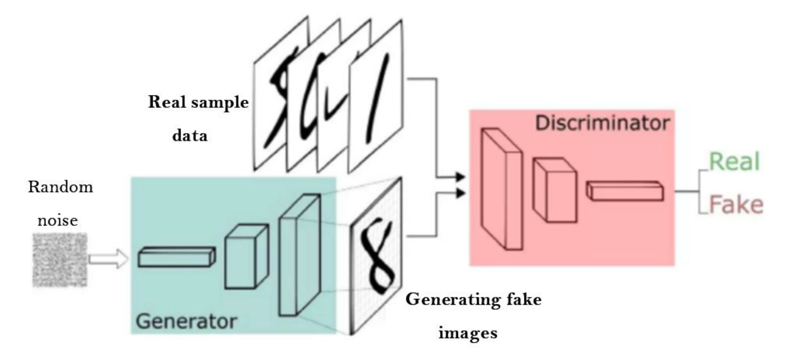
Figure 2.
The diagram of rail fastener shadow image resizing.
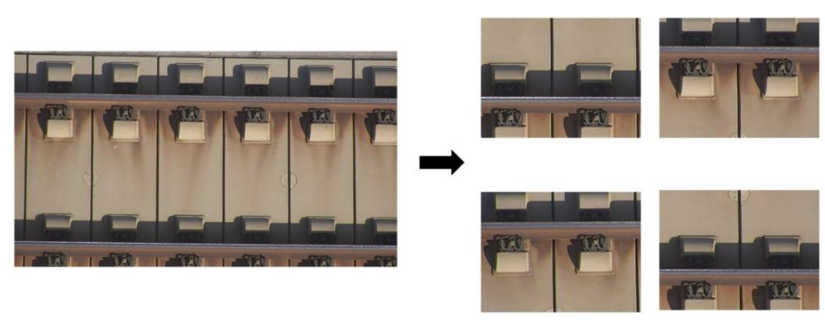
Figure 3.
The diagram of making shadow masks: (a) The original image; (b) The binarized image in Photoshop; (c) The image after fine processing in Photoshop; (d) The shadow mask image.
Figure 3.
The diagram of making shadow masks: (a) The original image; (b) The binarized image in Photoshop; (c) The image after fine processing in Photoshop; (d) The shadow mask image.
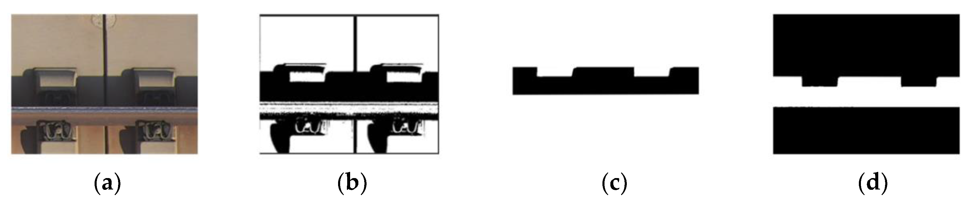
Figure 4.
The construction of pseudo mask generator training data.
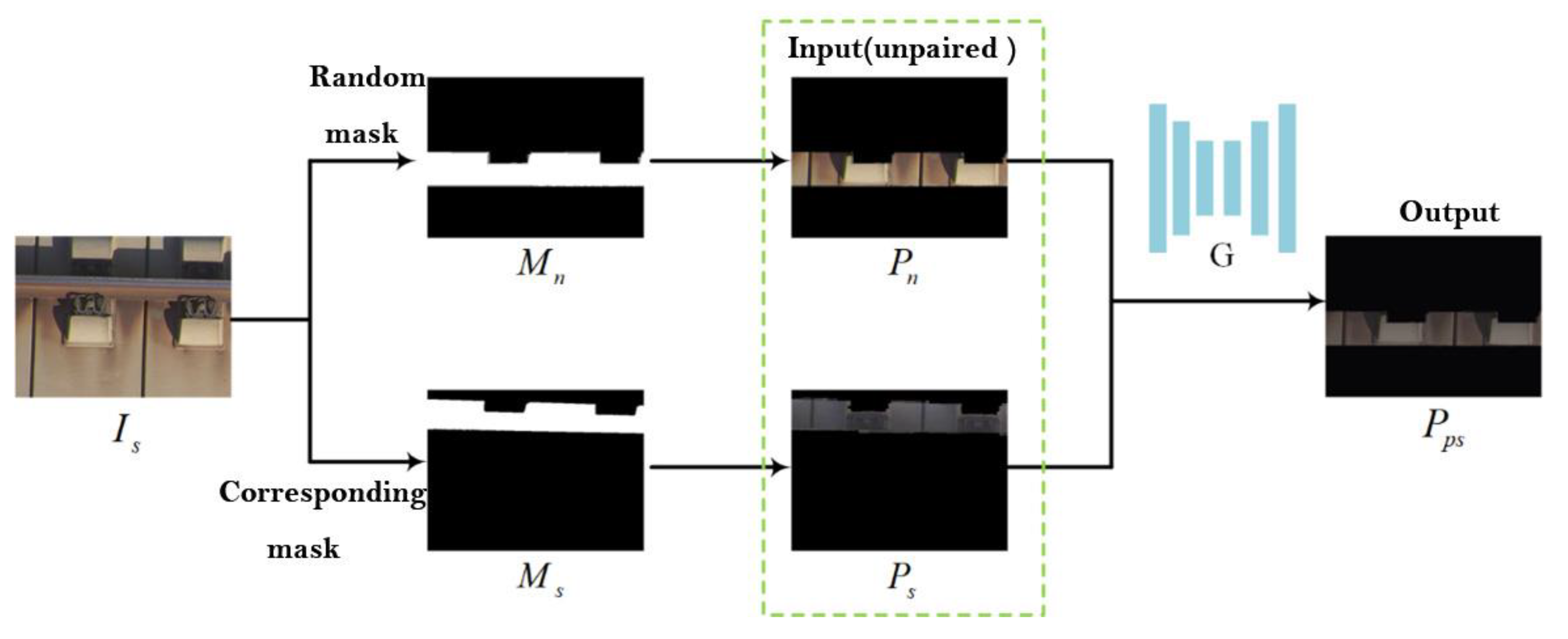
Figure 5.
The construction of shadow removal training data.
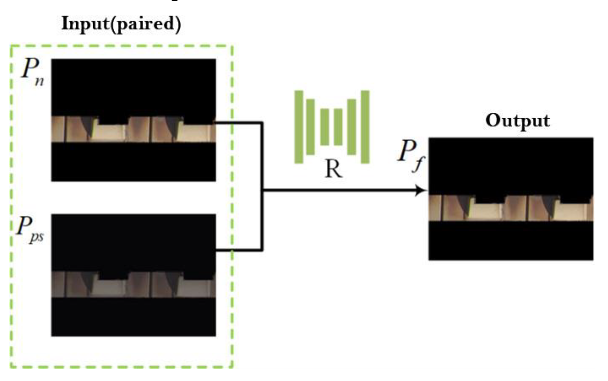
Figure 6.
The framework of Pse-ShadowNet.
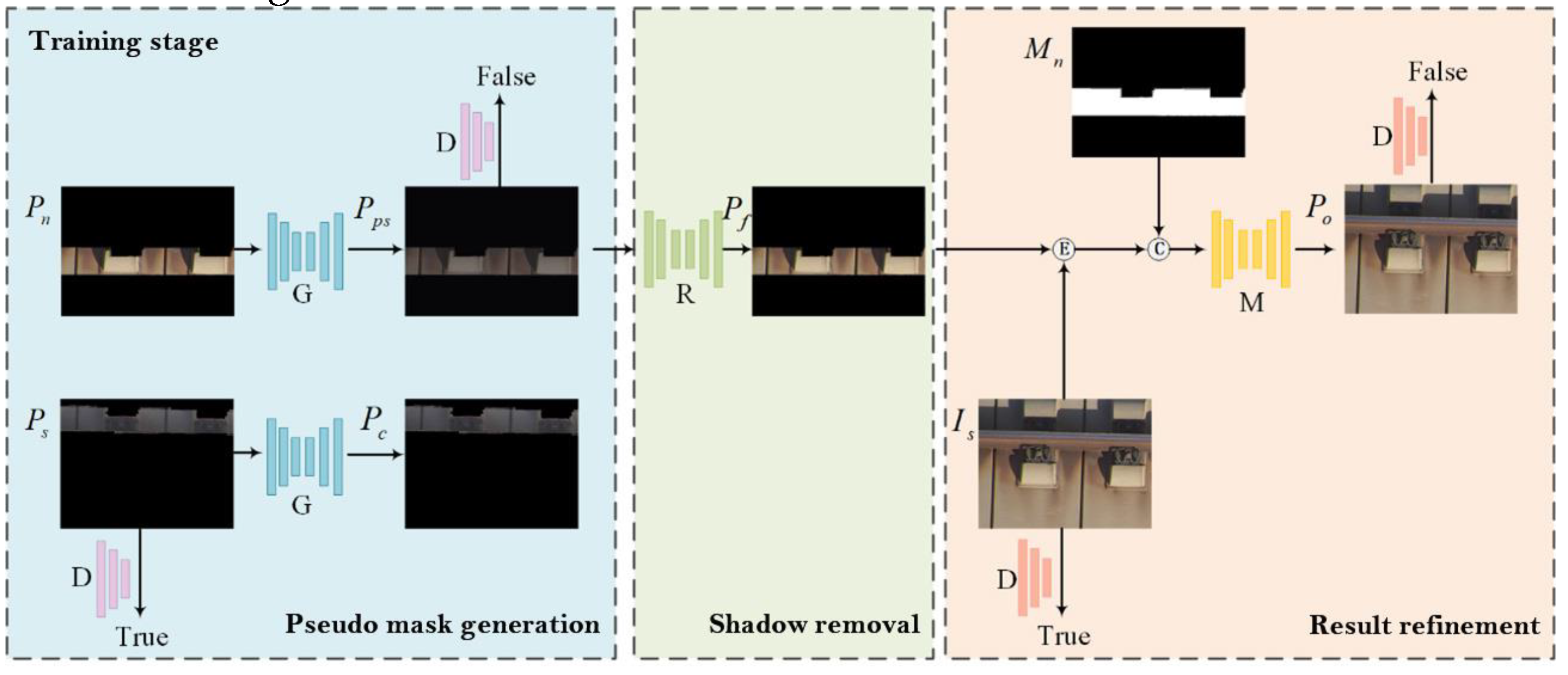
Figure 7.
The testing stage of Pse-ShadowNet.
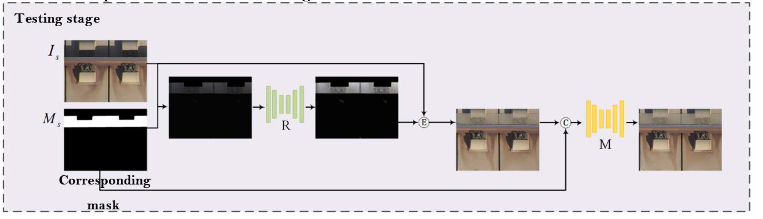
Figure 8.
The structure of the generator network.
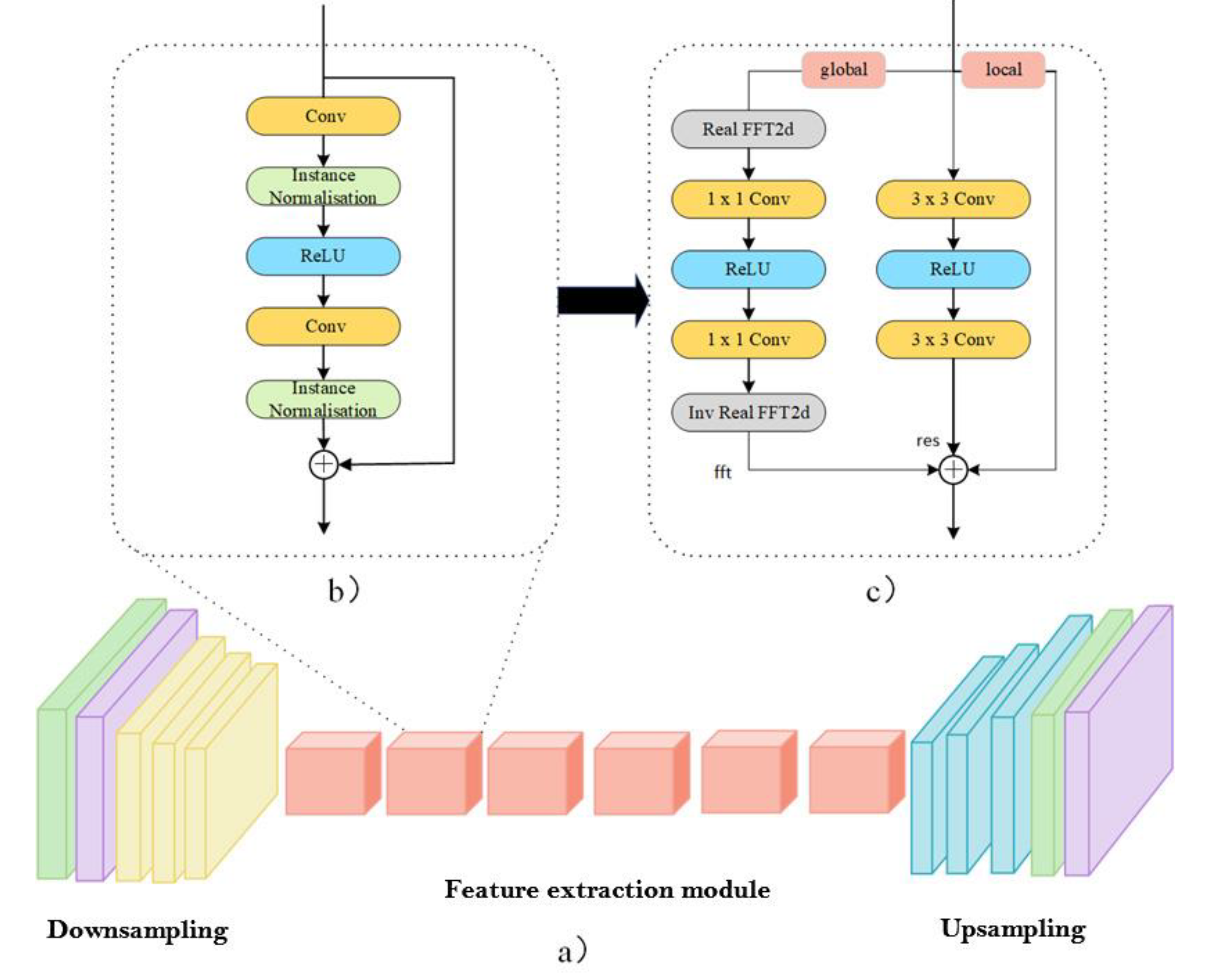
Figure 9.
The structure of discriminator network.
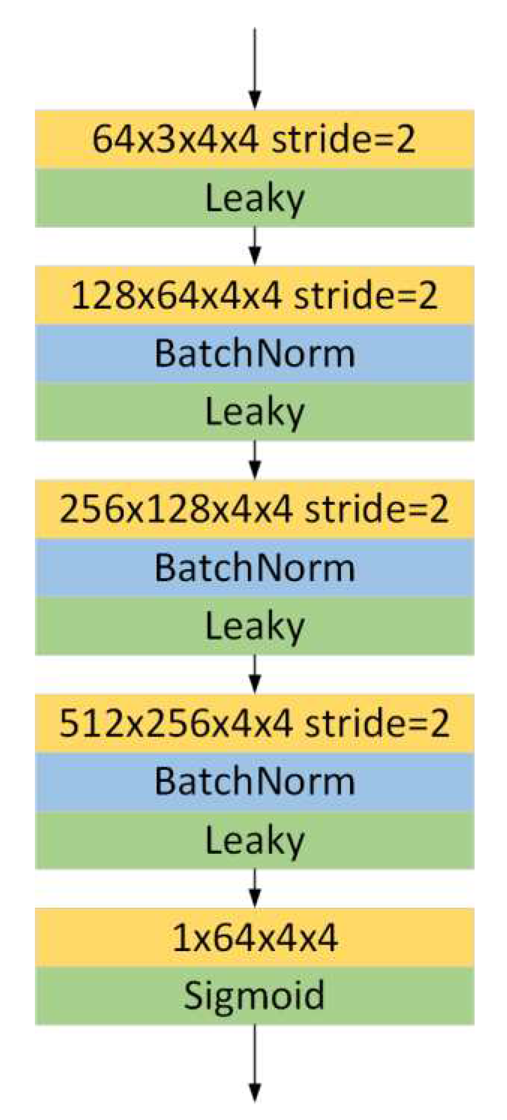
Figure 10.
The principle of the perceptual loss function.
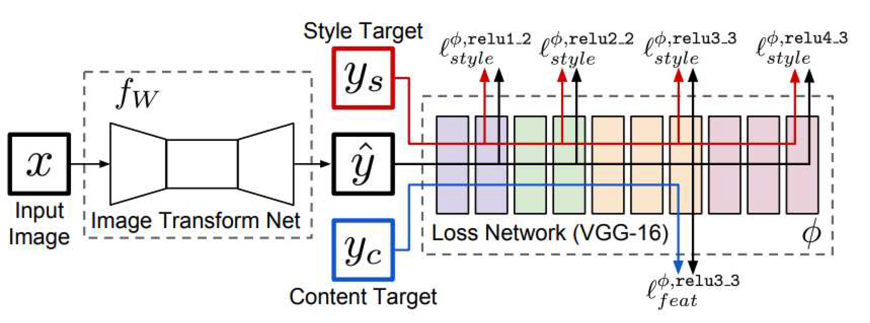
Figure 11.
The training data of the shadow removal network: (a) The original images that require shadow removal; (b) Binary masked images corresponding to the original images.
Figure 11.
The training data of the shadow removal network: (a) The original images that require shadow removal; (b) Binary masked images corresponding to the original images.
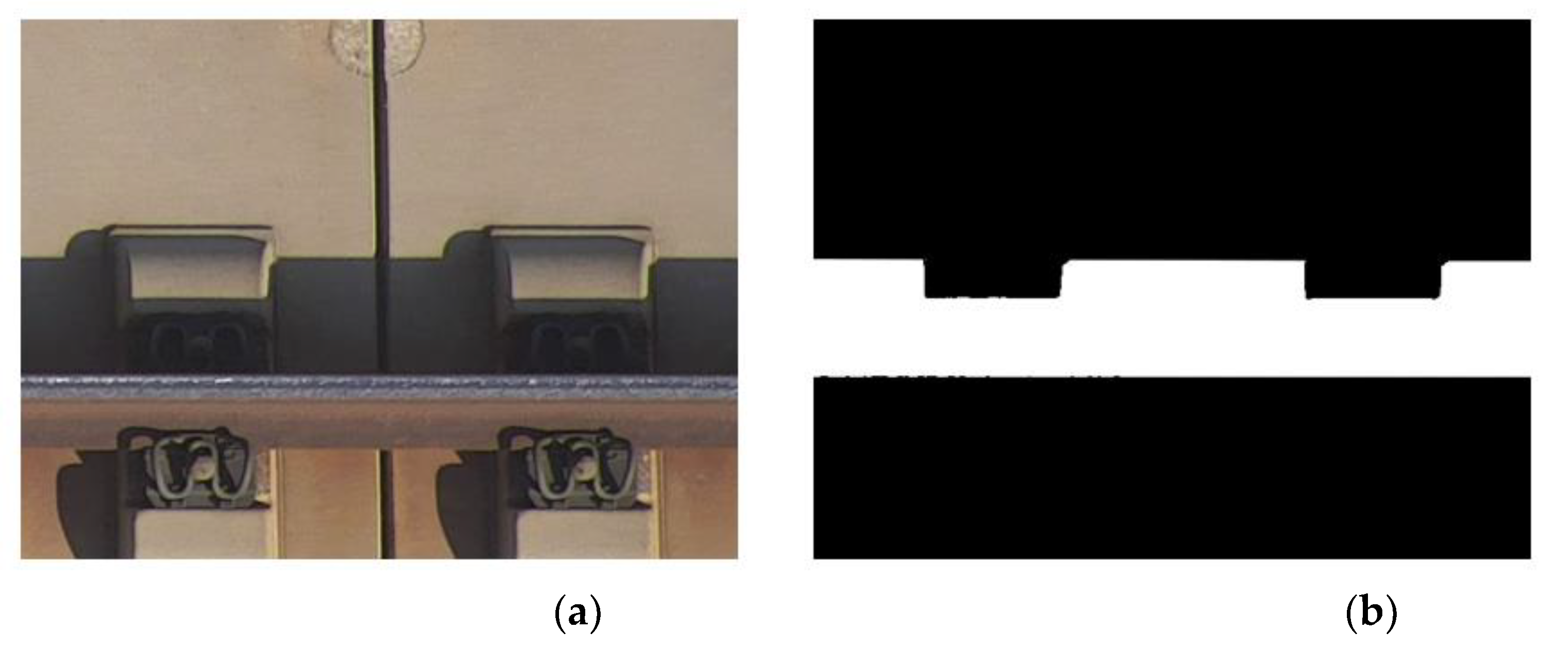
Figure 12.
Comparison of shadow removal results on ISTD dataset:(a) Original shadow image; (b) CycleGAN; (c) Mask-ShadowGAN; (d) LG-ShadowNet; (e) G2R-ShadowNet; (f) Pse-ShadowNetEvaluation on the fastener shadow dataset.
Figure 12.
Comparison of shadow removal results on ISTD dataset:(a) Original shadow image; (b) CycleGAN; (c) Mask-ShadowGAN; (d) LG-ShadowNet; (e) G2R-ShadowNet; (f) Pse-ShadowNetEvaluation on the fastener shadow dataset.
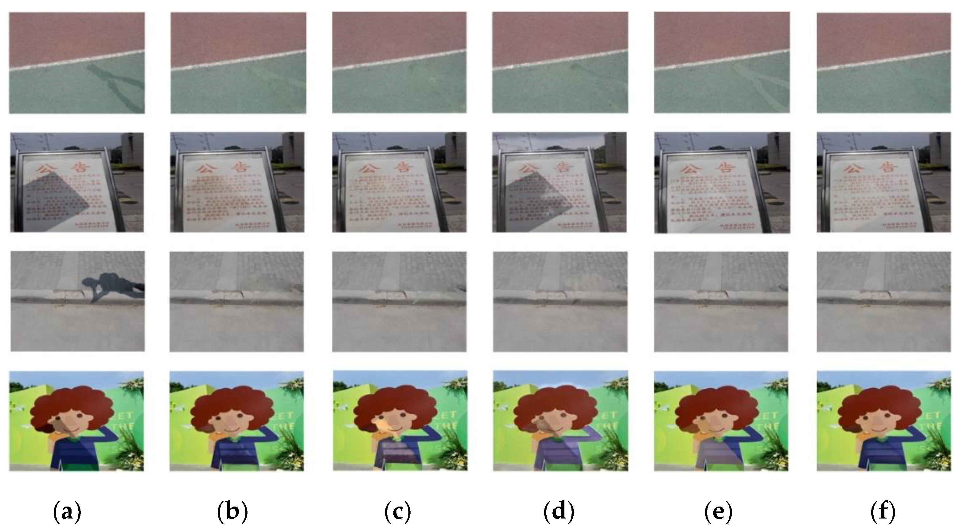
Figure 13.
Comparison of shadow removal results on fastener shadow dataset:(a) Original shadow image; (b) CycleGAN; (c) Mask-ShadowGAN; (d) LG-ShadowNet; (e) G2R-ShadowNet; (f) Pse-ShadowNetQuantitative evaluation.
Figure 13.
Comparison of shadow removal results on fastener shadow dataset:(a) Original shadow image; (b) CycleGAN; (c) Mask-ShadowGAN; (d) LG-ShadowNet; (e) G2R-ShadowNet; (f) Pse-ShadowNetQuantitative evaluation.
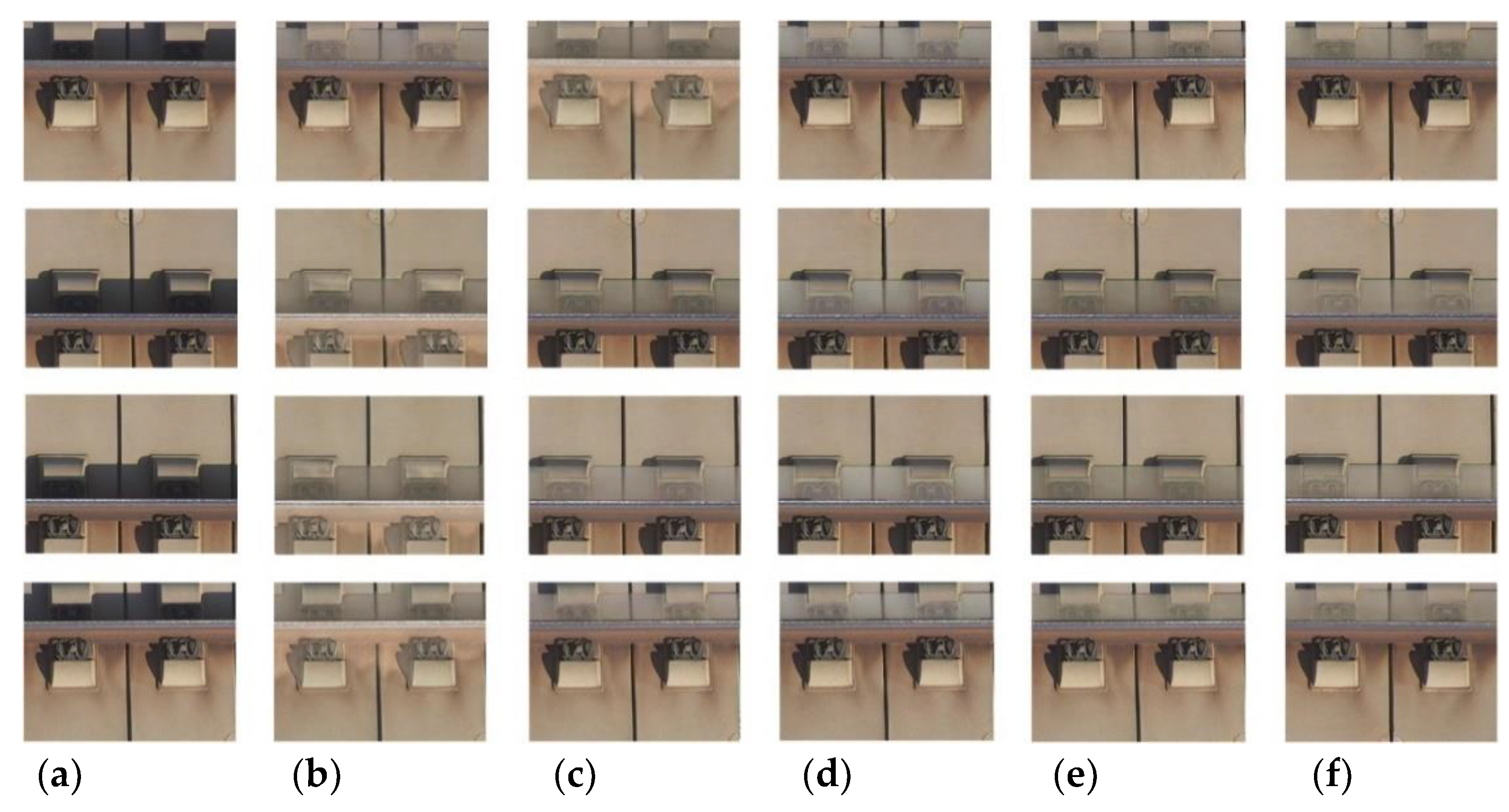
Figure 14.
Structural similarity metrics of different algorithms in the test set.
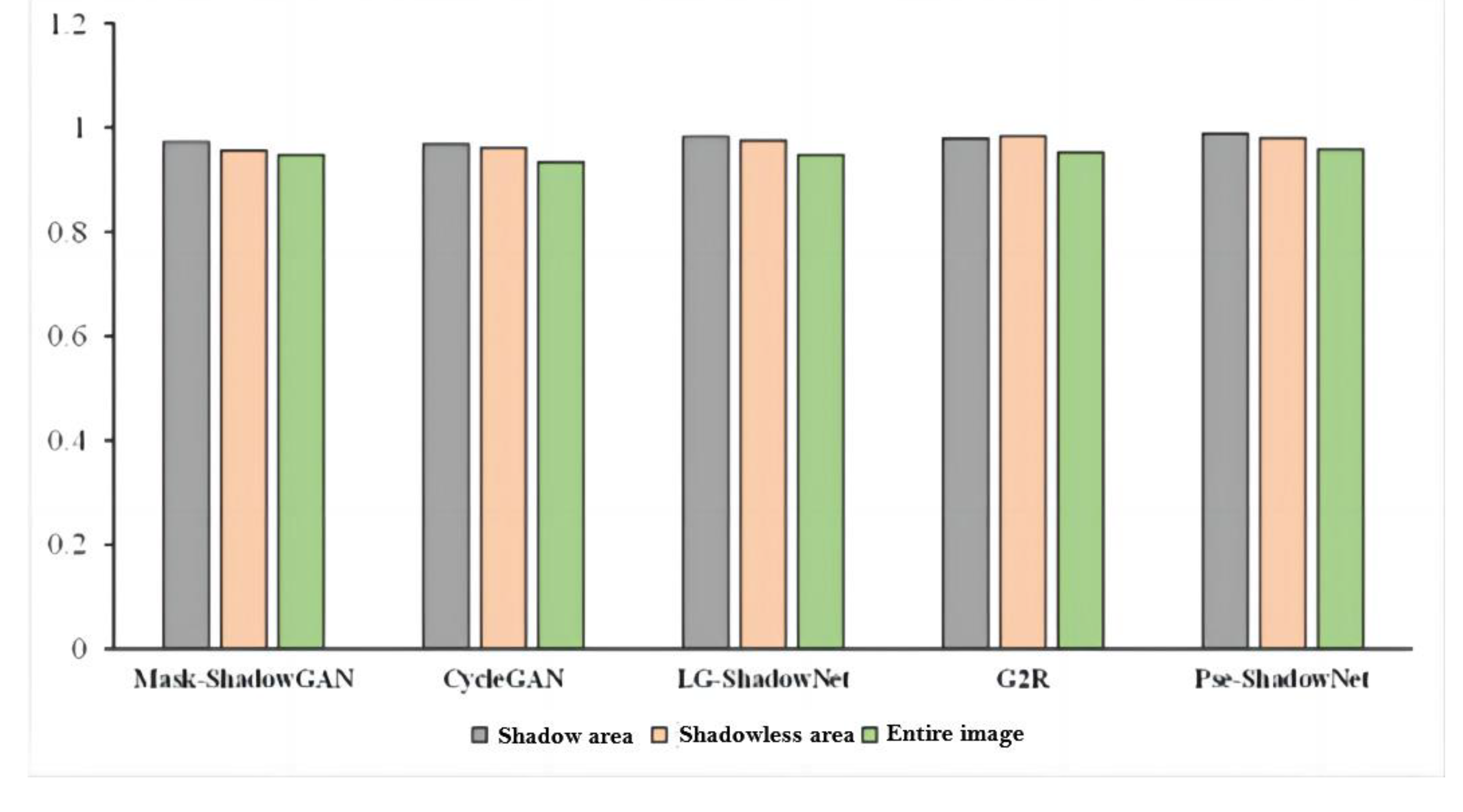
Figure 15.
Peak signal-to-noise ratio of different algorithms in the test set.
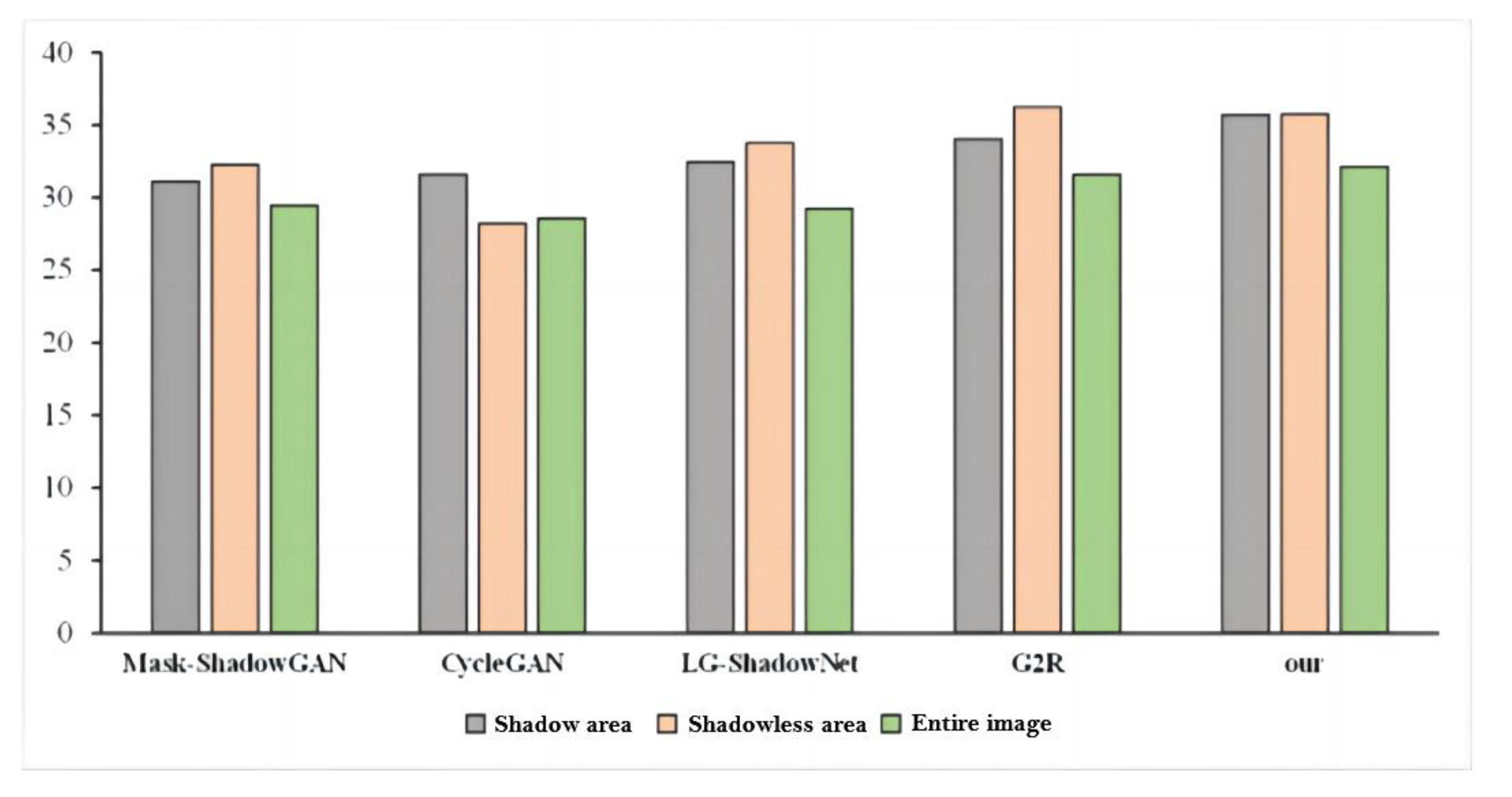
Figure 16.
Comparison of the generated image after introducing the perceptual loss function: (a) The image generated without the perceptual loss function; (b) The image generated with the perceptual loss function.
Figure 16.
Comparison of the generated image after introducing the perceptual loss function: (a) The image generated without the perceptual loss function; (b) The image generated with the perceptual loss function.
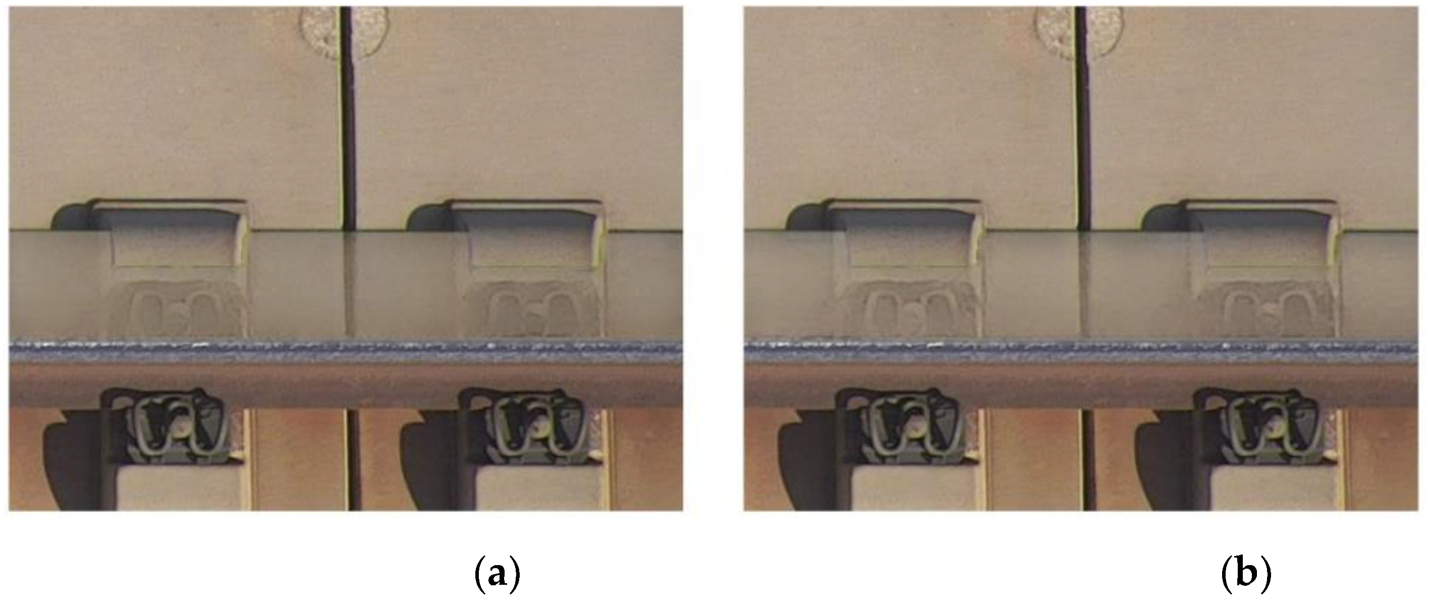
Table 1.
Experiment environment.
| Experimental needs | name | Configure parameters |
|---|---|---|
| Hardware configuration | operating system | Ubuntu 18.04.5 |
| Development language |
Python3.9 | |
| GPU | NVIDIA GeForce GTX 3090ti | |
| Software environment | Tensorflow-gpu | 12.0 |
| Pytorch | 1.10.1 | |
| CUDA | 11.1 | |
| cuDNN | 8.0.4 |
Disclaimer/Publisher’s Note: The statements, opinions and data contained in all publications are solely those of the individual author(s) and contributor(s) and not of MDPI and/or the editor(s). MDPI and/or the editor(s) disclaim responsibility for any injury to people or property resulting from any ideas, methods, instructions or products referred to in the content. |
© 2023 by the authors. Licensee MDPI, Basel, Switzerland. This article is an open access article distributed under the terms and conditions of the Creative Commons Attribution (CC BY) license (http://creativecommons.org/licenses/by/4.0/).
Copyright: This open access article is published under a Creative Commons CC BY 4.0 license, which permit the free download, distribution, and reuse, provided that the author and preprint are cited in any reuse.


