
Submitted:
23 October 2023
Posted:
24 October 2023
You are already at the latest version
Abstract
This paper presents a new discrete counterpart of the mixture exponential distribution by utilizing the survival discretization method. The moment-generating function and associated moment measures are discussed. The distribution’s hazard rate function can assume increasing or decreasing forms, making it adaptable for diverse fields requiring count data modelling. The paper explores four distinct parameter estimation methods and assesses their performance through Monte Carlo simulations. The applicability of this distribution extends to time series analysis, particularly within the framework of the
first-order integer-valued autoregressive process. Additionally, the paper explores quality control applications, addressing serial dependence challenges in count data encountered in production and market management. The performance of two distinct control charts, the cumulative sum chart and the exponentially weighted moving average chart, is evaluated for their effectiveness in detecting shifts in the process means under various models. A bivariate Markov chain approach is used to estimate the average run lengths of these charts, offering valuable insights for implementation. Design recommendations for achieving robustness in-control chart applications are provided. The effectiveness of the proposed models and charts is illustrated using a real data, demonstrating their practical superiority.
Keywords:
Mixture exponential
; INAR(1) process
; CUSUM chart
; EWMA chart
MSC: 60E05; 62M10; 62L10
1. Introduction
In practice, there appears to be a limitless number of count datasets in applied disciplines, indicating the utmost significance of count data modelling. Within this context, discrete probability distributions have assumed a central role in modern data modelling, spanning a diverse spectrum of applied fields. In these practical contexts, count data serve as the fundamental quantification of events occurring within specific intervals. The increasing recognition of the need for more adaptable discrete models is evident, particularly when compared to classical continuous or discrete distributions on the real number line. Although count data modelling has traditionally relied on Poisson and negative binomial distributions, the widespread occurrence of over-dispersion and notable skewness or kurtosis in real-world datasets has emphasized the necessity to create new models. Researchers have responded by introducing innovative discrete distributions through the application of various methodologies and have explored their application in various fields.
Time series models serve as indispensable tools for capturing distinct data features, especially when dealing with count data over time. The first-order integer-valued autoregressive (INAR(1)) process is a significant statistical model for studying auto-correlated count data, excelling in accurately representing counts when compared to Poisson and negative binomial models. Consequently, Al-Osh and Alzaid (1987) introduced the INAR(1) process with binomial thinning having Poisson marginal. Subsequently, other variations, such as the INAR(1) process with Poisson-transmuted exponential innovations proposed by Emrah Altun (2022), and the INAR(1) process with Poisson-extended exponential innovations presented by Maya et al. (2022), have emerged. Researchers are exploring these INAR(1) models to enhance their ability to optimally fit real datasets. This diverse collection of INAR(1) models has garnered substantial interest among researchers, undergoing in-depth exploration and contributing to the evolving landscape of time series modelling.
Statistical quality control primarily focuses on count data and the introduction of control charts has revolutionized this field, making them the primary method for process monitoring. Control charts are designed to maintain process stability and swiftly detect parameter shifts, classifying a process as "in-control" if it adheres to a specified model. Consequently, efficient monitoring is essential to promptly identify shifts in the mean. The cumulative sum (CUSUM) and exponentially weighted moving average (EWMA) control charts, known for their memory capabilities, promptly detect these changes. Conventional control charts, frequently utilized, tend to assume the independence of observations, a premise that may not always be reflected in practical scenarios. This necessitates the utilization of control charts in integer-valued time series models. As a result, Wei and Testik (2009) proposed a CUSUM chart for monitoring the mean of the INAR(1) process with Poisson marginals. Some of the notable works include Li et al. (2022); Kim and Lee (2017); Rakitzis et al. (2017) and Li et al. (2016a). Subsequent to the CUSUM chart, Wei (2011) also discussed the corresponding EWMA chart. Some other works include Wei (2009); Li et al. (2016b) and Li et al. (2019).
Motivated by the aforementioned works, our study introduces a novel discrete mixture exponential (DME) distribution. We utilize survival discretization techniques outlined in Chakraborty (2015) to the mixture exponential (ME) distribution proposed by Mirhossaini and Dolati (2008). In addition to exploring the statistical characteristics of this distribution, our paper presents four distinct parameter estimation approaches. Furthermore, we delve into the application of the DME distribution to an associated INAR(1) process, incorporating DME as innovations.
In the context of process monitoring, we develop control charts tailored for tracking the mean of the proposed process. We investigate the statistical design and performance of CUSUM and EWMA control charts in detecting increasing shifts in process mean levels. Our analysis encompasses the evaluation of control chart properties, particularly their Average Run Length (ARL), which indicates their sensitivity in detecting mean changes within the process. A comparative assessment of both monitoring approaches is also undertaken, providing insights into their effectiveness. Lastly, we assess the practicality of our proposed model by applying it to a real-world data.
The paper is structured as follows: In Section 2, we provide an overview of the construction and characteristics of the DME distribution. Section 3 then introduces the associated statistical properties, including the moment-generating function, moments, skewness, kurtosis, and hazard rate function. Section 4 delves into the discussion of four distinct parameter estimation methods, with an assessment of their performance using Monte Carlo simulations. In Section 5, we evaluate the performance of the proposed distribution using a real dataset. We introduce the INAR(1) process with DME innovations and discuss its properties, including estimation and simulation in Section 6. Section 7 focuses on the statistical process control procedure for INAR(1)DME processes, utilizing the CUSUM and EWMA approaches to detect mean increases, accompanied by numerical simulation and real data analysis. The study is concluded in Section 8.
2. The discrete mixture exponential distribution
The survival discretization method by Chakraborty (2015) is implemented on the continuous mixture exponential distribution, incorporating the reparameterization . As a result, the discrete counterpart is called discrete mixture exponential (DME) distribution. To begin, let us define the continuous ME distribution. The probability density function (pdf) and cumulative distribution function (cdf) of the ME distribution are given by
and
where .
The DME distribution is presented in the following proposition:
Proposition 2.1.
Let DME(, then the probability mass function (pmf) is given by
where and .
The corresponding cdf is given by,
The pmf of the DME distribution always decreases for since
Figure 1 displays the pmf plots of the DME distribution. It can be seen that the DME distribution is rightly skewed and unimodal.
The hazard rate function of the DME distribution is defined as
Figure 2 showcases the DME distribution’s hazard rate function, illustrating its ability to exhibit increasing, decreasing and constant behaviours.
3. Statistical Properties
This section discusses the DME distribution’s moment generating functions, skewness, and kurtosis.
3.1. Moments, Skewness and Kurtosis
Using (2.3), the moment generating function of the DME distribution is given by
The moment about the origin of X is given by,
Using (3.2), the first four raw moments of the DME distribution are given by
Then, the central moments are obtained as,
The moment measures of skewness and kurtosis are given by ,
The dispersion index (DI) of the DME distribution is given by,
The 3D plots in Figure 3 illustrate the graphical representation of skewness and kurtosis, indicating the right-skewed leptokurtic behavior of the DME distribution. From the 3D plot of DI given in Figure 4, we can see that it is always greater than 1. Table 1 illustrates the variation in mean, variance, DI, skewness and kurtosis with respect to the values of and .
4. Estimation
This section describes various methods to estimate parameters for the DME distribution. The methods under consideration include maximum likelihood, ordinary least squares, Anderson-Darling and Cramér–von Mises.
4.1. Maximum likelihood estimation
Let be a sample of size n from DME distribution. Then the likelihood function (L) is given by,
Since and failed to give explicit solutions, the maximum likelihood estimates (MLEs) are obtained by direct maximization of (4.1) using numerical methods.
4.2. Least square estimation
Let be the order statistic of the sample . The least square estimates (LSEs) of the parameters are obtained by minimising the following equation:
4.3. Anderson–Darling Estimation
The Anderson–Darling estimates (ADEs) are obtained using minimising the following equation:
4.4. Cramér–von Mises Estimation
The Cramér–von Mises estimates (CMEs) are obtained by minimising the following equation:
4.5. Simulation
The model performance is analysed by means of a simulation study. The simulation is carried out by taking replications for sample of sizes n = 100, 200, 300, 400 and 500 with different parameter values. The following quantities are computed.
-
Average bias (Bias),Bias()= where is the estimate of the parameter a, for .
-
Root mean square error (RMSE),RMSE
Table 2 lists the Bias and RMSE for the MLEs, LSEs, ADEs and CMEs of the parameters and . We can see that, as n increases, Bias and RMSE decrease. We can conclude that the ML estimation performs very well and is appropriate for small and large sample sizes.
5. Data analysis
We consider the corn-borer data, consisting of the number of European corn-borer larvae pyrausta in the field (Bodhisuwan and Sangpoom (2016)). This data set is taken to compare the performance of the DME distribution with other competitive distributions such as the Poisson distribution, the discrete Burr (DB) distribution (Krishna and Pundir (2009)), the discrete Gumbel (DG) distribution (Chakraborty and Chakravarty (2014)), the discrete log-logistic (DLL) distribution (Para and Jan (2016)), the discrete Bilal (DBL) distribution (Altun et al. (2022)), the discrete Pareto (DPR) distribution (Krishna and Pundir (2009)) and the discrete Rayleigh (DR) distribution (Roy (2004)).
The unknown parameters are obtained using the ML method, along with the standard error (SE) and 95% confidence interval (CI) for various considered models. Model performance is assessed using some widely accepted information criteria and goodness-of-fit statistics. Smaller values of the Akaike information criterion (AIC) and Bayesian information criterion (BIC), as well as larger log-likelihood (log L) values, indicate the adequacy of the model. Furthermore, we employ a test to evaluate the goodness-of-fit for each fitted distribution, with a small value and a large p-value indicating a good fit.
Table 3 makes it abundantly clear that the DME distribution is the best of the competitive models under consideration because it has the lowest AIC and BIC, the highest log L and p-value, repectively. Table 4 gives the observed and expected frequencies of corn-borer data under various distributions. Figure 5 indicates better modelling of DME distribution over all the models considered.
6. INAR(1) process with discrete mixture exponential innovations
In this section, we develop the INAR(1) process with innovations following the DME distribution. We consider INAR(1) time series models using the binomial thinning operator with independent Bernoulli counting series random variables. Hereafter, the introduced INAR(1) process with the DME distributed innovations shall be denoted as INAR(1)DME process.
6.1. INAR(1)DME process
The INAR(1)DME process is given by
where "∘" is the binomial thinning operator, is a sequence of independent and identically distributed (iid) random variables from DME() distribution and is independent of Bernoulli counting process and for all . The binomial thinning operator is generated by counting series of independent Bernoulli distributed random variables and is defined as
where X is a non-negative integer-valued random variable and is a sequence of independent and identically distributed random variables with Bernoulli distribution and is independent of X.
The one-step transition probability of the INAR(1) process is given by,
The one-step transition probability of the INAR(1)DME process is given by,
Also, the stationary marginal density of is given by,
Then, the DI of is given by,
Table 5 provides the DI of across different parameter configurations, indicating the model’s ability to accommodate over-dispersed data. The one-step-ahead conditional mean and variance of the INAR(1)DME process are given by,
6.2. Estimation
6.2.1. Conditional maximum likelihood
The knowledge of the transition probabilities is sufficient for the creation of the likelihood function in the conditional ML (CML) technique. For a given sample from the INAR(1)DME process, the conditional log-likelihood function is given by,
where is fixed, and is given by (6.4). The CML estimates (CMLEs) of the parameters p, are obtained by maximizing (6.11) using the optim function in R software.
6.2.2. Conditional least square estimation
The conditional least square estimates (CLSEs) of parameters p, are obtained by minimising the following equation,
6.3. Simulation
A simulation study was performed to assess the performance of the CML and CLS estimation methods under the INAR(1)DME process. The simulation is carried out by taking 1,000 replications for samples of sizes n = 50, 100, 150, 200, and 250 with different parameter values, and the following quantities were computed.
-
Average bias (Bias) of the parameters,Bias()= where is the estimate of
-
Root mean square error (MSE) of the parameters,RMSE
From Table 6, we can see that as n increases, Bias and RMSE decrease. We can conclude that the CML estimation method performs very well and is appropriate for small and large sample sizes.
7. Control charts for monitoring mean of the INAR(1)DME process
This section explores an efficient control chart for monitoring the INAR(1)DME process. In INAR(1) processes, upward shifts in the process mean indicate a collective rise in associated factors for entities, such as unemployment rate, defect percentage, and disease spread. Identification and timely reporting of such shifts are typically vital. Therefore, with a focus on practical applications, this paper investigates the mean upward shift within the INAR(1)DME process.
We construct the upper-sided control chart to focus exclusively on detecting upward shifts in as it is directly linked to process deterioration. The main purpose is to detect quickly and accurately a change in the ; it is more natural to monitor the process of directly by taking care of the impact of autocorrelation. A process is considered in-control when it adheres to a specified model. Conversely, a process is deemed out of control when the parameters within the model change rather than the model itself undergoing a change. When the process is in-control, the parameter values of the INAR(1)DME process will be denoted as , and . An increasing shift in may occur if one of the parameters p, and have changed appropriately.
We observe from Table 7 that is affected by variations in the parameter within the INAR(1)DME process, resulting in a higher value of . To effectively monitor INAR(1) processes, we employ CUSUM and EWMA control charts and assess the efficiency of these monitoring techniques.
7.1. The CUSUM chart
Initially proposed by Page (1961), the CUSUM chart operates on the fundamental principle of the sequential probability ratio test. Its primary objective is to gather and accumulate information from sample data, thus magnifying the impact of minor process deviations. Numerous studies have extensively demonstrated the effectiveness of the CUSUM chart in monitoring time series comprising of integer values, including Poisson INAR(1) by Wei and Testik (2009) and Wei and Testik (2011), geometrically inflated Poisson INAR(1) by Li et al. (2022), new geometric INAR(1) by Li et al. (2016a) and zero-inflated Poisson INAR(1) by Rakitzis et al. (2017).
Here, we devise the CUSUM control charts due to their sensitivity in detecting small shifts. Furthermore, CUSUM charts also have known optimality properties when detecting a sustained shift from a known in-control distribution to a specified out-of-control distribution (Wei and Testik (2009)).
From Wei and Testik (2009), let . A CUSUM statistic with reference value k is obtained as,
Here is the starting value. For , the monitoring statistics are plotted on a CUSUM chart with control region [0, h], where h is the upper control limit. The INAR(1)DME process is considered as being in-control unless . The reference value k prevents the chart from drifting towards control limits during in-control processes and offers the ability to fine-tune chart sensitivity to specific shifts in the process mean.
7.2. The EWMA chart
Initially proposed by Roberts (2000), the EWMA chart operates on the fundamental principle of giving the highest weight to the nearest samples in the time series, while previous samples contribute minimally. The EWMA chart is useful for detecting persistent shifts for INAR processes (Wei (2009)).
From Wei (2011), let and . An EWMA statistic of the INAR(1) process is given by,
where if and only if the integer . Let with . The statistics are plotted on an EWMA chart with control region , where u is the upper control limit. The process is considered as being in-control unless an out-of-control signal is triggered.
7.3. Performance of the INAR(1)DME control charts
The average run length (ARL) is a commonly used measure to evaluate the effectiveness of a control chart in statistical process control. It represents the expected number of data points plotted on the control chart before it signals an out-of-control condition. Two specific types of ARL are considered: , also known as in-control ARL, measures the number of data points plotted from the beginning of monitoring until a false alarm is triggered. On the other hand, referred to as out-of-control ARL, quantifies the number of data points plotted from the start of a process shift until the chart detects that shift. To have an effective control chart, a high combined with a small is essential.
7.3.1. ARL of CUSUM chart
For a given , the values of are chosen to ensure that the closely matches a specified value. As of the INAR(1)DME process forms a bivariate Markov chain, the Markov chain approach introduced in Wei and Testik (2009) is used here for computing ARL. To offer a comprehensive overview, the computational approach is briefly outlined as follows.
Let us consider the case where . Whenever , it leads to an out-of-control signal since exceeds h if and only if . Hence, the attainable in-control range of needs to be restricted. From Wei and Testik (2009), under the CUSUM chart, the set of attainable in-control values for the bivariate Markov process is given by,
which is of size
The above arguments can also be extended if and are permitted to assume values from the set , where the common denominator .
The initial probabilities are,
where denotes the Kronecker delta, and are given by (6.4) and (6.5) respectively.
Also, the conditional probability that the run length of equals r is given by
where .
Let the vector denote the factorial moments, given by,
where,
Then,
That is, is the solution of the linear equation . The dimension of Q and is determined by (7.4). Hence, the ARL depending on the initial choice , is defined as,
7.3.2. ARL of EWMA chart
For a given , the values of are chosen to ensure that the closely matches a specified value. Subsequently, the ARL values are calculated using the model parameters and EWMA chart designs. As of the INAR(1)DME process forms a bivariate Markov chain, the Markov chain approach introduced in Wei (2011) is used here for computing ARL. To offer a comprehensive overview, the computational approach is briefly outlined as follows.
Let denote the smallest integer value greater than or equal to x. From Wei (2011), under the EWMA chart, the set of attainable in-control values for the bivariate Markov process is given by,
The transition and initial probabilities of is given by,
where
The initial probabilities are,
where denote the indicator function.
Also, the conditional probability that the run length of equals r is given by
where .
Let the vector denote the factorial moments, given by,
where
Then,
That is, is the solution of the linear equation .
Hence, the depending on the initial choice , is defined as,
7.4. Numerical simulation
Now, we will assess the performance of both CUSUM and EWMA in detecting changes in the process mean by means of a simulation study. The central aim of our investigation pertains to detecting changes in the parameter . Table 8 presents a comprehensive depiction of the variability observed in across the various values of the parameter with respect to = -0.1 and 0.9. The deviations are calculated according to , where is the mean associated with the parameters . We obtain the desired chart designs such that the desired in-control ARL value, is 300. Due to the complexity of (6.5), the marginal probabilities are empirically obtained through a simulated process of desirable size at given . Besides ARL as a performance measure for the control charts, we have also incorporated the usual relative deviation (in %) in the ARL from Wei and Testik (2011), given as to assess and evaluate the efficacy and performance of the chart.
Under the CUSUM chart, for a given , our focus revolves around possible integer h and k pairs such that the desired in-control ARL is close to . For the EWMA chart, the design parameters are obtained as follows
- Choose such that a corresponding one-sided C chart would have an in-control ARL below the desired value .
- Decrease to adjust the in-control ARL close to the desired value . Subsequently, in the combined EWMA chart is calculated accordingly as .
- Use for a fine-tuning of the in-control ARL.
Subsequently, the ARL values are calculated using the model parameters and chart designs.
In Table 9 and Table 10, we examine the performance of ARL under CUSUM chart with with various values of respectively. The results show the high efficacy of the CUSUM chart in detecting upward shifts in . Specifically, we observed a remarkable decrease in the ARL as increases. Furthermore, it is important to note that the decline in ARL is significantly greater than the corresponding rise in the magnitude of the shift in .
Hence, it can be concluded that the CUSUM control chart demonstrates effective performance when applied to the INAR(1)DME process. The chart’s ability to efficiently detect upward shifts in makes it a suitable and beneficial tool for monitoring and controlling the INAR(1)DME process.
against various values of , respectively. The results show the high efficacy of the EWMA chart in detecting upward shifts in . Specifically, we observed a remarkable decrease in the ARL as increases. Furthermore, it is important to note that the decline in ARL is significantly greater than the corresponding rise in the magnitude of the shift in . Hence, it can be concluded that the EWMA control chart demonstrates effective performance when applied to the INAR(1)DME process. The chart’s ability to efficiently detect upward shifts in makes it a suitable and beneficial tool for monitoring and controlling the INAR(1)DME process.
Table 13 provides a comparative analysis of CUSUM and EWMA charts within the context of the INAR(1)DME process, considering specific values of . Bolded entries indicate instances where the dev(%) is maximized between the two charts sharing the same model parameters. It becomes evident that both charts exhibit a more significant reduction in ARL as increases. When monitoring data from the INAR(1)DME process and accounting for various shift sizes, the CUSUM chart is the preferred choice for maintaining process control.
7.5. Real data analysis
We demonstrate the applicability of the CUSUM control chart by utilizing the disorderly conduct data set obtained from the 44th police car beat in Pittsburgh, which comprises monthly observations from 1990 to 2001. It is used to monitor the mean under the INAR(1)KF process by Kim and Lee (2017). Initially, we use the data from 1990 to 1996 to fit the INAR(1)DME process. Subsequently, we apply the CUSUM control chart to the data from 1997 to detect the presence of any significant mean increase.
Figure 6 displays the time series plot of the disorderly conduct data set (the dashed line denotes December 1996). Based on the plot, detecting the mean shift after the dashed line is challenging. For the data from 1990 to 1996 (Phase I data), the sample mean, and variance are obtained as 3.9643 and 5.3602, respectively. Figure 7 displays the auto correlation function (ACF) and partial ACF (PACF) plots for the phase I data. Here, only the first lag is significant in the PACF plot, and the ACF plot displays an exponential decay, facilitating to model the data as an INAR(1) process. Hence, we proceed by modelling the data using the INAR(1)DME model and other competing models on the phase I data. The following are considered:
- INAR(1) process with Poisson marginals, Al-Osh and Alzaid (1987) (INARP(1))
- quasi-binomial INAR(1) process with generalized Poisson marginals, Alzaid and Al-Osh (1993) ( QINARGP(1))
- iterated INAR(1) process with negative binomial marginals, Al-Osh and Aly (1992) (IINARNB(1))
- INAR(1) process with geometric marginals, Alzaid and Al-Osh (1988) (INARG(1))
- INAR(1) process with zero-inflated Poisson innovations, Jazi et al. (2012) (INAR(1)ZP)
- INAR(1) process with geometric innovations, Aghababaei Jazi et al. (2012) (INAR(1)G)
- INAR(1) process with Katz family innovations, Kim and Lee (2017) (INAR(1)KF)
Table 14 lists the CMLEs, log L, AIC, BIC and for different processes. The maximum log L and minimum AIC and BIC values for the INAR(1)DME process show that it is a better fit than the contending models.
To check whether the fitted INAR(1)DME process is statistically accurate, residual analysis is done with the Pearson residuals. The ACF of the Pearson residuals is displayed in Figure 8, showing that there is no autocorrelation for the Pearson residuals. To ensure this, the Ljung–Box test for the presence of autocorrelation is done with degrees of freedom 10 and has the p-value = 0.957 > 0.05. It indicates that they are uncorrelated. Also, the mean and variance of Pearson residuals are 0.00228 and 0.83, close to the preferred values of 0 and 1, respectively, validating a good fit. Hence, the INAR(1)DME process fits the phase I data well.
The cpgrams of Pearson residuals of phase I is displayed in Figure 9. We can see that the residuals exhibit random behaviour without trend distribution for the phase I data.
The INAR(1)DME model for the phase I data is given by,
where DME(-0.9999, 0.5957).
The predicted values can be obtained by,
Figure 10 displays the time series plot of the original versus predicted values for the phase I data.
Now, we consider the CUSUM chart with reference value k=4 (Kim and Lee (2017)) based on the INAR(1)DME process with parameters () and a suitable limit value h is chosen.
Table 15 provides the ARL values with respect to INAR(1)DME, INAR(1)KF and INARP(1) processes for and , respectively. Here the INAR(1)DME process outperforms the others since it has less ARL values. Taking , the upper control limit CUSUM chart under the INAR(1)DME process is obtained as .
The CUSUM chart for disorderly conduct data under INAR(1)DME process is given in Figure 11, where the red horizontal dashed and vertical dashed lines respectively stand for and December 1996.
From the plot, we can see that occurred in May 2000. The sample mean of the data from January 1997 to May 2000 is 4.7073, which is greater than that of the past observations. Identifying this phenomenon is challenging unless the CUSUM control scheme has been implemented.
8. Conclusion
Our paper presents a novel discrete analogue of the mixture exponential distribution, generated through survival discretization, with a strong emphasis on its statistical properties and the discussion of four distinct estimation methods. These methods play a pivotal role in this research, offering robust tools for parameter estimation. We further explore the application of this distribution in an associated INAR(1) process with DME innovations, conducting a comprehensive investigation into its statistical characteristics and performance through extensive simulation studies. Our work also extends to the domain of process monitoring, where we develop custom control charts tailored to track the process mean. In this context, we meticulously analyze the effectiveness of CUSUM and EWMA control charts in detecting shifts and provide valuable insights through comparative assessments. Additionally, the practical applicability of our proposed model is confirmed through its use with real-world data under the CUSUM chart, showcasing its relevance in both statistical theory and real-world process monitoring and control applications.
References
- M. Aghababaei Jazi, G. Jones, and C.-D. Lai. 2012 Integer valued AR (1) with geometric innovations. Journal of the Iranian Statistical Society 11: 173–190.
- M. A. Al-Osh, and E.-E. A. Aly. 1992. First order autoregressive time series with negative binomial and geometric marginals. Communications in Statistics-Theory and Methods 21: 2483–2492.
- M. A. Al-Osh, and A. A. Alzaid. 1987. First-order integer-valued autoregressive (INAR(1)) process. Journal of Time Series Analysis 8: 261–275. [CrossRef]
- E. Altun, M. El-Morshedy, and M. Eliwa. 2022. A study on discrete Bilal distribution with properties and applications on integer valued autoregressive process. REVSTAT-Statistical Journal 20: 501–528. [Google Scholar]
- A. Alzaid, and M. Al-Osh. 1988. First-order integer-valued autoregressive (INAR(1)) process: distributional and regression properties. Statistica Neerlandica 42: 53–61. [CrossRef]
- A. A. Alzaid, and M. A. Al-Osh. 1993. Some autoregressive moving average processes with generalized Poisson marginal distributions. Annals of the Institute of Statistical Mathematics 45: 223–232. [CrossRef]
- W. Bodhisuwan and S. Sangpoom. The discrete weighted Lindley distribution. In 2016 12th International Conference on Mathematics, Statistics, and Their Applications (ICMSA), pages 99–103. IEEE, 2016.
- S. Chakraborty. 2015. Generating discrete analogues of continuous probability distributions - a survey of methods and constructions. Journal of Statistical Distributions and Applications 2: 1–30.
- S. Chakraborty, and D. Chakravarty. 2014. A discrete Gumbel distribution. arXiv preprint arXiv:1410.7568.
- N. M. K. Emrah Altun. 2022. Modelling with the novel INAR(1)-PTE process. Methodol Comput Appl Probab 24: 1735–1751.
- M. A. Jazi, G. Jones, and C.-D. Lai. 2012. First-order integer valued AR processes with zero inflated Poisson innovations. Journal of Time Series Analysis 33: 954–963. [Google Scholar] [CrossRef]
- H. Kim, and S. Lee. 2017. On first-order integer-valued autoregressive process with Katz family innovations. Journal of Statistical Computation and Simulation 87: 546–562. [CrossRef]
- H. Krishna, and P. S. Pundir. 2009. Discrete Burr and discrete Pareto distributions. Statistical methodology 6: 177–188. [CrossRef]
- C. Li, D. Wang, and F. Zhu. 2016a. Effective control charts for monitoring the NGINAR(1) process. Quality and Reliability Engineering International 32: 877–888. [Google Scholar] [CrossRef]
- C. Li, D. Wang, and F. Zhu. 2016b. Effective control charts for monitoring the NGINAR (1) process. Quality and Reliability Engineering International 32: 877–888. [Google Scholar] [CrossRef]
- C. Li, D. Wang, and F. Zhu. 2019. Detecting mean increases in zero truncated inar (1) processes. International Journal of Production Research 57: 5589–5603. [Google Scholar] [CrossRef]
- C. Li, H. Zhang, and D. Wang. 2022. Modelling and monitoring of INAR(1) process with geometrically inflated Poisson innovations. Journal of Applied Statistics 49: 1821–1847. [Google Scholar] [CrossRef] [PubMed]
- R. Maya, C. Chesneau, A. Krishna, and M. R. Irshad. 2022. Poisson extended exponential distribution with associated INAR(1) process and applications. Stats 5: 755–772. [Google Scholar] [CrossRef]
- E. McKenzie. 1986. Autoregressive moving-average processes with negative-binomial and geometric marginal distributions. Advances in Applied Probability 18: 679–705. [CrossRef]
- S. M. Mirhossaini, and A. Dolati. 2008. On a new generalization of the exponential distribution. Journal of Mathematical Extension.
- E. Page. 1961. Cumulative sum charts. Technometrics 3: 1–9.
- B. A. Para and T. R. Jan. 2016. Discrete version of log-logistic distribution and its applications in genetics. Int. J. Mod. Math. Sci 14: 407–422.
- A. C. Rakitzis, C. H. Weiß, and P. Castagliola. 2017. Control charts for monitoring correlated Poisson counts with an excessive number of zeros. Quality and Reliability Engineering International 33: 413–430. [Google Scholar] [CrossRef]
- M. M. Ristić, H. S. Bakouch, and A. S. Nastić. 2009. A new geometric first-order integer-valued autoregressive (NGINAR(1)) process. Journal of Statistical Planning and Inference 139: 2218–2226. [Google Scholar] [CrossRef]
- M. M. Ristić, A. S. Nastić, and A. V. Miletić Ilić. 2013. A geometric time series model with dependent bernoulli counting series. Journal of Time Series Analysis 34: 466–476. [Google Scholar] [CrossRef]
- S. Roberts. 2000. Control chart tests based on geometric moving averages. Technometrics 42: 97–101. [CrossRef]
- D. Roy. 2004. Discrete Rayleigh distribution. IEEE transactions on reliability 53: 255–260.
- C. H. Weiß. 2008. Thinning operations for modeling time series of counts—a survey. AStA Advances in Statistical Analysis 92: 319–341.
- C. H. Weiß. 2009. EWMA monitoring of correlated processes of Poisson counts. Quality Technology & Quantitative Management 6: 137–153.
- C. H., Weiß. 2011. Detecting mean increases in Poisson INAR (1) processes with EWMA control charts. Journal of Applied Statistics 38: 383–398. [Google Scholar]
- C. H., Weiß. 2018. An introduction to discrete-valued time series. John Wiley & Sons. [Google Scholar]
- C. H. Weiß, and M. C. Testik. 2009. CUSUM monitoring of first-order integer-valued autoregressive processes of Poisson counts. Journal of quality technology 41: 389–400. [CrossRef]
- C. H. Weiß, and M. C. Testik. 2011. The Poisson INAR(1) CUSUM chart under overdispersion and estimation error. IIE Transactions 43: 805–818. [CrossRef]
Figure 1.
Pmfs of the DME distribution for different parameter values.
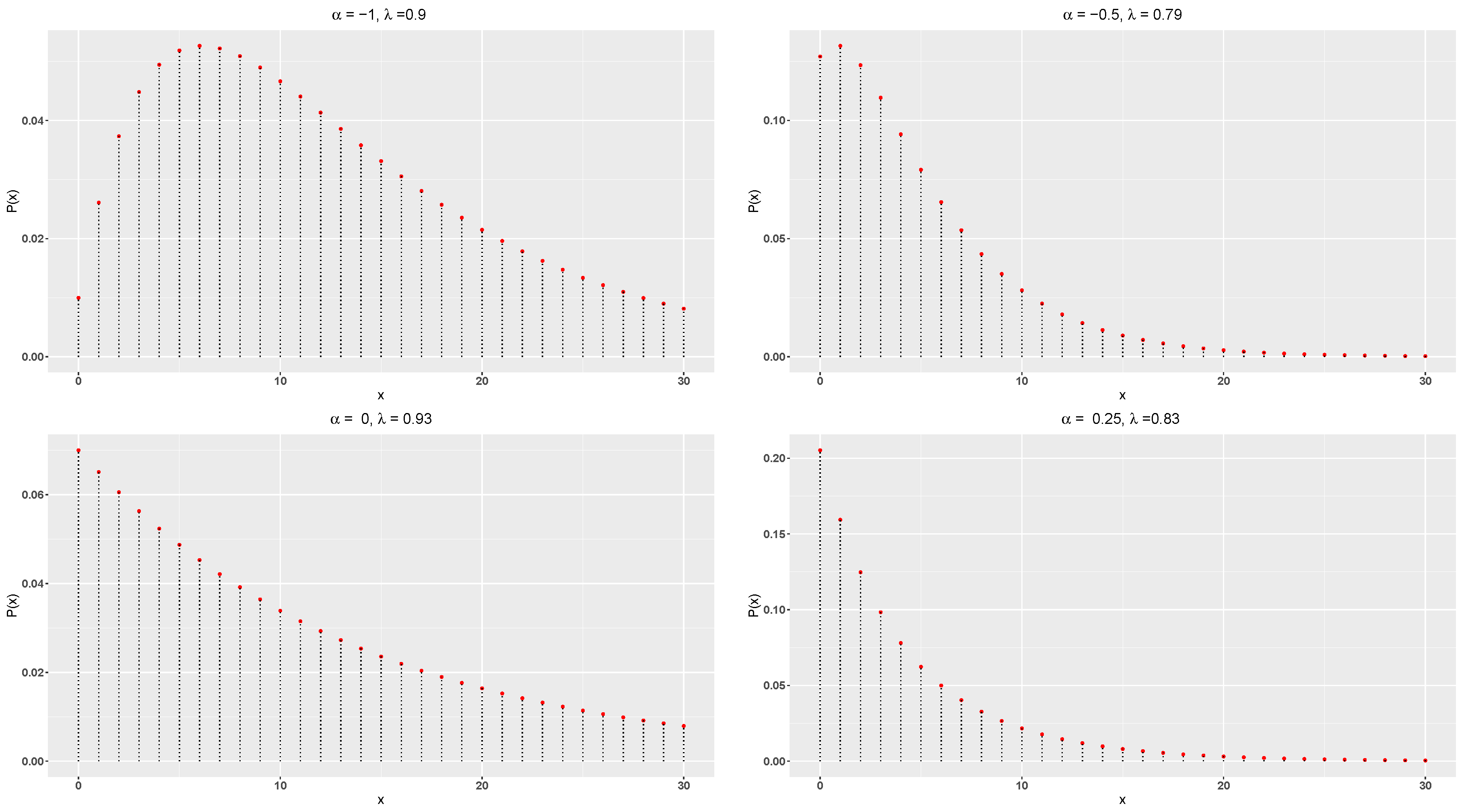
Figure 2.
hazard rate function of the DME distribution for different parameter values.
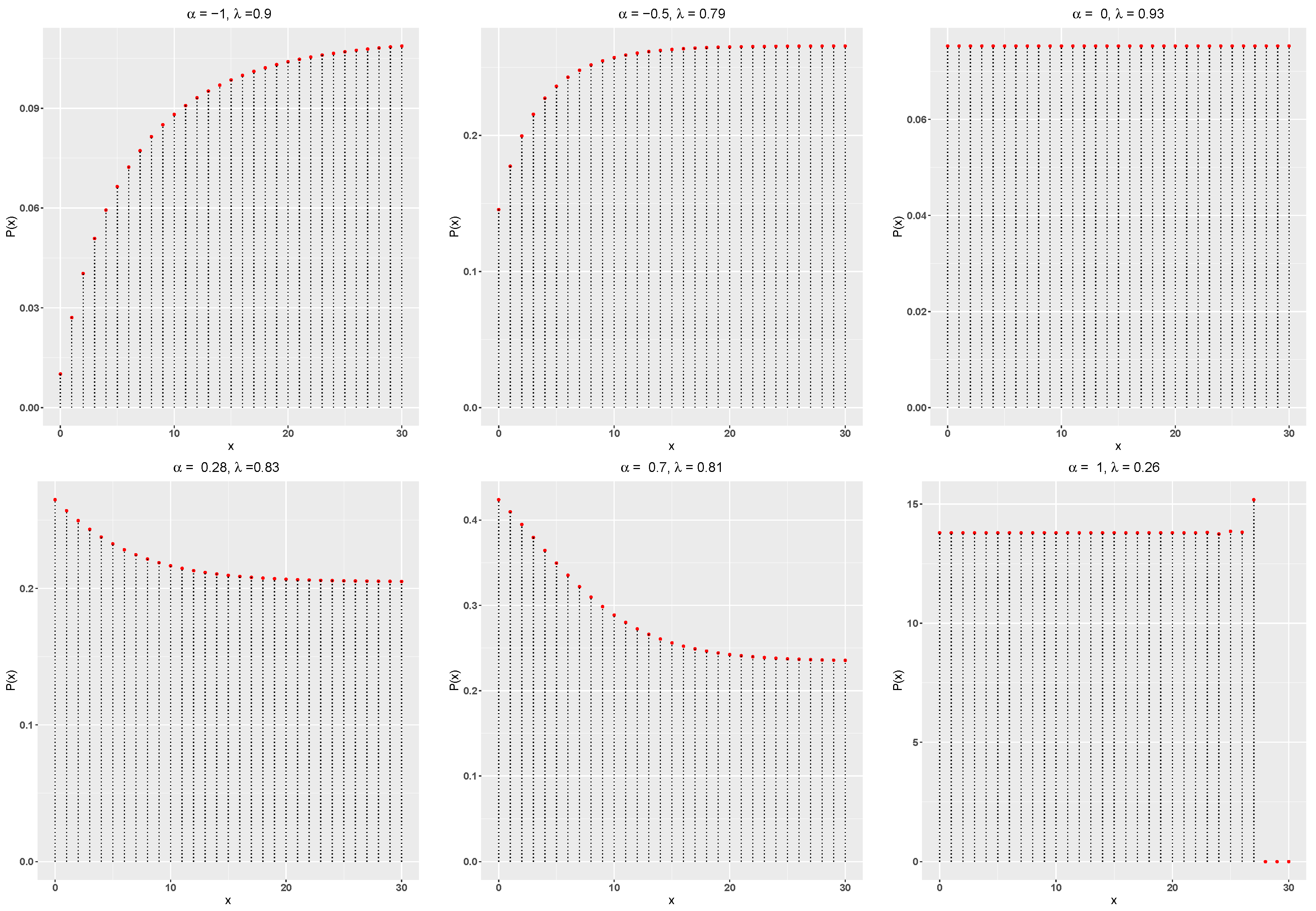
Figure 3.
Skewness (a) and kurtosis (b) of the DME distribution for different parameter values.
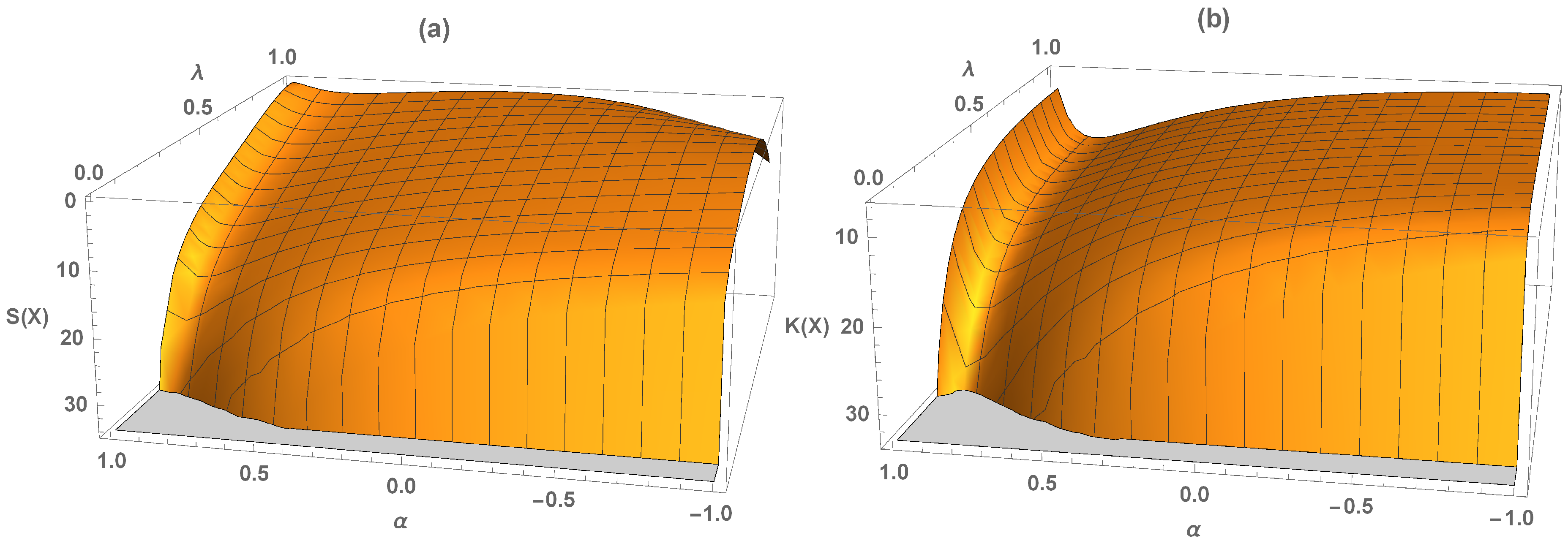
Figure 4.
DI of the DME distribution for different parameter values.
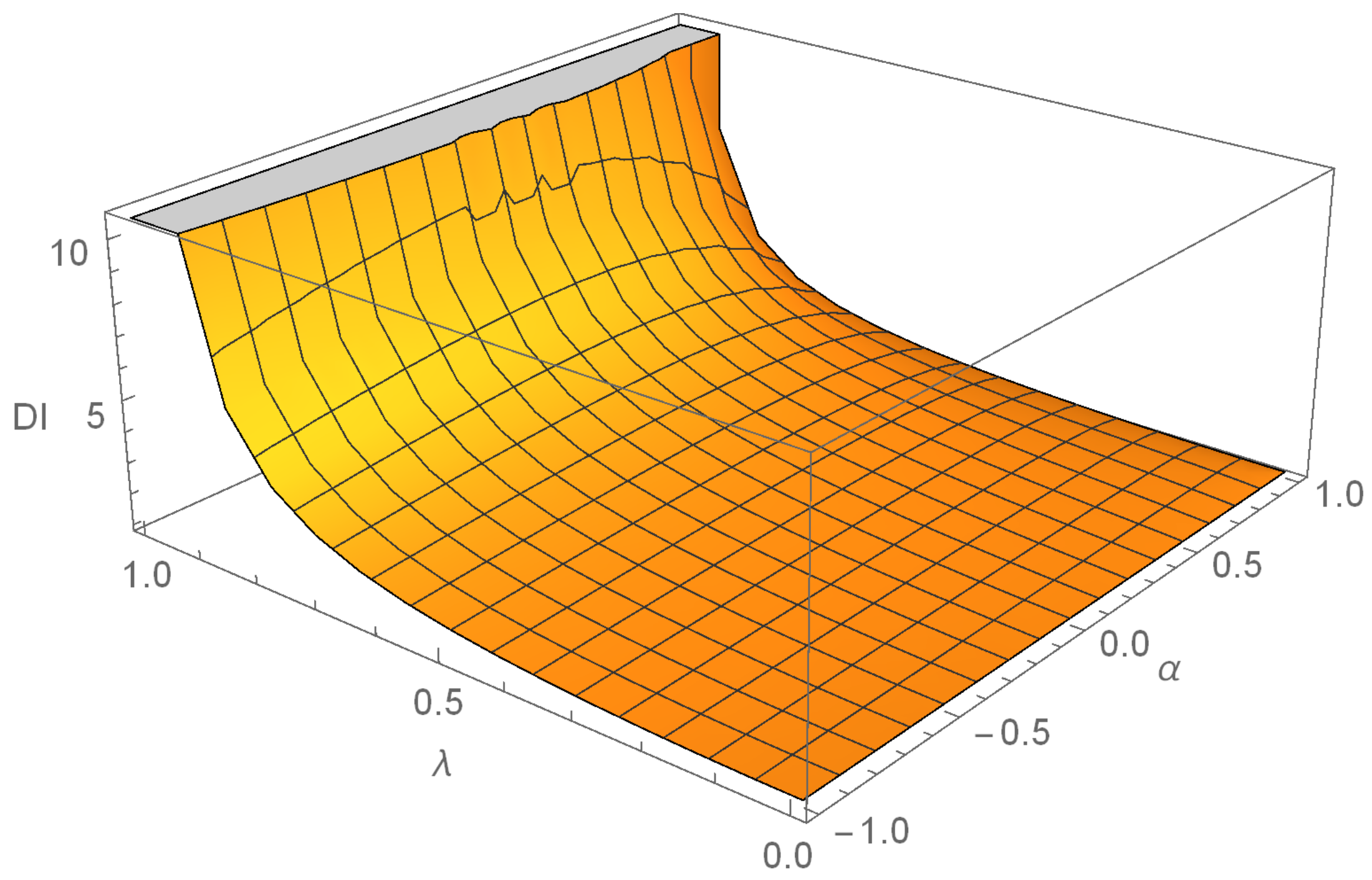
Figure 5.
Fitted pmfs of the various distributions for corn-borer data.
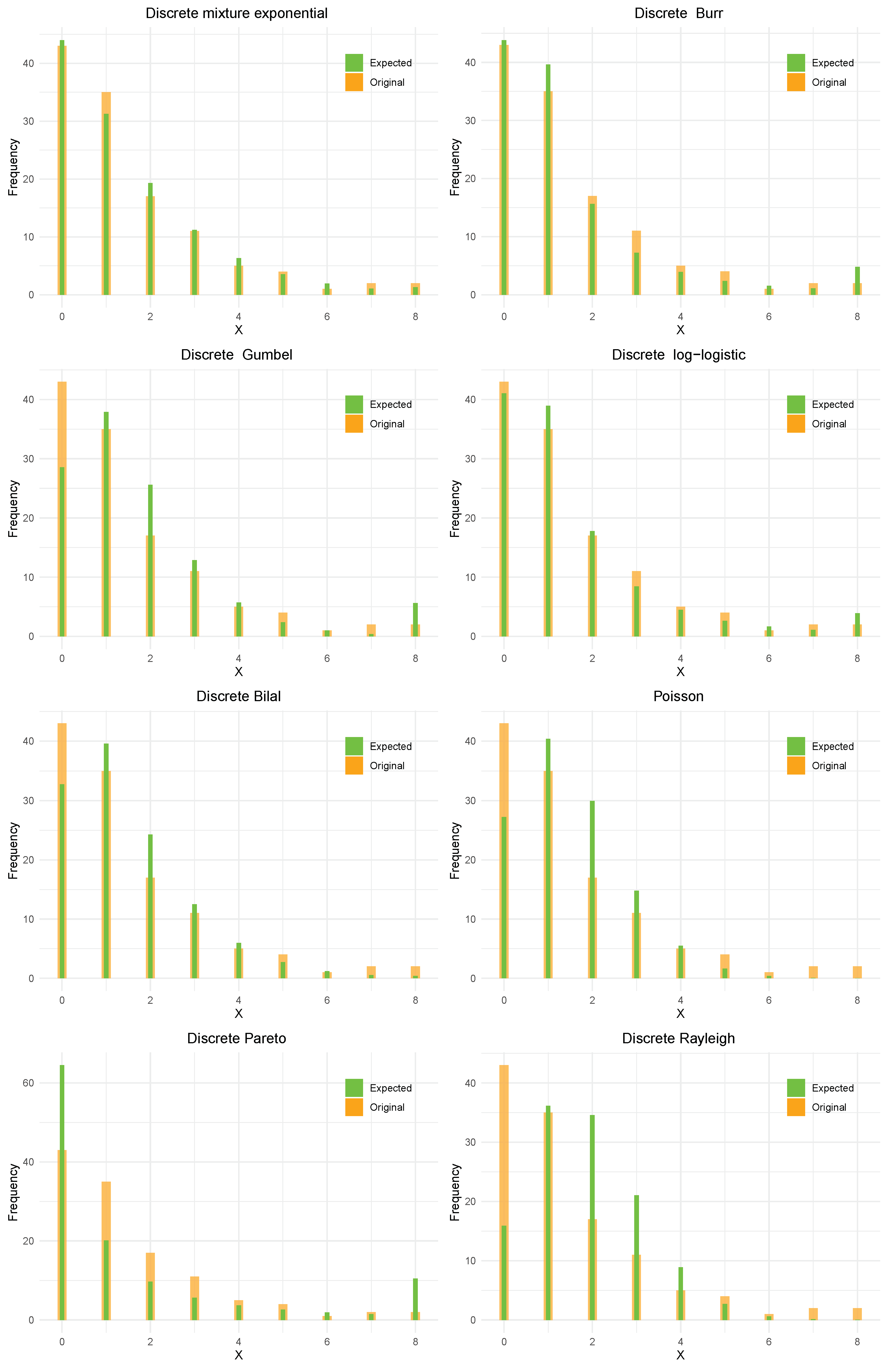
Figure 6.
The time series plot of the disorderly conduct data set.
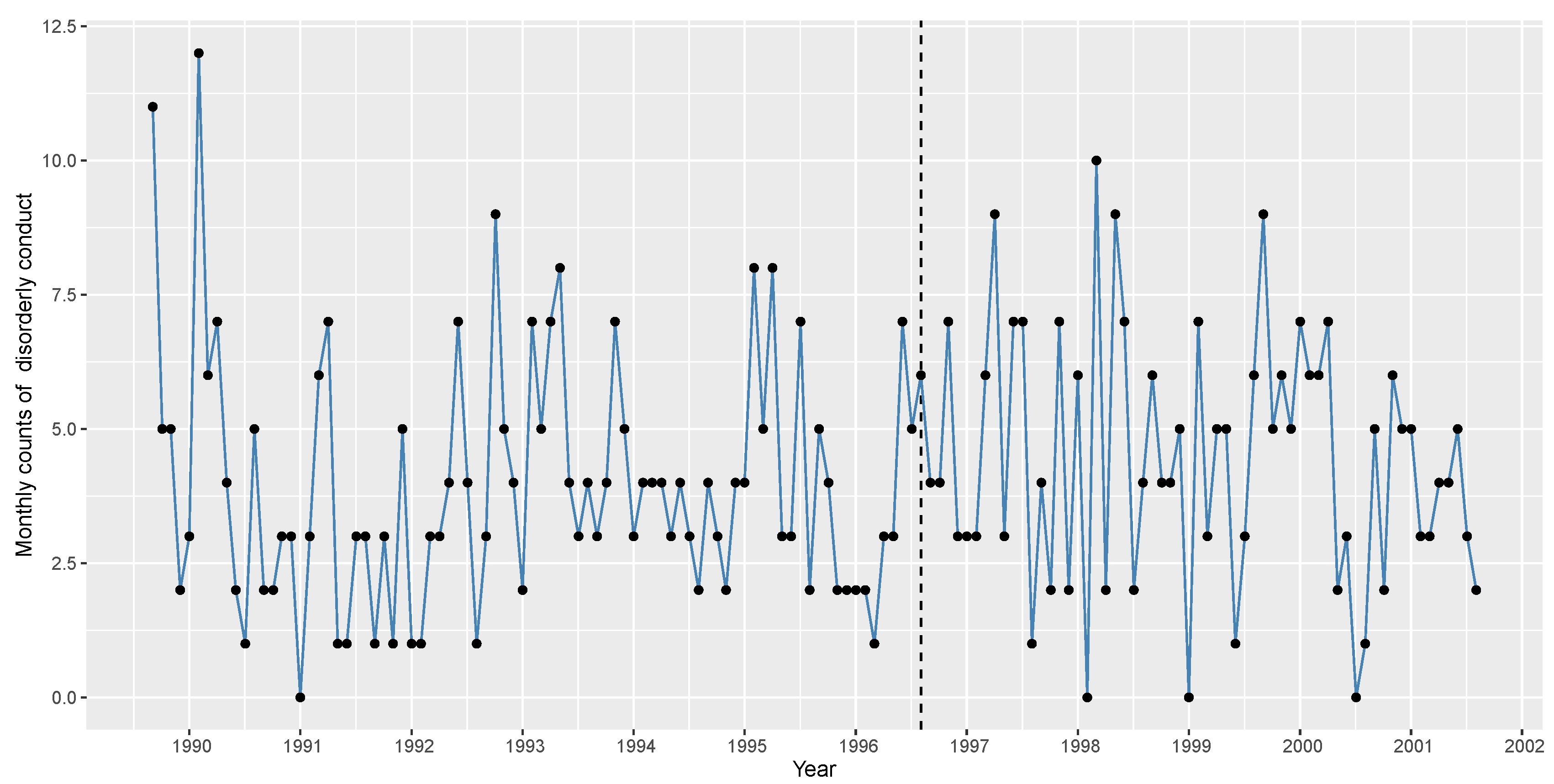
Figure 7.
The ACF (a) and PACF (b) plot of the Phase I data set.
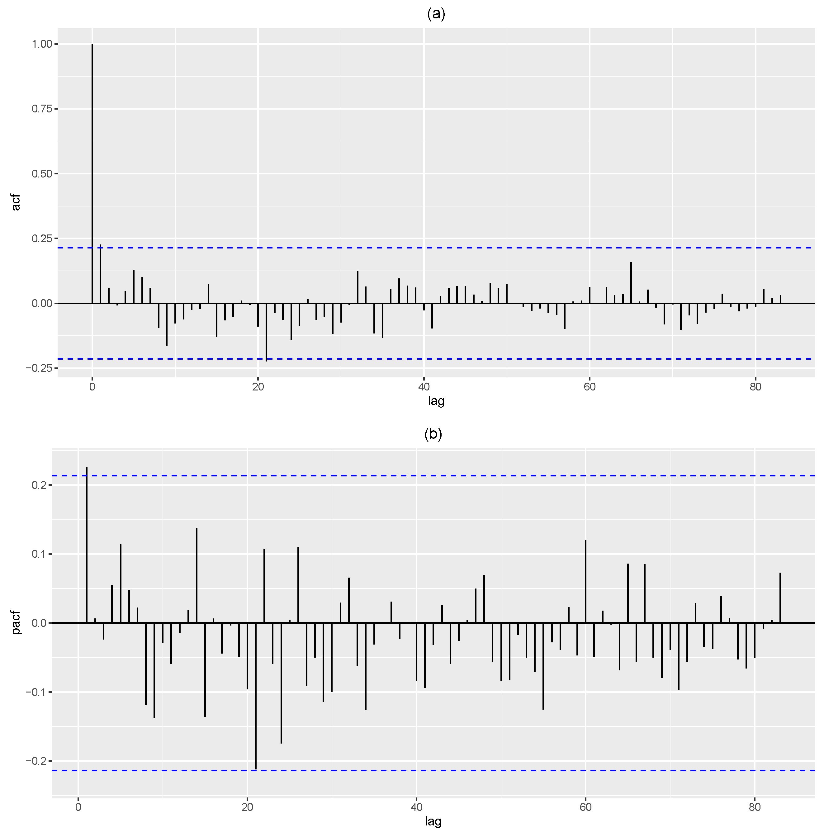
Figure 8.
The ACF plot of the Pearson residuals of the phase I data set.
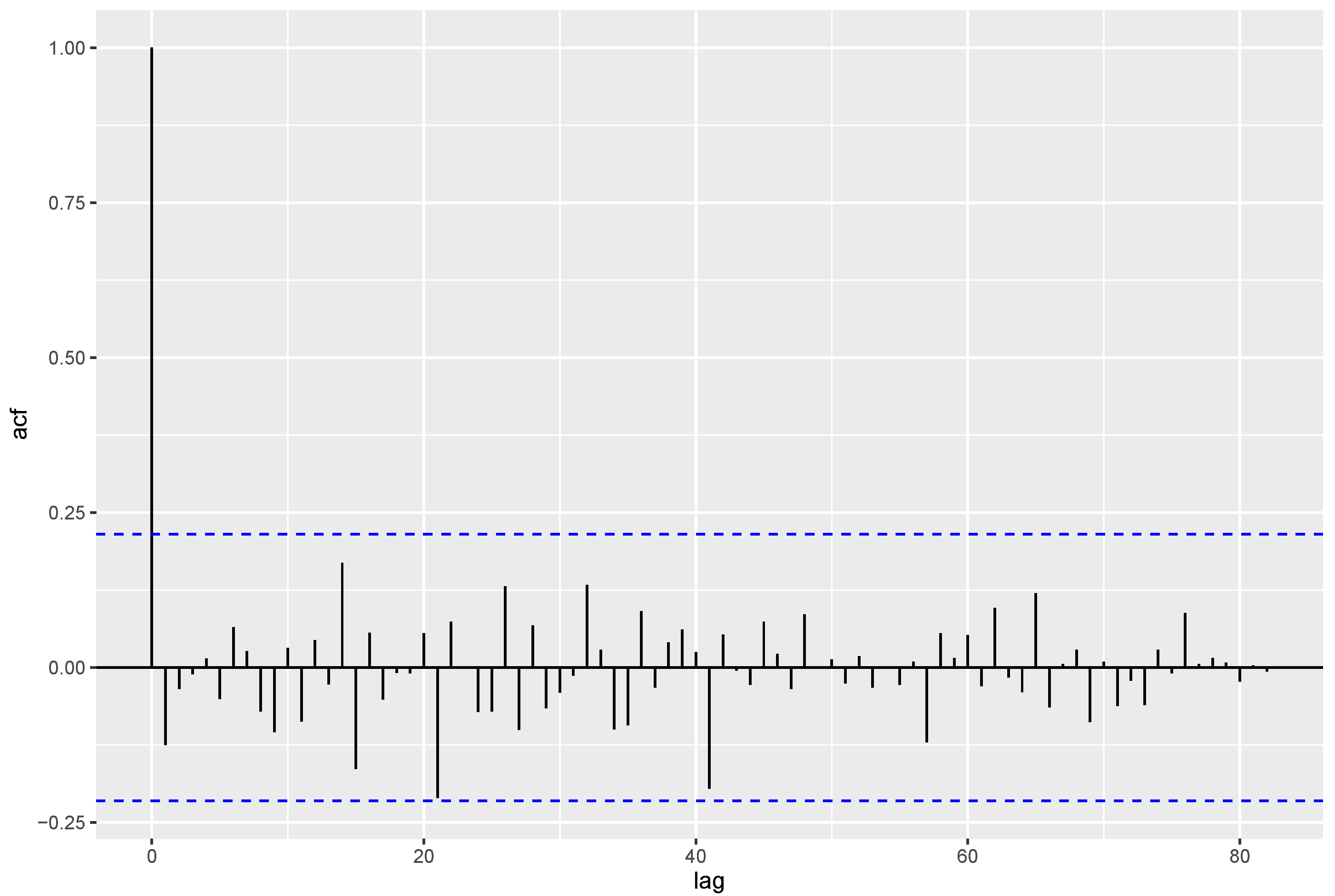
Figure 9.
The cpgrams of Pearson residuals of the phase I data set.
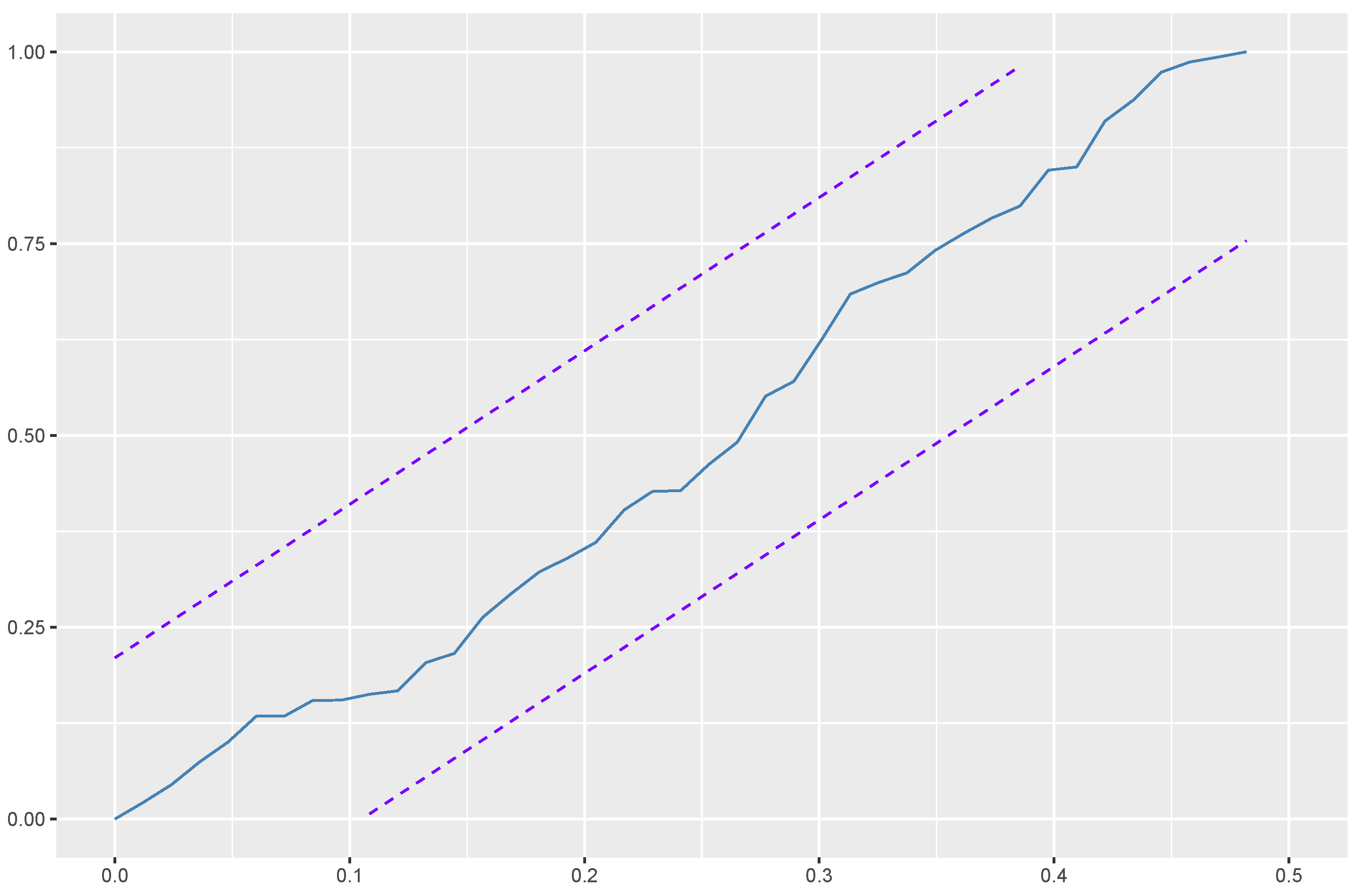
Figure 10.
The predicted versus the original values of the monthly counts of disorderly conduct (phase I) data.
Figure 10.
The predicted versus the original values of the monthly counts of disorderly conduct (phase I) data.
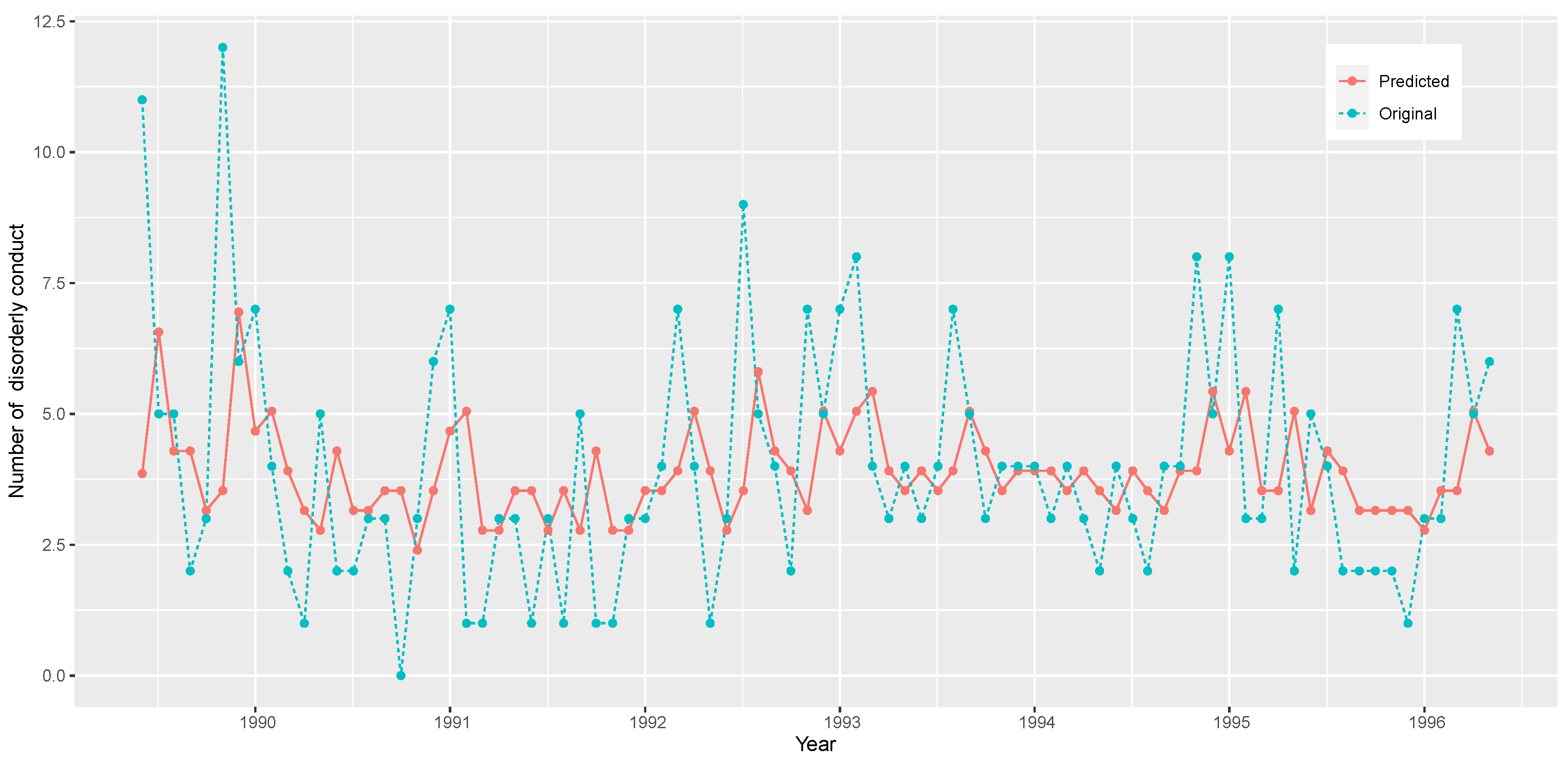
Figure 11.
The CUSUM plot of the monthly counts of disorderly conduct data.
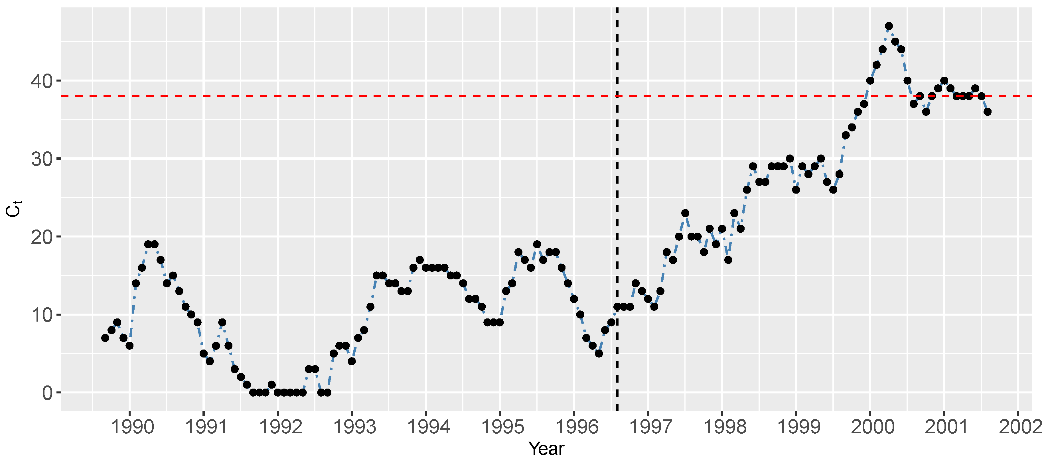

Table 1.
The mean, variance, DI, skewness and kurtosis of the discrete mixture exponential distribution.
Table 1.
The mean, variance, DI, skewness and kurtosis of the discrete mixture exponential distribution.
| DI | S(x) | K(x) | DI | S(x) | K(x) | |||||||
| 0.2 | 0.46 | 0.49 | 1.08 | 5.77 | 6.99 | 0.2 | 0.40 | 0.45 | 1.13 | 6.69 | 7.93 | |
| 0.5 | 1.67 | 2.67 | 1.60 | 0.51 | 6.88 | 0.5 | 1.47 | 2.56 | 1.75 | 1.38 | 7.22 | |
| 0.7 | 3.71 | 9.90 | 2.67 | 0.63 | 7.01 | 0.7 | 3.29 | 9.66 | 2.93 | 0.00 | 7.22 | |
| 0.8 | 6.22 | 25.19 | 4.05 | 2.55 | 7.05 | 0.8 | 5.56 | 24.67 | 4.44 | 0.42 | 7.22 | |
| 0.9 | 13.74 | 112.69 | 8.20 | 5.81 | 7.07 | 0.9 | 12.32 | 110.59 | 8.98 | 1.70 | 7.23 | |
| DI | S(x) | K(x) | DI | S(x) | K(x) | |||||||
| 0.2 | 0.33 | 0.40 | 1.19 | 7.91 | 9.28 | 0.2 | 0.25 | 0.31 | 1.25 | 10.37 | 12.20 | |
| 0.5 | 1.27 | 2.37 | 1.87 | 2.52 | 7.89 | 0.5 | 1.00 | 2.00 | 2.00 | 4.50 | 9.50 | |
| 0.7 | 2.88 | 9.08 | 3.15 | 0.40 | 7.75 | 0.7 | 2.33 | 7.78 | 3.33 | 1.86 | 9.13 | |
| 0.8 | 4.89 | 23.26 | 4.76 | 0.01 | 7.72 | 0.8 | 4.00 | 20.00 | 5.00 | 0.88 | 9.05 | |
| 0.9 | 10.89 | 104.46 | 9.59 | 0.19 | 7.71 | 0.9 | 9.00 | 90.00 | 10.00 | 0.24 | 9.01 | |
| DI | S(x) | K(x) | DI | S(x) | K(x) | |||||||
| 0.2 | 0.23 | 0.29 | 1.26 | 11.23 | 13.26 | 0.2 | 0.17 | 0.22 | 1.29 | 14.96 | 17.97 | |
| 0.5 | 0.93 | 1.88 | 2.02 | 5.11 | 10.09 | 0.5 | 0.73 | 1.48 | 2.02 | 7.39 | 12.59 | |
| 0.7 | 2.20 | 7.36 | 3.35 | 2.36 | 9.65 | 0.7 | 1.78 | 5.87 | 3.29 | 4.25 | 11.81 | |
| 0.8 | 3.78 | 18.94 | 5.01 | 1.28 | 9.55 | 0.8 | 3.11 | 15.16 | 4.87 | 2.85 | 11.65 | |
| 0.9 | 8.53 | 85.26 | 10.00 | 0.48 | 9.50 | 0.9 | 7.11 | 68.36 | 9.62 | 1.62 | 11.57 | |
| DI | S(x) | K(x) | DI | S(x) | K(x) | |||||||
| 0.2 | 0.10 | 0.13 | 1.28 | 22.18 | 27.39 | 0.2 | 0.04 | 0.04 | 1.04 | 31.00 | 32.04 | |
| 0.5 | 0.33 | 0.54 | 1.62 | 12.82 | 18.22 | 0.5 | 0.33 | 0.44 | 1.33 | 9.00 | 11.25 | |
| 0.7 | 1.37 | 4.05 | 2.95 | 6.64 | 15.16 | 0.7 | 0.96 | 1.88 | 1.96 | 4.65 | 9.53 | |
| 0.8 | 2.44 | 10.49 | 4.29 | 4.80 | 14.85 | 0.8 | 1.78 | 4.94 | 2.78 | 2.57 | 9.20 | |
| 0.9 | 5.68 | 47.42 | 8.34 | 3.05 | 14.70 | 0.9 | 4.26 | 22.44 | 5.26 | 0.80 | 9.04 | |
Table 2.
Simulation results of DME distribution.
| n | MLE | LSE | |||||||||||
| Estimate | Bias | RMSE | Estimate | Bias | RMSE | Estimate | Bias | RMSE | Estimate | Bias | RMSE | ||
| 100 | -0.966 | 0.034 | 0.066 | 0.901 | 0.006 | 0.007 | -0.972 | 0.028 | 0.063 | 0.906 | 0.007 | 0.009 | |
| 200 | -0.975 | 0.025 | 0.049 | 0.902 | 0.004 | 0.005 | -0.985 | 0.015 | 0.037 | 0.906 | 0.006 | 0.007 | |
| 300 | -0.983 | 0.017 | 0.033 | 0.902 | 0.003 | 0.004 | -0.993 | 0.007 | 0.021 | 0.905 | 0.006 | 0.006 | |
| 400 | -0.984 | 0.016 | 0.031 | 0.901 | 0.003 | 0.003 | -0.995 | 0.005 | 0.016 | 0.905 | 0.005 | 0.006 | |
| 500 | -0.985 | 0.015 | 0.027 | 0.902 | 0.002 | 0.003 | -0.997 | 0.003 | 0.012 | 0.905 | 0.005 | 0.006 | |
| 100 | -0.622 | 0.142 | 0.187 | 0.899 | 0.008 | 0.01 | -0.72 | 0.178 | 0.214 | 0.9 | 0.008 | 0.01 | |
| 200 | -0.617 | 0.094 | 0.134 | 0.9 | 0.005 | 0.007 | -0.737 | 0.161 | 0.187 | 0.9 | 0.005 | 0.007 | |
| 300 | -0.626 | 0.076 | 0.103 | 0.9 | 0.004 | 0.005 | -0.755 | 0.164 | 0.183 | 0.899 | 0.004 | 0.005 | |
| 400 | -0.622 | 0.062 | 0.083 | 0.9 | 0.003 | 0.004 | -0.751 | 0.155 | 0.17 | 0.9 | 0.003 | 0.004 | |
| 500 | -0.618 | 0.054 | 0.074 | 0.9 | 0.003 | 0.004 | -0.749 | 0.153 | 0.166 | 0.899 | 0.003 | 0.004 | |
| 100 | 0.188 | 0.295 | 0.357 | 0.722 | 0.043 | 0.053 | -0.791 | 1.041 | 1.053 | 0.64 | 0.09 | 0.098 | |
| 200 | 0.236 | 0.248 | 0.304 | 0.727 | 0.035 | 0.043 | -0.813 | 1.063 | 1.069 | 0.635 | 0.095 | 0.099 | |
| 300 | 0.266 | 0.225 | 0.28 | 0.732 | 0.032 | 0.04 | -0.823 | 1.073 | 1.077 | 0.634 | 0.096 | 0.099 | |
| 400 | 0.264 | 0.193 | 0.245 | 0.732 | 0.027 | 0.035 | -0.82 | 1.07 | 1.073 | 0.634 | 0.096 | 0.097 | |
| 500 | 0.267 | 0.177 | 0.229 | 0.732 | 0.026 | 0.033 | -0.824 | 1.074 | 1.077 | 0.634 | 0.096 | 0.098 | |
| 100 | 0.347 | 0.301 | 0.388 | 0.779 | 0.04 | 0.051 | -0.597 | 1.154 | 1.178 | 0.698 | 0.109 | 0.115 | |
| 200 | 0.41 | 0.249 | 0.308 | 0.788 | 0.032 | 0.04 | -0.702 | 1.208 | 1.216 | 0.685 | 0.116 | 0.119 | |
| 300 | 0.435 | 0.227 | 0.28 | 0.791 | 0.029 | 0.036 | -0.713 | 1.215 | 1.22 | 0.683 | 0.117 | 0.119 | |
| 400 | 0.45 | 0.214 | 0.261 | 0.793 | 0.026 | 0.032 | -0.718 | 1.218 | 1.221 | 0.683 | 0.117 | 0.118 | |
| 500 | 0.456 | 0.187 | 0.229 | 0.794 | 0.024 | 0.029 | -0.716 | 1.216 | 1.218 | 0.683 | 0.117 | 0.118 | |
| n | ADE | CVE | |||||||||||
| Estimate | Bias | RMSE | Estimate | Bias | RMSE | Estimate | Bias | RMSE | Estimate | Bias | RMSE | ||
| 100 | 0.432 | 1.432 | 1.432 | 0.974 | 0.074 | 0.074 | -0.98 | 0.02 | 0.051 | 0.905 | 0.007 | 0.008 | |
| 200 | 0.434 | 1.434 | 1.435 | 0.975 | 0.075 | 0.075 | -0.988 | 0.012 | 0.032 | 0.905 | 0.006 | 0.007 | |
| 300 | 0.434 | 1.434 | 1.434 | 0.975 | 0.075 | 0.075 | -0.994 | 0.006 | 0.019 | 0.905 | 0.006 | 0.006 | |
| 400 | 0.436 | 1.436 | 1.436 | 0.975 | 0.075 | 0.075 | -0.996 | 0.004 | 0.014 | 0.905 | 0.005 | 0.006 | |
| 500 | 0.436 | 1.436 | 1.436 | 0.975 | 0.075 | 0.075 | -0.997 | 0.003 | 0.011 | 0.905 | 0.005 | 0.006 | |
| 100 | 0.436 | 1.036 | 1.036 | 0.971 | 0.071 | 0.071 | -0.751 | 0.194 | 0.228 | 0.899 | 0.008 | 0.01 | |
| 200 | 0.437 | 1.037 | 1.037 | 0.972 | 0.072 | 0.072 | -0.754 | 0.174 | 0.198 | 0.899 | 0.005 | 0.007 | |
| 300 | 0.439 | 1.039 | 1.039 | 0.972 | 0.072 | 0.072 | -0.766 | 0.174 | 0.192 | 0.899 | 0.004 | 0.005 | |
| 400 | 0.439 | 1.039 | 1.039 | 0.972 | 0.072 | 0.072 | -0.759 | 0.162 | 0.178 | 0.899 | 0.003 | 0.004 | |
| 500 | 0.44 | 1.04 | 1.04 | 0.972 | 0.072 | 0.072 | -0.756 | 0.159 | 0.172 | 0.899 | 0.003 | 0.004 | |
| 100 | 0.451 | 0.201 | 0.202 | 0.894 | 0.164 | 0.164 | -0.82 | 1.07 | 1.081 | 0.636 | 0.095 | 0.102 | |
| 200 | 0.454 | 0.204 | 0.204 | 0.894 | 0.164 | 0.164 | -0.828 | 1.078 | 1.084 | 0.633 | 0.097 | 0.101 | |
| 300 | 0.455 | 0.205 | 0.205 | 0.894 | 0.164 | 0.164 | -0.834 | 1.084 | 1.087 | 0.632 | 0.098 | 0.1 | |
| 400 | 0.454 | 0.204 | 0.205 | 0.894 | 0.164 | 0.165 | -0.828 | 1.078 | 1.081 | 0.633 | 0.097 | 0.099 | |
| 500 | 0.455 | 0.205 | 0.205 | 0.894 | 0.164 | 0.164 | -0.831 | 1.081 | 1.083 | 0.633 | 0.097 | 0.099 | |
| 100 | 0.458 | 0.044 | 0.047 | 0.909 | 0.109 | 0.109 | -0.636 | 1.19 | 1.213 | 0.693 | 0.114 | 0.119 | |
| 200 | 0.461 | 0.039 | 0.042 | 0.91 | 0.11 | 0.11 | -0.721 | 1.227 | 1.234 | 0.682 | 0.118 | 0.121 | |
| 300 | 0.462 | 0.038 | 0.04 | 0.91 | 0.11 | 0.11 | -0.725 | 1.227 | 1.231 | 0.682 | 0.119 | 0.121 | |
| 400 | 0.462 | 0.038 | 0.04 | 0.91 | 0.11 | 0.111 | -0.727 | 1.227 | 1.23 | 0.682 | 0.118 | 0.12 | |
| 500 | 0.462 | 0.038 | 0.039 | 0.911 | 0.111 | 0.111 | -0.723 | 1.223 | 1.226 | 0.682 | 0.118 | 0.119 | |
Table 3.
MLEs with SEs and 95% CI, information criteria and goodness-of-fit-measures for the various distributions for corn-borer data.
Table 3.
MLEs with SEs and 95% CI, information criteria and goodness-of-fit-measures for the various distributions for corn-borer data.
| Distribution | Estimate | 95 % CI | log L | AIC | BIC | df | p-value | ||||
|---|---|---|---|---|---|---|---|---|---|---|---|
| lower bound | upper bound | ||||||||||
| DME | -0.3445 | 0.2925 | -0.9179 | 0.2288 | -200.3219 | 404.6439 | 410.2189 | 1.1878 | 3 | 0.7559 | |
| 0.5479 | 0.0476 | 0.4545 | 0.6412 | ||||||||
| DB | 2.3575 | 0.3656 | 1.6409 | 3.0742 | -204.2933 | 412.5865 | 418.1615 | 4.6477 | 3 | 0.1995 | |
| 0.519 | 0.0508 | 0.4194 | 0.6187 | ||||||||
| DG | 3.11 | 0.3674 | 2.39 | 3.8301 | -213.1911 | 430.3822 | 435.9572 | 10.801 | 3 | 0.0129 | |
| p | 0.4065 | 0.0294 | 0.3489 | 0.464 | |||||||
| DLL | 1.4007 | 0.1212 | 1.1631 | 1.6383 | -202.6303 | 409.2606 | 414.8356 | 2.2441 | 3 | 0.5233 | |
| 1.9429 | 0.1879 | 1.5746 | 2.3113 | ||||||||
| DBL | p | 0.6566 | 0.0186 | 0.6202 | 0.693 | -204.6753 | 411.3505 | 414.138 | 6.9961 | 3 | 0.072 |
| DP | 1.4833 | 0.1112 | 1.2654 | 1.7012 | -219.1879 | 440.3759 | 443.1634 | 21.761 | 3 | 0.0001 | |
| DPR | 0.3292 | 0.0338 | 0.2629 | 0.3954 | -220.6182 | 443.2363 | 446.0238 | 35.501 | 4 | 0 | |
| DR | 0.8673 | 0.0115 | 0.8448 | 0.8899 | -235.2266 | 472.4531 | 475.2406 | 60.054 | 3 | 0 | |
Table 4.
Observed and expected frequencies of corn-borer data under various distributions.
| Observed | DME | DB | DG | DLL | DBL | DP | DPR | DR |
|---|---|---|---|---|---|---|---|---|
| 43 | 44.01 | 43.83 | 28.54 | 41.03 | 32.74 | 27.23 | 64.45 | 15.92 |
| 35 | 31.28 | 39.61 | 37.88 | 38.94 | 39.59 | 40.38 | 20.15 | 36.17 |
| 17 | 19.29 | 15.62 | 25.60 | 17.77 | 24.28 | 29.95 | 9.69 | 34.58 |
| 11 | 11.21 | 7.21 | 12.85 | 8.43 | 12.51 | 14.81 | 5.65 | 21.03 |
| 5 | 6.34 | 3.91 | 5.70 | 4.48 | 5.97 | 5.49 | 3.68 | 8.89 |
| 4 | 3.53 | 2.38 | 2.40 | 2.63 | 2.74 | 1.63 | 2.58 | 2.70 |
| 1 | 1.95 | 1.56 | 0.99 | 1.66 | 1.23 | 0.40 | 1.90 | 0.60 |
| 2 | 1.07 | 1.09 | 0.40 | 1.12 | 0.54 | 0.09 | 1.46 | 0.10 |
| 2 | 1.31 | 4.80 | 5.63 | 3.93 | 0.42 | 0.02 | 10.44 | 0.01 |
Table 5.
DI of for various parameter values.
| -0.1 | -0.5 | -0.9 | 0.9 | 0.7 | 0.3 | 0.1 | |
| 0.1 | 1.0734 | 1.0478 | 1.0209 | 1.0794 | 1.1046 | 1.0956 | 1.0851 |
| 0.2 | 1.1683 | 1.1217 | 1.0702 | 1.1339 | 1.1994 | 1.2034 | 1.1880 |
| 0.3 | 1.2927 | 1.2276 | 1.1520 | 1.2002 | 1.3061 | 1.3344 | 1.3179 |
| 0.4 | 1.4603 | 1.3777 | 1.2765 | 1.2925 | 1.4422 | 1.5040 | 1.4893 |
| 0.5 | 1.6964 | 1.5952 | 1.4643 | 1.4286 | 1.6310 | 1.7381 | 1.7279 |
| 0.6 | 2.0517 | 1.9279 | 1.7580 | 1.6409 | 1.9152 | 2.0869 | 2.0848 |
| 0.7 | 2.6449 | 2.4884 | 2.2594 | 2.0049 | 2.3922 | 2.6667 | 2.6789 |
| 0.8 | 3.8321 | 3.6156 | 3.2751 | 2.7460 | 3.3521 | 3.8254 | 3.8665 |
| 0.9 | 7.3947 | 7.0056 | 6.3410 | 4.9925 | 6.2444 | 7.3017 | 7.4286 |
| -0.1 | -0.5 | -0.9 | 0.9 | 0.7 | 0.3 | 0.1 | |
| 0.1 | 1.0604 | 1.0394 | 1.0172 | 1.0654 | 1.0862 | 1.0787 | 1.0701 |
| 0.2 | 1.1386 | 1.1002 | 1.0578 | 1.1103 | 1.1642 | 1.1675 | 1.1549 |
| 0.3 | 1.2410 | 1.1875 | 1.1252 | 1.1648 | 1.2521 | 1.2754 | 1.2618 |
| 0.4 | 1.3791 | 1.3111 | 1.2277 | 1.2409 | 1.3641 | 1.4151 | 1.4029 |
| 0.5 | 1.5735 | 1.4902 | 1.3824 | 1.3529 | 1.5196 | 1.6078 | 1.5994 |
| 0.6 | 1.8661 | 1.7642 | 1.6243 | 1.5278 | 1.7537 | 1.8951 | 1.8934 |
| 0.7 | 2.3546 | 2.2258 | 2.0372 | 1.8276 | 2.1465 | 2.3725 | 2.3826 |
| 0.8 | 3.3323 | 3.1540 | 2.8736 | 2.4379 | 2.9370 | 3.3268 | 3.3606 |
| 0.9 | 6.2663 | 5.9458 | 5.3985 | 4.2879 | 5.3189 | 6.1896 | 6.2941 |
Table 6.
Simulation results of INAR(1)DME process.
| n | CML | ||||||||
| p | |||||||||
| Estimate | Bias | RMSE | Estimate | Bias | RMSE | Estimate | Bias | RMSE | |
| 50 | 0.2871 | 0.0846 | 0.1052 | 0.7722 | 0.2279 | 0.2653 | 0.5865 | 0.0663 | 0.0828 |
| 100 | 0.2904 | 0.0588 | 0.0747 | 0.7692 | 0.2010 | 0.2414 | 0.5910 | 0.0554 | 0.0680 |
| 150 | 0.2942 | 0.0492 | 0.0611 | 0.7772 | 0.1899 | 0.2259 | 0.5935 | 0.0517 | 0.0632 |
| 200 | 0.2967 | 0.0410 | 0.0510 | 0.7781 | 0.1822 | 0.2193 | 0.5942 | 0.0496 | 0.0603 |
| 250 | 0.2924 | 0.0382 | 0.0477 | 0.7664 | 0.1834 | 0.2214 | 0.5939 | 0.0494 | 0.0599 |
| 50 | 0.4758 | 0.0915 | 0.1172 | 0.2044 | 0.2371 | 0.2690 | 0.3047 | 0.0650 | 0.0813 |
| 100 | 0.4884 | 0.0637 | 0.0814 | 0.2299 | 0.2385 | 0.2797 | 0.3089 | 0.0572 | 0.0735 |
| 150 | 0.4918 | 0.0513 | 0.0644 | 0.2329 | 0.2333 | 0.2797 | 0.3114 | 0.0536 | 0.0692 |
| 200 | 0.4953 | 0.0432 | 0.0544 | 0.2506 | 0.2312 | 0.2805 | 0.3159 | 0.0524 | 0.0683 |
| 250 | 0.4940 | 0.0393 | 0.0495 | 0.2448 | 0.2232 | 0.2726 | 0.3149 | 0.0498 | 0.0662 |
| 50 | 0.1953 | 0.0974 | 0.1180 | -0.5697 | 0.3821 | 0.4713 | 0.4088 | 0.0625 | 0.0798 |
| 100 | 0.1936 | 0.0716 | 0.0890 | -0.5881 | 0.3054 | 0.3810 | 0.4044 | 0.0438 | 0.0583 |
| 150 | 0.1958 | 0.0597 | 0.0738 | -0.6102 | 0.2715 | 0.3307 | 0.4017 | 0.0376 | 0.0486 |
| 200 | 0.1996 | 0.0516 | 0.0642 | -0.6115 | 0.2352 | 0.2993 | 0.4013 | 0.0336 | 0.0454 |
| 250 | 0.1931 | 0.0470 | 0.0586 | -0.6213 | 0.2088 | 0.2525 | 0.4005 | 0.0284 | 0.0357 |
| 50 | 0.2832 | 0.0751 | 0.0937 | -0.4408 | 0.4310 | 0.5110 | 0.6982 | 0.0421 | 0.0543 |
| 100 | 0.2903 | 0.0539 | 0.0680 | -0.4046 | 0.3253 | 0.4119 | 0.7022 | 0.0320 | 0.0416 |
| 150 | 0.2894 | 0.0456 | 0.0569 | -0.4420 | 0.2746 | 0.3495 | 0.6987 | 0.0265 | 0.0343 |
| 200 | 0.2948 | 0.0395 | 0.0501 | -0.4028 | 0.2448 | 0.3157 | 0.7006 | 0.0230 | 0.0309 |
| 250 | 0.2949 | 0.0358 | 0.0460 | -0.4116 | 0.2150 | 0.2809 | 0.7004 | 0.0203 | 0.0272 |
| n | CLS | ||||||||
| p | |||||||||
| Estimate | Bias | RMSE | Estimate | Bias | RMSE | Estimate | Bias | RMSE | |
| 50 | 0.2634 | 0.1172 | 0.1441 | 0.8146 | 0.0293 | 0.0441 | 0.5345 | 0.0829 | 0.1056 |
| 100 | 0.2775 | 0.0853 | 0.1050 | 0.8197 | 0.0228 | 0.0293 | 0.5361 | 0.0709 | 0.0884 |
| 150 | 0.2888 | 0.0701 | 0.0868 | 0.8211 | 0.0225 | 0.0269 | 0.5322 | 0.0717 | 0.0848 |
| 200 | 0.2902 | 0.0603 | 0.0753 | 0.8213 | 0.0219 | 0.0260 | 0.5330 | 0.0692 | 0.0810 |
| 250 | 0.2911 | 0.0557 | 0.0696 | 0.8208 | 0.0212 | 0.0248 | 0.5341 | 0.0673 | 0.0779 |
| 50 | 0.4367 | 0.1233 | 0.1559 | 0.3668 | 0.1681 | 0.2312 | 0.2416 | 0.0879 | 0.1074 |
| 100 | 0.4643 | 0.0888 | 0.1107 | 0.3308 | 0.1309 | 0.1637 | 0.2187 | 0.0899 | 0.1059 |
| 150 | 0.4779 | 0.0697 | 0.0885 | 0.3188 | 0.1189 | 0.1349 | 0.2094 | 0.0932 | 0.1056 |
| 200 | 0.4872 | 0.0584 | 0.0736 | 0.3115 | 0.1115 | 0.1185 | 0.2040 | 0.0970 | 0.1063 |
| 250 | 0.4858 | 0.0560 | 0.0703 | 0.3121 | 0.1121 | 0.1175 | 0.2048 | 0.0961 | 0.1051 |
| 50 | 0.1769 | 0.1096 | 0.1312 | -0.4702 | 0.1469 | 0.1861 | 0.3708 | 0.0613 | 0.0769 |
| 100 | 0.1851 | 0.0861 | 0.1048 | -0.4690 | 0.1376 | 0.1646 | 0.3663 | 0.0519 | 0.0645 |
| 150 | 0.1901 | 0.0679 | 0.0849 | -0.4698 | 0.1348 | 0.1541 | 0.3654 | 0.0458 | 0.0565 |
| 200 | 0.1949 | 0.0591 | 0.0740 | -0.4717 | 0.1299 | 0.1469 | 0.3639 | 0.0436 | 0.0534 |
| 250 | 0.1905 | 0.0555 | 0.0696 | -0.4734 | 0.1277 | 0.1423 | 0.3657 | 0.0407 | 0.0499 |
| 50 | 0.2579 | 0.1103 | 0.1367 | -0.2817 | 0.1197 | 0.1484 | 0.6446 | 0.0757 | 0.0981 |
| 100 | 0.2824 | 0.0789 | 0.0981 | -0.2804 | 0.1199 | 0.1360 | 0.6367 | 0.0702 | 0.0872 |
| 150 | 0.2871 | 0.0616 | 0.0762 | -0.2819 | 0.1182 | 0.1285 | 0.6360 | 0.0666 | 0.0794 |
| 200 | 0.2924 | 0.0591 | 0.0739 | -0.2785 | 0.1215 | 0.1309 | 0.6329 | 0.0689 | 0.0815 |
| 250 | 0.2932 | 0.0509 | 0.0640 | -0.2809 | 0.1191 | 0.1263 | 0.6338 | 0.0672 | 0.0773 |
Table 7.
Mean of of INAR(1)DME process.
| -0.1 | -0.3 | -0.5 | -0.7 | -0.9 | 0.9 | 0.7 | 0.5 | 0.3 | 0.1 | |
| 0.1 | 0.202 | 0.236 | 0.269 | 0.303 | 0.337 | 0.034 | 0.067 | 0.101 | 0.135 | 0.168 |
| 0.2 | 0.451 | 0.521 | 0.59 | 0.66 | 0.729 | 0.104 | 0.174 | 0.243 | 0.312 | 0.382 |
| 0.3 | 0.769 | 0.879 | 0.989 | 1.099 | 1.209 | 0.22 | 0.33 | 0.44 | 0.549 | 0.659 |
| 0.4 | 1.19 | 1.349 | 1.508 | 1.667 | 1.825 | 0.397 | 0.556 | 0.714 | 0.873 | 1.032 |
| 0.5 | 1.778 | 2 | 2.222 | 2.444 | 2.667 | 0.667 | 0.889 | 1.111 | 1.333 | 1.556 |
| 0.6 | 2.656 | 2.969 | 3.281 | 3.594 | 3.906 | 1.094 | 1.406 | 1.719 | 2.031 | 2.344 |
| 0.7 | 4.118 | 4.575 | 5.033 | 5.49 | 5.948 | 1.83 | 2.288 | 2.745 | 3.203 | 3.66 |
| 0.8 | 7.037 | 7.778 | 8.519 | 9.259 | 10 | 3.333 | 4.074 | 4.815 | 5.556 | 6.296 |
| 0.9 | 15.789 | 17.368 | 18.947 | 20.526 | 22.105 | 7.895 | 9.474 | 11.053 | 12.632 | 14.211 |
| -0.1 | -0.3 | -0.5 | -0.7 | -0.9 | 0.9 | 0.7 | 0.5 | 0.3 | 0.1 | |
| 0.1 | 0.404 | 0.471 | 0.539 | 0.606 | 0.673 | 0.067 | 0.135 | 0.202 | 0.269 | 0.337 |
| 0.2 | 0.903 | 1.042 | 1.181 | 1.319 | 1.458 | 0.208 | 0.347 | 0.486 | 0.625 | 0.764 |
| 0.3 | 1.538 | 1.758 | 1.978 | 2.198 | 2.418 | 0.44 | 0.659 | 0.879 | 1.099 | 1.319 |
| 0.4 | 2.381 | 2.698 | 3.016 | 3.333 | 3.651 | 0.794 | 1.111 | 1.429 | 1.746 | 2.063 |
| 0.5 | 3.556 | 4 | 4.444 | 4.889 | 5.333 | 1.333 | 1.778 | 2.222 | 2.667 | 3.111 |
| 0.6 | 5.312 | 5.937 | 6.562 | 7.187 | 7.812 | 2.187 | 2.812 | 3.437 | 4.062 | 4.687 |
| 0.7 | 8.235 | 9.15 | 10.065 | 10.98 | 11.895 | 3.66 | 4.575 | 5.49 | 6.405 | 7.32 |
| 0.8 | 14.074 | 15.556 | 17.037 | 18.519 | 20 | 6.667 | 8.148 | 9.63 | 11.111 | 12.593 |
Table 8.
Deviations of mean of INAR(1)DME process with in-control values of .
| and | and | |||||||||||
| -0.1 | -0.3 | -0.5 | -0.7 | -0.9 | 0.9 | 0.7 | 0.5 | 0.3 | 0.1 | |||
| 0.4 | 1.19 | 1.349 | 1.508 | 1.667 | 1.825 | 0.4 | 0.794 | 1.111 | 1.429 | 1.746 | 2.063 | |
| (13.36%) | (26.72%) | (40.08%) | (53.36%) | (39.92%) | (79.97%) | (119.90%) | (159.82%) | |||||
| 0.49 | 1.709 | 1.924 | 2.139 | 2.354 | 2.569 | 0.49 | 1.268 | 1.698 | 2.128 | 2.558 | 2.988 | |
| (12.58%) | (25.16%) | (37.74%) | (50.32%) | (33.91%) | (67.82%) | (101.74%) | (135.65%) | |||||
| 0.6 | 2.656 | 2.969 | 3.281 | 3.594 | 3.906 | 0.6 | 2.187 | 2.812 | 3.437 | 4.062 | 4.687 | |
| (11.78%) | (23.53%) | (35.32%) | (47.06%) | (28.58%) | (57.16%) | (85.73%) | (114.31%) | |||||
| 0.65 | 3.283 | 3.658 | 4.033 | 4.408 | 4.784 | 0.65 | 2.814 | 3.564 | 4.315 | 5.065 | 5.815 | |
| (11.42%) | (22.84%) | (34.27%) | (45.72%) | (26.65%) | (53.34%) | (79.99%) | (106.65%) | |||||
| 0.77 | 5.895 | 6.525 | 7.156 | 7.786 | 8.417 | 0.77 | 5.485 | 6.746 | 8.007 | 9.268 | 10.529 | |
| (10.69%) | (21.39%) | (32.08%) | (42.78%) | (22.99%) | (45.98%) | (68.97%) | (91.96%) | |||||
| 0.9 | 15.789 | 17.368 | 18.947 | 20.526 | 22.105 | 0.9 | 15.789 | 18.947 | 22.105 | 25.263 | 28.421 | |
| (10.00%) | (20.00%) | (30.00%) | (40.00%) | (20.00%) | (40.00%) | (60.00%) | (80.01%) | |||||
Table 9.
ARL with deviation (in parenthesis) for the CUSUM charts with and .
| k | h | ||||||||
|---|---|---|---|---|---|---|---|---|---|
| -0.1 | -0.3 | -0.5 | -0.7 | -0.9 | |||||
| 0.4 | 2 | 10 | 0 | 0.4 | 308.03 | 191.61 | 125.81 | 86.53 | 62.01 |
| (-37.80%) | (-59.16%) | (-71.91%) | (-79.87%) | ||||||
| 2 | 10 | 0 | 0.49 | 60.99 | 42.36 | 31.12 | 23.92 | 19.1 | |
| (-80.20%) | (-86.25%) | (-89.90%) | (-92.23%) | (-93.80%) | |||||
| 2 | 10 | 0 | 0.6 | 16.83 | 13.36 | 11.02 | 9.35 | 8.11 | |
| (-94.54%) | (-95.66%) | (-96.42%) | (-96.96%) | (-97.37%) | |||||
| 3 | 5 | 0 | 0.4 | 294.83 | 208.65 | 153 | 115.41 | 89.09 | |
| (-29.23%) | (-48.11%) | (-60.85%) | (-69.78%) | ||||||
| 3 | 5 | 0 | 0.49 | 67.89 | 50.25 | 38.51 | 30.34 | 24.46 | |
| (-76.97%) | (-82.96%) | (-86.94%) | (-89.71%) | (-91.70%) | |||||
| 3 | 5 | 0 | 0.6 | 17.97 | 14.26 | 11.65 | 9.76 | 8.33 | |
| (-93.90%) | (-95.16%) | (-96.05%) | (-96.69%) | (-97.17%) | |||||
| 2 | 10 | 4 | 0.4 | 300.25 | 184.7 | 119.6 | 80.89 | 56.85 | |
| (-38.48%) | (-60.17%) | (-73.06%) | (-81.07%) | ||||||
| 2 | 10 | 4 | 0.49 | 56.71 | 38.5 | 27.61 | 20.71 | 16.13 | |
| (-81.11%) | (-87.18%) | (-90.80%) | (-93.10%) | (-94.63%) | |||||
| 2 | 10 | 4 | 0.6 | 14.53 | 11.27 | 9.1 | 7.58 | 6.46 | |
| (-95.16%) | (-96.25%) | (-96.97%) | (-97.48%) | (-97.85%) | |||||
| 0.65 | 5 | 20 | 0 | 0.65 | 288.72 | 174.69 | 111.65 | 74.87 | 52.46 |
| (-39.50%) | (-61.33%) | (-74.07%) | (-81.83%) | ||||||
| 5 | 20 | 0 | 0.77 | 19.5 | 15.05 | 12.13 | 10.1 | 8.63 | |
| (-93.25%) | (-94.79%) | (-95.80%) | (-96.50%) | (-97.01%) | |||||
| 5 | 20 | 0 | 0.9 | 3.96 | 3.55 | 3.22 | 2.95 | 2.73 | |
| (-98.63%) | (-98.77%) | (-98.88%) | (-98.98%) | (-99.05%) | |||||
| 7 | 11 | 0 | 0.65 | 309.75 | 215.68 | 155.5 | 115.27 | 87.42 | |
| (-30.37%) | (-49.80%) | (-62.79%) | (-71.78%) | ||||||
| 7 | 11 | 0 | 0.77 | 22.56 | 17.46 | 13.96 | 11.46 | 9.61 | |
| (-92.72%) | (-94.36%) | (-95.49%) | (-96.30%) | (-96.90%) | |||||
| 7 | 11 | 0 | 0.9 | 3.58 | 3.17 | 2.85 | 2.58 | 2.37 | |
| (-98.84%) | (-98.98%) | (-99.08%) | (-99.17%) | (-99.23%) | |||||
| 7 | 11 | 4 | 0.65 | 307.21 | 213.37 | 153.39 | 113.33 | 85.62 | |
| (-30.55%) | (-50.07%) | (-63.11%) | (-72.13%) | ||||||
| 7 | 11 | 4 | 0.77 | 21.61 | 16.57 | 13.13 | 10.66 | 8.85 | |
| (-92.97%) | (-94.61%) | (-95.73%) | (-96.53%) | (-97.12%) | |||||
| 7 | 11 | 4 | 0.9 | 3.25 | 2.85 | 2.54 | 2.29 | 2.08 | |
| (-98.94%) | (-99.07%) | (-99.17%) | (-99.25%) | (-99.32%) | |||||
Table 10.
ARL with deviation (in parenthesis) for the CUSUM charts with and .
| k | h | ||||||||
|---|---|---|---|---|---|---|---|---|---|
| 0.9 | 0.7 | 0.5 | 0.3 | 0.1 | |||||
| 0.4 | 1 | 5 | 0 | 0.4 | 320.07 | 112.44 | 60.28 | 38.46 | 27.12 |
| (-64.87%) | (-81.17%) | (-87.98%) | (-91.53%) | ||||||
| 1 | 5 | 0 | 0.49 | 86.79 | 39.97 | 24.74 | 17.5 | 13.37 | |
| (-72.88%) | (-87.51%) | (-92.27%) | (-94.53%) | (-95.82%) | |||||
| 1 | 5 | 0 | 0.6 | 24.1 | 15.05 | 10.92 | 8.57 | 7.06 | |
| (-92.47%) | (-95.30%) | (-96.59%) | (-97.32%) | (-97.79%) | |||||
| 1 | 5 | 2 | 0.4 | 315.34 | 109.18 | 57.59 | 36.1 | 24.99 | |
| (-65.38%) | (-81.74%) | (-88.55%) | (-92.08%) | ||||||
| 1 | 5 | 2 | 0.49 | 83.67 | 37.72 | 22.86 | 15.84 | 11.88 | |
| (-73.47%) | (-88.04%) | (-92.75%) | (-94.98%) | (-96.23%) | |||||
| 1 | 5 | 2 | 0.6 | 22.16 | 13.58 | 9.68 | 7.48 | 6.08 | |
| (-92.97%) | (-95.69%) | (-96.93%) | (-97.63%) | (-98.07%) | |||||
| 1 | 5 | 4 | 0.4 | 297.06 | 98.92 | 50.15 | 30.23 | 20.17 | |
| (-66.70%) | (-83.12%) | (-89.82%) | (-93.21%) | ||||||
| 1 | 5 | 4 | 0.49 | 74.35 | 32.01 | 18.62 | 12.46 | 9.06 | |
| (-74.97%) | (-89.22%) | (-93.73%) | (-95.81%) | (-96.95%) | |||||
| 1 | 5 | 4 | 0.6 | 17.85 | 10.63 | 7.41 | 5.63 | 4.51 | |
| (-93.99%) | (-96.42%) | (-97.51%) | (-98.10%) | (-98.48%) | |||||
| 0.65 | 2 | 16 | 0 | 0.65 | 286.98 | 87.72 | 44.66 | 28.34 | 20.34 |
| (-69.43%) | (-84.44%) | (-90.12%) | (-92.91%) | ||||||
| 2 | 16 | 0 | 0.77 | 23.6 | 15.37 | 11.46 | 9.18 | 7.68 | |
| (-91.78%) | (-94.64%) | (-96.01%) | (-96.80%) | (-97.32%) | |||||
| 2 | 16 | 0 | 0.9 | 5.03 | 4.35 | 3.83 | 3.42 | 3.09 | |
| (-98.25%) | (-98.48%) | (-98.67%) | (-98.81%) | (-98.92%) | |||||
| 3 | 9 | 0 | 0.65 | 292.12 | 99.56 | 53.06 | 33.69 | 23.63 | |
| (-65.92%) | (-81.84%) | (-88.47%) | (-91.91%) | ||||||
| 3 | 9 | 0 | 0.77 | 27.81 | 16.35 | 11.49 | 8.82 | 7.15 | |
| (-90.48%) | (-94.40%) | (-96.07%) | (-96.98%) | (-97.55%) | |||||
| 3 | 9 | 0 | 0.9 | 4.41 | 3.77 | 3.29 | 2.92 | 2.62 | |
| (-98.49%) | (-98.71%) | (-98.87%) | (-99.00%) | (-99.10%) | |||||
| 4 | 6 | 4 | 0.65 | 308.87 | 106.7 | 57.88 | 36.99 | 25.83 | |
| (-65.46%) | (-81.26%) | (-88.02%) | (-91.64%) | ||||||
| 4 | 6 | 4 | 0.77 | 30.44 | 16.67 | 11.17 | 8.24 | 6.44 | |
| (-90.14%) | (-94.60%) | (-96.38%) | (-97.33%) | (-97.92%) | |||||
| 4 | 6 | 4 | 0.9 | 3.65 | 3.07 | 2.65 | 2.34 | 2.08 | |
| (-98.82%) | (-99.01%) | (-99.14%) | (-99.24%) | (-99.33%) | |||||
Table 11.
ARL with deviation (in parenthesis) for the EWMA charts with and having C chart with u = (7,14).
Table 11.
ARL with deviation (in parenthesis) for the EWMA charts with and having C chart with u = (7,14).
| l | u | |||||||||
|---|---|---|---|---|---|---|---|---|---|---|
| -0.1 | -0.3 | -0.5 | -0.7 | -0.9 | ||||||
| 0.4 | 4 | 0.74 | 0 | 5 | 0.4 | 310.93 | 229.93 | 176.13 | 138.68 | 111.66 |
| (-26.05%) | (-43.35%) | (-55.40%) | (-64.09%) | |||||||
| 4 | 0.74 | 0 | 5 | 0.49 | 73.39 | 56.17 | 44.42 | 36.03 | 29.84 | |
| (-76.40%) | (-81.93%) | (-85.71%) | (-88.41%) | (-90.40%) | ||||||
| 4 | 0.74 | 0 | 5 | 0.6 | 19.02 | 15.26 | 12.6 | 10.63 | 9.12 | |
| (-93.88%) | (-95.09%) | (-95.95%) | (-96.58%) | (-97.07%) | ||||||
| 0 | 0.26 | 1 | 4 | 0.4 | 310.93 | 187.65 | 129.85 | 93.56 | 69.72 | |
| (-34.29%) | (-54.53%) | (-67.24%) | (-75.58%) | |||||||
| 0 | 0.26 | 1 | 4 | 0.49 | 43.91 | 31.07 | 23.12 | 17.92 | 14.37 | |
| (-84.62%) | (-89.12%) | (-91.90%) | (-93.72%) | (-94.97%) | ||||||
| 0 | 0.26 | 1 | 4 | 0.6 | 8.79 | 7 | 5.82 | 4.99 | 4.4 | |
| (-96.92%) | (-97.55%) | (-97.96%) | (-98.25%) | (-98.46%) | ||||||
| 2 | 0.24 | 2 | 3 | 0.4 | 370.34 | 258.84 | 188.07 | 140.9 | 108.22 | |
| (-30.11%) | (-49.22%) | (-61.95%) | (-70.78%) | |||||||
| 2 | 0.24 | 2 | 3 | 0.49 | 78.11 | 57.37 | 43.81 | 34.51 | 27.89 | |
| (-78.91%) | (-84.51%) | (-88.17%) | (-90.68%) | (-92.47%) | ||||||
| 2 | 0.24 | 2 | 3 | 0.6 | 19.59 | 15.55 | 12.75 | 10.72 | 9.2 | |
| (-94.71%) | (-95.80%) | (-96.56%) | (-97.11%) | (-97.52%) | ||||||
| 0.65 | 5 | 0.13 | 3 | 6 | 0.65 | 298.78 | 172.68 | 107.23 | 70.71 | 49.07 |
| (-42.20%) | (-64.11%) | (-76.33%) | (-83.58%) | |||||||
| 5 | 0.13 | 3 | 6 | 0.77 | 17.71 | 13.31 | 10.48 | 8.55 | 7.17 | |
| (-94.07%) | (-95.55%) | (-96.49%) | (-97.14%) | (-97.60%) | ||||||
| 5 | 0.13 | 3 | 6 | 0.9 | 3.21 | 2.85 | 2.56 | 2.33 | 2.13 | |
| (-98.93%) | (-99.05%) | (-99.14%) | (-99.22%) | (-99.29%) | ||||||
| 6 | 0.32 | 1 | 8 | 0.65 | 299.98 | 192.51 | 130.51 | 92.44 | 67.87 | |
| (-35.83%) | (-56.49%) | (-69.18%) | (-77.38%) | |||||||
| 6 | 0.32 | 1 | 8 | 0.77 | 19.5 | 14.77 | 11.63 | 9.45 | 7.87 | |
| (-93.50%) | (-95.08%) | (-96.12%) | (-96.85%) | (-97.38%) | ||||||
| 6 | 0.32 | 1 | 8 | 0.9 | 3.06 | 2.69 | 2.4 | 2.17 | 1.97 | |
| (-98.98%) | (-99.10%) | (-99.20%) | (-99.28%) | (-99.34%) | ||||||
| 9 | 0.53 | 0 | 10 | 0.65 | 301.39 | 208.18 | 150.09 | 111.93 | 85.83 | |
| (-30.93%) | (-50.20%) | (-62.86%) | (-71.52%) | |||||||
| 9 | 0.53 | 0 | 10 | 0.77 | 21.19 | 16.28 | 12.93 | 10.56 | 8.8 | |
| (-92.97%) | (-94.60%) | (-95.71%) | (-96.50%) | (-97.08%) | ||||||
| 9 | 0.53 | 0 | 10 | 0.9 | 2.99 | 2.61 | 2.32 | 2.08 | 1.88 | |
| (-99.01%) | (-99.13%) | (-99.23%) | (-99.31%) | (-99.38%) | ||||||
Table 12.
ARL with deviation (in parenthesis) for the EWMA charts with and having C chart with u = (4,8).
Table 12.
ARL with deviation (in parenthesis) for the EWMA charts with and having C chart with u = (4,8).
| l | u | |||||||||
|---|---|---|---|---|---|---|---|---|---|---|
| 0.9 | 0.7 | 0.5 | 0.3 | 0.1 | ||||||
| 0.4 | 1 | 0.87 | 0 | 3 | 0.4 | 310.2 | 114.43 | 65.11 | 43.51 | 31.73 |
| (-63.11%) | (-79.01%) | (-85.97%) | (-89.77%) | |||||||
| 1 | 0.87 | 0 | 3 | 0.49 | 95.16 | 43.29 | 26.95 | 19.1 | 14.56 | |
| (-69.32%) | (-86.04%) | (-91.31%) | (-93.84%) | (-95.31%) | ||||||
| 1 | 0.87 | 0 | 3 | 0.6 | 27.38 | 16.03 | 11.2 | 8.54 | 6.86 | |
| (-91.17%) | (-94.83%) | (-96.39%) | (-97.25%) | (-97.79%) | ||||||
| 0 | 0.62 | 0 | 2 | 0.4 | 176.65 | 73.61 | 43.51 | 29.66 | 21.9 | |
| (-58.33%) | (-75.37%) | (-83.21%) | (-87.60%) | |||||||
| 0 | 0.62 | 0 | 2 | 0.49 | 59.8 | 30.58 | 19.94 | 14.52 | 11.28 | |
| (-66.15%) | (-82.69%) | (-88.71%) | (-91.78%) | (-93.61%) | ||||||
| 0 | 0.62 | 0 | 2 | 0.6 | 19.66 | 12.6 | 9.22 | 7.25 | 5.95 | |
| (-88.87%) | (-92.87%) | (-94.78%) | (-95.90%) | (-96.63%) | ||||||
| 0.65 | 6 | 0.81 | 0 | 7 | 0.65 | 303.9 | 109.36 | 62.14 | 41.51 | 30.22 |
| (-64.01%) | (-79.55%) | (-86.34%) | (-90.06%) | |||||||
| 6 | 0.81 | 0 | 7 | 0.77 | 34.74 | 18.93 | 12.78 | 9.54 | 7.55 | |
| (-88.57%) | (-93.77%) | (-95.79%) | (-96.86%) | (-97.52%) | ||||||
| 6 | 0.81 | 0 | 7 | 0.9 | 4.18 | 3.47 | 2.96 | 2.58 | 2.28 | |
| (-98.62%) | (-98.86%) | (-99.03%) | (-99.15%) | (-99.25%) | ||||||
| 2 | 0.64 | 0 | 6 | 0.65 | 300.19 | 106.53 | 59.2 | 38.81 | 27.84 | |
| (-64.51%) | (-80.28%) | (-87.07%) | (-90.73%) | |||||||
| 2 | 0.64 | 0 | 6 | 0.77 | 32.31 | 18.08 | 12.36 | 9.3 | 7.41 | |
| (-89.24%) | (-93.98%) | (-95.88%) | (-96.90%) | (-97.53%) | ||||||
| 2 | 0.64 | 0 | 6 | 0.9 | 4.26 | 3.57 | 3.08 | 2.7 | 2.41 | |
| (-98.58%) | (-98.81%) | (-98.97%) | (-99.10%) | (-99.20%) | ||||||
| 3 | 0.29 | 1 | 4 | 0.65 | 322 | 107.61 | 56.04 | 34.82 | 23.92 | |
| (-66.58%) | (-82.60%) | (-89.19%) | (-92.57%) | |||||||
| 3 | 0.29 | 1 | 4 | 0.77 | 28.34 | 16.13 | 11.01 | 8.25 | 6.54 | |
| (-91.20%) | (-94.99%) | (-96.58%) | (-97.44%) | (-97.97%) | ||||||
| 3 | 0.29 | 1 | 4 | 0.9 | 3.86 | 3.28 | 2.85 | 2.52 | 2.26 | |
| (-98.80%) | (-98.98%) | (-99.11%) | (-99.22%) | (-99.30%) | ||||||
Table 13.
ARL of CUSUM and EWMA charts.
| CUSUM | EWMA | CUSUM | EWMA | ||||||
|---|---|---|---|---|---|---|---|---|---|
| -0.1 | 300.25 | 310.93 | 288.72 | 299.98 | |||||
| -0.3 | 184.7 | (-38.48%) | 187.65 | (-34.29%) | 174.69 | (-39.50%) | 192.51 | (-35.83%) | |
| -0.5 | 119.6 | (-60.17%) | 129.85 | (-54.53%) | 111.65 | (-61.33%) | 130.51 | (-56.49%) | |
| -0.7 | 80.89 | (-73.06%) | 93.56 | (-67.24%) | 74.87 | (-74.07%) | 92.44 | (-69.18%) | |
| -0.9 | 56.85 | (-81.07%) | 69.72 | (-75.58%) | 52.46 | (-81.83%) | 67.87 | (-77.38%) | |
| CUSUM | EWMA | CUSUM | EWMA | ||||||
| 0.9 | 297.06 | 310.2 | 292.12 | 300.19 | |||||
| 0.7 | 98.92 | (-66.70%) | 114.43 | (-63.11%) | 99.56 | (-65.92%) | 106.53 | (-64.51%) | |
| 0.5 | 50.15 | (-83.12%) | 65.11 | (-79.01%) | 53.06 | (-81.84%) | 59.2 | (-80.28%) | |
| 0.3 | 30.23 | (-89.82%) | 43.51 | (-85.97%) | 33.69 | (-88.47%) | 38.81 | (-87.07%) | |
| 0.1 | 20.17 | (-93.21%) | 31.73 | (-89.77%) | 23.63 | (-91.91%) | 27.84 | (-90.73%) | |
Table 14.
The CMLEs, log L, AIC, BIC and of the considered processes for the phase I data set.
| Model | Parameters | CMLE | logL | AIC | BIC | |
|---|---|---|---|---|---|---|
| INAR(1)DME | p | 0.3789 | -174.874 | 355.747 | 363.040 | 2.270 |
| -0.9999 | ||||||
| 0.5957 | ||||||
| INAR(1)G | 0.32 | -183.025 | 370.05 | 374.91 | 2.215 | |
| 0.50 | ||||||
| NBINARG(1) | 4.31 | -192.195 | 388.39 | 393.25 | 2.497 | |
| 0.80 | ||||||
| INARG(1) | p | 0.26 | -196.05 | 396.1 | 400.96 | 2.264 |
| 0.52 | ||||||
| INARP(1) | 3.13 | -181.365 | 366.73 | 371.59 | 2.12 | |
| 0.22 | ||||||
| INARNB(1) | n | 11.64 | -179.33 | 364.66 | 371.95 | 2.123 |
| p | 0.74 | |||||
| 0.28 | ||||||
| QINARGP(1) | 3.51 | -179.815 | 365.63 | 372.93 | 2.121 | |
| 0.13 | ||||||
| 0.26 | ||||||
| RCINARNB(1) | n | 13.32 | -179.845 | 365.69 | 372.98 | 2.121 |
| p | 0.77 | |||||
| 0.26 | ||||||
| IINARNB(1) | n | 5.20 | -259.255 | 524.51 | 531.8 | 6.154 |
| 0.54 | ||||||
| 2.3 | ||||||
| DCINARG(1) | 3.06 | -195.435 | 396.87 | 404.16 | 2.256 | |
| 0.53 | ||||||
| 0.30 | ||||||
| INAR(1)ZP | 3.19 | -181.15 | 368.3 | 375.59 | 2.122 | |
| 0.6 | ||||||
| 0.21 | ||||||
| INAR(1)KF | 2.21 | -179.145 | 364.29 | 371.58 | 2.119 | |
| 0.25 | ||||||
| 0.25 |
Table 15.
ARL values of CUSUM chart for disorderly conduct data with k = 4 under the considered models.
Table 15.
ARL values of CUSUM chart for disorderly conduct data with k = 4 under the considered models.
| h | 34 | 35 | 36 | 37 | 38 | 39 | 40 | 41 | 42 |
|---|---|---|---|---|---|---|---|---|---|
| INAR(1)DME | 161.7 | 170.5 | 179.6 | 188.9 | 198.0 | 208.65 | 218.98 | 229.64 | 240.62 |
| INAR(1)KF | 205.4 | 217.1 | 229.1 | 241.5 | 254.3 | 267.5 | 281 | 295 | 309 |
| INARP(1) | 235.1 | 248 | 261.1 | 274.7 | 288.6 | 302.8 | 317.4 | 332.3 | 347.6 |
Disclaimer/Publisher’s Note: The statements, opinions and data contained in all publications are solely those of the individual author(s) and contributor(s) and not of MDPI and/or the editor(s). MDPI and/or the editor(s) disclaim responsibility for any injury to people or property resulting from any ideas, methods, instructions or products referred to in the content. |
© 2023 by the authors. Licensee MDPI, Basel, Switzerland. This article is an open access article distributed under the terms and conditions of the Creative Commons Attribution (CC BY) license (http://creativecommons.org/licenses/by/4.0/).
Copyright: This open access article is published under a Creative Commons CC BY 4.0 license, which permit the free download, distribution, and reuse, provided that the author and preprint are cited in any reuse.


