Submitted:
22 October 2023
Posted:
23 October 2023
You are already at the latest version
Abstract
In August 2020, the World Health Assembly launched a global initiative to eliminate cervical cancer by 2030, setting three primary targets. One key goal is to achieve a 70% screening coverage rate for cervical cancer, primarily relying on the precise analysis of Papanicolaou (Pap) or digital Pap smears. However, the responsibility of reviewing Pap smear samples to identify potentially cancerous cells primarily falls on pathologists, a task known to be exceptionally challenging and time-consuming. This paper proposes a solution to address the shortage of pathologists for cervical cancer screening. It leverages the OpenAI-GYM API to create a deep reinforcement learning environment utilizing liquid-based Pap smear images. By employing the Proximal Policy Optimization algorithm, autonomous agents navigate Pap smear images, identifying cells with the aid of rewards, penalties, and accumulated experiences. Furthermore, the use of a pre-trained convolutional neuronal network like Res-Net54 enhances the classification of detected cells based on their potential for malignancy. The ultimate goal of this study is to develop a highly efficient, automated Papanicolaou analysis system, ultimately reducing the need for human intervention in regions with limited pathologists.
Keywords:
Deep reinforcement learning
; Convolutional neuronal network
; Papanicolaou
; Cervical cancer
; cells classification
Introduction
Cervical cancer is a dangerous disease affecting women worldwide, with over 500 million diagnosed cases and 300 million deaths each year [1]. The primary cause of cervical cancer is the human papillomavirus (HPV), which is transmitted through sexual contact. However, there are some preventative measures including HPV vaccination and screening for cervical lesions called Pap smear or HPV test [2]. The HPV test is designed to identify the presence of the HPV virus, whereas the Pap smear test involves collecting cells from the cervix and searching for abnormal cells that have the potential to develop into cervical cancer if left untreated. Although there is treatment, the percentage of deaths is not decreasing because most deaths occur in low and middle-income countries such as Latin America, the Caribbean, or Africa [3,4]. According to a study carried out in Ecuador, only thirty-six percent of women have received coverage through the HPV vaccination program by 2020, and as of 2019, five out of ten women have been screened for cervical cancer within the past five years [5]. These less developed regions experiment with several social, economic, and cultural barriers that prevent women from participating in preventive programs, leading to a high risk of cervical cancer. Besides, the lack of access to preventative measures is caused by
- Healthy system barriers such as shortages of personnel, deficient health services, long waiting times, and lack of adequate instruments and equipment.
- Cultural barriers such as lack of sexual education.
- Knowledge barriers such as the lack of information about preventive treatments.
what contributes to low/medium coverage in screening for cervical cancer [6].
A survey conducted in 2009 among 81 women in both urban and rural areas of Ecuador highlighted dissatisfaction with the extended waiting periods for test results. This delay is due to a lack of appropriate instruments and a limited number of trained personnel and specialists, especially in rural areas [7]. Cervix screening analysis can only be carried out by a few specialists, including anatomic pathologists, cytologists, and clinical pathologists. This limited number of specialists makes it difficult to evaluate a large number of tests, as evidenced by a 2021 World Health Organization (WHO) report on Ecuador, which found a paucity of medical staff per 10,000 cancer patients, including zero radiation oncologists, only three medical physicists, 154 radiologists, and four nuclear medicine physicians [5].
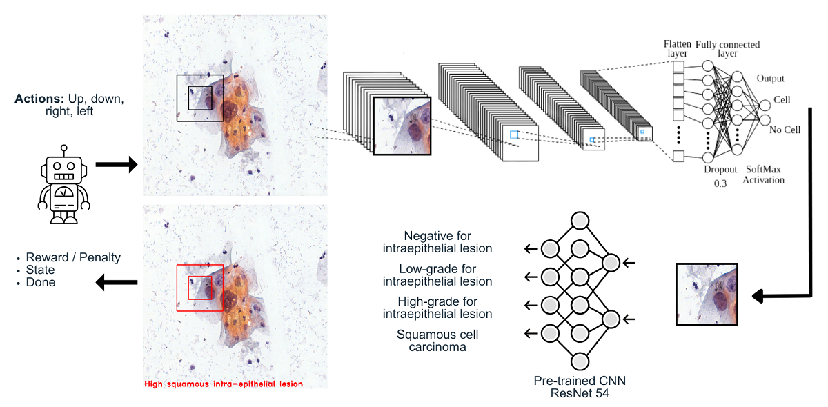
This paper focuses on overcoming barriers in the healthcare system, specifically the long waiting times that patients face when waiting for their test results. To address these issues and eliminate the long waiting times artificial intelligence (AI) techniques must be employed. This paper covers the implementation of a deep reinforcement learning (DRL) approach to identify the cells in digital Pap smear tests [8]. The proposed approach involves designing a DRL environment to train an agent using a robust algorithm such as Proximal Policy Optimization (PPO) [9]. The agent is a defined region of interest (ROI) that moves over a digital Pap smear test locating cells. The successful implementation of this technology could have a significant impact on reducing waiting times for patients and improving the efficiency of the healthcare system.
1. Materials and Methods
1.1. Data Acquisition
This paper used two datasets. The first dataset includes 2400 images of Pap tests that were collected from the Mendeley data repository. These samples were taken in 2019 from 460 patients at three Indian institutions: Babina Diagnostic Pvt. Ltd, Dr. B. Borooah Cancer Research Institute, and Gauhati Medical College and Hospital. To achieve higher-quality images with clearer backgrounds, liquid-based cytology was used instead of the conventional method. The images were captured using a Leica DM 750 microscope that was connected to a specialized high definition camera ICC50 HD, and the official computer software was utilized. The microscope’s magnification was set to 400x, resulting in high-definition JPG images with a resolution of 2048 x 1536 pixels [10].
Each image in the dataset was categorized by a pathologist into one of four categories, leading to the following classification, see Figure 1.
The second dataset was obtained from the bachelor’s thesis of Topapanta [11], who cropped the images from the first dataset to extract images with a size of 150 by 150 pixels that contains single cell and Pap smear background images. The dataset consists of 100 images that are classified into two categories: “Cells” and “No Cells”, see Figure 2 and Figure 3.
1.2. Agent Design
In reinforcement learning an agent refers to an intelligent entity that interacts with an environment in order to learn and optimize its decision-making process. It is capable of perceiving the state of the environment through observations and receives feedback in the form of rewards or penalties based on its actions [8]. This paper proposes an ROI that functions as an agent, see Figure 5. The ROI agent interacts with the environment by moving through the digital Pap smear performing some actions, see Table 1, and collecting the large amount of cells during an episode. The proposed ROI agent extends the capabilities of traditional digital Pap smear test analysis by introducing an intelligent entity that actively participates in the cell collection process. Through its interactions with the digital environment, the ROI agent aims to enhance the efficiency and effectiveness of the diagnostic procedure, ultimately leading to improved accuracy and reducing long waiting times for results.
2. Environment Design
The environment defines the rules, dynamics, and feedback mechanisms that govern the agent’s behavior and learning process. The environment consists of states, actions, rewards, and a transition model. States describe the current situation or configuration of the environment, while actions are the choices available to the agent to modify or interact with the environment. Additionally, the environment provides feedback to the agent in the form of rewards or penalties based on its actions. Rewards indicate the desirability or quality of the agent’s behavior, guiding it toward maximizing cumulative rewards over time. Providing the necessary stimuli and feedback for the agent to explore, learn, and improve its decision-making capabilities. The environment in this project follows the specifications outlined by GYM, which is a framework developed by OpenAI for creating and simulating interactive environments used in reinforcement learning (RL) tasks. It provides a standardized platform for designing RL experiments and allows researchers to define observation spaces, action spaces, rewards, episode termination conditions, and other environment-specific configurations. [12]. Finally, the entire digital Pap smear acts as the environment in which the agent can perform actions to navigate around the image and locate the cells presented in the sample, see Figure 4.
The observation space refers to a key feature in reinforcement learning environments. It represents the state or observation of the environment at any given time, providing information that the agent can perceive. The observation space defines the type and structure of the data that the agent receives as input. It could be in the form of raw sensory data, such as images, see Figure 5. By accessing the observation space, the agent can gather information about the environment’s features, conditions, or objects necessary for decision-making. It allows the agent to perceive and understand the current state of the environment, which enables it to select appropriate actions to achieve its objectives [13].
2.1. Reward Signal
The reward signal is a crucial component of the learning process. It represents the feedback provided to an agent based on its actions in an environment. The reward signal serves as a measure of the desirability or quality of the agent’s behavior, guiding it toward learning optimal or desirable policies. Also, it is typically a numerical scalar value that the agent receives from the environment after each action it takes. Furthermore, the reward signal can be explicitly provided by the environment, or it can be implicitly defined through a reward function, which maps states and actions to rewards. Finally, the reward function encapsulates the designer’s intentions and objectives, shaping the agent’s learning process. The reward signal can be written as R and it was defined as follows.
where n is the number of found cells.
2.2. Pseudocode
The environment has been developed using the object-oriented programming paradigm, allowing for efficient extraction of all its features through separate code segments. By adopting this approach, various aspects of the environment can be accessed and manipulated independently.
| Algorithm 1:Environment feature extraction |
|
2.3. Cell Recognition Model
The reward signal in the environment consists of predefined rewards and penalties that are determined based on whether the agent detects a cell or not. To ascertain that the agent is located over on a cell, a convolutional neural network (CNN) is employed. The CNN needs to provide a balance between small size and high accuracy, as computational efficiency is crucial during training. The neural network architecture begins with a convolutional layer that takes a pixel image as input and applies 10 filters sized . This is followed by a second convolutional layer with 32 filters of the same size. The final convolutional layer also employs 64 filters of size . The last convolutional layer is connected to a flatten layer, which is then followed by a dense layer with 16 neurons. In order to prevent overfitting, a dropout layer with a rate of 0.3 is implemented. Finally, a dense layer with 2 neurons determines whether the image corresponds to a cell or not, see Figure 6.
2.4. Cell Classifier Model
A pre-trained CNN was used in order to classify the cells. Residual Network (ResNet) is a deep convolutional neural network architecture introduced in 2015 by Kaiming He et al. in the paper “Deep Residual Learning for Image Recognition”, mention that the main idea behind ResNet is to address the issue of vanishing gradients in deep neural networks. Deep networks with many layers can suffer from vanishing gradients, where the magnitude of the gradients used to update the weights during training becomes very small, leading to slow convergence or even non-convergence. ResNet solves this problem by adding residual connections to the network, which allow the gradients to bypass one or more layers and flow more easily through the network [14]. A residual block in ResNet consists of several convolutional layers, with the output of each layer being added to the input of the next layer (the “residual connection”). This allows the network to learn residual functions, or the difference between the desired output and the input, instead of trying to learn the whole mapping from scratch [15] see Figure 7.
ResNet also introduced the concept of deep supervision, where multiple loss functions are used for different parts of the network to help improve convergence.
The ResNet architecture achieved state-of-the-art results on a number of computer vision benchmarks and has been widely used in many subsequent deep learning models and systems. It is also one of the most popular models for transfer learning, where a pre-trained ResNet model is fine-tuned for a new task [15]. Residual Network (ResNet) is capable of categorizing cells into the following categories mentioned in the first dataset see Figure 1.
In this work, ResNet-54 was used, where the number represents the total number of layers in the CNN. Nevertheless, it is necessary to emphasize that as the number of layers increases the computational cost too. This architecture was trained by using pre-default weights. This is useful for increasing the efficiency and precision of the model. As a consequence, it helps the network to converge faster, having an accurate model in less time. ResNet-54 is trained with a set of data from ImageNet that can be used to initialize the network before being trained with different data, see Fig Figure 1. This network already has knowledge about how to recognize and extract image features. To avoid over-fitting a dropout is added in the last layer of ResNet-54. The dropout is a hyper-parameter, and regularization technique where the main idea is forcing some neurons to not activate during the training [16]. For this architecture, the dropout was added in the last convolutional layer with a rate of 0.3.
2.5. Training Process
In reinforcement learning, there are many different algorithms that may be used to train agents. Choosing the right algorithm is essential in order to converge to a good behavior. The agent uses PPO for training since it has been shown to be reliable and effective in many applications [9,17,18]. PPO ensures that the changes made to the policy distribution remain within a specified range. This constraint is vital for maintaining stability during the learning process, as it prevents extreme policy updates that may result in divergent behavior or sub-optimal policies. Furthermore, PPO incorporates a clipping mechanism within the surrogate objective function, limiting the policy update to a certain threshold. This clipping helps to stabilize the learning process by preventing overly large policy updates, which can introduce instability and hinder convergence. The ROI uses this on-policy algorithm to train and learn, see Algorithm 2, how to move in the environment and what features are important to solve the task.
| Algorithm 2:PPO Clip |
|
2.6. Experiments
A total of eight agents will be trained using different reward signals, see Table 2. The PPO algorithm hyperparameters are tuned in order to test the best configuration. The first four agents (A-D) have a n_step value set to 512. Conversely, the remaining four agents (E-H) employ identical hyperparameters, but with a n_step value of 1024, see Table 3.
Finally, the selection of agents for further consideration relies on their performance throughout the training process. To facilitate this selection, a multi-stage approach is implemented, involving three distinct stages for rejecting agents and not well-defined reward signals. This process aims to identify the most promising agents from each stage and subject them to retraining in subsequent stages, see Figure 8.
3. Results and Discussion
3.1. First Stage
In the initial phase, we observed the initial training progress of the agents, see Figure 9 and Figure 10. It became apparent that the two agents failed to construct a viable policy. This outcome arose due to the inadequately defined reward signal, which imposed a significant penalty on the agents for cell searching. On the other hand, the remaining six agents exhibited diverse mean rewards over the course of their training. Notably, agents C, E, and F outperformed the others by executing more effective actions and detecting a greater number of cells. Consequently, these agents achieved higher mean rewards throughout the three-million-time training period and demonstrated stability in their performance values.
The variations in mean rewards can be attributed to the random selection of environments or digital Pap smears from the initial dataset. Each environment contained a different number of cells, which introduced variability into the agents’ experiences. Furthermore, the initial peak observed in all the agents’ performance can be attributed to the fact that the initial policies were not yet well-trained. These early policies often generated a large number of random actions, which resulted in the agents covering a larger area of the environment. However, since these actions were chosen randomly without any prior experience or knowledge, the agents did not gain meaningful insights or improve their performance significantly during this peak.
3.2. Second Stage
In this stage, agents C, E, and F were selected based on their superior performance, as they consistently achieved higher mean rewards compared to the other agents. These selected agents underwent an additional two million time steps of retraining, leading to diverse outcomes, as depicted in Figure 11. Agent E emerged as the standout learner during this stage, exhibiting positive mean rewards and surpassing the performance of the other agents. However, it is worth mentioning that in one particular environment, agent E obtained lower values compared to the other environments. After that lowest value, the agent began to recover its policy and exhibit improved results. On the other hand, agents C and F consistently obtained negative mean rewards in the majority of environments, leading to their exclusion from the final stage. The negative mean rewards obtained by agents C and F indicated a lack of effective policy and performance in various environments. These agents were therefore considered unsuitable to advance to the final training level.
3.3. Third Stage
In this stage, agent E underwent parallel retraining for 6 million additional time steps, carried out four times. Surprisingly, as depicted in Figure 5.6, despite employing identical hyperparameters and a shared pre-trained model, the learning process exhibited variability. This variation can be attributed to the use of a stochastic algorithm, which generates a policy based on action probabilities rather than deterministic choices. The stochastic nature of the algorithm introduces randomness into the learning process, resulting in divergent training trajectories. As a result, each retrained agent may exhibit unique patterns of improvement and performance. From the four retrained agents, it is possible to select one agent that achieves superior results compared to the others. This selection is based on the agent’s ability to optimize its policy and achieve higher performance scores. This highlights the importance of evaluating and identifying the most successful agent among multiple retraining iterations.
3.3.1. Behavior Testing
Now, it is interesting to see the agents’ movement patterns within the environment. To visualize their trajectories and action frequencies, a heatmap technique was employed. Figure 13 showcases this representation, highlighting the agents’ positions and the frequency of actions taken in each location. The heatmap provides valuable insights into how the agents navigate and interact with the environment. By observing the intensity of color in different areas, we can identify regions where the agents spend more time or take repetitive actions. This visualization aids in understanding the agents’ exploration patterns and potential areas of focus.
To assess the behavior of the agents, three distinct environments were chosen for policy testing. Each environment featured a different quantity of cells distributed throughout various sections of the test area, see Figure 14. By defining these diverse environments, we aimed to evaluate how the agents are adapting and performing under different conditions. The varying distribution of cells provided a challenge for the agents to locate and identify them effectively. This approach allowed us to analyze the agents’ performance across different scenarios, gaining insights into their capabilities and strategies in different parts of the test.
In the first environment, see Figure 15, It is interesting to observe that agent E1 displayed no behavior in the first environment, despite achieving higher mean rewards in training compared to the other agents in multiple environments. Analyzing the heatmap plots of agents E2 and E4, we can observe that these agents actively search for cells but eventually become trapped in a repetitive loop of actions. On the other hand, the heatmap plot of agent E3 shows a notable performance, as it covers a larger area compared to the other agents and successfully detects nearly all the cells present in the sample. Additionally, agent E3 exhibits a maximum of 20 passes through the same position, indicating efficient exploration and reduced redundancy in actions. Overall, these observations suggest that agent E3 demonstrates superior performance in terms of coverage, cell detection, and avoidance of repetitive behavior in the given environment.
In the second environment, see Figure 16, we observe that agent E1 remains trapped in the initial position throughout the entire episode without taking any actions. This indicates a lack of exploration or an inability to navigate effectively in this particular environment. Conversely, agents E2 and E4 exhibit more active behavior and successfully identify a significant number of cell positions. However, they eventually fall into repetitive action patterns, suggesting a limitation in their ability to adapt and explore further. Additionally, agent E3 once again stands out with impressive results. It achieves a high level of visual coverage, capturing almost all the cells, while demonstrating a maximum of 20 repetitions of passing through the same position. Furthermore, agent E3 covers a larger area compared to the other agents, indicating a more comprehensive exploration. In sum, these findings highlight the superior performance of agent E3 in terms of cell detection, reduced repetitive actions, and broader area coverage, making it the most promising agent in the second environment.
In the third environment, see Figure 17, we observe that agent E1 actively performs actions and successfully collects a significant number of cells compared to the other environments. This behavior can be attributed to the fact that more training steps are required for agent E1 to overcome the difficulty of getting stuck in the starting position. After visual analysis of the other agents, we can infer that they exhibit a searching behavior, trying to maximize the number of found cells in the environment. Each agent has unique search patterns as they explore. However, a common issue arises: the agents tend to fall into repetitive action loops. It is evident that the agents would benefit from further retraining to prevent this repetitive behavior and optimize their search strategies. However, despite this limitation, the agents still display a strong inclination towards exploring and gathering cells.
3.4. Cell Classifier Model
Training a model using a ResNet50 architecture with pre-trained weights offers numerous advantages over training from scratch. Pre-trained weights allow the model to take advantage of the knowledge acquired from a large dataset like ImageNet, which contains millions of labeled images. These pre-trained weights encapsulate general image features, including edges, textures, and object parts, which prove advantageous for transfer learning. This initialization provides the model with a robust starting point, enabling faster convergence and superior performance compared to training from zero, see Figure 18 and Figure 19.
After training the model for classifying cervix cells in digital Pap smears, the results showed a training loss and accuracy of 26.40% and 89.89%, respectively. When the model was tested on new data, it achieved a validation loss and accuracy of 21.30% and 91.25%, respectively. Furthermore, Table 4 highlights the excellent classification performance of the model across different cervix cell types. It achieves an accuracy of 89.88% in identifying HSIL, demonstrating its capability to accurately detect this severe abnormality. Additionally, the model exhibits a high accuracy of 92.27% for LSIL, effectively distinguishing this less severe abnormality. Notably, It shows excellent performance in classifying NILM cases, achieving an accuracy of 98.51%. Moreover, the model achieves a respectable accuracy of 83.40% for SCC, crucial for the early detection and treatment of this malignant condition.
By integrating a cell classifier model into the environment and leveraging the intelligence of trained agents, we can create a highly advanced system for detecting and classifying located cells. In the final environment, the trained agents operate autonomously, utilizing cell recognition to scan their surroundings and identify cells in real time. Once a cell is detected, the agents employ the cell classifier model to classify it according to predefined categories, see Figure 20.
4. Conclusion
In conclusion, the trained agents have demonstrated exceptional learning capabilities, and they have successfully developed a searching behavior that allows them to efficiently locate cells within digital Pap smears. These results indicate the effectiveness of the deep reinforcement learning approach in navigating complex visual patterns and identifying cells of interest.
Additionally, a CNN model using ResNet-54 architecture was trained to classify the detected cells into four distinct categories including negative for intraepithelial lesion or malignancy, low-grade intraepithelial lesions, high-grade intraepithelial lesions, and squamous cell carcinoma. This classification capability adds another layer of sophistication to the proposed system, enabling accurate identification and categorization of cells based on their shape and structure.
The successful training of both the agents and the CNN model shows the potential of this research to revolutionize the field of cervical cancer screening. By combining the searching behavior of the agents with the classification capabilities of the CNN model, an integrated and highly efficient system for automated analysis of Papanicolaou can be realized.
These results have important implications for clinical practice, as they open the door for the development of an automatic Papanicolaou analyzing machine that can analyze samples without human intervention. The utilization of deep reinforcement learning and CNN-based classification techniques has the potential to solve the lack of pathologists, particularly in low-middle incoming countries, and improve the accuracy and availability of cervical cancer screening services.
In conclusion, our research has successfully trained four agents over 11 million time steps, resulting in the development of a searching behavior for locating cells in digital Pap smear images. Furthermore, our CNN model, utilizing the ResNet-54 architecture, accurately classifies the detected cells into four categories. These achievements demonstrate the great capabilities of deep reinforcement learning and CNN-based classification techniques in advancing the field of cervical cancer screening. The proposed automated system could improve the efficiency, accessibility, and accuracy of Papanicolaou analysis, ultimately contributing to the global efforts of eliminating cervical cancer and improving women’s healthcare worldwide.
Author Contributions
Conceptualization, Oscar Chang; Formal analysis, Carlos Macancela; Resources, Oscar Chang; Software, Carlos Macancela and Manuel Eugenio Morocho Cayamcela; Supervision, Manuel Eugenio Morocho Cayamcela and Oscar Chang; Validation, Manuel Eugenio Morocho Cayamcela and Oscar Chang; Writing – original draft, Carlos Macancela; Writing – review & editing, Manuel Eugenio Morocho Cayamcela and Oscar Chang
Data Availability Statement
We encourage all authors of articles published in MDPI journals to share their research data. In this section, please provide details regarding where data supporting reported results can be found, including links to publicly archived datasets analyzed or generated during the study. Where no new data were created, or where data is unavailable due to privacy or ethical restrictions, a statement is still required. Suggested Data Availability Statements are available in section “MDPI Research Data Policies” at https://www.mdpi.com/ethics.
Acknowledgments
In this section you can acknowledge any support given which is not covered by the author contribution or funding sections. This may include administrative and technical support, or donations in kind (e.g., materials used for experiments).
Conflicts of Interest
The authors declare no conflict of interest.
References
- Cohen, P.A.; Jhingran, A.; Oaknin, A.; Denny, L. Cervical cancer. The Lancet 2019, 393, 169–182. [Google Scholar] [CrossRef] [PubMed]
- Hasenleithner, S.O.; Speicher, M.R. How to detect cancer early using cell-free DNA. Cancer Cell 2022, 40, 1464–1466. [Google Scholar] [CrossRef]
- Nuche-Berenguer, B.; Sakellariou, D. Socioeconomic determinants of cancer screening utilisation in Latin America: A systematic review. PLOS ONE 2019, 14, e0225667. [Google Scholar] [CrossRef] [PubMed]
- Davies-Oliveira, J.; Smith, M.; Grover, S.; Canfell, K.; Crosbie, E. Eliminating Cervical Cancer: Progress and Challenges for High-income Countries. Clinical Oncology 2021, 33, 550–559. [Google Scholar] [CrossRef] [PubMed]
- Organization, W.H. Cervical cancer ecuador 2021 country profile, 2021.
- Liebermann, E.J.; VanDevanter, N.; Hammer, M.J.; Fu, M.R. Social and Cultural Barriers to Women’s Participation in Pap Smear Screening Programs in Low- and Middle-Income Latin American and Caribbean Countries: An Integrative Review. Journal of Transcultural Nursing 2018, 29, 591–602. [Google Scholar] [CrossRef] [PubMed]
- Strasser-Weippl, K.; Chavarri-Guerra, Y.; Villarreal-Garza, C.; Bychkovsky, B.L.; Debiasi, M.; Liedke, P.E.R.; de Celis, E.S.P.; Dizon, D.; Cazap, E.; de Lima Lopes, G.; et al. Progress and remaining challenges for cancer control in Latin America and the Caribbean. The Lancet Oncology 2015, 16, 1405–1438. [Google Scholar] [CrossRef] [PubMed]
- Sutton, R.S.; Barto, A.G. Reinforcement Learning: An Introduction, second ed.; The MIT Press: Cambridge, 2018. [Google Scholar]
- Schulman, J.; Wolski, F.; Dhariwal, P.; Radford, A.; Klimov, O. 2017; arXiv:1707.06347]. [CrossRef]
- Hussain, E.; Mahanta, L.B.; Borah, H.; Das, C.R. Liquid based-cytology Pap smear dataset for automated multi-class diagnosis of pre-cancerous and cervical cancer lesions. Data in Brief 2020, 30, 105589. [Google Scholar] [CrossRef] [PubMed]
- Chang, O.G.; Toapanta, B.O. Automatic high-resolution ananlysis of pap test cells, 2021.
- Brockman, G.; Cheung, V.; Pettersson, L.; Schneider, J.; Schulman, J.; Tang, J.; Zaremba, W. OpenAI Gym. In Proceedings of the International Conference on Learning Representations; 2016. [Google Scholar]
- Plappert, M.; Houthooft, R.; Dhariwal, P.; Sidor, S.; Chen, R.Y.; Asfour, T.; Abbeel, P.; Andrychowicz, M. Multi-Goal Reinforcement Learning: Challenging Robotics Environments and Request for Research. In Proceedings of the Conference on Robot Learning; 2018. [Google Scholar]
- Targ, S.; Almeida, D.; Lyman, K. Resnet in resnet: Generalizing residual architectures, 2016. [CrossRef]
- He, F.; Liu, T.; Tao, D. Why resnet works? residuals generalize. IEEE transactions on neural networks and learning systems 2020, 31, 5349–5362. [Google Scholar] [CrossRef] [PubMed]
- Chen, L.; Gautier, P.; Aydore, S. DropCluster: A structured dropout for convolutional networks, 2020. [CrossRef]
- OpenAI., *!!! REPLACE !!!*; :., *!!! REPLACE !!!*; Berner, C.; Brockman, G.; Chan, B.; Cheung, V.; Debiak, P.; Dennison, C.; Farhi, D.; Fischer, Q. OpenAI.; :.; Berner, C.; Brockman, G.; Chan, B.; Cheung, V.; Debiak, P.; Dennison, C.; Farhi, D.; Fischer, Q.; et al. Dota 2 with Large Scale Deep Reinforcement Learning, 2019. [CrossRef]
- OpenAI., *!!! REPLACE !!!*; Akkaya, I.; Andrychowicz, M.; Chociej, M.; Litwin, M.; McGrew, B.; Petron, A.; Paino, A.; Plappert, M.; Powell, G. OpenAI.; Akkaya, I.; Andrychowicz, M.; Chociej, M.; Litwin, M.; McGrew, B.; Petron, A.; Paino, A.; Plappert, M.; Powell, G.; et al. 2019; arXiv:1910.07113]. [Google Scholar] [CrossRef]
Figure 1.
Pap smear samples: (a) Negative for intraepithelial lesion or malignancy (NILM) (b) Low-grade intraepithelial lesions (LSIL) (c) High-grade intraepithelial lesions (HSIL) and (d) Squamous Cell Carcinoma (SCC).
Figure 1.
Pap smear samples: (a) Negative for intraepithelial lesion or malignancy (NILM) (b) Low-grade intraepithelial lesions (LSIL) (c) High-grade intraepithelial lesions (HSIL) and (d) Squamous Cell Carcinoma (SCC).
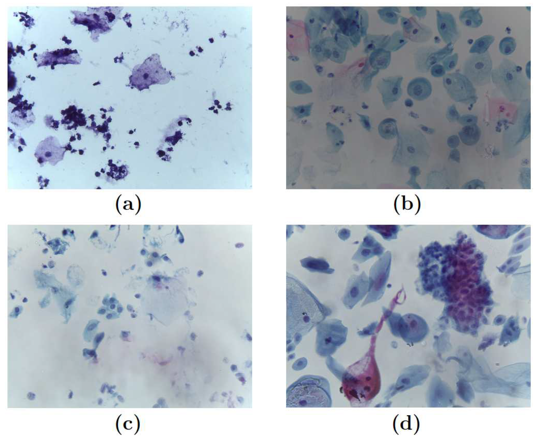
Figure 2.
Examples of extracted “Cells”.
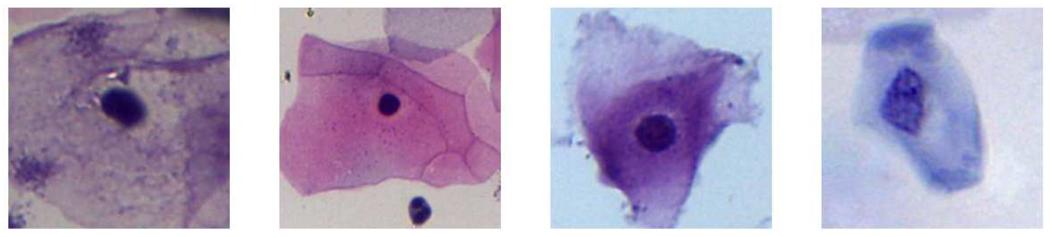
Figure 3.
Examples of extracted “No cells”.
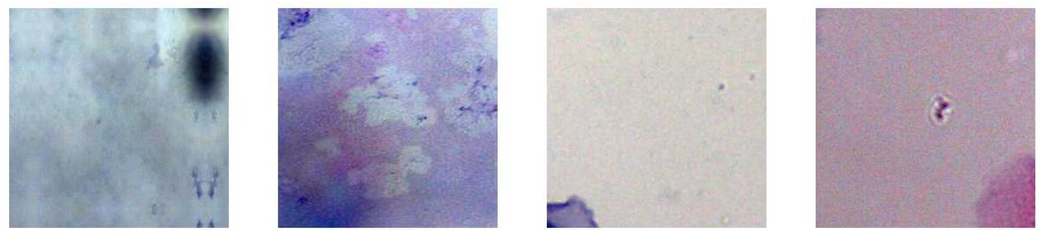
Figure 4.
Graphical representation of two environments. A) It is the environment where the agent searches for cells, and the captured image by the ROI is displayed in the right window. B) displays the cells that have been detected.
Figure 4.
Graphical representation of two environments. A) It is the environment where the agent searches for cells, and the captured image by the ROI is displayed in the right window. B) displays the cells that have been detected.

Figure 5.
The figure illustrates a stack of frames, visually representing the environment in which an agent interacts. The agent is characterized by two black squares and the motion it exhibits within the frames.
Figure 5.
The figure illustrates a stack of frames, visually representing the environment in which an agent interacts. The agent is characterized by two black squares and the motion it exhibits within the frames.
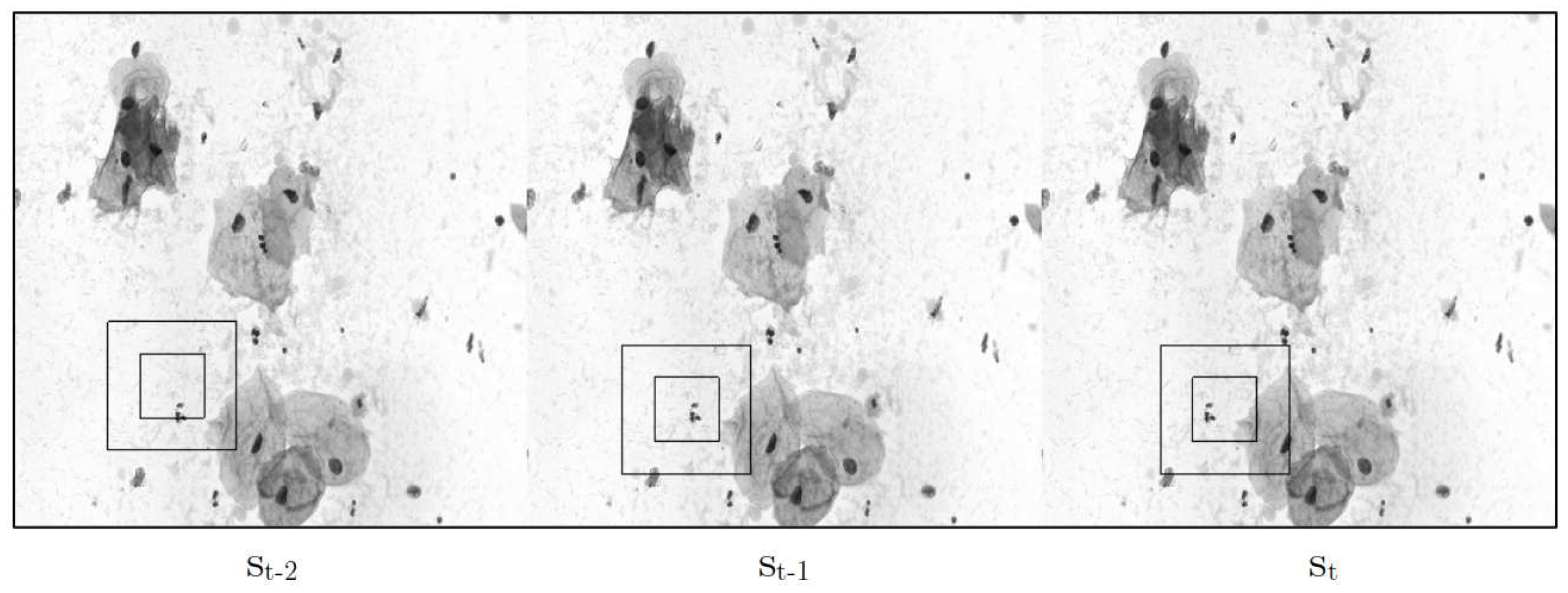
Figure 6.
A visual depiction of how data moves through the CNN.
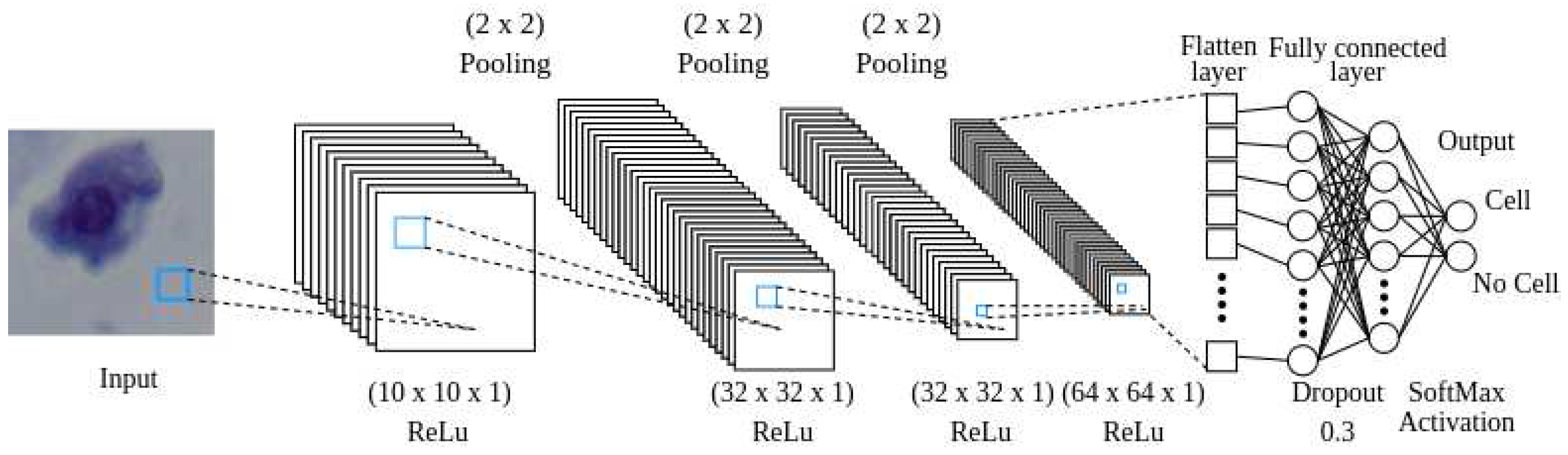
Figure 7.
Residual block architecture of ResNet model
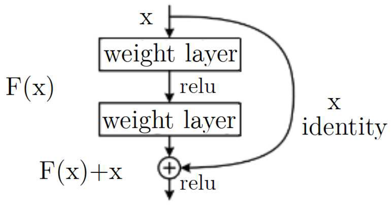
Figure 8.
Graphic representation of the stages during the training process.
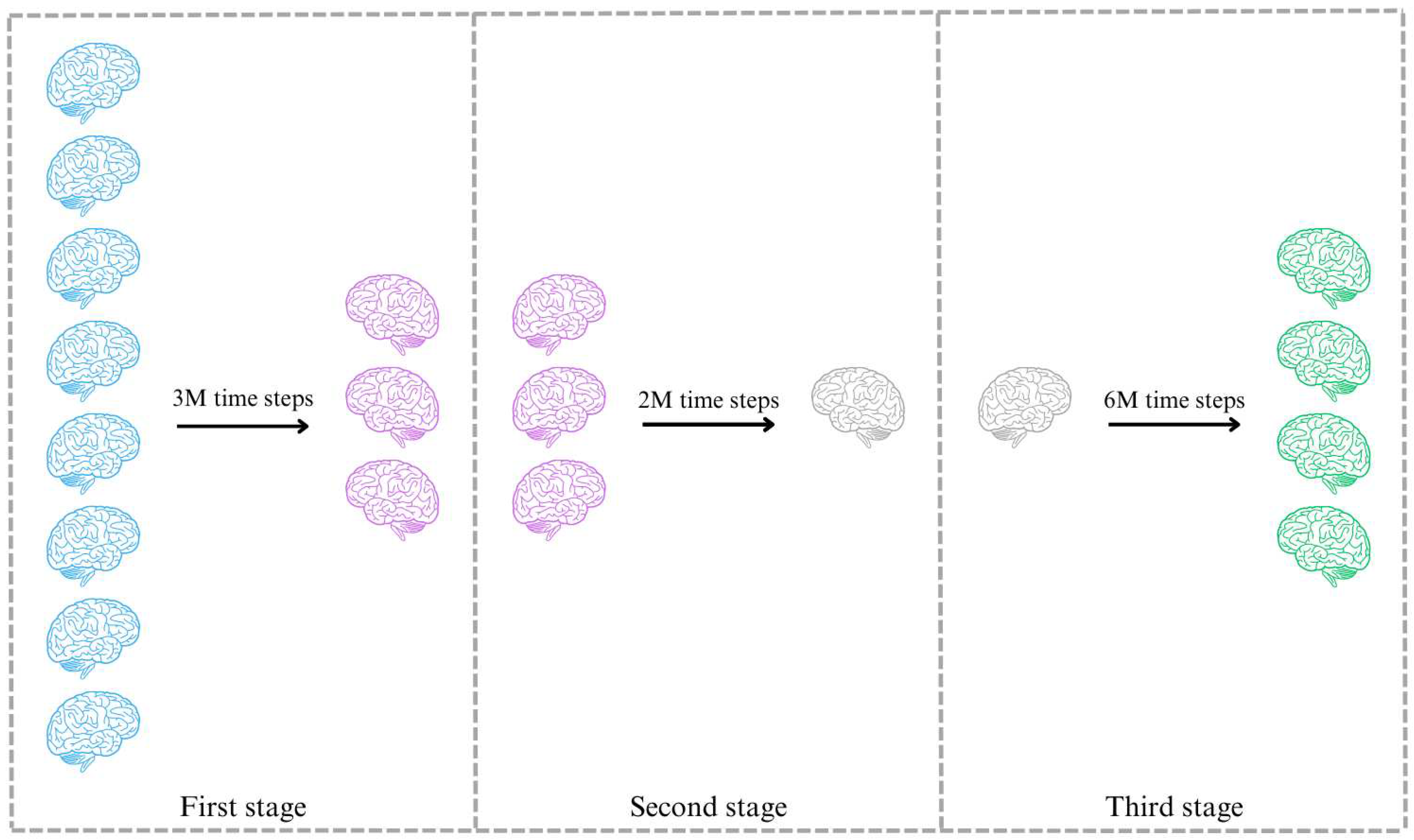
Figure 9.
The left plot shows all the first set of agents’ mean rewards, permitting the ability to visually compare their training process. The right plot shows only three agents, agent D was not considered because it has the lowest values.
Figure 9.
The left plot shows all the first set of agents’ mean rewards, permitting the ability to visually compare their training process. The right plot shows only three agents, agent D was not considered because it has the lowest values.
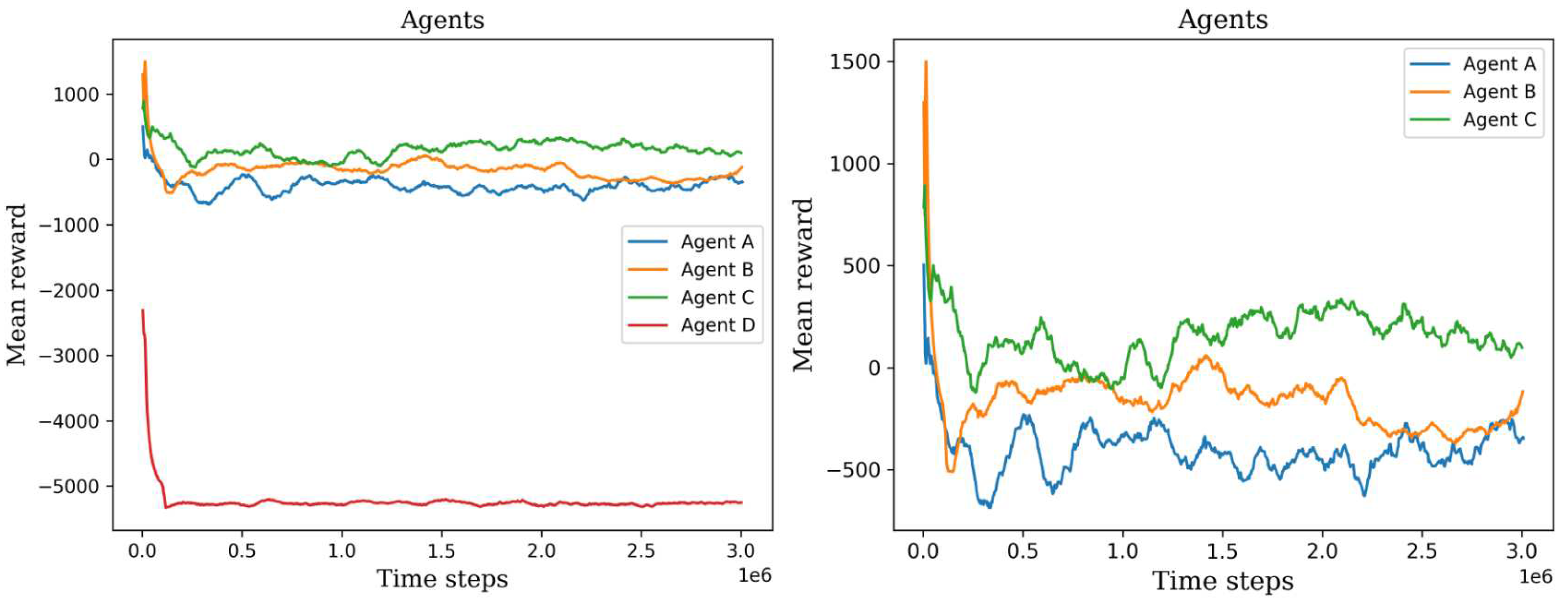
Figure 10.
The left plot shows all the second set of agents’ scores, permitting the ability to visually compare their training process. The right plot shows only three agents, agent H was not considered because it has the lowest values.
Figure 10.
The left plot shows all the second set of agents’ scores, permitting the ability to visually compare their training process. The right plot shows only three agents, agent H was not considered because it has the lowest values.
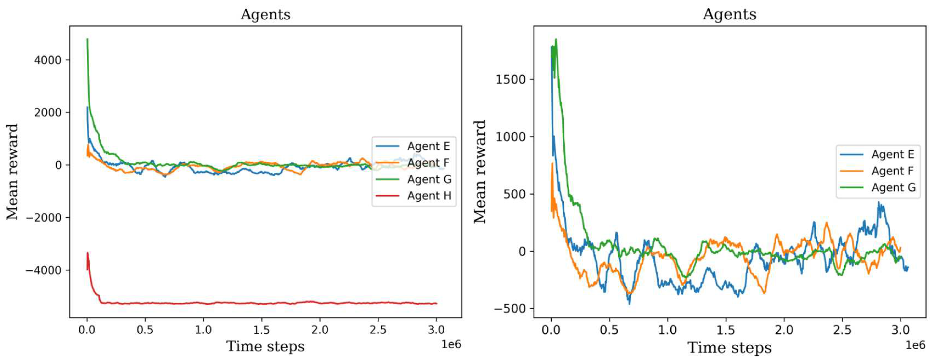
Figure 11.
The graph shows the retraining results of the agents C, E, and F.
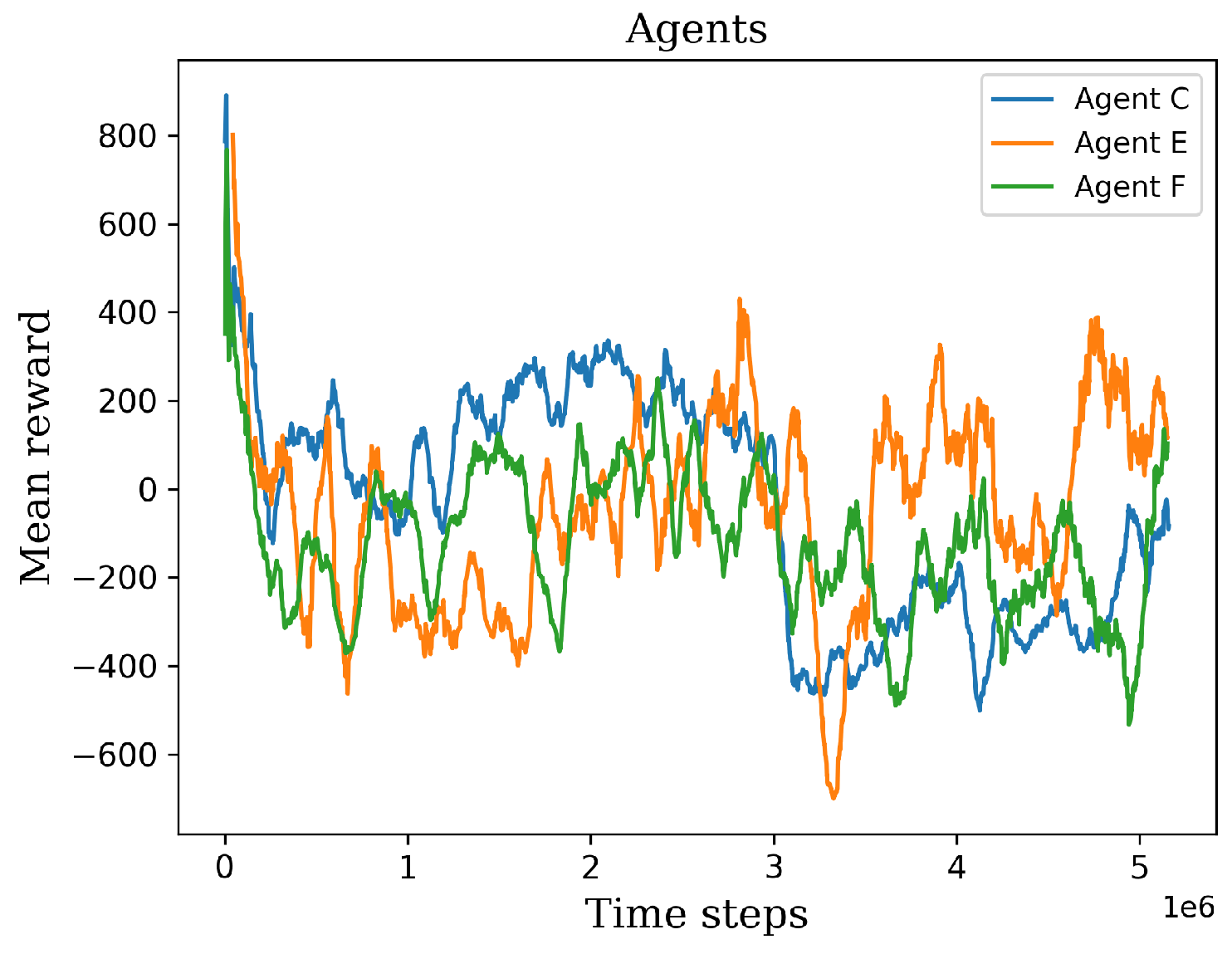
Figure 12.
The graph shows the retraining results of the four extensively trained agents.
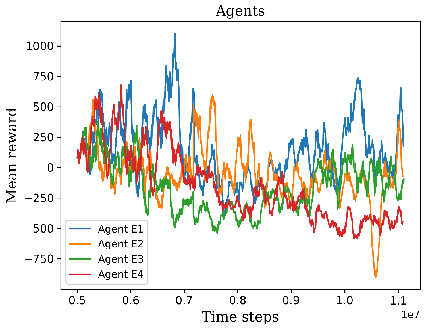
Figure 13.
The figure illustrates the behavior of an untrained agent. Red dots represent discovered cells, while the blue bar indicates repetitive visits to the same position.
Figure 13.
The figure illustrates the behavior of an untrained agent. Red dots represent discovered cells, while the blue bar indicates repetitive visits to the same position.
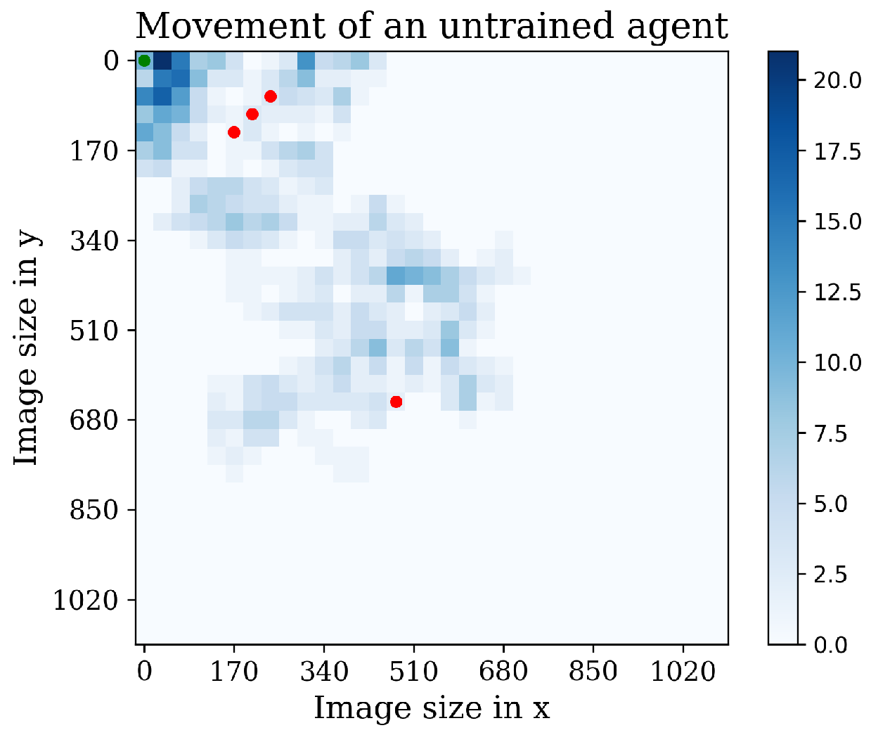
Figure 14.
The figure shows three distinct environments utilized for testing the agents during the second and third stages of experiments.
Figure 14.
The figure shows three distinct environments utilized for testing the agents during the second and third stages of experiments.
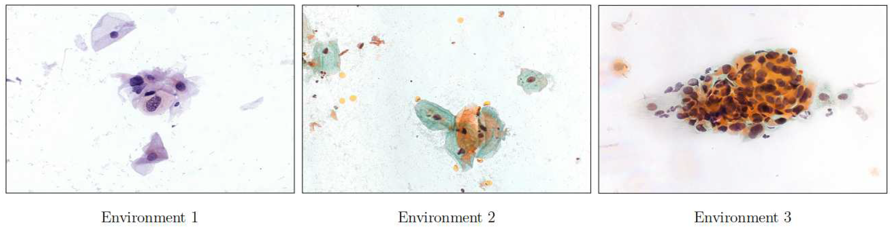
Figure 15.
Tracking results of the agents E1, E2, E3, E4 from the last stage in the first environment.
Figure 15.
Tracking results of the agents E1, E2, E3, E4 from the last stage in the first environment.
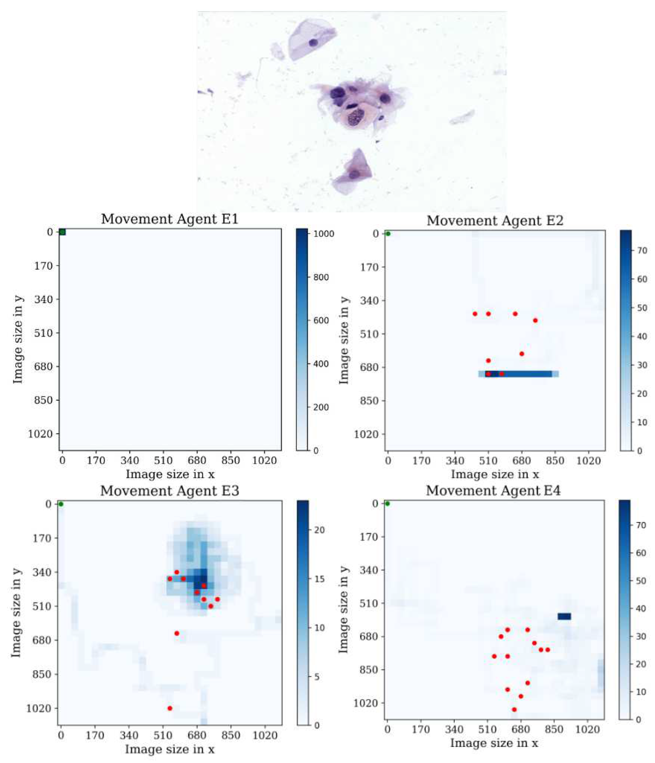
Figure 16.
Tracking results of the agents E1, E2, E3, E4 from the last stage in the second environment.
Figure 16.
Tracking results of the agents E1, E2, E3, E4 from the last stage in the second environment.
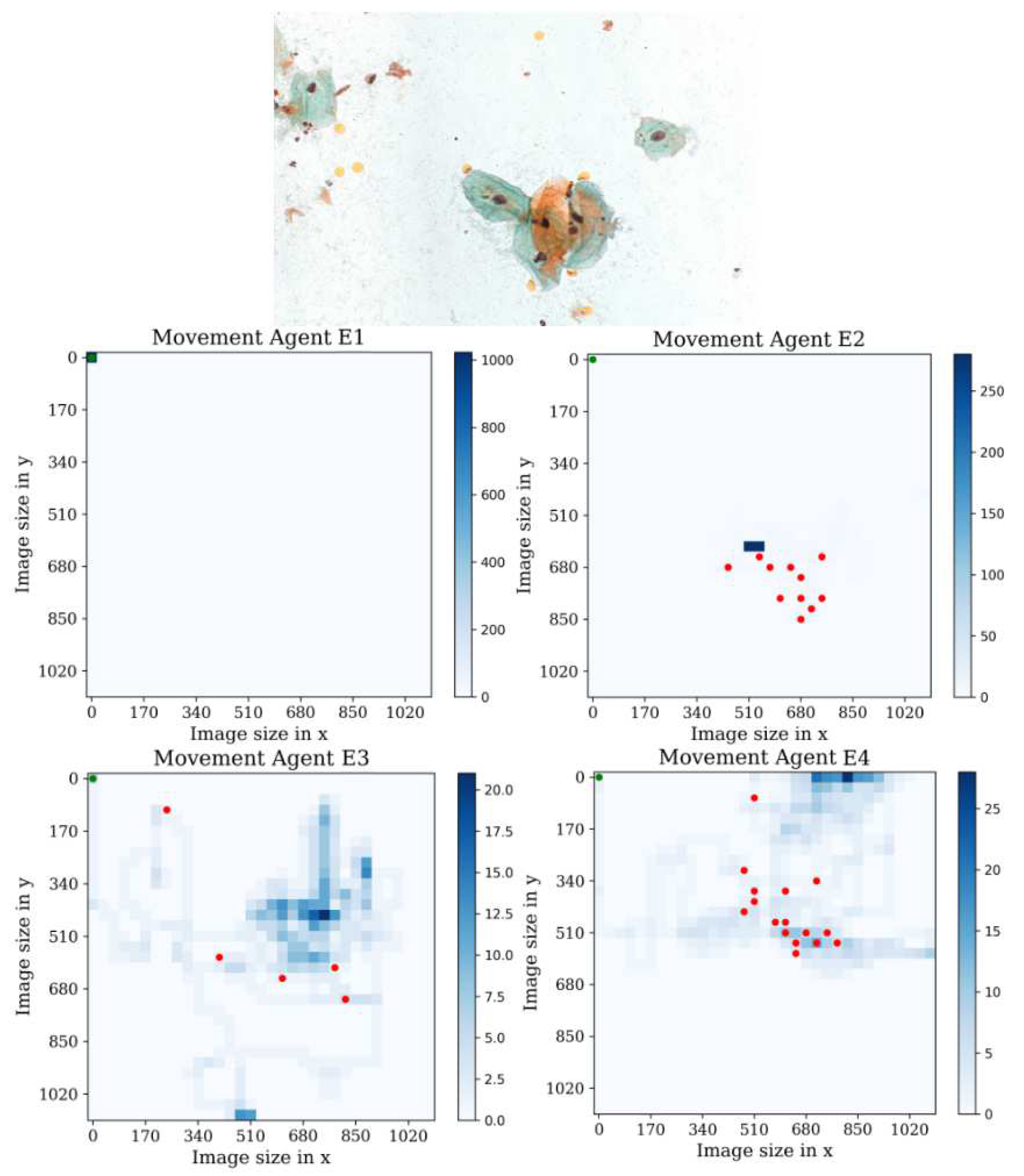
Figure 17.
Tracking results of the agents E1, E2, E3, E4 from the last stage in the third environment.
Figure 17.
Tracking results of the agents E1, E2, E3, E4 from the last stage in the third environment.
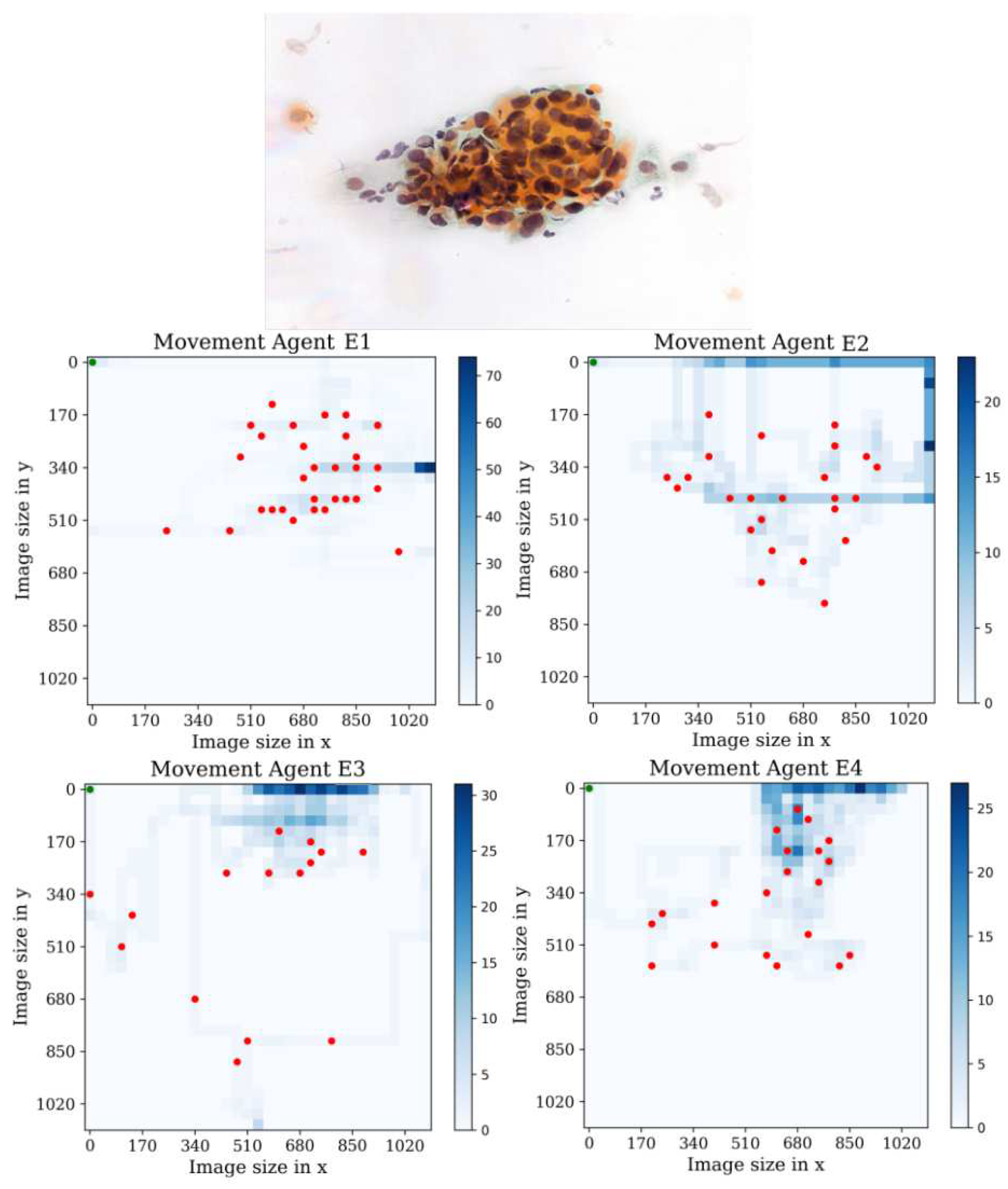
Figure 18.
ResNet-54 behavior in training and validation accuracy during 100 epochs.
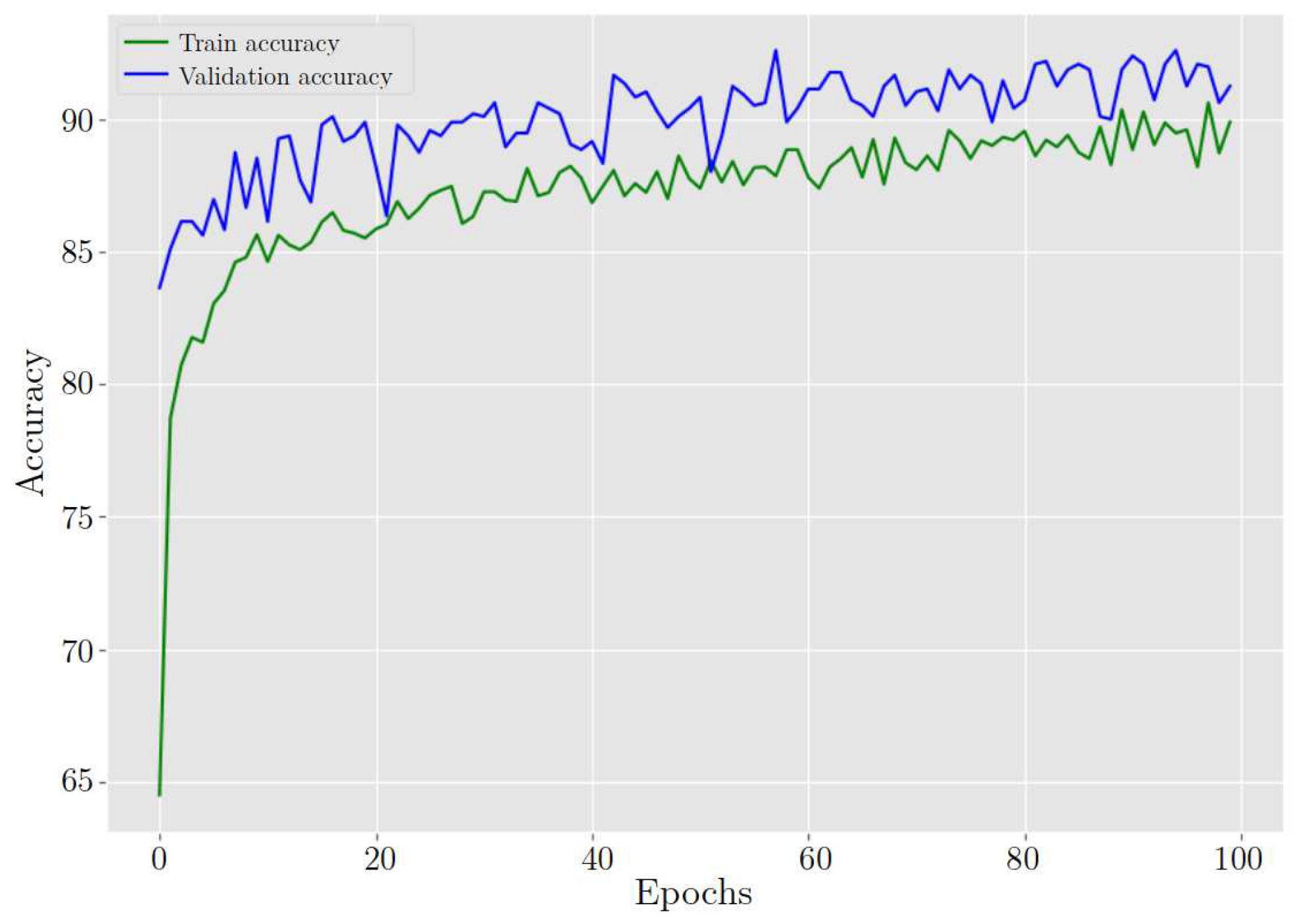
Figure 19.
ResNet-54 behavior in training and validation loss during 100 epochs.
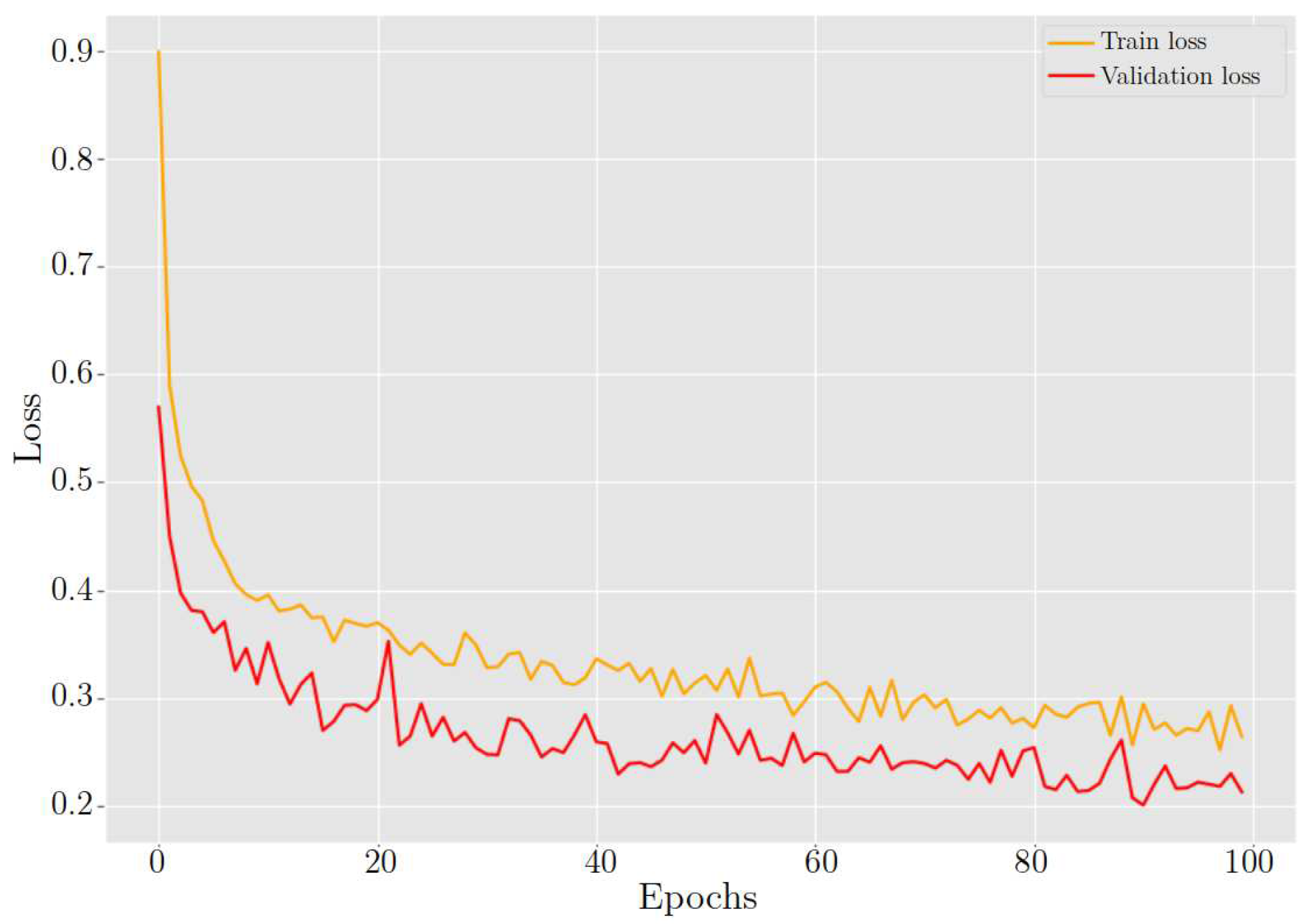
Figure 20.
The figure demonstrates three instances in which the agent successfully detects cells and accurately classifies them. The agent detected LSHL, HSIL, and SCC cells.
Figure 20.
The figure demonstrates three instances in which the agent successfully detects cells and accurately classifies them. The agent detected LSHL, HSIL, and SCC cells.
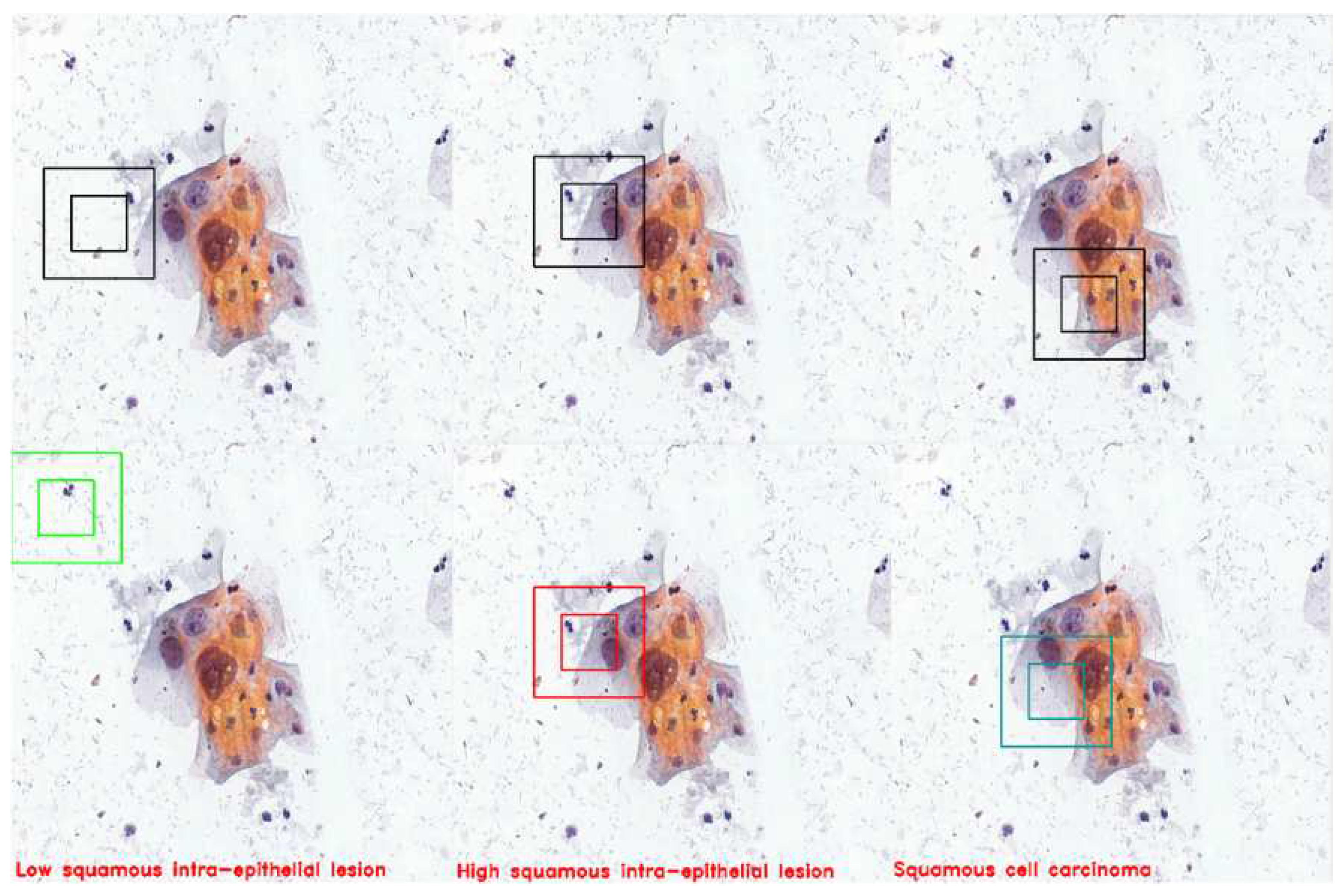

Table 1.
Agent’s actions.
| Actions # | Action |
|---|---|
| 1 | Right |
| 2 | Left |
| 3 | Up |
| 4 | Down |
Table 2.
Brief description of the agents.
| Agents | Description |
|---|---|
| A, E | Using the reward signal without changes. |
| B, F | No penalty for detecting the same cell multiple times |
| C, G | No penalty while searching for a cell |
| D, H | High penalty while searching for a cell, |
Table 3.
The hyperparameters included in the PPO Stable Baselines 3 implementation, with descriptions and values. The symbol following a hyperparameter name refers to the coefficient.
Table 3.
The hyperparameters included in the PPO Stable Baselines 3 implementation, with descriptions and values. The symbol following a hyperparameter name refers to the coefficient.
| Hyperparameters | Values | Description |
|---|---|---|
| learning_rate | Progress remaining, which ranges from 1 to 0. | |
| n_steps | 512;1024 | Steps per parameters update. |
| batch_size | 128 | Images processed by the network at once |
| n_epochs | 10 | Updates for the policy using the same trajectory |
| gamma | Discount factor | |
| gae_lambda | Bias vs. variance trade-off | |
| clip_range | Range of clipping | |
| vf_coef | Value function coefficient | |
| ent_coef | Entropy coefficient | |
| max_grad_norm | Clips gradient if it gets too large |
Table 4.
Validation accuracy of categories
| Categories | ResNet-54 |
|---|---|
| High-grade squamous intraepithelial lesion | 89.88% |
| Low-grade squamous intraepithelial lesion | 92.27% |
| Negative for intraepithelial lesion | 98.51% |
| Squamous cell carcinoma | 83.40% |
Disclaimer/Publisher’s Note: The statements, opinions and data contained in all publications are solely those of the individual author(s) and contributor(s) and not of MDPI and/or the editor(s). MDPI and/or the editor(s) disclaim responsibility for any injury to people or property resulting from any ideas, methods, instructions or products referred to in the content. |
© 2023 by the authors. Licensee MDPI, Basel, Switzerland. This article is an open access article distributed under the terms and conditions of the Creative Commons Attribution (CC BY) license (https://creativecommons.org/licenses/by/4.0/).
Copyright: This open access article is published under a Creative Commons CC BY 4.0 license, which permit the free download, distribution, and reuse, provided that the author and preprint are cited in any reuse.


