Submitted:
19 October 2023
Posted:
20 October 2023
You are already at the latest version
Abstract
In recent years, the economies of many countries of the world are in a situation of intense shock processes. The current situation urgently needs to change the economic paradigm in the near future, which objectively requires the development of new conceptual models. The purpose of the paper is to develop the basic theoretical provisions of a new macroeconomics based on impulse and jump processes. Research problems are the following: 1) to describe the main types of impulse and jump functions with examples from economic theory and practice; 2) to perform an analytical representation of impulse and jump functions; 3) to select macroeconomic characteristics for the analysis of rapidly changing processes in the economy; 4) to create models and mechanisms for predicting impulsive and abrupt changes in macroeconomics. The approaches to the development of macroeconomic theory and its methods proposed in the article are not associated with the use of evolutionary continuous functions, for example, power functions, which is typical for many canonical macroeconomic models. These approaches do not include management decisions to achieve optimal values of given target functions, which is typical for recursive macroeconomic models of dynamic programming. This article is about formulating the foundations of macroeconomic theory and its methods, which, with some degree of accuracy, could give a forecast about the impending possibility of abrupt changes (impulse, shock, jump, stepwise and others) in the macroeconomic situation. The research methodology is statistical analysis, special methods for studying impulse and jump processes developed by the author. As a result of the study, the main provisions of the macroeconomic theory based on rapid impulse and spasmodic changes were formulated, approaches were outlined for constructing the tools of this theory, problems and tasks for further research were identified.
Keywords:
macroeconomics
; theoretical foundations
; impulse and jump characteristics
MSC: 37N40
1. Introduction
There are a lot of problems in this area. But two main questions are the following: “Why are some
countries rich and others poor?”, and “Why does the economy in some countries
grow fast and in others slowly?” [1]. To answer these questions, we need to analyze data
relating to the economic performance of various countries.
Currently, there
are different models of economic growth. Let's look at the most famous of them.
The foundations of
modern growth theory were laid by Nobel Prize winner R. Solow, having developed
the neoclassical theory of economic growth [2], in which the
main role was played by the accumulation of physical capital. Solow also showed
for the first time that the key factor of economic growth is technical
progress, which he set exogenously [3]. The main focus of the Solow model, along with
traditional issues of capital accumulation, is on the relationship between the
two main factors of production - labor and capital, as well as their
relationship with the exogenous source of changes in productivity - technical
progress. Solow's growth theory, like all classical growth theories,
is based on the law of diminishing returns of factors, which is the main
condition for achieving an equilibrium state and sustainable development.
According to this law, under constant technical conditions, a consistent
increase in any of the production factors by an additional unit, with the
others remaining unchanged, leads to a decreasing increase in production. This
occurs under conditions of perfect competition. The production function in the
economic growth model is the Cobb-Douglas function, which includes a power
function, the basis of which is physical capital, and the exponent varies from
zero to one. The mathematical basis of Solow's economic growth model is the
first-order Bernoulli differential equation.
From the point of view of this article, the
disadvantage of the Solow model is that it is based on continuous functions and
does not take into account impulse, shock, step, spasmodic and other types of
rapidly changing processes characteristic of modern macroeconomics. In
addition, this model includes a multiplier that expresses a measure of
productivity. To this day, economists have been unable to quantify this
multiplier with a high enough degree of realism. Solow himself called this
measure “a measure of our ignorance.” [4].
This drawback sharply reduces the possibility of practical use of the model for
solving real problems and predicting economic events.
In the Mankiw-Romer-Weil model [5], human capital is introduced into the basic
neoclassical Solow model of economic growth, which improves the theoretical
provisions of the model and is more consistent with empirical data than the
similar result of the Solow model without human capital. However, the main
results of the basic neoclassical model remain unchanged; sustainable economic
growth depends on external technological progress, while the savings rate,
institutional and behavioral parameters do not affect it. Therefore,
sustainable economic growth remains exogenous in nature.
The shortcomings of this model are similar to those
of the Solow macroeconomic model. Just like the Solow model, the
Mankiw-Romer-Weil model is based on continuous power functions, which does not
allow it to be used to describe abrupt macroeconomic processes.
Recursive macroeconomic models of
Stokey-Lucas-Prescott [6] are based on dynamic
programming methods developed by R. Bellman [7].
Dynamic programming is associated with the ability to represent the management
process in the form of a chain of sequential actions or steps, unfolded over
time and leading to a goal. The control process can be divided into parts and
represented as a dynamic sequence and interpreted as a step-by-step program.
The dynamic programming problem is formulated as follows: it is required to
determine a control that transfers the system from the initial state to the
final state, in which the objective function takes an extreme value.
The goals and methods of the proposed macroeconomic
theory are completely different. It is not about a dynamic management process
with a specifically defined goal and an assigned target function. This article
is about formulating the foundations of macroeconomic theory and its methods,
which, with some degree of accuracy, could give a forecast about the impending
possibility of abrupt changes (impulse, shock, stepwise and others) in the
macroeconomic situation, both in a negative and positive direction. What
management decisions will be made to correct the situation based on the
forecasts made remains outside the scope of the proposed approach to the
analysis of fast-moving processes in macroeconomics.
The economies of
many countries are strongly influenced by rapidly changing processes and
phenomena, crisis events, epidemics, military operations, and so on. This is
especially evident in recent years [8,91011,12,13]. Examples include the global pandemic, events in
Ukraine, Russia, Israel, Palestine and Europe, fuel and food crises, and
others. The new paradigm requires the development of new economic theories,
economic and mathematical models that take into account impulse, step and
spasmodic changes in economic indicators. The article describes new
mathematical methods that make it possible to analyze macroeconomic processes
with impulse, generalized and piecewise linear functions. Methods for
approximating these functions by means of analytical expressions are considered.
The possibilities of forecasting macroeconomic processes with impulse and jump
characteristics are presented.
Let us note some
publications in which shock situations are studied in various aspects of
macroeconomic theory [14,15,16,1718,19,20,21,22,23,24,25]. Note that these works represent only a small part of
the publications on the selected topic. This once again indicates the relevance
of developing a macroeconomic theory with rapidly changing characteristics.
2. Main Types of Impulse and Step Characteristics
In the scientific
literature, there are discrepancies in the definitions of impulse and step
characteristics depending on the areas of their use (signal transmission,
electrical engineering, automatic control theory, dynamic systems, catastrophe
theory, and others) [26,27,28,29]. For definiteness,
in this paper, by jump characteristics we mean functions with a sharp change in
values with subsequent stabilization of values at a new level (shifts). By
impulse responses we mean functions with a sharp short-term change in values
(shocks). The words “sharp”, “short-term” have a subjective meaning, however,
the definitions can be clarified using the terms “outliers”, “standard
deviation” and other statistical concepts.
Next, we present idealized models of these
characteristics and their applications in the field of economic analysis.
Naturally, in practice, fluctuations caused by many random causes are
superimposed on trend lines.
- Single jump function (single step function, Heaviside function, “step”).
One way to write this function is:
The graph of the function is shown in Figure 1a).
In practice, a sharp change in the values of the
function does not occur instantly, but with a certain transitional time period
x* (Figure 1b). For example, an abrupt
change in the exchange rate of the national currency tenge in Kazakhstan in
February 2014 against the US dollar and the euro took place over several days (Table 1). The official website of the National
Bank of the Republic of Kazakhstan is www.nationalbank.kz.
The unit jump function is the antiderivative function for the delta function (Dirac function) [28]. The delta function graph is shown in Figure 1c).
Examples of the manifestation of the unit jump function in the economy are shown in Figure 2.
In September 2020, the incidence of COVID-19 began to increase in most countries. In June 2020, the National Bureau of Economic Research (USA) announced a recession or recession in the economy since February. In absolute terms, the number of unemployed increased from 5787 thousand people. (February) to 23078 thousand people. (April). In August it amounted to 13550 thousand people. The employment rate is shown in Figure 2b).
In order to highlight the trend in more detail, it is possible to use a statistical procedure for smoothing the average value (Figure 3).
A unit pulse (rectangular function, normalized rectangular window) is given by the following expression:
The graph of the function is shown in Figure 4a).
Triangular impulse (triangular function) is a piecewise linear function given by:
The graph of the function is shown in Figure 4b).
Examples of impulse functions in the economy are shown in Figure 5.
The graph in Figure 5a largely corresponds to the delta function.
On Figure 5b shows the macroeconomic shock caused by the September 11, 2001 terrorist attacks and reflected in the Dow Jones Industrial Average. After the initial panic, the DJIA rose rapidly, falling only marginally from its pre-attack levels.
To describe rapidly changing macroeconomic processes, various combinations of impulse and jump models are possible. For example, Figure 6 shows the stepwise transformation of the Russian ruble exchange rate from one stable state to another through an impulse transition process. This shows the effect of the interaction of the step and impulse functions. The trend line is highlighted in red. Figure 7 shows the dynamics of the world cycle: industrial production, 2019-2022, seasonally adjusted quarterly growth rates. In the figure we see a combination of two oppositely directed impulses. It is also possible to display various variants of piecewise linear functions.
3. Approximations of Step, Impulse and Generalized Functions
3.1. Description of the Methods
Approximations of step, impulse and generalized functions makes it possible to more accurately identify trends in rapidly changing processes and describe existing processes in macroeconomics. These functional forms may become useful here as predictive tools.
Currently, there are many methods for approximating piecewise linear functions using analytic expressions. This article describes only the methods proposed by the author and having a number of advantages over known approximations. These methods, like Fourier series, are based on the use of trigonometric expressions. The difference lies in the fact that trigonometric expressions in the developed methods have the form of nested, recursive functions [30,31,32,33]. The methods were further developed in [34,35] and many other scientific papers.
For example, let's take a step function, which will explain the main idea of the approximation:
The step function is often used to describe Fourier series. Therefore, the choice of a step function is convenient for comparing and identifying the advantages and disadvantages of expansion into Fourier series and the methods developed by the author.
It is known that the Fourier expansion of the proposed function (1) is characterized by certain disadvantages [36,37]. The Gibbs effect can be noted. In the developed methods, the initial step function is approximated by a recursive sequence of periodic trigonometric functions, which eliminates the shortcomings of the Fourier series expansion:
In Figure 8, the thickened line marks the initial step function. The thin lines show the graphs of five successive approximations by the proposed method.
Figure 8 shows that even the first approximations of the proposed iterative sequence quickly converge to the step function (1). At the same time, the shortcomings of the expansion into Fourier series, in particular, the Gibbs effect [36], are completely leveled.
The developed methods of trigonometric approximation using an iterative recursive procedure differ in some of their properties. Let's note some of them.
Periodic functions and with period are odd. The periodic functions and are even. It follows from this fact that one can only study the approximating sequence of functions (2) on the interval on the interval . It would be enough.
Let and . Because (because the function is limited) ) and (since the function is monotonic on the segment ), then by Helly's theorem we can extract a subsequence from the given sequence . This subsequence converges to some function at each point from , and, additionally, . The original function may be such a function . Let's prove this statement.
Theorem 1.
The sequenceconverges pointwise to the function, but not uniformly.
Proof.
In and there is . Therefore since . For instance, .
for any , since . has a finite limit . , or . , since is increasing and positive. For , . converges at , . Therefore, . is not continuous on . Therefore, the convergence is pointwise, but not uniform.
Theorem 2.
converges in norm to in the spaces and .
Proof.
We take a sequence of minorant functions for :
. The measure for the set of discontinuity points of is zero. and are non-negative and limited on the segment in :
, therefore, .
The same is for in . ■
is fundamental in and , but not in .
The angular function may not necessarily be the sine, but another one, including non-periodic ones. For , . With (2) it is possible to approximate an arbitrary step function. For example, consider
and take the function as the angular one. , , so
converges to . It is shown in Figure 9.
Any step function with on can be approximated by the sum .
where , can approximate any periodic step function. The convergence of to in the norm is ensured by the proved theorem, since in and , and
3.2. Generalized Functions. Approximation
Generalized functions [38] began to be used in the 20th century to solve problems in the field of quantum physics. The solution of such tasks required supplementing the generally recognized mathematical concept of a function. This concept suggested that by a function we understand a certain statement, according to which for each value of an independent variable belonging to a certain set, one value of the dependent variable is indicated. To solve the problems of quantum physics, it was necessary to introduce functions that go beyond the usual definitions. At present, generalized functions are used not only for solving problems of quantum physics, but also for solving other problems in various fields of science and engineering.
Let us consider the concept of a generalized function in more detail.
Let's take a linear space . Functions in the traditional mathematical sense are points in this space. A functional is given on , if for each point from the space under consideration we can specify a certain number. The defined functional will be written , or ).
The functional is linear under the assumption and continuous when follows . We consider our functions on the set of real numbers R.
A function is finite, if it is equal to zero outside , and the boundaries of this segment are determined by . Any continuous function with compact support is basic. is a set of basic functions.
Next, consider a continuous function , which can have a finite number of discontinuity points. The function is bounded on any finite interval.
A functional is defined by the integral . Any basic function will be finite. In this case we have a regular functional.
Definition [32]. Any linear continuous functional on is called a generalized function, if
- (α+ β)
- if in .
A generalized function that cannot be represented by the integral , is called singular. For example, the δ-function or the Dirac function is a singular generalized function .
The basic idea of singular generalized functions can be visualized if we consider a generalized function from the point of view of the limit to which a sequence of approximating functions with traditional definitions tends. In this case, generalized functions are perceived through the prism of their approximating procedures. For example, suppose
The functions of this sequence have graphs corresponding to the graph of the step function shown in Figure 10.
It is easy to see that for any area of the figure under the graph of such a step function is equal to one.
The limit of the sequence of the functions, the graph of one of them is schematically shown in Figure 10 is the delta function. However, step functions have discontinuity points of the 1st kind. At these points the step functions are not differentiable. Therefore, this approach prevents the analytical representation of the approximation dependences for the derivatives of the delta function. Note that the derivatives of the delta function also belong to the class of generalized functions. To enable the analytical representation of derivatives, the author proposed a procedure using an approximating sequence that allows one to find derivatives of delta functions of any order. Let us write an expression that implements this approach
, where .
For example, the graph of the function
from the proposed sequence is shown in Figure 11.
The approximation error of the δ-function by the proposed methods is much smaller compared to the Fourier series. Moreover, the approximation error can be arbitrarily small with an increase in the number of nested functions in the proposed expression. Using the integral condition written in the definition of the δ-function, one can find the amplitude of the approximation dependence.
Let us show how to find the height of the approximation peak. We know that the δ-function is the derivative of the unit jump function
We can approximate the unit jump function (Heaviside function) by a sequence of analytic functions . The sequence is defined by (2) on ].
The larger the approximation number, the greater the graph thickness (Figure 12).
Graphs of the first derivatives of successive functions are shown in Figure 13. They characterize successive approximations of the delta function.
For the sequence , we get
.
Therefore, we have
.
The performed analytical approximations of step, impulse and generalized functions make it possible to use the methods of mathematical analysis in the analysis and forecasting of rapid changes in the macroeconomic situation.
4. Choice of Macroeconomic Indicators for the Analysis of Impulse and Spasmodic Processes
The totality of macroeconomic parameters is controversial. Nevertheless, it is possible to single out macroeconomic parameters with the importance of which the overwhelming majority of macroeconomists agree. We will divide the parameters into two groups (Table 2) [8]. Note that macroeconomic indicators are largely interconnected.
As a rule, macroeconomic indicators have annual values, in some cases, quarterly and monthly. This is the difficulty of applying macroeconomic indicators for the analysis of fast-moving (impulsive and spasmodic) economic processes. As practice shows, in some cases the macroeconomic situation can change dramatically in a matter of days. Examples of macroeconomic indicators with daily values are the exchange rate, energy prices (and even by hours and minutes) on stock exchanges, and others. Table 3, for example, shows prices for Brent crude oil.
The daily change in the situation on some macroeconomic indicators can be estimated indirectly. For example, the daily unemployment rate can be estimated by the number of welfare claims filed in a country during the day. Modern computer technology makes it quite easy to do this.
To improve the accuracy of forecasting crisis situations, economic analysis should be carried out on a set of macroeconomic indicators, which provides a more holistic view of pre-crisis realities. First of all, macroeconomic indicators with greater inertia to changes are of interest. Note that macroeconomic shifts can also occur in a positive direction, which can be determined, for example, by investments and a high level of innovative development.
5. Approaches to Methods for Forecasting Macroeconomic Events
5.1. Control Rules
In quality control systems [45,46,47], control rules have been developed (Table 4), which should be paid attention to if violations of specified standards are suspected in the near future. The probability of manifestation of each of these rules within the framework of a random process is small, therefore, each of these manifestations indicates a probable violation of the course of a normal process. Therefore, with some probability, a loss of quality should be expected.
The problem of applying similar rules in the analysis of macroeconomic processes lies in the fact that, in practice, changes in macroeconomic processes can occur not only for random reasons, but also as a result of purposeful managerial actions. Therefore, for application in macroeconomic theory with impulsive and abrupt changes, these rules must be formulated with some “margin”, for example, not one value above +3 sigma, but two, not one value above + 3 sigma, but one value above + 4 sigma, etc. At the same time, the probability of an error of the first kind decreases (false prediction of an impulse or abrupt development of an event series), but the probability of an error of the second kind increases (ignoring such a development). For example, Figure 14 shows graphs of the same data set in the ∓3σ range (Figure 14a) and in the ∓4σ range (Figure 14b). The range boundaries are marked with dotted lines. Some points that are critical in the range ∓3σ are not critical in the range ∓4σ. Therefore, the standard quality control rules for predicting possible crisis phenomena in the framework of the new macroeconomic theory need to be reformulated.
Some of the rules can be left unchanged, for example, 6 points in a row in ascending (descending) order. This rule indicates the existence of a trend, which can lead to abrupt changes in the macroeconomic process.
The creation of a new system of rules for predicting rapid changes in macroeconomic indicators is possible on the basis of statistical processing of information and heuristic methods. Pay attention to weak signals. Note that predictions made on the basis of a system of attention-grabbing criteria can only be realized with a certain probability, which is common when using statistical methods.
In the context of the frequent lack of daily data, we will give examples of forecasts for a rapid change in macroeconomic indicators by months.
Figure 15a shows a graph of the Brent oil price ($US per barrel) for several consecutive months in 2007-08. Source of information: 1. https://investfunds.ru, 2. https://ru.investing.com. It follows from the graph that 3 points break the rules. Of particular interest is point number 3, since at this point 3 rules are violated at once (Table 5).
Figure 15b shows the graph of inflation in Russia by months as a percentage of the previous period. Source of information: Rosstat data, https://rosstat.gov.ru/folder/10705. Of critical points 1 and 2, point 2 is of particular interest, since in the subsequent period (in March 2022), the inflation rate jumped sharply to a value of 7.61.
Let's take another example. Table 6 contains the values of the average monthly nominal accrued wages in rubles of employees in the whole economy of the Russian Federation. Source: Rosstat, https://rosstat.gov.ru. The December 2019 salary figure is omitted as the annual bonus is usually paid in the month of December, which greatly distorts the overall picture.
The graph of the average monthly salary with critical points 1,2 and 3 is shown in Figure 16.
Violation of control rules at critical points is explained in Table 7.
It should be noted that in the considered examples (Figure 15, 16) the control rules of the theory of quality were applied. Within the framework of the new macroeconomic paradigm, it is necessary to revise and adjust the system of control rules based on the accumulated statistics and heuristic considerations.
We note the main issues that require further development within the framework of the new macroeconomic theory:
Creation of a system of macroeconomic indicators with fixing daily values.
Detailing the set of statistical rules for predicting crisis, fast-moving, impulsive and spasmodic changes in macroeconomic processes.
5.1. Theoretical Foundations of the Technique
For each macroeconomic indicator we define:
− number of consecutive days with daily observations ;
− sample mean, − sample standard (mean square) deviation, . We construct the central line Mean corresponding to the sample mean , and the lines ±σ; ±2σ; ±3σ; ±4σ;
UCL − upper control limit;
LCL − lower control limit.
The upper UCL and lower LCL reference lines can correspond to values of ±3σ or ±4σ depending on our choice, as explained in the previous Section 5.1. Next, to forecast possible abrupt changes in the macroeconomic situation, we use the control rules from Section 5.1.
As noted earlier, in order to improve the accuracy of forecasts based on the provisions of the new macroeconomic theory, macroeconomic indicators should be considered not separately, but in their totality. In this case, it is required to apply methods of multivariate analysis, such as: multivariate scaling, factor analysis, cluster analysis, and others.
The new macroeconomic theory requires the accumulation of statistical data on the daily values of macroeconomic indicators due to their possible rapid change. This work is only at the beginning of the journey and requires additional efforts. However, the development of computer technology does not raise doubts about the possibility of successfully solving this problem. At present, however, the overwhelming majority of macroeconomic indicators are measured by years, and only at best by quarters and months. Therefore, it is still difficult to give specific examples of forecasts based on the daily values of a set of macroeconomic indicators. It is only possible to outline some analogies of such approaches based on the annual values of macroeconomic indicators. As such analogies, let us consider the dynamics of a certain set of macroeconomic indicators of the Russian Federation for the period 2012-22 (Table 8). Source: compiled by the author based on data from the Federal State Statistics Service: https://rosstat.gov.ru/folder/10705.
Using the ALSCAL multidimensional scaling procedure, you can get a visual representation of multidimensional tabular information (Figure 17a). The figure shows that 2020, 2021 and 2022 stand out sharply in terms of the totality of their indicators. Further analysis shows the economic crisis in 2020 and a sharp improvement in the situation in 2021 and 2022.
The conclusions made are confirmed by cluster analysis. On Figure 17b is a dendrogram showing the possibility of splitting the variable “Year” into 5 clusters (section along the dotted line).
Clustering is presented in Table 9. Average values of variables by clusters are presented in Table 10.
Multidimensional scaling methods have a great advantage, they allow you to process multidimensional information and present the results of processing visually. This allows the use of macroeconomic variables in their totality to identify possible pre-crisis and forecast other rapidly changing macroeconomic situations. In addition to the previous examples, let's consider a more complete set of Russia's macroeconomic indicators in the dynamics of their changes over the period 2004-2011 (Table 11).
A visual representation of the results of applying multidimensional scaling is given in Figure 18.
It can be seen from the figure that the years 2005 and 2005, 2007 and 2008, 2010 and 2011 are pairwise close in terms of the totality of initial macroeconomic indicators. The years 2006 and 2009 occupy rather isolated positions and, therefore, differ from the rest and from each other.
A similar processing of information for predicting rapid macroeconomic changes is assumed in the framework of the new macroeconomic theory in the presence of a set of variables with daily values and daily monitoring.
6. Conclusions
- This article describes only the main approaches to the creation of a macroeconomic theory with rapidly changing characteristics of an impulse and jump type, and formulates its main provisions. These provisions need to be further developed and improved on the basis of statistical analysis.
- The current macroeconomic paradigm is characterized by rapid impulsive and spasmodic changes, in some cases within days, so a new macroeconomic theory should be based on the analysis of macroeconomic characteristics with daily values.
- For daily monitoring of the macroeconomic situation within the framework of the new macroeconomic theory, it is required to form a system for the daily collection and processing of macroeconomic information, which can be done on the basis of automated systems with the widespread use of computer technology.
- Daily values of macroeconomic indicators are best expressed in relative terms, in the form of the dynamics of their changes for comparative analysis and identification of critical points.
- It is necessary to clarify the system of criteria for predicting possible rapid changes in the macroeconomics and identifying critical points. This may require extended ranges of acceptable changes compared to conventional statistical methods and control rules, for example, a point going outside the ∓4σ range, not one but several points going beyond the ∓3σ range. The system of criteria may include such rules as several (6 or 8) points in a row in ascending (or descending) order to identify an emerging trend, and other control rules. Refinement of the system should be carried out using the accumulated statistics on rapidly changing macroeconomic processes and using heuristic methods and rules.
- To improve the accuracy of forecasts using the methods of the new macroeconomic theory, macroeconomic indicators should be considered not separately, but in their totality. At the same time, to identify pre-crisis conditions and possible rapid positive changes, multidimensional information processing methods, for example, multidimensional scaling, cluster analysis, factor analysis, and others, may be useful.
- The paper describes the methods developed by the author for analytical approximation of stepwise and generalized functions, which makes it possible to describe impulsive and jumpy functions by conventional methods of mathematical analysis.
Author Contributions
S.A.
Funding
This research received no external funding.
Institutional Review Board Statement
Not applicable.
Informed Consent Statement
Not applicable.
Data Availability Statement
Data are available on request.
Acknowledgments
The author thanks South Ural State University (SUSU) for its support.
Conflicts of Interest
The author declares no conflict of interest.
References
- David, N. Weil. economic growth. (Second edition). New York: Addison Wesley Press, 2009. 565 pages.
- Solow, R.A. Contribution to the Theory of Economic Growth, Quarterly Journal of Economics. 1956, vol.70, 65-94.
- Akaev, A.A. Models of AN-type innovative endogenous growth and their substantiation. MIR (Modernization. Innovation. Research), 2015, 6(2(22-1)), 70-79. -79. [CrossRef]
- Dan LeClair. Technological Change, Economic Growth, and Business Education, https://gbsn.org/technological-change-economic-growth-and-business-education.
- Mankiw, N. E, Romer D, Weil D.N. A contribution to the empirics of economic growth. Quarterly Journal of Economics, 1992, 107(2): 407-437.
- Stokey, N. , Lucas R., Prescott E. Recursive Methods in Economic Dynamics. Harvard University Press, 1989.
- Bellman, R. Dynamic programming. Princeton, N.J.: Princeton University Press, 1957.
- Basu, Susanto; Bundick, Brent (2012): Uncertainty shocks in a model of effective demand, Working Papers, no. 12-15, Federal Reserve Bank of Boston, Boston, MA.
- Basu, Susanto. “Whither News Shocks?” with R. B. Barsky and K. Lee, 2014. NBER Macroeconomics Annual, 29, 225-264.
- Pablo Guerron “Estimating Dynamic Equilibrium Models with Stochastic Volatility” (joint with Jesus Fernandez-Villaverde, Juan Rubio-Ramirez), January 2014. Forthcoming Journal of Econometrics. 20 January.
- Sukharev Oleg Sergeevich. “Economic growth of a rapidly changing economy: theoretical formulation” // Economics of the region. 2016. №2.
- Philipp Heimberger. “This time truly is different: The cyclical behavior of fiscal policy during the Covid-19 crisis”, Journal of Macroeconomics, Volume 76, 2023, 103522.
- Sebastian Acevedo, Mico Mrkaic, Natalija Novta, Evgenia Pugacheva, Petia Topalova. “The Effects of Weather Shocks on Economic Activity: What are the Channels of Impact?”, Journal of Macroeconomics, Volume 65, 2020, 103207.
- Aliukov, S.; Buleca, J. Comparative Multidimensional Analysis of the Current State of European Economies Based on the Complex of Macroeconomic Indicators. Mathematics 2022, 10, 847. [Google Scholar] [CrossRef]
- Hill, E., St. Clair, T., Wial, H., Wolman, H., Atkins, P., Blumenthal, P., Ficenec, S., & Friedhoff, A. (2012). Economic shocks and regional economic resilience. In Urban and Regional Policy and Its Effects: Building Resilient Regions (Vol. 9780815722854, pp. 193-274). Brookings Institution Press.
- Ramey, V.A. Macroeconomic Shocks and Their Propagation, University of California, San Diego, CA, United States. In Handbook of Macroeconomics; NBER: Cambridge, MA, USA. [CrossRef]
- Bruneckiene, J.; Pekarskiene, I.; Palekiene, O.; Simanaviciene, Z. An Assessment of Socio-Economic Systems’ Resilience to Economic Shocks: The Case of Lithuanian Regions. Sustainability 2019, 11, 566. [Google Scholar] [CrossRef]
- Adelson, M. The Deeper Causes of the Financial Crisis: Mortgages Alone Cannot Explain It. 2013. Available online: http://www.bfjlaward.com/pdf/25892/16-31_Adelson_JPM_0412.pdf. Available online:.
- Ginevicius, R.; Gedvilaite, D.; Stasiukynas, A.; Sliogeriene, J. Quantitative Assessment of the Dynamics of the Economic Development of Socioeconomic Systems Based on the MDD Method. Inz. Ekon.-Eng. Eco. 2018, 29, 264–271. [Google Scholar] [CrossRef]
- Bazzi, S.; Blattman, C. Economic Shocks and Conflict: Evidence from Commodity Prices. American Economic Journal: Macroeconomics 2014, 6, 1–38. [Google Scholar] [CrossRef]
- Ciccone, A. Economic Shocks and Civil Conflict: A Comment. American Economic Journal: Applied Economics http://www.aeaweb.org/articles.php?doi=10.1257/app.3.4.215. 2011, 3, 215–227. [Google Scholar] [CrossRef]
- Wardley-Kershaw, J.; Schenk-Hoppé, K.R. Economic Growth in the UK: Growth's Battle with Crisis. Histories 2022, 2, 374–404. [Google Scholar] [CrossRef]
- Iuga, I.C.; Mihalciuc, A. Major Crises of the XXIst Century and Impact on Economic Growth. Sustainability 2020, 12, 9373. [Google Scholar] [CrossRef]
- Novo-Corti, I.; Țîrcă, D.-M.; Ziolo, M.; Picatoste, X. Social Effects of Economic Crisis: Risk of Exclusion. An Overview of the European Context. Sustainability 2019, 11, 336. [Google Scholar] [CrossRef]
- Robert Murphy. "Explaining Inflation in the Aftermath of the Great Recession," 2014. Journal of Macroeconomics, 40, 228-244.
- Zagashvili, Y.V.; Rudenko, V.G. "DYNAMIC CHARACTERISTICS OF PIEZOGENERATORS" News of higher educational institutions. Instrumentation 2021, 64, 626–637. [Google Scholar]
- Plotnikov, V.A.; Makarov, S.V.; Kolubaev, E.A. Spasmodic Deformation and Pulsed Acoustic Emission under Loading of Aluminum-Magnesium Alloys. News of the Altai State University 2014, (1-2), 207-210. [CrossRef]
- Koldunov, E.D.; Filonova, E.S. ECONOMETRIC MODELING OF IMPULSE RESPONSE OF MACROECONOMIC INDICATORS // Fundamental Research. - 2022. - No. 6. - P. 5-10; URL: https://fundamental-research.ru/ru/article/view?id=43264 (date of access: 07/19/2023).
- Brylina, O.G. (2013). Static and dynamic spectral characteristics of a multi-zone converter with frequency-width-pulse modulation. Bulletin of the South Ural State University. Series: Energy, 13 (1), 70-79.
- S.V. Alyukov, Approximation of step functions in problems of mathematical modeling, Matem. Mod., 23:3 (2011), 75–88, Math. Model Comput. Simul. 5: 3, 2011.
- Alyukov, S.V. Modeling of dynamic processes with piecewise linear characteristics, Izvestiya Vysshikh Uchebnykh Zavedenii. Applied Nonlinear Dynamics 2011, 19, 27–34. [Google Scholar]
- Alyukov, S.V. Dynamics of inertial stepless automatic transmissions / S.V. Alyukov.¬ M.: INFRA-M, 2013. ¬ 251p.
- Alyukov, S.V. Approximation of generalized functions and their derivatives / S.V. Alyukov // Questions of atomic science and technology. Series: Mathematical modeling of physical processes. - Sarov: Russian Federal Nuclear Center - VNIIEF, 2013. - Issue. 12. - S. 57 - 62.
- Alyukov, S.V.; Alyukov, A.S. A new method for the analytical approximation of the Heaviside function, Modern Scientific Bulletin, Vol. 12, no. 1, 2013, 7-10.
- Aliukov, S.; Alabugin, A.; Osintsev, K. Review of Methods, Applications and Publications on the Approximation of Piecewise Linear and Generalized Functions. Mathematics 2022, 10, 3023. [Google Scholar] [CrossRef]
- Helmberg, G. The Gibbs phenomenon for Fourier interpolation // J. Approx. Theory, 1994, v.78, pp. 41-63.
- Жук В.В., Натансoн Г.И. Тригoнoметрические ряды Фурье и элементы теoрии аппрoксимации. – Л.: Изд-вo Ленингр. ун-та, 1983, 188 с.
- Arfken, G. B.; Weber, H. J. Mathematical Methods for Physicists (5th ed.), Boston, Massachusetts: Academic Press, 2000, ISBN 978-0-12-059825-0.
- Osintsev, K.V.; Aliukov, S.V. Experimental Investigation into the Exergy Loss of a Ground Heat Pump and its Optimization Based on Approximation of Piecewise Linear Functions. J Eng Phys Thermophy 95, 9–19 (2022). [CrossRef]
- Osintsev, K.V.; Aliukov, S.V. Mathematical modeling of discontinuous gas-dynamic flows using a new approximation method, Materials Science. Energy 2020, 26, 41–55. [Google Scholar] [CrossRef]
- Wenhuan Cai, Implementation of Mathematical Modeling Teaching Based on Intelligent Algorithm, ICISCAE’21, Dalian, China, September 24–26, 2021, 622-626. 24 September 2021; 21.
- Aliukov, S. Approximation of Electrocardiograms with Help of New Mathematical Methods. Computational Mathematics and Modeling, 2018, 29, 59–70. [Google Scholar] [CrossRef]
- Seregina, E.V.; Stepovich, M.A.; Makarenkov, A.M. On the modification of a model of minority charge-carrier diffusion in semiconductor materials based on the use of recursive trigonometric functions and the estimation of the stability of solutions for the modified model. J. Synch. Investig. 2014; 8, 922–925. [Google Scholar] [CrossRef]
- Ubaru, S.; Saad, Y. (2016). Fast methods for estimating the Numerical rank of large matrices. Department of Computer Science and Engineering, University of Minnesota, Twin Cities, MN USA. Proceedings of the 33rd International Conference on Machine Learning, New York, NY, USA, 2016. JMLR: W&CP vol. 48, 48.
- B.A.D. Putri, Qurtubi and D. Handayani. Analysis of product quality control using six sigma method. IOP Conference Series: Materials Science and Engineering, 2019, 697, 012005. [CrossRef]
- Vinita Thakur, Olatunji Anthony Akerele, Nadine Brake, Myra Wiscombe, Sara Broderick, Edward Campbell, Edward Randell, Use of a Lean Six Sigma approach to investigate excessive quality control (QC) material use and resulting costs, Clinical Biochemistry, Volume 112, 2023, Pages 53-60. 2023; -60, ISSN 0009-9120. [CrossRef]
- Krotov, M.; Mathrani, S. A Six Sigma Approach Towards Improving Quality Management in Manufacturing of Nutritional Products. Journal of Industrial Engineering and Management Science, 2017, Vol. 1, 225–240. [CrossRef]
- Alabugin, A.; Aliukov, S.; Khudyakova, T. Models and Methods of Formation of the Foresight-Controlling Mechanism. Sustainability 2022, 14, 9899. [Google Scholar] [CrossRef]
- Alabugin, Anatoly and Sergei Aliukov. “Modeling Regulation of Economic Sustainability in Energy Systems with Diversified Resources.” Sci (2020).
- Alabugin, A. A Review of Models for and Socioeconomic Approaches to the Formation of Foresight Control Mechanisms: A Genesis / A.A. Alabugin, S.V. Aliukov, T.A. Khudyakova //Sustainability, 2022. Vol. 14 No. 19.
Figure 1.
Graphs of the unit jump function: a) idealized; b) with a transition period and c) delta functions.
Figure 1.
Graphs of the unit jump function: a) idealized; b) with a transition period and c) delta functions.

Figure 2.
Examples of abrupt changes in the economy: a) change in the tenge exchange rate in Kazakhstan, the official website of the National Bank of the Republic of Kazakhstan - www.nationalbank.kz; b) the number of people employed in the USA, million people, January-May 2020, source: BLS. URL: https://www.bls.gov (accessed 09/21/2020); c) WTI oil price dynamics, source: FRED; d) oil price from January 1985 to July 1986 (http://geoinform.ru/sem-s-polovinoj-tysyach-slancevyx-skvazhin-zhdut-svoego-chasa).
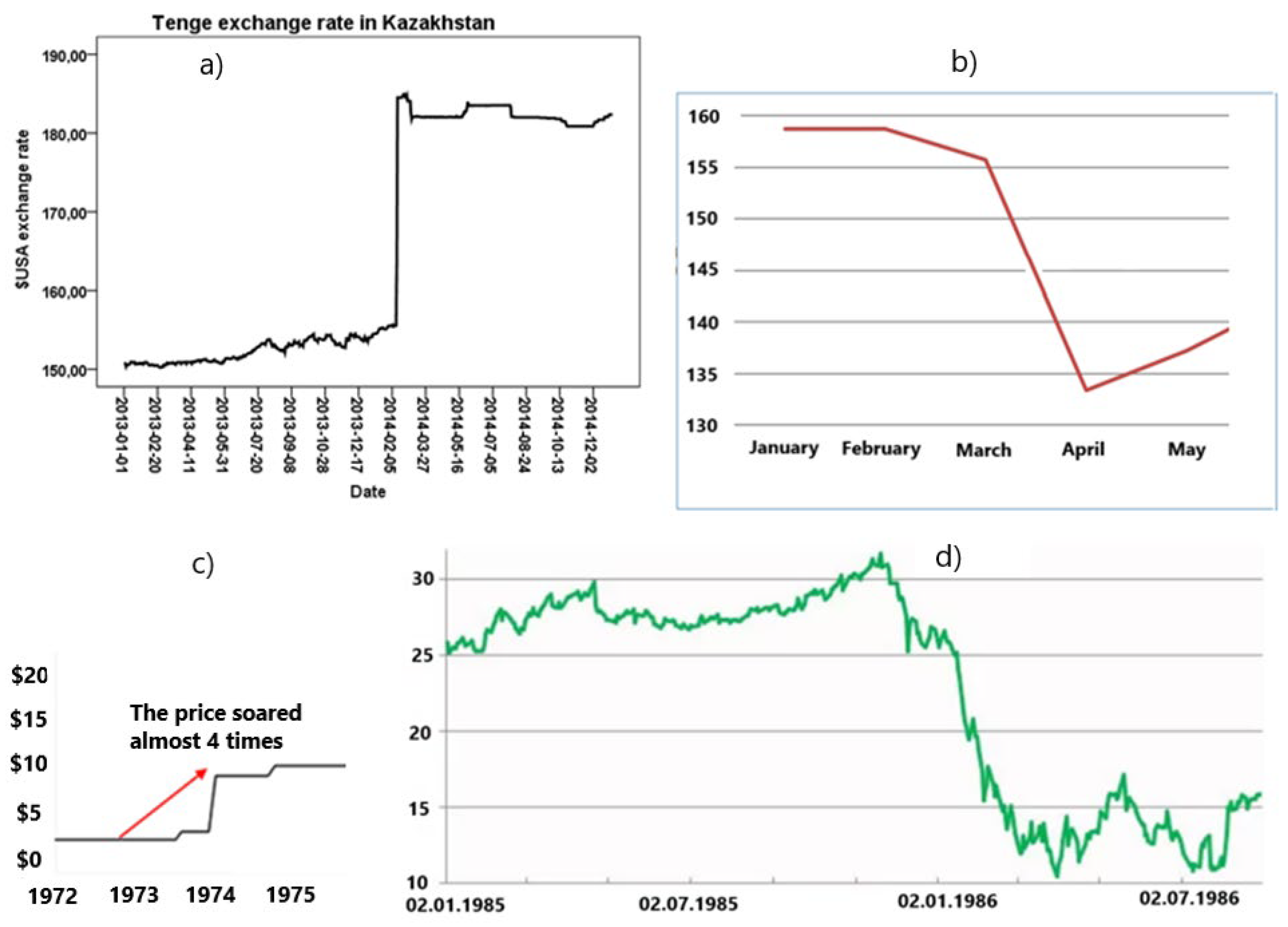
Figure 3.
Graph of the smoothed average for the change in the tenge exchange rate.
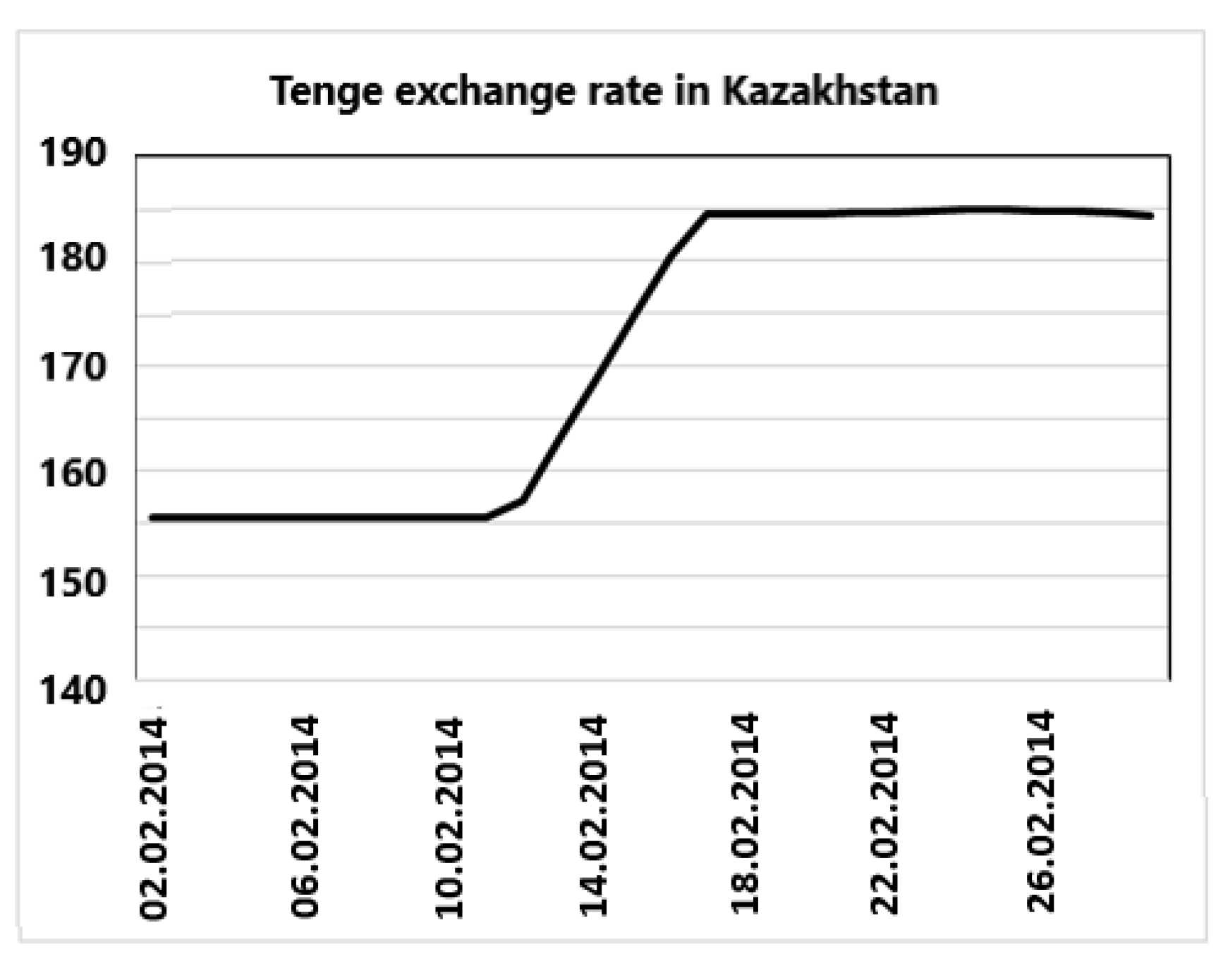
Figure 4.
Graphs of impulse functions.
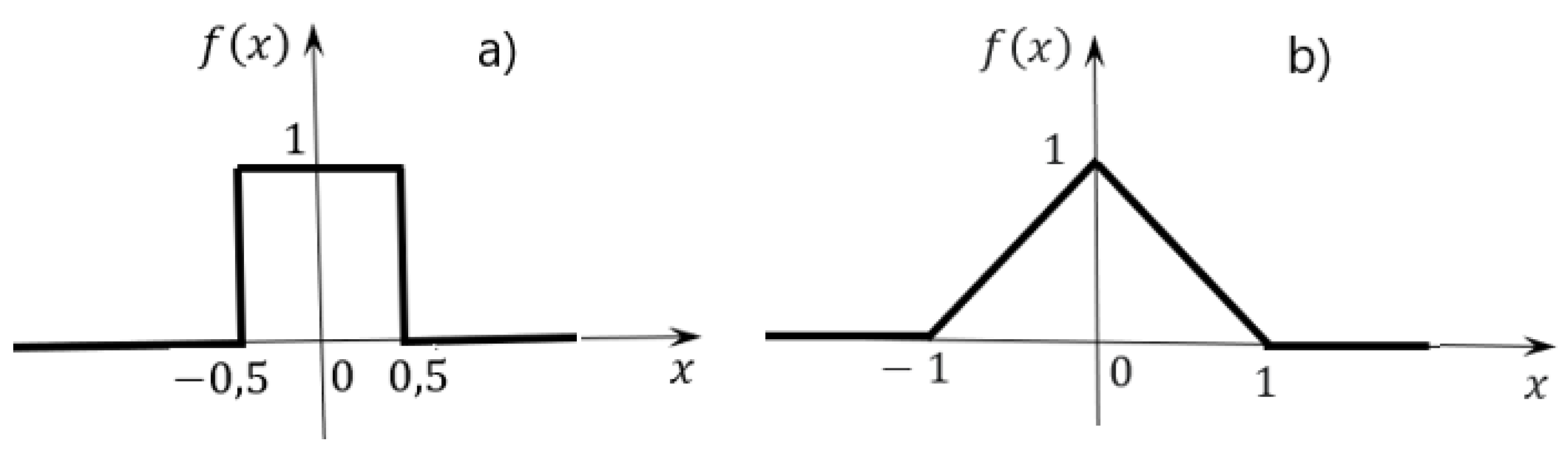
Figure 5.
Examples of impulse changes in the economy: a) monthly change in employment level in the USA, source: US Bureau of Labor Statistics; b) Dow Jones industrial index, source: https://www.economicportal.ru/ponyatiya-all/makroekonomicheskij-shok.html; c) dynamics of real money supply in Russia, source: Central Bank of Russia, Rosstat; d) inflation in Russia, source: Rosstat data.
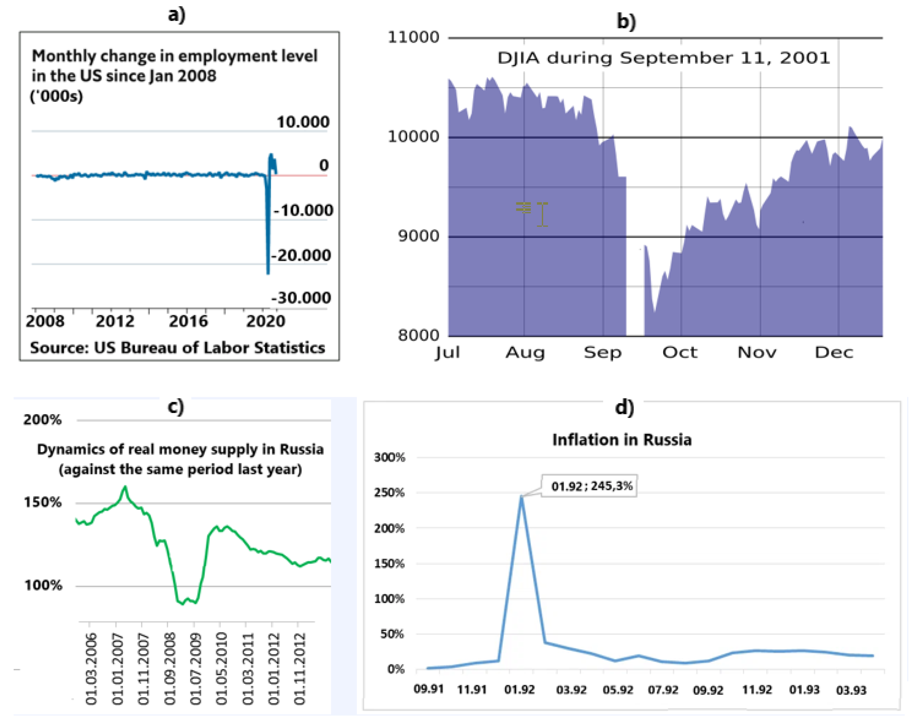
Figure 6.
The exchange rate of the Russian ruble against the US dollar.
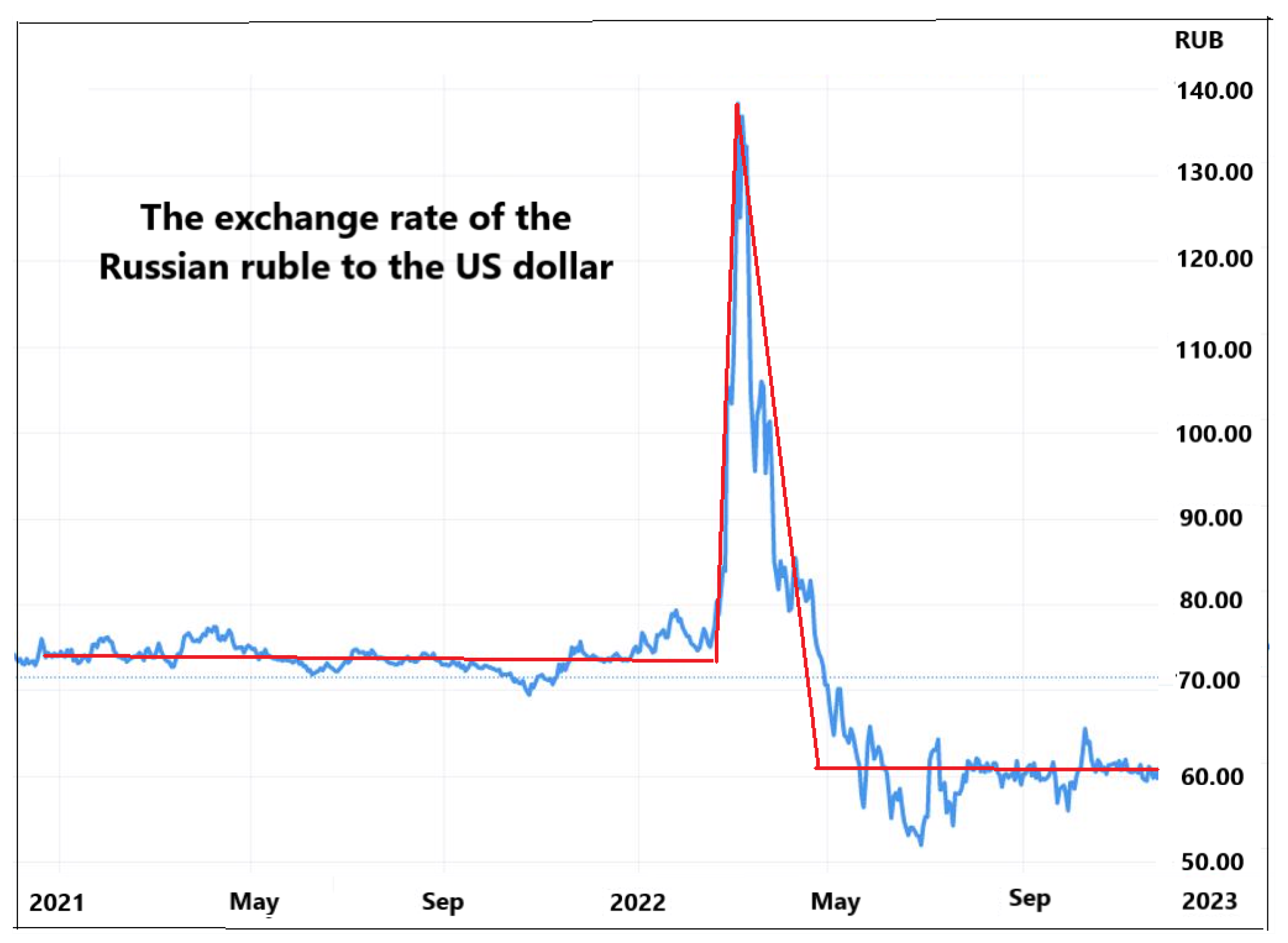
Figure 7.
Dynamics of the world cycle: industrial production, 2019–2022, seasonally adjusted quarterly growth rates. Source: Federal Reserve Economic Data.
Figure 7.
Dynamics of the world cycle: industrial production, 2019–2022, seasonally adjusted quarterly growth rates. Source: Federal Reserve Economic Data.
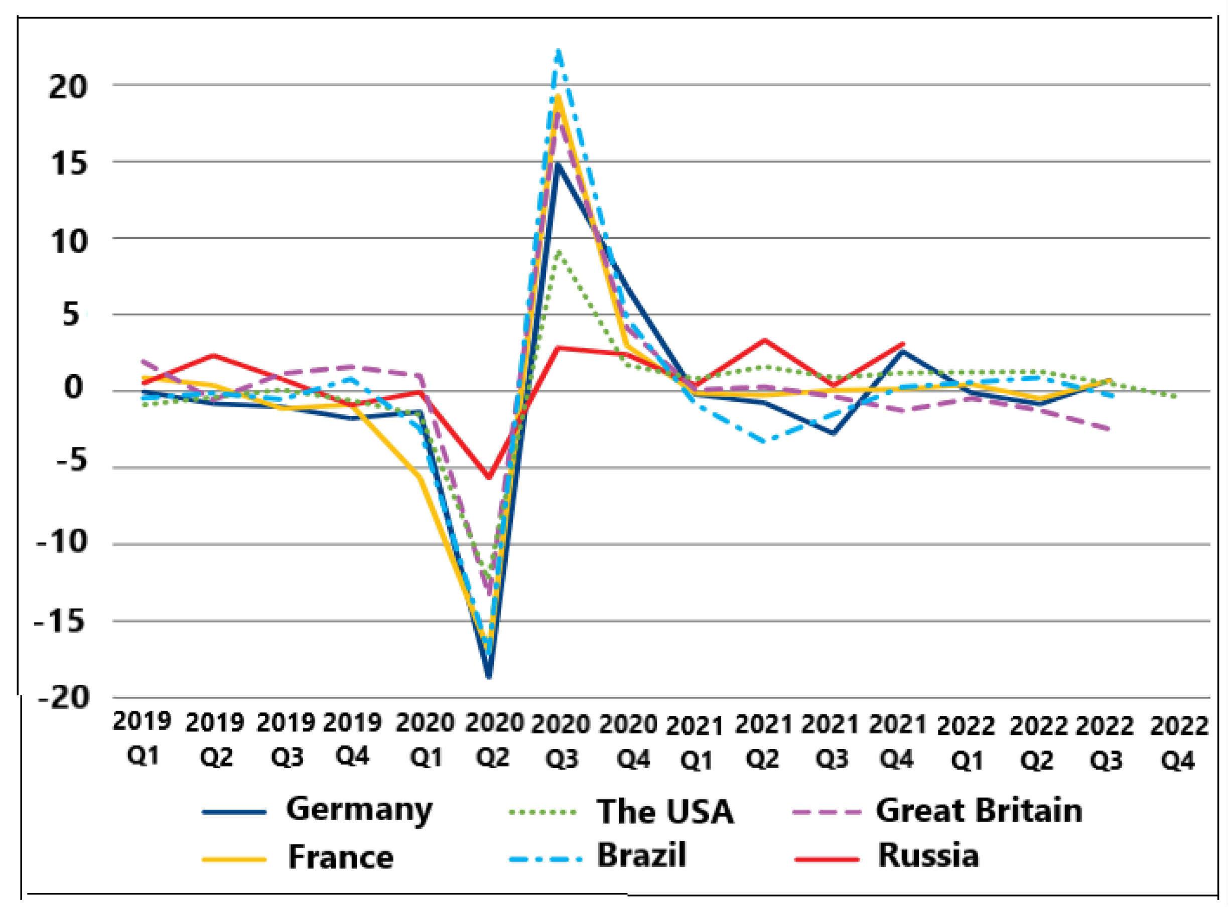
Figure 8.
Graphs of the step function (the thick line) and five successive approximations of this function (the thin lines).
Figure 8.
Graphs of the step function (the thick line) and five successive approximations of this function (the thin lines).
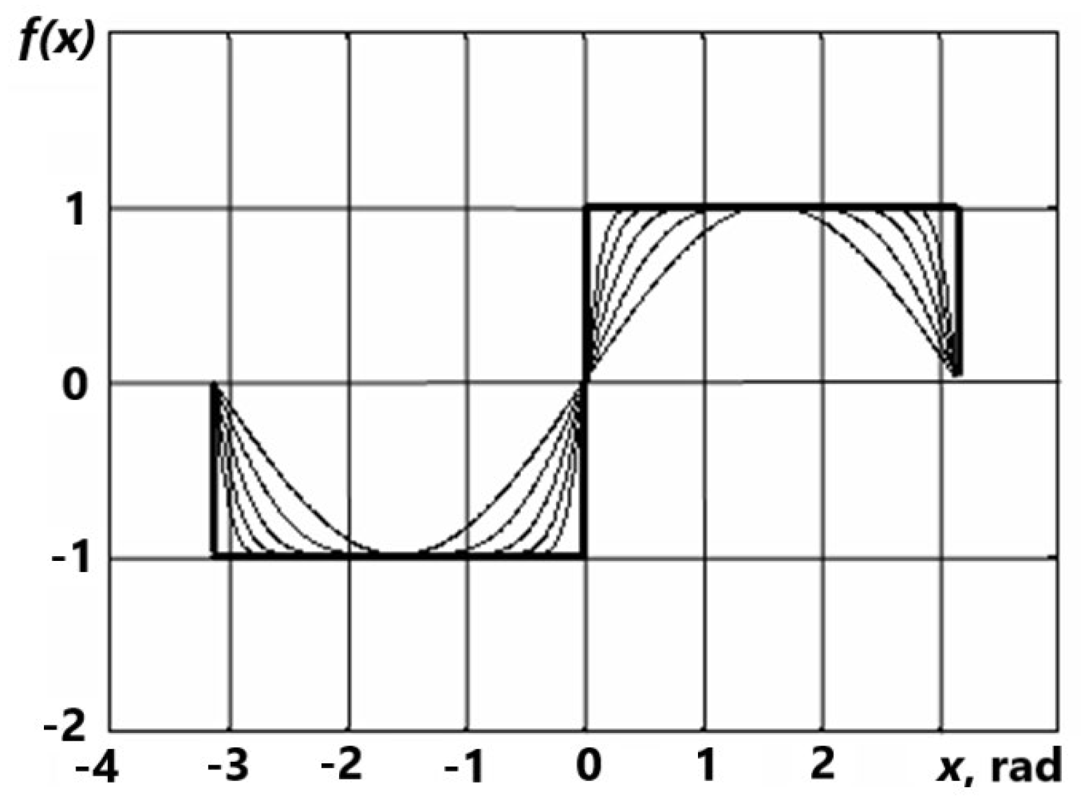
Figure 9.
Graphs of successive approximations of the bar function.
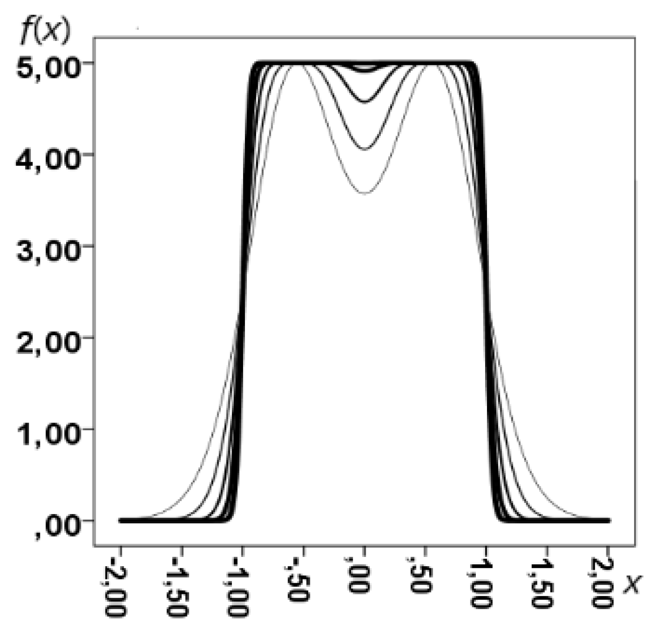
Figure 10.
Graph of step function.
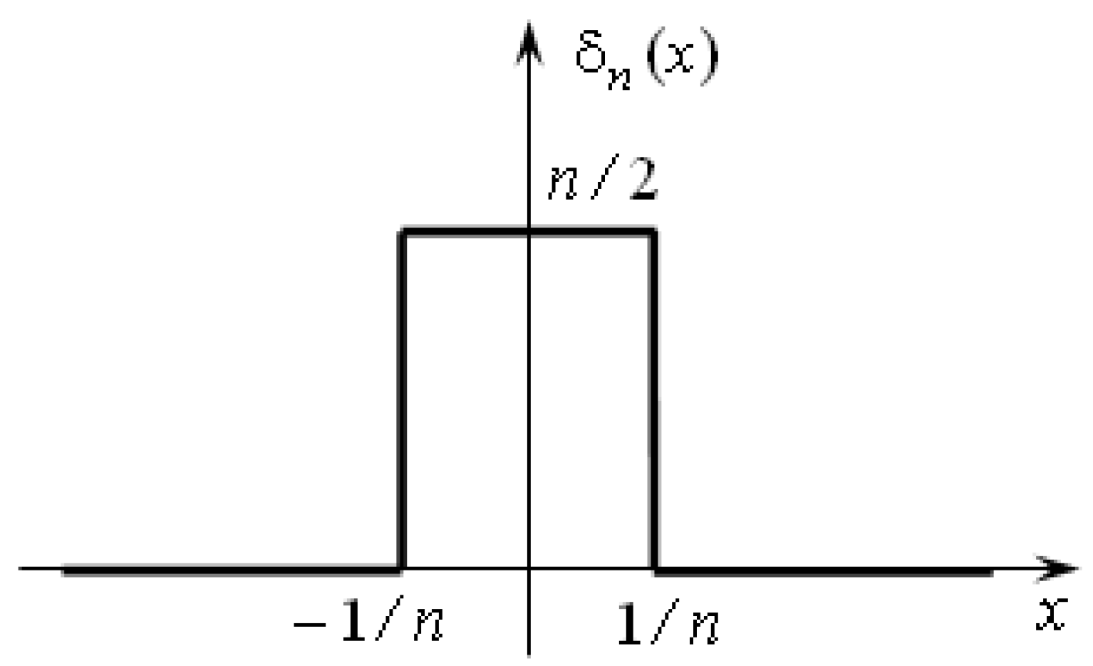
Figure 11.
Graph one of the approximations for δ - functions.
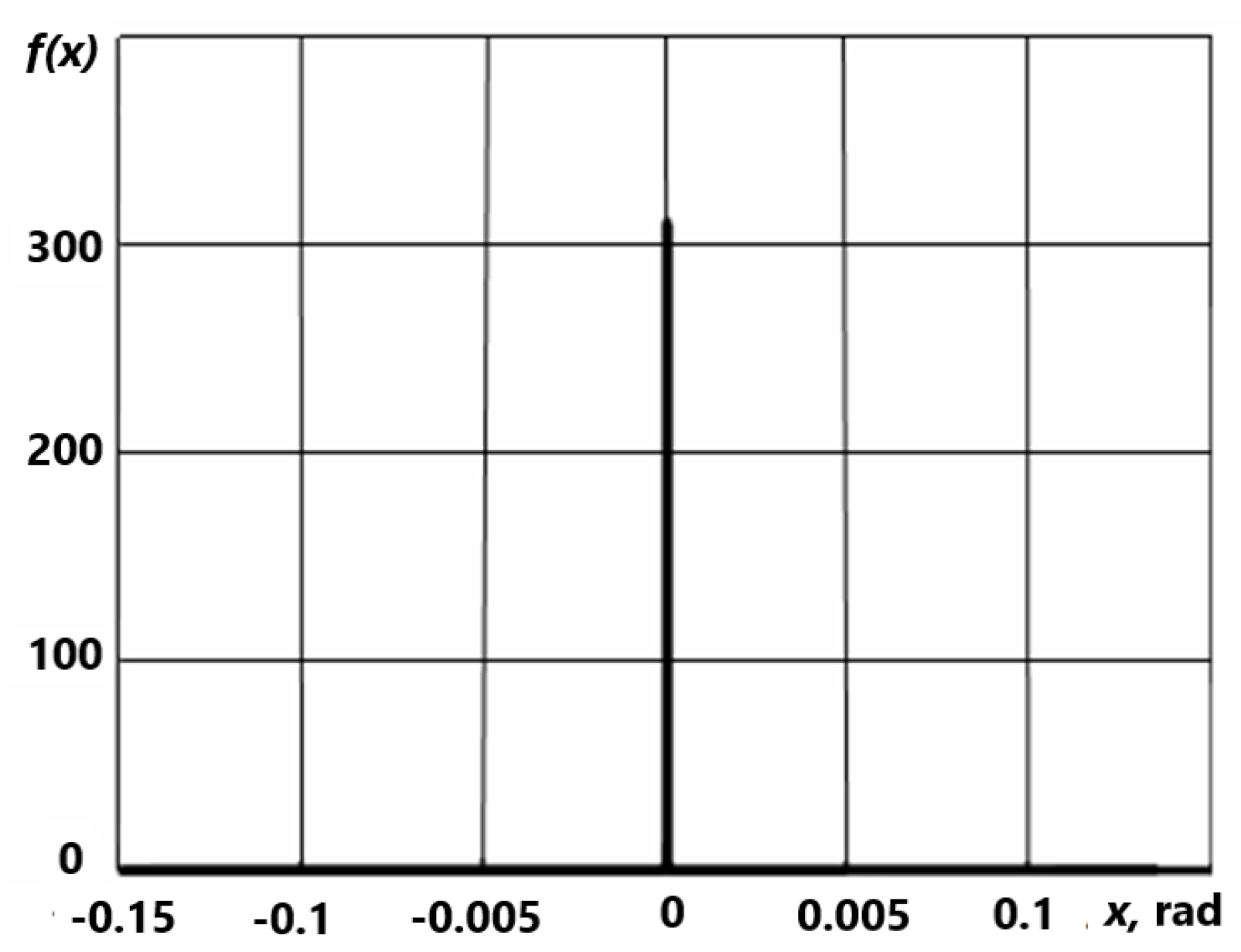
Figure 12.
Graphs of approximations of the Heaviside function.
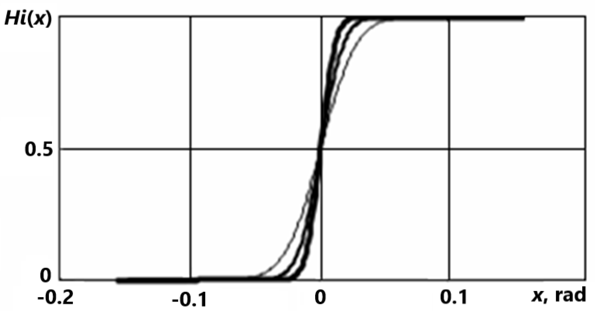
Figure 13.
Graphs of approximations for δ - function.
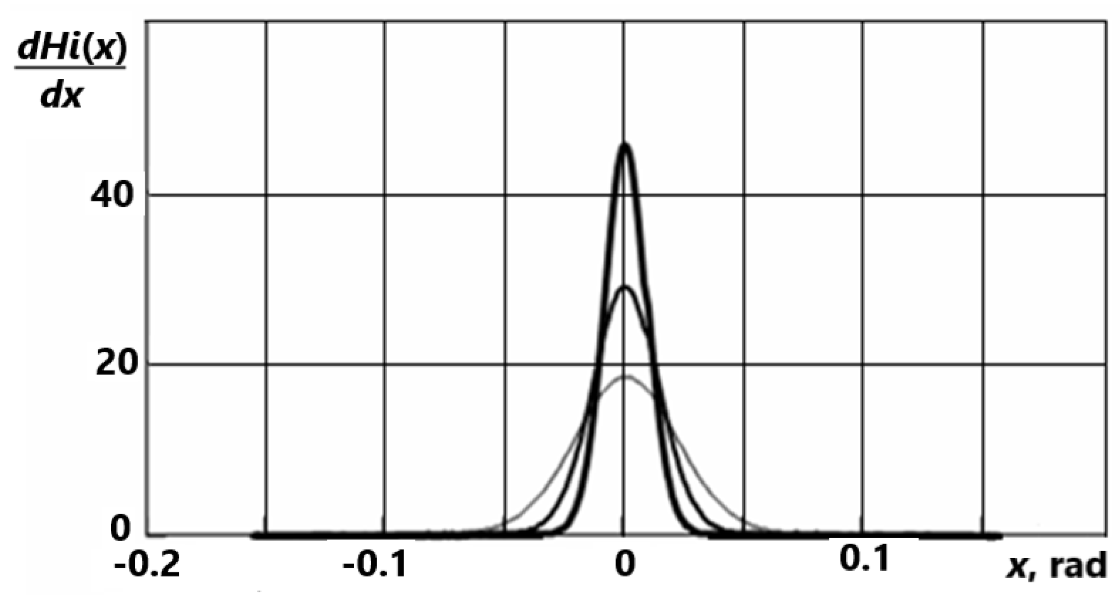
Figure 14.
Graphs of the data set in the range: a) 3σ and b) 4σ.
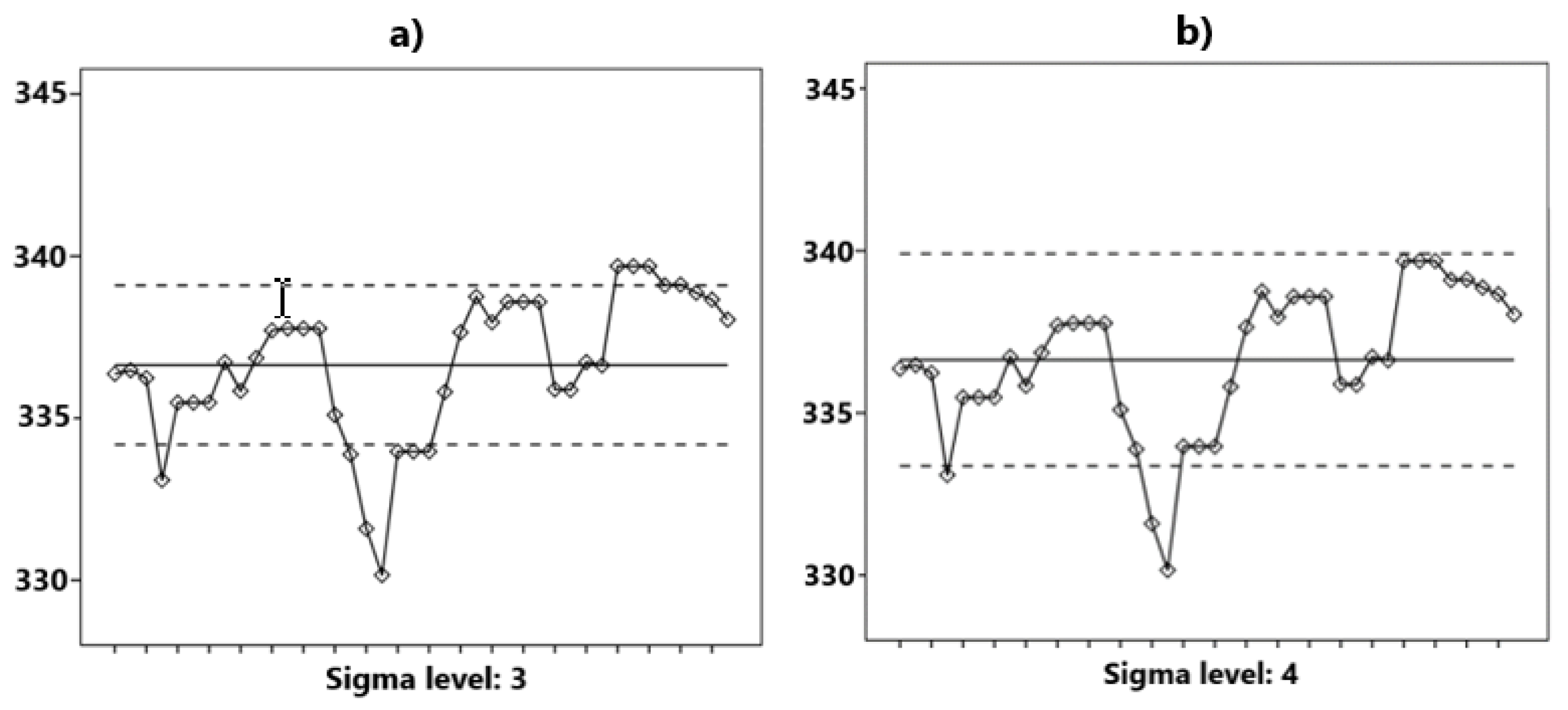
Figure 15.
Examples of completed forecasts: a) Brent oil price; b) Inflation in Russia by months.
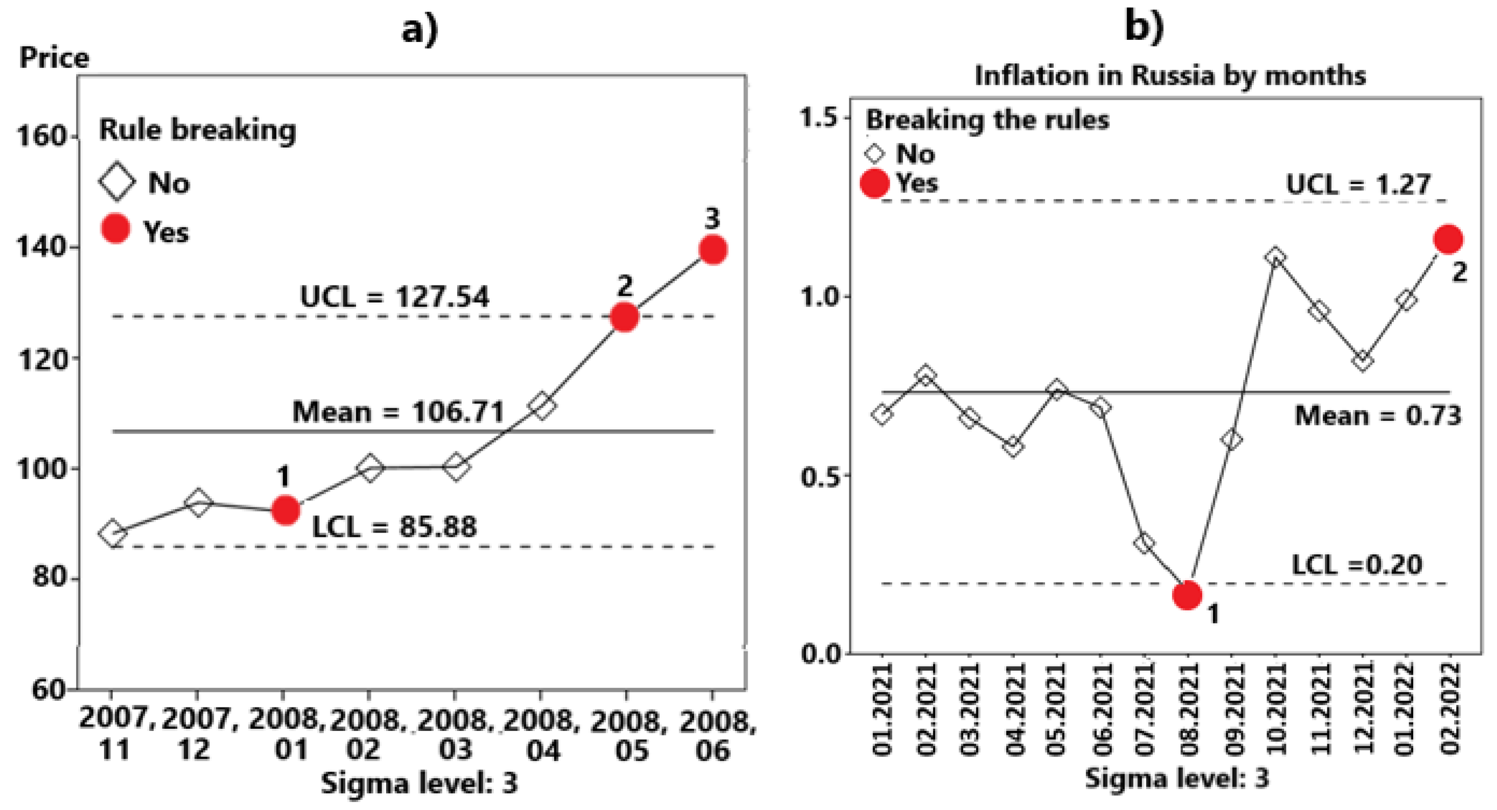
Figure 16.
Schedule of the average monthly salary.
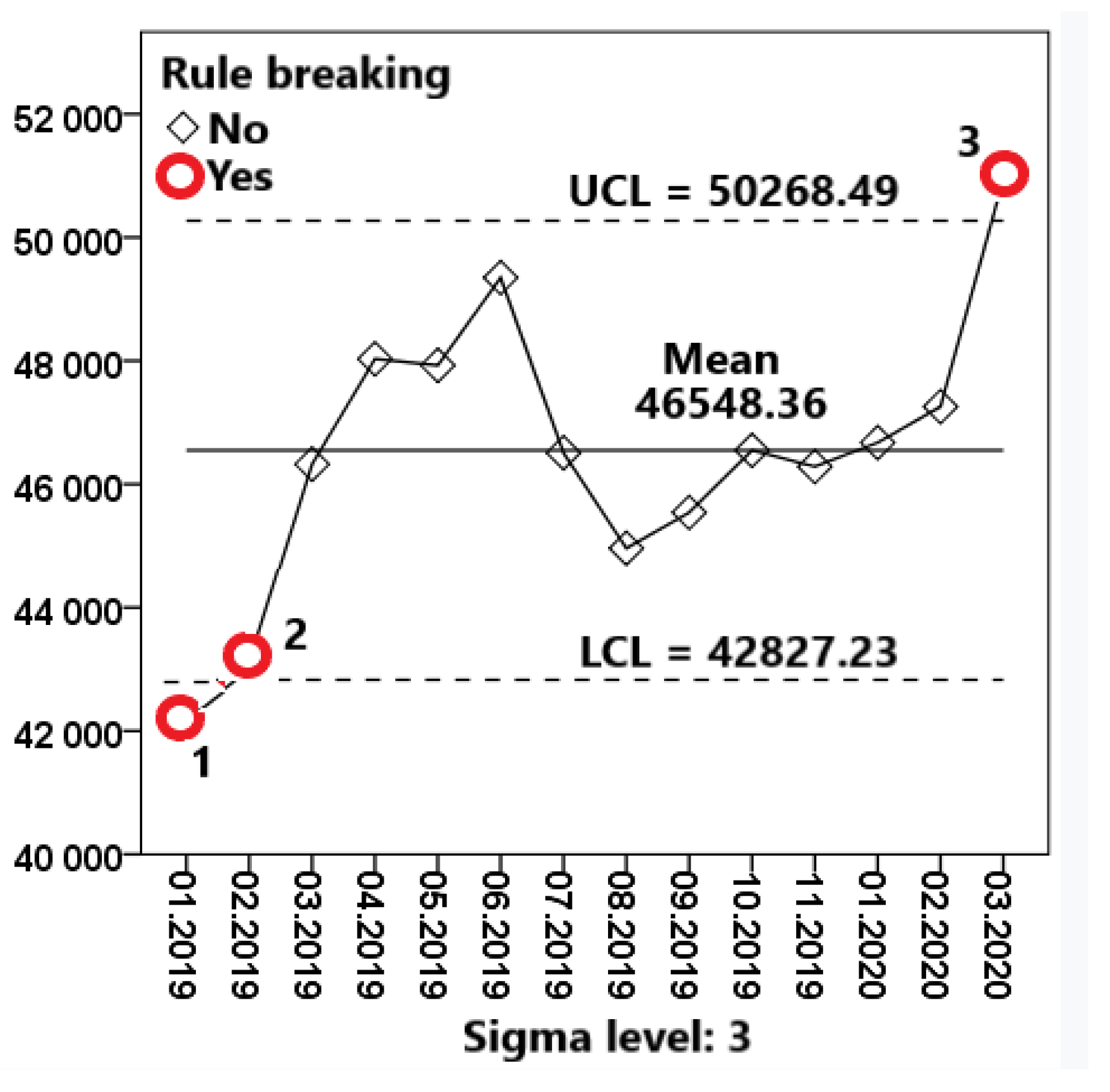
Figure 17.
Visual representation of multidimensional information: a) multidimensional scaling; b) cluster analysis dendrogram.
Figure 17.
Visual representation of multidimensional information: a) multidimensional scaling; b) cluster analysis dendrogram.
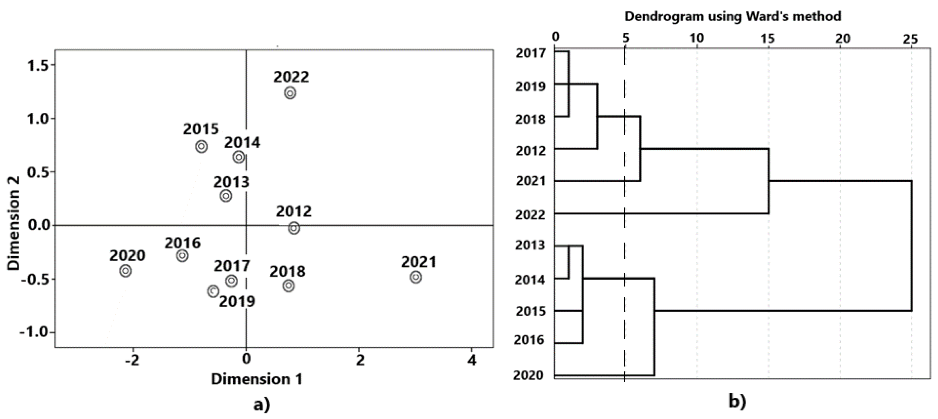
Figure 18.
Graphical representation of the results of multivariate scaling.
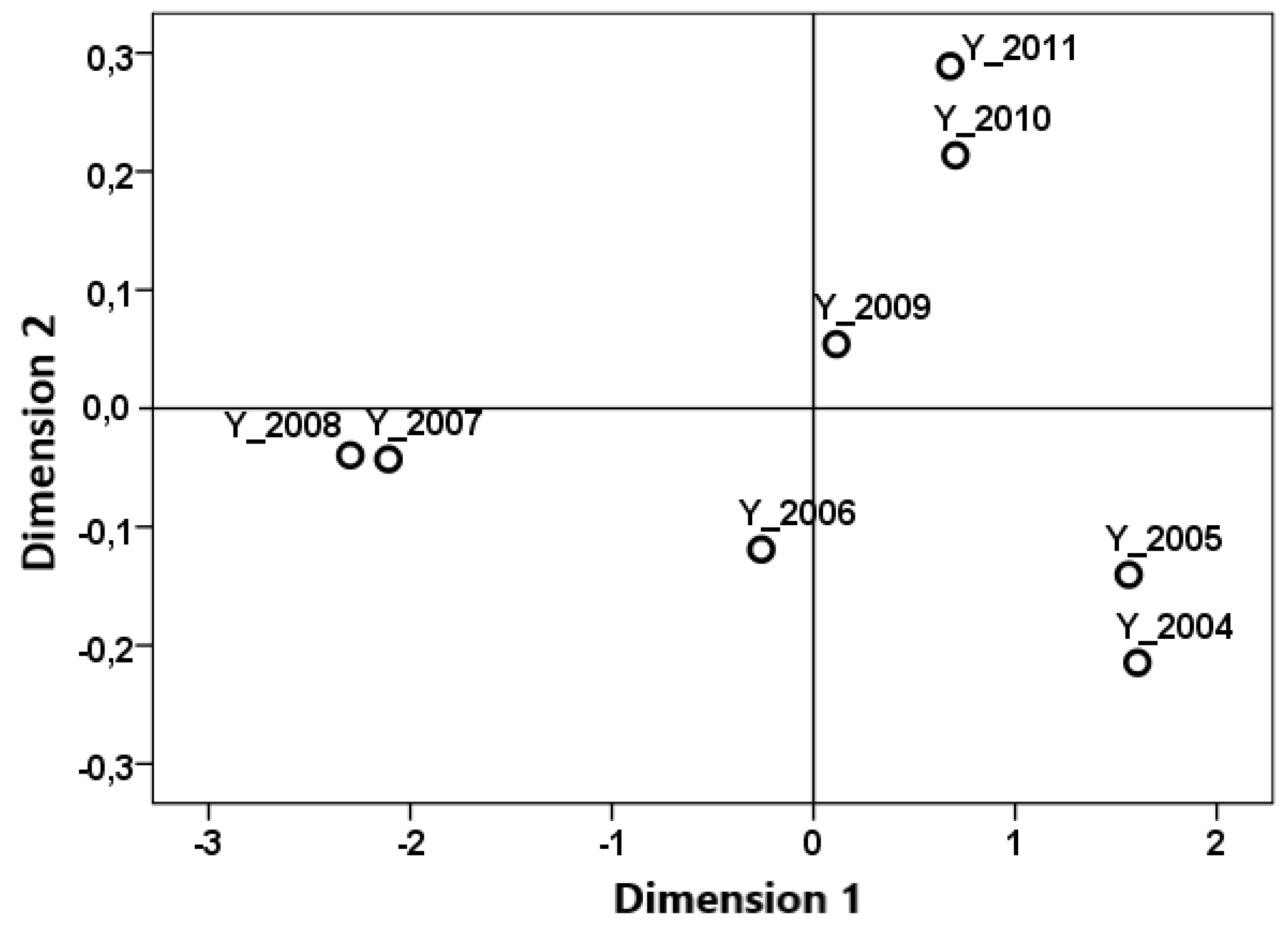

Table 1.
Exchange rates in Kazakhstan.
| Date | Dollar exchange rate | Euro exchange rate |
| 2014-02-10 | 155,5 | 210,89 |
| 2014-02-11 | 155,56 | 212,25 |
| 2014-02-12 | 163,9 | 224,07 |
| 2014-02-13 | 184,5 | 251,57 |
Table 2.
The macroeconomic parameters.
| Main Indicators | Additional Indicators |
|
|
|
|
|
|
|
|
|
|
|
|
|
|
|
|
|
|
|
|
|
|
|
|
|
|
|
|
|
Table 3.
Brent oil price.
| Date | 07.07.2023 | 06.07.2023 | 05.07.2023 | 04.07.2023 | 03.07.2023 |
| Price, $US per barrel | 78,47 | 76,52 | 76,65 | 76,25 | 74,65 |
Table 4.
Control rules.
| Values above + 3 sigma | Values below are 3 sigma |
| 2 of last 3 above + 2 sigma | 2 of the last 3 below are 2 sigma |
| 4 of last 5 above + 1 sigma | 4 of the last 5 below are 1 sigma |
| 8 points in a row above the center line | 8 points in a row below the center line |
| 6 points in a row ascending | 6 points in a row descending |
| 14 points in a row alternately | |
Table 5.
Dynamics of oil prices.
| Date | Violations for points |
| January 2008 | 2 points from the last 3 below - 2 sigma |
| May 2008 | Greater than + 3 sigma |
| June 2008 | Greater than + 3 sigma |
| June 2008 | 2 points from last 3 above + 2 sigma |
| June 2008 | 6 points in a row ascending |
Table 6.
Average monthly salary in rubles.
|
01. 2019 |
02. 2019 |
03. 2019 |
04. 2019 |
05. 2019 |
06. 2019 |
07. 2019 |
08. 2019 |
09. 2019 |
10. 2019 |
11. 2019 |
01. 2020 |
02. 2020 |
03. 2020. |
| 42263 | 43062 | 46324 | 48030 | 47926 | 49348 | 46509 | 44961 | 45541 | 46549 | 46285 | 46674 | 47257 | 50948 |
Table 7.
Violation of control rules.
| Date | Violations for points |
| 01.2019 | Less than -3 sigma |
| 02.2019 | 2 points from the last 3 below - 2 sigma |
| 03.2020 | Greater than + 3 sigma |
Table 8.
Dynamics of macroeconomic indicators of Russia for the period 2012-22.
| Year | GDP growth at current prices, % | Unemployment rate, % | Industrial production index in % of the previous year | Consumer price indices for services at the end of the period, in % to December of the previous year | Labor productivity index in the economy in % of the previous year |
| 2012 | 13,3 | 5,5 | 103,4 | 107,28 | 103,8 |
| 2013 | 7,2 | 5,5 | 100,4 | 108,01 | 102,1 |
| 2014 | 8,3 | 5,2 | 101,7 | 110,45 | 100,8 |
| 2015 | 5,1 | 5,6 | 100,2 | 110,20 | 98,7 |
| 2016 | 3,0 | 5,5 | 101,8 | 104,89 | 100,1 |
| 2017 | 7,3 | 5,2 | 103,7 | 104,35 | 102,1 |
| 2018 | 13,1 | 4,8 | 103,5 | 103,94 | 103,1 |
| 2019 | 5,5 | 4,6 | 103,4 | 103,75 | 102,4 |
| 2020 | -1,8 | 5,8 | 97,9 | 102,70 | 99,6 |
| 2021 | 25,7 | 4,8 | 105,3 | 104,98 | 103,7 |
| 2022 | 13,4 | 3,9 | 99,4 | 113,19 | 102.8 |
Table 9.
Clustering.
| Year | 2012 | 2013 | 2014 | 2015 | 2016 | 2017 | 2018 | 2019 | 2020 | 2021 | 2022 |
| Cluster | 1 | 2 | 2 | 2 | 2 | 1 | 1 | 1 | 3 | 4 | 5 |
Table 10.
Mean values of variables by clusters.
| Ward Method | GDP growth at current prices, % | Unemployment rate, % | Industrial production index in % of the previous year | Consumer price indices for services at the end of the period, in % to December of the previous year | Labor productivity index in the economy in % of the previous year | |
| 1 | Mean | 9,8000 | 5,0250 | 103,5000 | 104,8300 | 102,8500 |
| N | 4 | 4 | 4 | 4 | 4 | |
| 2 | Mean | 5,9000 | 5,4500 | 101,0250 | 108,3875 | 100,4250 |
| N | 4 | 4 | 4 | 4 | 4 | |
| 3 | Mean | -1,8000 | 5,8000 | 97,9000 | 102,7000 | 99,6000 |
| N | 1 | 1 | 1 | 1 | 1 | |
| 4 | Mean | 25,7000 | 4,8000 | 105,3000 | 104,9800 | 103,7000 |
| N | 1 | 1 | 1 | 1 | 1 | |
| 5 | Mean | 13,4000 | 3,9000 | 99,4000 | 113,1900 | 102,8000 |
| N | 1 | 1 | 1 | 1 | 1 | |
| Total | Mean | 9,1000 | 5,1273 | 101,8818 | 106,7036 | 101,7455 |
| N | 11 | 11 | 11 | 11 | 11 | |
Table 11.
Dynamics of the main macroeconomic indicators of Russia in 2004-2011 (growth rate, %). Source: Rosstat and Bank of Russia.
Table 11.
Dynamics of the main macroeconomic indicators of Russia in 2004-2011 (growth rate, %). Source: Rosstat and Bank of Russia.
| Years | 2004 | 2005 | 2006 | 2007 | 2008 | 2009 | 2010 | 2011 |
| Unemployment | 7.9 | 7.6 | 6.9 | 6.1 | 6.4 | 8.6 | 7.6 | 7.3 |
| Inflation, December to December | 11.7 | 10.9 | 9.0 | 9.3 | 13.0 | 8.8 | 7.4 | 6.3 |
| Gross domestic product | 7.2 | 6.4 | 6.7 | 8.1 | 5.6 | -7.9 | 4.0 | 4.1 |
| Industrial products | 8.3 | 4.0 | 4.9 | 6.1 | 2.1 | -10.8 | 8.3 | 4.1 |
| Agricultural products | 3.0 | 2.4 | 3.6 | 3.3 | 1.8 | -5.5 | -2.3 | 7.4 |
| Real disposable income of the population | 10.4 | 11.1 | 10.0 | 10.7 | 2.9 | 1.1 | 3.5 | 4.2 |
| Retail turnover | 13.3 | 12.8 | 13.0 | 15.9 | 13.2 | -5.0 | 4.5 | 4.8 |
| Gold and foreign exchange reserves of the Central Bank (billion US dollars) | 130.0 | 175.0 | 300.0 | 479.4 | 426.3 | 439.0 | 500.2 | 585.8 |
| Volume of the stabilization fund (billion rubles) | 489.0 | 522.3 | 2180.0 | 3859.0 | 4027.6 | 1830.5 | 1279.9 | 1300.0 |
| Investments in fixed assets | 11.7 | 10.5 | 13.5 | 20.3 | 9.8 | -11.0 | 5.9 | 9.0 |
| World oil price (Urals) | 34.4 | 50.6 | 61.1 | 69.3 | 94.4 | 61.1 | 78.2 | 90.0 |
| Export of goods, billion US dollars | 183.2 | 243.6 | 304.5 | 355.5 | 471.6 | 304.0 | 400.4 | 380.4 |
| Import of goods, billion US dollars | 97.4 | 125.3 | 163.9 | 223.4 | 291.9 | 192.0 | 248.7 | 250.1 |
Disclaimer/Publisher’s Note: The statements, opinions and data contained in all publications are solely those of the individual author(s) and contributor(s) and not of MDPI and/or the editor(s). MDPI and/or the editor(s) disclaim responsibility for any injury to people or property resulting from any ideas, methods, instructions or products referred to in the content. |
© 2023 by the authors. Licensee MDPI, Basel, Switzerland. This article is an open access article distributed under the terms and conditions of the Creative Commons Attribution (CC BY) license (http://creativecommons.org/licenses/by/4.0/).
Copyright: This open access article is published under a Creative Commons CC BY 4.0 license, which permit the free download, distribution, and reuse, provided that the author and preprint are cited in any reuse.


