Price oligopoly with differentiated product and dependence of total demand on the bottom price

Preprint

Article

Price oligopoly with differentiated product and dependence of total demand on the bottom price

Altmetrics

Downloads

128

Views

Comments

Alexander Filatov^*

This version is not peer-reviewed

Submitted:

17 October 2023

Posted:

19 October 2023

You are already at the latest version

Alerts

Abstract

The paper proposes a game theory model of price oligopoly with a heterogeneous product, where total demand depends linearly on the minimum market price. This model develops the Bertrand oligopoly for the case of imperfect price elasticity of demand. The most interesting result is an asymmetric Nash equilibrium with different prices and sales in the situation of symmetric oligopolists. The asymmetry is explained by the fact that a decrease in the minimum market price leads not only to a reallocation of consumers among firms, but also to an increase in total demand. Modifications of a two-stage game with a leader and followers and the price discrimination model are also considered. Microeconomic substantiation of the model is given on the basis of the spatial differentiation approach.

Keywords:

Subject: Business, Economics and Management - Economics

MSC: 91B24; 91A40; 91A80; 91B72

1. Introduction

Oligopoly is the most common and most interesting (due to the huge number of non-trivial strategies of participants’ behavior) type of industrial markets. Even if we face several dozen companies at a market, usually the core consists of 2-10 biggest producers that take into account behavior of big rivals and competitive fringe. The classical approach to model such markets was proposed in seminal works of Cournot [1], Bertrand [2], and Stackelberg [3]. But all of them deal with a homogeneous product, which is not realistic for most markets, especially in recent decades. Indeed, in most modern industries the products of different producers are not identical for consumers. Even if the physical properties are barely distinguishable, then branding, additional services, spatial distribution make the products differentiated [4].

There are two most popular demand models that take into account the product differentiation. The first one was proposed in the book of Bowley [5], and after extensions of Dixit [6], and Singh, Vives [7] became a standard tool for oligopoly analysis. For duopoly the inverse demand system is derived from the following utility maximization problem:

\{\begin{cases} u_{1} (q_{0}, q_{1}, q_{2}) = α q_{1} + α q_{2} - \frac{β q_{1}^{2} + 2 γ q_{1} q_{2} + β q_{2}^{2}}{2} + q_{0} \to \max, \\ q_{0} + p_{1} q_{1} + p_{2} q_{2} = y, \end{cases}

and takes the following form:

\{\begin{cases} p_{1} = M U_{1} = α - β q_{1} - γ q_{2}, \\ p_{2} = M U_{2} = α - γ q_{1} - β q_{2} . \end{cases}

Here y denotes the total consumer budget, spending on two products purchasing in quantities q₁ and q₂ at prices p₁ and p₂. q₀ is the remaining amount of money. Coefficients α and β are always positive, and γ is positive for substitution goods, which we will study in the paper, and negative for complements. The ratio δ =γ²/β² can serve as a measure of differentiation. It always less than one, but γ→β for perfect substitutes, and γ=0 for independent goods. The main options of the Bowley-Singh-Vives model are presented in Figure 1.

The model can be inverted and reduced to the following form:

\{\begin{cases} q_{1} = a - b p_{1} + c p_{2}, \\ q_{2} = a + c p_{1} - b p_{2}, \end{cases}

(1)

where

a = α \frac{β - γ}{β^{2} - γ^{2}}, b = \frac{β}{β^{2} - γ^{2}}, c = \frac{γ}{β^{2} - γ^{2}} .

Thus, it is possible to obtain a non-degenerate equilibrium not only in the framework of the Cournot quantitative oligopoly, but also in the Bertrand price oligopoly.

The alternative approach to model demand system in oligopoly was proposed by Shapley and Shubik [8]. It is based on the following maximization problem:

\{\begin{cases} u_{2} (q_{0}, q_{1}, q_{2}) = α q_{1} + α q_{2} - \frac{β (q_{1}^{2} + q_{2}^{2}) - γ {(q_{1} - q_{2})}^{2}}{2} + q_{0} \to \max, \\ q_{0} + p_{1} q_{1} + p_{2} q_{2} = y, \end{cases}

which solution looks like

\{\begin{cases} p_{1} = M U_{1} = α - (β - γ) q_{1} - γ q_{2}, \\ p_{2} = M U_{2} = α - γ q_{1} - (β - γ) q_{2} . \end{cases}

When we are dealing with independent goods (with γ=0) both models are identical. Moreover, it seems that the models are generally the same up to parameter designations. But it is not so. If we change parameter γ, related to cross effects, in the Bowley-Singh-Vives model, the impact of output on own price doesn’t change. On the contrary, in the Shapley-Shubik model increase in price dependence on foreign output (which implies greater substitutability of goods) also increases the dependence of demand on own price which implies increased competition.

It is especially important when studying investments in innovation [9] as well as when analyzing the strategic choice of the product differentiation level carried out by firms [10]. A detailed comparison of the two presented approaches is carried out by Thielen in [11].

Nevertheless, both approaches don’t take into account at least one feature. In both models the total market demand depends equally on price changes in both cheap and expensive firms. In reality the expansion of the market and the influx of new consumers occurs mainly with a decrease in the bottom price (the lowest among the prices of all producers). Price reduction in more expensive firms does not increase total sales, but only redistributes demand in their favor. This feature leads to asymmetry in optimal behavior and asymmetric equilibrium even in situation of cost-homogeneous firms.

It’s not just a theoretical concept. We can see asymmetric pricing policies in practice. It is usually associated either with the heterogeneity of retailers in terms of costs, or with vertical differentiation, as in Gabszewicz, Thisse [12] and Shaked, Sutton [13] papers, where firms choose the quality of the product at the first stage, and the price at the second stage. But such models can’t explain, why even similar retailers with similar costs charge significantly different prices for identical products.

Today there is a sale in one retail chain, while in the rest the product is sold much more expensive. Tomorrow the retailers will change places. Is it inefficiency, some behavioral artefact, or such situation has same rational explanation? Sometimes it’s possible to apply here concepts of economics of information. Hal Varian [14] finds the cause of intertemporal price dispersion in uninformed buyers who purchase products not in the cheapest, but in a random place, and profit maximizing retailers can exploit this. Nevertheless, this is not the only explanation. Asymmetric equilibrium arises even if consumers have complete information about prices.

We’ll construct the formal model in the section 2 of the paper. The section 3 contains the microeconomic substantiation of the model based on the concepts of spatial differentiation. In the section 4 we analyze the emerging equilibrium and its properties. The sections 5-7 are devoted to some modifications of the basic model – the problem of inversion, two-stage leader-follower game, cartel and price discrimination case. And the section 8 finalize the paper with discussion, some conclusions and policy implications.

2. The Model

Let’s consider a market consisting of n identical producers with marginal costs c. To begin with, we assume that the fixed total demand in the market is equal to Q. If all firms set the same price, demand is divided equally among them, amounting to Q/n. If the price in j-firm increases by each dollar, its quantity decreases by x, while quantity of rivals increases by x/(n–1). Thus, the demand function takes the form q=Q/n + Xp, where

q = (\begin{matrix} q_{1} \\ q_{2} \\ q_{3} \\ ... \\ q_{n} \end{matrix}), p = (\begin{matrix} p_{1} \\ p_{2} \\ p_{3} \\ ... \\ p_{n} \end{matrix}), Q = (\begin{matrix} Q \\ Q \\ Q \\ ... \\ Q \end{matrix}), X = (\begin{matrix} - x & \frac{x}{n - 1} & \frac{x}{n - 1} & ... & \frac{x}{n - 1} \\ \frac{x}{n - 1} & - x & \frac{x}{n - 1} & ... & \frac{x}{n - 1} \\ \frac{x}{n - 1} & \frac{x}{n - 1} & - x & ... & \frac{x}{n - 1} \\ ... & ... & ... & ... & ... \\ \frac{x}{n - 1} & \frac{x}{n - 1} & \frac{x}{n - 1} & ... & - x \end{matrix}),

(2)

The proposed linear formula is the simplest way to explain the symmetric substitution effect – consumers prefer to buy goods in cheaper stores. But it still doesn’t explain market expansion when prices fall. Indeed, due to (2), if any producer decreases price, it just attracts some additional clients from other firms, and vice versa, an increase in price causes some customers to switch to rivals, but total sales in a market remain unchanged.

It’s easy to believe that something similar happens in real markets when we consider price changes in expensive firms. Indeed, lowering the price of a certain good from $100 to $80 in an expensive firm may attract some wealthy customers who had previously been served by cheaper rivals selling it for $50, but is unlikely to interest those who are unable to pay even $50. Also airline sale of business class tickets will allow it to sell some seats to people who usually fly economy, but not to people who can’t afford to travel at all.

On the contrary, a sale reducing the price from $50 to $30 in a cheap firm will not only lure some customers from other firms, but also expand demand to a new audience. And the sale conducted by low-cost carrier significantly expands the total demand in the market. Thus price reduction in a low-cost firm should affect quantity.

Let’s assume that total market demand Q = q₁+…+q_n depends only on the “bottom price” p₁, the minimum among the prices of all producers:

Q = a – bp₁, p₁ = min {p₁, p₂, …, p_n}.

(3)

Note that we renumber the firms to make the first one the cheapest. Of course, to set the demand in such a way is also a simplification of the situation, but it is closer to reality than using classical formulas (1).

If we redefine x = bΔ, and substitute (3) into (2), than the demand vector-function takes the following form:

q = a / n + Bp, a = (\begin{matrix} a \\ a \\ a \\ ... \\ a \end{matrix}), B = (\begin{matrix} - b Δ - \frac{b}{n} & \frac{b Δ}{n - 1} & \frac{b Δ}{n - 1} & ... & \frac{b Δ}{n - 1} \\ \frac{b Δ}{n - 1} - \frac{b}{n} & - b Δ & \frac{b Δ}{n - 1} & ... & \frac{b Δ}{n - 1} \\ \frac{b Δ}{n - 1} - \frac{b}{n} & \frac{b Δ}{n - 1} & - b Δ & ... & \frac{b Δ}{n - 1} \\ ... & ... & ... & ... & ... \\ \frac{b Δ}{n - 1} - \frac{b}{n} & \frac{b Δ}{n - 1} & \frac{b Δ}{n - 1} & ... & - b Δ \end{matrix}) .

(4)

Here Δ is a parameter responsible for comparing the demand expansion and its redistribution among producers. We can call it “Preference for search”. The larger delta value, the stronger buyers react to price changes in firms, look for cheaper stores, and become customers of more favorable ones. On the contrary, if Δ=0, nobody is searching at all, everyone is a loyal customer of his favorite firm regardless of the prices.

Let’s explore the issue of selecting Δ in more detail. In particular, let’s analyze reasonable approaches to formalize the dependence of Δ on the number of firms. The first specification of the model (weak preference for search, Δ≡1) means that consumers have weak response to price differences. More precisely, a change in the price of any firm will lead to a change in its sales, regardless of the number of competitors. At the same time, when the number of firms in the market is large, the impact on each of the competitors becomes small.

Assume, for example, that a firm has one competitor in some market. Let the price increase by a dollar lead to the outflow of 100 clients to this competitor. What happens if the number of competitors turn out to be 2, 3, 5, etc? The outflow will remain exactly the same. It means that 2 competitors will get 100/2=50 additional customers each, but in case of 5 competitors only 100/5=20 customers will transfer to each of them (Figure 2).

The substantive implication of this modification is that increased variety does not provide additional incentives for buyers to consider possible alternatives and find cheaper stores. In particular, this occurs in a situation of quality differentiation when all varieties are orthogonal to each other and switching from the ideal good (e.g., when it becomes too expensive) to any of the substitutes results in the same loss of utility.

The second modification, strong preference for search, Δ=n–1 (the opposite extreme case) assumes strong consumer response to the price difference. Moreover, the consumer reaction increases strongly with the number of firms. Technically this means that the if one of the firms raises the price, then the sales of each competitor increase by a fixed amount, regardless of their number. Consequently, the firm’s own sales change in direct proportion to the number of competitors.

For example, if a firm has only one competitor in a market, and a $1 price increase causes 100 customers to go to that competitor, then 2 competitors will take away 100*2=200 customers from the firm, and 5 competitors will take away as many as half a thousand (Figure 3). This modification can be relevant in the case of spatial differentiation. If it is necessary to change a convenient option for a worse one, a small number of stores means significant transportation costs, while an increase in the number of stores leads to the possible emergence of convenient alternatives that can be found by consumers.

The third, intermediate modification (medium preference for search, Δ=2(n–1)/n) implies, on the one hand, a stronger consumer reaction to a price change of one of the firms when the number of competitors increases, but on the other hand, for a perfect competition the effect is only twice as strong (Δ→2 when n→∞) as in the case of a duopoly (Δ=1 when n=2).

Compared to the two extremes, the third intermediate option seems more relevant to reality. An additional justification for it is the following fact: If all expensive firms have the same pricing policy, and p₂=p₃=…=p_n=p*, then the demand function looks like

q * = (a + b p_{1} - 2 b p *) / n

which is identical to the simple duopoly model. In particular, at any fixed price of a cheap firm, its competitors completely lose the market (q* turns to zero) at the price, independent of their quantity n. It agrees well with empirical data and also turns out to be convenient in the analysis of equilibrium behavioral strategies, which we will study in the Section 4.

3. Microeconomic Substantiation

The most common approach to substantiate demand functions in oligopoly is models of spatial differentiation, which originate from the work of Harold Hotelling [15]. Hotelling announced the principle of minimal differentiation, stating that stores in a linear city will be concentrated in its center. Several researchers [16] refuted this rather controversial result. In particular, it is not fulfilled due to the firms’ desire for market power and minimization of price competition, which becomes stronger when stores are clustered, as shown by Claude Aspremont, Jaskold Gabszewicz, and Jacques Thisse in [17].

Nevertheless, the basic principles of Hotelling’s model are still used today, including in the construction of more complex models with different other assumptions. In particular, many researchers often abandon the constraints of the linear city and move to the circular city model [18] or generally to a more realistic two-dimensional space [19]. In some papers the space is no longer geographical. For example, one can study the clustering of consumers in the space of tastes. Such a setting often arises when analyzing the impact of informative [20] and persuasive [21] advertising on consumers. Another application of Hotelling-type models of spatial differentiation is political competition. In 1957 Anthony Downs proposed a model [22] of two strategic (i.e., concerned only with winning elections) parties competing in a one-dimensional political space for the votes of honest voters who vote for the political platform closest to their own.

Hotelling’s principles are equally applicable to demand estimation both in classical deterministic game theory models as well as in discrete choice models [23], the empirics of which is explored in a study [24]. We will also use these principles, assuming that the total cost of a good is made up of its price and heterogeneous transportation costs associated with the distance from the customer’s home to the store.

So let’s assume that there are two firms located at different ends of a linear city, specifically in points 0 and 1. Despite the fact that they sell a homogeneous product at different prices p₁ and p₂ (let’s assume for the sake of clarity that p₁<p₂) that the second, more expensive, firm has rationally acting buyers – people who live nearby. Let transportation costs (for traveling between points 0 and 1) be t. It means that a buyer located at point x∈[0;1] estimates the total price of a good buying in the first firm to be

{\hat{p}}_{1} = p_{1} + t x,

and in the second firm –

{\hat{p}}_{2} = p_{2} + t (1 - x)

If at least one of these values does not exceed the given reserve price θ, i.e. the maximum that the customer is willing to pay for the product, the purchase is made at the store with the lower total price. This can be clearly demonstrated in the graphs:

Figure 4a shows a situation with low transportation costs. Thus, most of the market, the interval

x \in [0; \hat{x})

, is covered by the first firm that sets a lower price. At the same time, the more expensive firm serves a certain, rather small, but positive, number of customers

x \in (\hat{x}; 1]

who live nearby. The share of the first firm’s customers

\hat{x}

can be found from the equality of the total prices for the indifferent buyer:

p 1_{} + tx = p_{2} + t (1 – x), \hat{x} = 0, 5 + (p_{2} - p_{1}) / 2 t .

In Figure 4b the transportation tariff is much higher. Although the first firm has lowered the price, it sells the product only to buyers located nearby, in the interval

x \in [0; {\hat{x}}_{1}]

where

{\hat{x}}_{1} = (θ - p_{1}) / t

. Moreover, consumers located in the interval

x \in [0; {\hat{x}}_{1}]

will refuse to make a purchase anywhere at all because the total price of the product exceeds their willingness to pay.

In reality, the reserve price θ is different for different consumers. In this case, for people with a high valuation of the product, a change in the price in any of the companies leads only to a possible change in the place of its purchase. At the same time, for people with a lower valuation θ, a price reduction can be a significant factor of the purchase decision. And it is the additional price reduction in the cheapest firm that is particularly important in expanding demand.

Using the Monte Carlo method, we model the effect of price changes in the cheap and expensive firm on demand. Let’s assume that for some consumer located at a random point

x \in [0; 1]

, the reserve price is uniformly distributed on

θ \in [10; 160]

, and the transportation costs are uniformly distributed on

t \in [0; 50]

. Based on the prices p₁ and p₂, the consumer chooses from three options – to buy the product at one of the two stores or to refuse the purchase if the cost, including transportation, exceeds the willingness to pay.

For example, if prices in both firms are equal to p₁=p₂=90, a consumer located at x=0.3, who estimates transportation costs at t=30 and reserve price at θ=100, will buy it from the first firm:

{\hat{p}}_{1} = 90 + 0.3 * 30 = 99 < 100 < 111 = 90 + 0.7 * 30 = {\hat{p}}_{2}

Notice that the second company is not helped by lowering the price to p₂=80. We also see that raising the transportation cost to t=40 will leave the person with no product at all.

Having modeled 10000 customers with presented above uniform distributions of reserve prices and transportation costs, we obtain sales for each possible combination of prices set by both firms. Let’s summarize the data on demand in the first, cheaper firm, demand in the second, more expensive firm, and total demand in Table 1, Table 2 and Table 3. Note that it does not make sense to consider the price difference of 50 and more, because in these conditions the more expensive firm won’t have any buyers.

The best OLS total demand estimation looks like

Q = \underset{(58.6)}{10152} - \underset{(0.9)}{56.5} p_{1} - \underset{(0.9)}{9.9} p_{2} .

Here we see a much more (almost 6 times) significant dependence of total demand Q on price p₁ in the cheapest firm in the market. Of course, due to the large number of simulated consumers and their deterministic behavior in exact accordance with the principle of utility maximization, the impact of the price p₂ in the more expensive firm on the total market demand Q is also significant. A similar pattern was observed in the rest of the simulations conducted. At the same time, all of them showed a multiple excess of the bottom price p₁ impact on the total demand Q, which remained significant even when randomness in decision making was included in the model.

The dependence of total demand exactly on the bottom price becomes even more pronounced if we take into account a positive correlation between transportation costs t and maximum price θ that a person is willing to pay for the product (normally wealthier people who value their time highly are ready to pay more), and also a positive correlation between prices in different stores, which arises mainly from the fact that in price oligopoly with substitution goods the decisions of players are strategic complements, as we will discuss in the Section 4.

Recent simulations of the buyers distribution between stores as a function of prices p₁,…,p_n and willingness to pay θ in a two-dimensional model (Figure 5) also lead to the same conclusion. Thus the proposed in the Section 2 model (3)-(4) is rather simple but relevant to reality approximation which can be used to analyze processes in price oligopoly with differentiated product.

4. The Equilibrium

Let’s return to model (3)-(4) and, for convenience, rewrite the expressions representing the demand functions for each firm in terms of components:

q_{1} = \frac{1}{n} (a - (n Δ + 1) b p_{1} + \frac{n Δ}{n - 1} b \sum_{j = 2}^{n} p_{j}),

(5)

q_{i} = \frac{1}{n} (a + (\frac{n Δ}{n - 1} - 1) b p_{1} + \frac{n Δ}{n - 1} b \sum_{j = 2, j \neq i}^{n} p_{j} - n Δ b p_{i}), i = 2, ..., n .

(6)

Note that only the first, lowest-priced, firm is special, since it receives preferential treatment through additional demand expansion with price reduction, which is not available for rivals competing only for the other firms’ customers.

Let’s construct best response curves for each firm by maximizing their profits:

\begin{array}{l} π_{1} = (p_{1} - c) q_{1} = \frac{1}{n} (a p_{1} - (n Δ + 1) b p_{1}^{2} + \frac{n Δ}{n - 1} b p_{1} \sum_{j = 2}^{n} p_{j} - a c + \\ + (n Δ + 1) b c p_{1} - \frac{n Δ}{n - 1} b c \sum_{j = 2}^{n} p_{j}) \to \max_{p_{1}}, \end{array}

\begin{array}{l} π_{i} = (p_{i} - c) q_{i} = \frac{1}{n} (a p_{i} + (\frac{n Δ}{n - 1} - 1) b p_{1} p_{i} + \frac{n Δ}{n - 1} b p_{i} \sum_{j = 2, j \neq i}^{n} p_{j} - n Δ b p_{i}^{2}) - \\ - \frac{1}{n} (a c + (\frac{n Δ}{n - 1} - 1) b c p_{1} + \frac{n Δ}{n - 1} b c \sum_{j = 2, j \neq i}^{n} p_{j} - n Δ b c p_{i}) \to \max_{p_{i}}, i = 2, ..., n . \end{array}

Let’s differentiate the obtained functions:

\frac{\partial π_{1}}{\partial p_{1}} = \frac{1}{n} (a - 2 (n Δ + 1) b p_{1} + \frac{n Δ}{n - 1} b \sum_{j = 2}^{n} p_{j} + (n Δ + 1) b c) = 0,

\frac{\partial π_{i}}{\partial p_{i}} = \frac{1}{n} (a + (\frac{n Δ}{n - 1} - 1) b p_{1} + \frac{n Δ}{n - 1} b \sum_{j = 2, j \neq i}^{n} p_{j} - 2 n Δ b p_{i} + n Δ b c) = 0, i = 2, ..., n .

Since firms i=2,...,n do not differ from each other, we obtain a symmetric equilibrium with

p_{2} = p_{3} = ... = p_{n} = p *, q_{2} = q_{3} = ... = q_{n} = q *, π_{2} = π_{3} = ... = π_{n} = π * .

(7)

Taking (7) into account, the reaction curves will take the following form:

\{\begin{cases} p_{1} (p *) = \frac{a + (n Δ + 1) b c + n Δ b p *}{2 b (n Δ + 1)}, \\ p * (p_{1}) = \frac{\frac{n - 1}{n} \frac{a}{b} + (n - 1) Δ c + \frac{n Δ - n + 1}{n} p_{1}}{n Δ} . \end{cases}

(8)

Solving the system of equations (8), we obtain the equilibrium prices

p_{1} = c + \frac{\frac{a}{b} - c}{n Δ + 1 + n / (2 n - 1)}, p * = c + \frac{\frac{a}{b} - c}{n Δ} - \frac{\frac{2}{2 n - 1} (\frac{a}{b} - c)}{n Δ^{2} + Δ + n Δ / (2 n - 1)} .

(9)

The optimal quantities can be found by formulas (5)-(6), taking into account equalities (7). They have the following form:

q_{1} = \frac{1}{n} (a - (n Δ + 1) b p_{1} + n Δ b p *), q * = \frac{1}{n} (a + (\frac{n Δ}{n - 1} - 1) b p_{1} - \frac{n}{n - 1} Δ b p *) .

(10)

For the sake of clarity, we demonstrate the obtained results on a numerical example with Q=160–p and c=50. Let’s summarize in Table 4, Table 5 and Table 6 the equilibrium prices, quantities, profits of firms and the total market profit depending on the number of firms. Table 4 collects information for the case of weak preference for search, i.e. Δ=1, when the substitution effect does not increase as the number of firms in the market, and thus the number of possible alternatives to the expensive product, increases. Table 5 and Table 6 contain, respectively, the computational results for the medium and strong preference for the search, where Δ=2(n–1)/n and Δ=n–1. These cases represent consumers who, when the price of a product increases, switch more actively to its substitutes if the number of possible alternatives begins to increase.

The results obtained show that

1. Contrary to Bertrand’s price war model, for any finite number of firms in the market, they are able to make positive profits.

2. Increasing the number of firms in the market leads to increased price competition, lower and equalized prices, lower and equalized profits of individual suppliers, and lower total profits of all market participants.

3. Even in the case of firms with identical costs, an asymmetric Nash equilibrium occurs in the market. In this case, any of the producers has an equal chance to take the place of the cheaper price leader. There are no certain preconditions and exogenous mechanisms for the choice of the firm with the bottom price.

4. A faster increase in preference for search parameter Δ, which implies a stronger consumer response to price differences (infinity means the classical Bertrand model), leads to a faster decrease and equalization of prices and firms’ profits. At the same time, even with a large but finite value of Δ, firms are able to make profits.

5. The Inversion

The considered model has some similarities with the standard Cournot oligopoly model with one important difference: the strategic variable in it is not quantity but price. In the situation of substitution goods, it leads to increasing best response curves, which is usual for strategic complements [25].

In addition to the one-stage model, we can also consider the two-stage one, which is the price analog of the Stackelberg oligopoly with leader and followers. However, before proceeding to investigate the modified models, it is necessary to take into account the risk of " firms inversion" – a situation when it will be profitable for firms to switch places. In particular, if prices in the market are high enough, including high bottom price in the first company, it will be profitable for some of the competitors to take its place, gaining more in sales than losing in unit profit (Figure 6). It’s dangerous for the first firm, so it will try to prevent such a situation.

Let us determine at what prices the first company can guarantee itself the place of the cheapest one. Let its price be p₁. Then the optimal price of the rivals is p*(p₁). In this situation, each of them will sell product in the quantity q*(p₁, p*(p₁)), and make profit

π* = (p*(p₁) – c) q*(p₁, p*(p₁)).

If one of the expensive competitors decides to take the place of the cheapest firm by selling product at a low price of

\underline{p} *

, and the other firms keep their prices the same, its quantity and profit will be the following:

\underline{q} * = \frac{1}{n} (a - (n Δ + 1) b \underline{p} * + n Δ b p * - \frac{n Δ}{n - 1} b (p * - p_{1})),

\underline{π} * = (\underline{p} * - c) \underline{q} * = \frac{1}{n} (\underline{p} * - c) (a - (n Δ + 1) b \underline{p} * + n Δ b p * - \frac{n Δ}{n - 1} b (p * - p_{1})) .

By calculating the derivative and equating it to zero, we find the optimal price

\underline{p} * = \frac{a / b + (n Δ + 1) c + n Δ p * - \frac{n Δ}{n - 1} (p * - p_{1})}{2 (n Δ + 1)} .

Obviously, the first firm will be protected from such consequences if the profit of the competitor that has replaced the price leader falls, i.e. the condition

π * > \underline{π} *

is satisfied.

In general, the dependence of the threshold, below which inversion does not occur, on the number of firms n, and the preference for search indicator Δ is rather complicated, but it’s easy to check whether this situation can occur in each case. It’s also easy to find numerically this threshold, the maximum price at which the first firm guarantees itself the place of the cheapest one.

Similarly, we can consider the symmetric case, which arises under strict competition and low prices in the market. Then it is profitable for the price leader, the firm with the lowest price and hence the lowest unit profit, to jump over rivals by raising its price to the value

{\bar{p}}_{1}

. The other firms do not change their behavior and remain at the same price level p*, but now find themselves the cheapest in the market (Figure 7).

The first company’s quantity and profit are calculated as follows:

{\bar{q}}_{1} = \frac{1}{n} (a + (n Δ - 1) b p * - n Δ b {\bar{p}}_{1}),

{\bar{π}}_{1} = ({\bar{p}}_{1} - c) {\bar{q}}_{1} = \frac{1}{n} ({\bar{p}}_{1} - c) (a + (n Δ - 1) b p * - n Δ b {\bar{p}}_{1}) .

As a result of simple calculations we can find that this profit is maximized at the price

{\bar{p}}_{1} = \frac{a + (n Δ - 1) b p * + b c n Δ}{2 b n Δ} .

Once again, let’s note that the first firm will leave the low-cost segment of the market only if competitors’ prices are too low and the loss of some clients is compensated by a substantial increase in the initially very low unit profit. In the equilibria, contrary to the previous case, this situation is unlikely. It is easy to see that in the Nash equilibrium (9)-(10), for all three values of parameter Δ considered, it is profitable for the first firm to remain the cheapest. All the following two-stage and cooperative models are related to the increase in profits due to price increases, so they do not need to consider the second type of inversion at all.

6. The Two-Stage Model

Let’s consider a two-stage game in which all expensive followers behave optimally, maximizing their profits according to the best response curves (8), and the only leader (the cheapest firm) takes this into account. Its profit function takes the following form:

π_{1} (p_{1}, p * (p_{1})) = (p_{1} - c) q_{1} (p_{1}, p * (p_{1})) = (p_{1} - c) \frac{1}{n} (a - (n Δ + 1) b p_{1} + n Δ b p * (p_{1})) \to \max_{p_{1}} .

By setting the derivative to zero and performing a series of transformations, we obtain

p_{1} = c + \frac{a / b - c}{2 + n - n Δ / (2 n - 1)} .

(11)

It is also important to check the possibility of inversion of the first type: a significant price reduction by one of the expensive competitors, i.e. a switch to the price leader’s strategy, may increase its profit compared to the high-price strategy of the follower.

The profitability of such a switch depends on the number of companies n and the preference for search parameter Δ. The calculations for the given numerical example show the following. For weak consumers’ response to price difference (Δ≡1) inversion doesn’t occur if n>2. At the same time, an increase in the importance of the price factor for the consumer (medium, Δ=2(n–1)/n, or strong, Δ=n–1, preference for search) leads to the risk of a price reduction by one of the rivals. Since this negatively affects the price leader’ it’s better for it to prevent this situation by refusing to set the price at level (11). It must set the price at the maximum level that guarantees the absence of inversion.

Let’s summarize in Table 7, Table 8 and Table 9 the data on prices, quantities and profits obtained in the model with a cheap price leader and many expensive followers depending on the number of companies and the preference for search parameter. As in the case of simultaneous selection of optimal prices, we consider three possible situations of delta.

The first result of the two-stage model is also satisfied in the general case of strategic complements. The cheap price leader in order to maximize profit raises the price of its products, thereby reducing demand. At the same time, competitors who raise prices to a lesser extent win twice – by increasing unit profit and by attracting additional customers. Moreover, if followers can somehow signal to the cheap price leader their unwillingness to compete for the low-cost price segment, i.e., ensure no inversion, their profits increase even more substantially.

The symmetric case of an expensive leader is realized under cooperative behavior only if all expensive firms guarantee to maintain uniform prices p*. Since at high prices a unilateral deviation from this strategy in favor of inversion is profitable for each individual firm, this situation is possible only as a result of collusion. At the same time, such collusion will bring its participants a substantial increase in profits. Let’s consider such a situation.

Assuming that the first firm (the cheap follower) behaves optimally, expensive leaders can maximize profits:

\begin{array}{l} π * (p_{1} (p *), p_{1}) = (p * - c) q * (p_{1} (p *), p *) = \\ = \frac{1}{n} (p * - c) (a + (\frac{n Δ}{n - 1} - 1) b p_{1} (p *) - \frac{n}{n - 1} Δ b p *) \to \max_{p *} . \end{array}

After performing a series of transformations, we find that the quantities of the leaders are equal to

q * = \frac{Δ b c}{2 (n - 1)} + \frac{a - b c}{2 n} + \frac{a n Δ}{2 (n - 1) (n Δ + 1)} - \frac{Δ b p * (n Δ + n + 1)}{2 (n - 1) (n Δ + 1)} .

By setting the derivative of the profit function to zero, we obtain the following optimal price of leaders:

p * = c + \frac{(a - b c) (2 n^{2} Δ - n Δ + n - 1)}{2 n Δ b (n Δ + n + 1)} .

The calculations show that collusion allows the leaders to substantially raise prices and profits. The weaker the reaction of consumers to the price difference (the smaller preference for search parameter Δ) the stronger the corresponding price and profit increase. And if in the previous model with one cheap leader and many expensive followers a large number of firms leads to a situation where prices and quantities almost completely coincide with the initial Nash equilibrium, here there is a significant difference even with n=10.

The next conclusion is similar to the conclusion of the two-stage model with a cheap leader and many followers, but is more pronounced. In the model with collusion of high-priced firms the cheap follower receives a larger (and significantly larger) increase in profit than all leaders. The difference can reach several times.

Finally, the last conclusion is the following: under certain conditions (in particular, weak or medium preference for search), the model shows that the total profit of expensive leaders increases with the number of firms. In particular, this is an argument in favor of splitting large companies into several smaller ones. Of course, the share of the cheap firm in the market will decrease, because customers, who are more oriented to convenience of access than to price, prefer to switch supplier when new opportunities arise.

The results obtained for the numerical example according to the model with many expensive leaders and one cheap follower are shown in Table 10, Table 11 and Table 12. Traditionally, the table presents prices, quantities and profits as a function of the number of firms and the preference for search parameter.

Let’s note one more property. In contrast to the classic Stackelberg oligopoly model, where the decision of all firms to play the role of leaders leads to catastrophic market overstocking, price reduction, and significant losses, here a simultaneous price increase to the leader level will only increase their total profits.

7. Cartel and Price Discrimination

The proposed model where the total market demand depends on the bottom price can be used to study various formats of market organization, including cooperative. The standard model of oligopoly with collusion is a cartel in which all firms simultaneously limit their supplies within predetermined quotas in order to raise the price to the monopoly level and maximize total profit. In this case, prices and quantities are set at the level of

q_{i} = \frac{1}{2 n} (a - b c), p_{i} = \frac{1}{2} (\frac{a}{b} + c), i = 1, ..., n .

For the given numerical example, the price will be set at the level of p=105, and the quantity depends on the number of firms according to the following formula: q_i=55/n. The total profit of all companies will always be equal to 3025. Let’s present all the data of the model in Table 13.

Under classical Bertrand price war conditions, this value of profit is maximized. Indeed, a simultaneous price change in both directions will reduce firms’ profits due to deviation from monopolistic behavior. A unilateral price change will lead to a complete capture of the market by a cheaper firm, which will be profitable for it, but will wipe out the competitor’s profits and also reduce the total profit.

At the same time, in the proposed model, where there remain loyal clients who buy from a more expensive firm, it is possible to achieve total profits greater than the cartel’s one using mechanism of price discrimination, i.e. selling products to different customers at different prices.

We can see this mechanism in practice as well: customers for whom price is the most important factor will buy from the cheapest retailer, while some of the more affluent consumers, who value the product highly enough, will pay more at one of the more expensive stores. Let’s find the optimal prices maximizing the total profit function:

π (p_{1}, ..., p_{n}) = π_{1} (p_{1}, ..., p_{n}) + ... + π_{n} (p_{1}, ... p_{n}) = (p_{1} - c) q_{1} + ... + (p_{n} - c) q_{n} =

\begin{array}{l} = \frac{1}{n} (p_{1} - c) (a - (n Δ + 1) b p_{1} + \frac{n Δ}{n - 1} b (p_{2} + ... + p_{3})) + \\ + \frac{1}{n} (p_{2} - c) (a + (\frac{n Δ}{n - 1} - 1) b p_{1} + \frac{n Δ}{n - 1} b (p_{3} + ... + p_{n}) - n Δ b p_{2}) + ... + \\ + \frac{1}{n} (p_{n} - c) (a + (\frac{n Δ}{n - 1} - 1) b p_{1} + \frac{n Δ}{n - 1} b (p_{2} + ... + p_{n - 1}) - n Δ b p_{n}) \to \max_{p_{1}, ..., p_{n}} . \end{array}

Equating the partial derivatives to zero and noting that for all expensive firms i=2,…,n the conditions will be the same (which means uniform price p₂=p₃=…=p_n=p* in the optimum), we obtain the following optimality conditions:

p_{1} = \frac{\frac{a}{b} + n c + (2 n Δ - n + 1) p *}{2 (n Δ + 1)}, p * = \frac{\frac{a}{b} (n - 1) + (2 n Δ - n + 1) p_{1}}{2 n Δ}

(12)

Solving the system of equations (12) with respect to p₁ and p*, we obtain

p * = \frac{\frac{a}{b} (2 n^{2} Δ + n - 1) + c (2 n^{2} Δ - n^{2} + n)}{4 n^{2} Δ - n^{2} + 2 n - 1}

Unlike Nash equilibria in one- and two-stage games, this situation is not stable. There are huge incentives for each of the expensive firms to lower its price and increase its market share. However, if the agreements between the firms are sufficiently rigid, or, for example, there are multiple stores owned by the same retail network, the total profit (which can then be redistributed) will be greater than in the case of a monopoly. The results of the calculations for a numerical example are given in Table 14, Table 15 and Table 16.

We can see there the following results:

1. The total profit of all firms is greater than the monopoly profit, and the difference is greater the weaker the preference for search.

2. For weak and medium preference for search (Δ≡1 and Δ=2(n–1)/n), increasing number of firms can even increase their total profit. Moreover, increasing number of firms up to a certain limit can increase the optimal prices of all sellers in the market, except for the cheapest one. The explanation is simple: if there is a large number of retailers with convenient locations, it’s better for consumers to buy products there, but not at the cheapest place.

3. For a weak preference for search (Δ≡1), an increase in the number of firms leads to an increase in the price difference between them. Otherwise (if Δ=n–1), as the number of firms increases, prices quickly equalize, and the situation becomes very similar to the case of cartel agreements.

8. Discussion

The specifications of the price oligopoly model with differentiated product proposed in the paper take into account the very important factor of asymmetry – the additional advantage of the cheapest firm associated with the expansion of total demand. They help to estimate the demand vector more precisely, but they are certainly not final and the only possible ones. They help to estimate more precisely the demand vector and explain the causes of asymmetric equilibrium, which often occurs even in the case of homogeneous firms, but is certainly not final and the only possible. Moreover, it is possible and even necessary to use the ideas presented as details of a constructor that allows a better understanding of oligopoly markets, along with the use of alternative approaches.

Several variants of the development of the presented model can be realized directly under the basic assumptions (3)-(4). In particular, firms can take into account the probability of inversion by rivals and find the best strategy that maximizes expected profit in such a probabilistic setting. The other option is to estimate in the cooperative models of price discrimination and expensive leaders the possibility of opportunistic behavior, including violation of contractual terms by a part of players.

One of the most interesting and promising areas of possible future research is the analysis of the behavior of heterogeneous firms with different cost functions. Such models should also take into account the additional advantage of the first firm, which is able to lower its price not only to attract rivals’ customers but also to expand demand. Such settings are much closer to reality, where firms can vary exogenously in size. Thus, they can be useful in empirical studies of markets, including the estimation of demand.

Empirical research in general is one of the most important applications of this kind of models. And we have also started pilot studies of a number of product markets using data from one of Russian largest companies, the X5 retail group. On monthly data on sales of rice, buckwheat, sunflower oil, corn grits and sugar for 2016-2019 (commodities with 2-8 brands, covering almost the whole market, and a weak seasonal component) we revealed a significant additional expansion of demand (on 6.8%, 12.9%, 36.1%, 7.7%, and even 70.1% respectively) for the product of the cheapest brand at any time, which indirectly confirms the reasonableness of the model assumptions. The impact of prices on sales of most brands was also significantly higher in the model of the dependence of total demand on the bottom price. Note that to eliminate the effect of heterogeneity, we did not consider nominal quantities and prices, but relative deviations from the average ones for each brand.

Of course, regression models – is not the only way to estimate demand. Timothy Richards and Celine Bonnet [26] made a good overview of different approaches to solve this problem. The most popular recent methods in modeling consumer demand are the following: discrete choice models [27], where each consumer chooses the alternative that gives him the highest utility; Multiple choice models [28], taking into account the love for diversity, and the possibility for each consumer to buy the whole variety of goods at the same time; Shopping-basket models [29], taking into account the potential complementarity of demand for different categories where purchases are made separately, and Spatial econometric models [30], where utility from each choice depends on the distance between the attributes contained in that choice and the consumer’s ideal.

In all of the approaches presented, the advantage of the cheapest firm can be taken into account through an additional term in the utility function, thus combining the game theory setting presented in the paper with different options for estimating demand by the methods of non-regression type.

Let’s summarize. The model presented in the paper allows us to consider a number of interesting effects, including the asymmetric Nash equilibrium for firms that are identical in costs and behavioral strategies. The proposed ideas can be easily combined with both standard and alternative methods for estimating demand, which makes it possible to increase the explanatory power of the model and the accuracy of the forecast, which is important both for firms, market participants who want to reduce uncertainty in the assessment of certain pricing strategies, as well as for market regulators who want to better identify opportunistic behavior of agents, in particular, cartel agreements.

Funding

The study was funded by the Ministry of Science and High Education of the Russian Federation, project number FZNS-2023-0016 "Sustainable Regional Development: Efficient Economic Mechanisms for Organizing Markets and Entrepreneurial Competencies of the Population under Uncertainty (Balancing Security and Risk)".

References

Cournot, A. Recherches sur les principes mathématiques de la théorie des richesses. Chez L. Hachette: Paris, France, 1838.
Bertrand, J. Theorie Mathematique de la Richesse Sociale. Journal des Savants 1883, 68, 499-508.
Stackelberg, H. The theory of the market economy. William Hodge: London, Great Britain, 1952.
Belleflamme, P., Peitz, M. Industrial organization: markets and strategies. Cambridge University Press: New York, USA, 2015.
Bowley, A. The mathematical groundwork of economics. – Clarendon Press: Oxford, Great Britain, 1924.
Dixit, A. A model of duopoly suggesting a theory of entry barriers. The Bell Journal of Economics 1979, 10(1), 20-32. [CrossRef]
Singh, N., Vives, X. Price and quantity competition in a differentiated duopoly. The RAND Journal of Economics 1984, 15(4), 546-554. [CrossRef]
Shapley, L., Shubik, M. Price strategy oligopoly with product variation. Kyklos 1969, 22(1), 30-44. [CrossRef]
Tishler, A., Milstein, I. R&D wars and the effects of innovation on the success and survivability of firms in oligopoly markets. International Journal of Industrial Organization 2009, 27(4), 519-531. [CrossRef]
Lin, P., Saggi, K. Product differentiation, process R&D, and the nature of market competition. European Economic Review 2002, 46(1), 201-211. [CrossRef]
Theilen, B. Product differentiation and competitive pressure. Journal of Economics 2012, 107(3), 257-266. [CrossRef]
Gabszewicz, J., Thisse, J. Price competition, quality and income disparities. Journal of Economic Theory 1980, 20(3), 340-359.
Shaked, A., Sutton, J. (1982). Relaxing price competition through product differentiation. The Review of Economic Studies 1982, 49(1), 3-13. [CrossRef]
Varian, H. A model of sales. The American Economic Review 1980, 70(4), 651-659.
Hotelling, H. Stability in competition. Economic Journal 1929, 39(153), 41-57.
Graitson, D. Spatial competition a la Hotelling: a selective survey. The Journal of Industrial Economics 1982, 31(1/2), 11-25. [CrossRef]
d’Aspremont, C., Gabszewicz, J., Thisse, J. On Hotelling’s "Stability in competition". Econometrica 1979, 47(5), 1145-1150. [CrossRef]
Salop, S. Monopolistic competition with outside goods. The Bell Journal of Economics 1979, 10(1), 141-156. [CrossRef]
Mazalov, V., Sakaguchi, M. Location game on the plane. International Game Theory Review 2003, 5(1), 13-25.
Grossman, G., Shapiro, C. Informative advertising with differentiated products. The Review of Economic Studies 1984, 51(1), 63-81. [CrossRef]
Bloch, F., Manceau, D. Persuasive advertising in Hotelling’s model of product differentiation. International Journal of Industrial Organization 1999, 17(4), 557-574. [CrossRef]
Downs, A. An economic theory of political action in a democracy. Journal of Political Economy 1957, 65(2), 135-150. [CrossRef]
Anderson, S., De Palma, A., Thisse, J. Discrete choice theory of product differentiation. MIT press: Cambridge, USA, 1992.
Nevo, A. A practitioner’s guide to estimation of random-coefficients logit models of demand. Journal of economics & management strategy 2000, 9(4), 513-548.
Bulow, J., Geanakoplos, J., Klemperer, P. Multimarket oligopoly: Strategic substitutes and complements. Journal of Political economy 1985, 93(3), 488-511. [CrossRef]
Richards, T., Bonnet, C. Models of consumer demand for differentiated products 2016, №16-741. TSE Working Papers.
McFadden, D., Train, K. Mixed MNL models for discrete response. Journal of applied Econometrics 2000, 15(5), 447-470.
Dube, J. Multiple discreteness and product differentiation: demand for carbonated soft drinks. Marketing Science 2004, 23(1), 66-81. [CrossRef]
Russell, G., Petersen, A. Analysis of cross category dependence in market basket selection. Journal of Retailing 2000, 76(3), 367-392. [CrossRef]
Pinkse, J., Slade E., Brett C. Spatial price competition: a semiparametric approach. Econometrica 2002. 70(3), 1111-1153. [CrossRef]

Figure 1. The main options of the Bowley-Singh-Vives model.

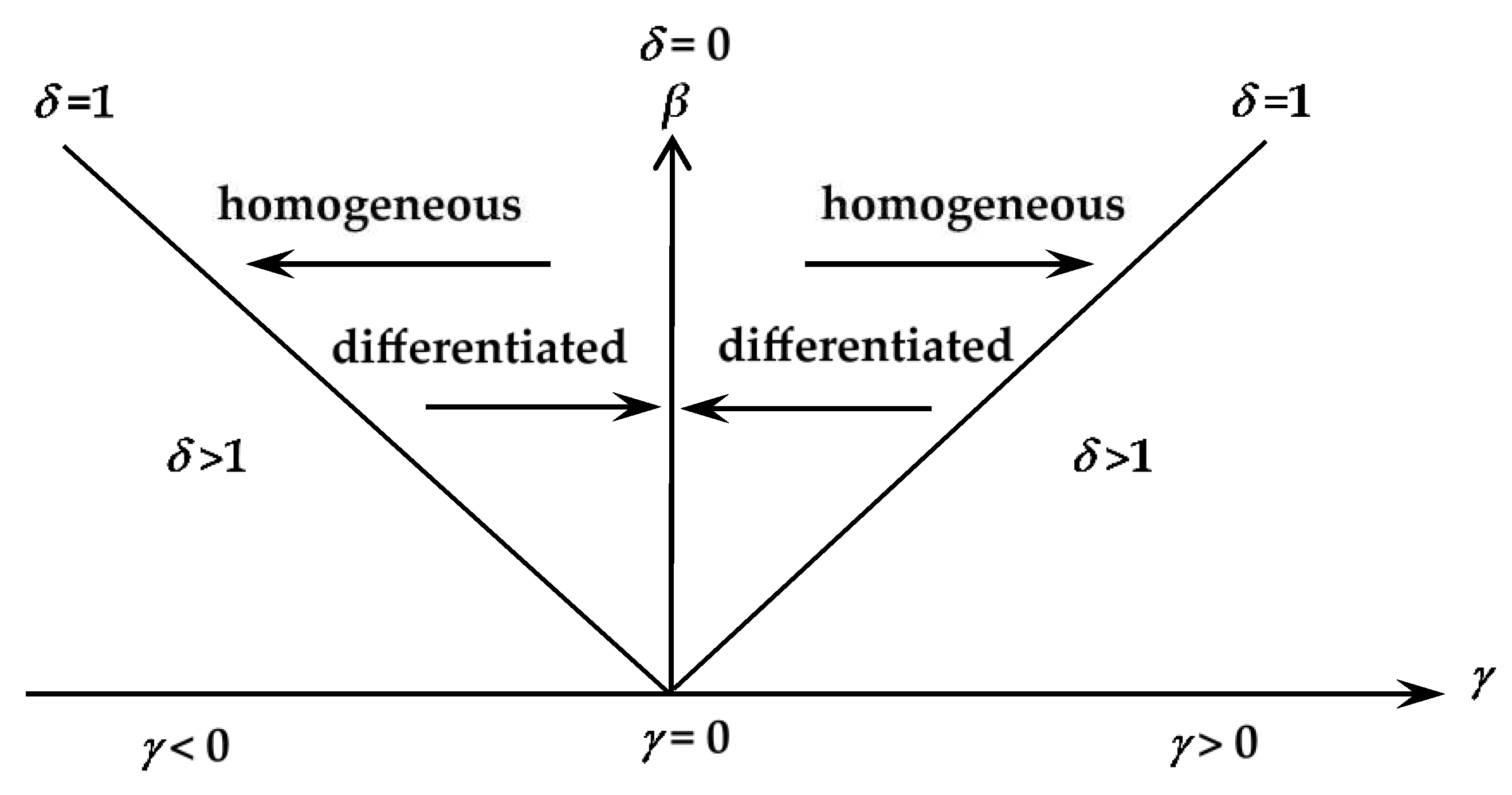
Figure 2. The outflow of customers after price increase. Weak preference for search.

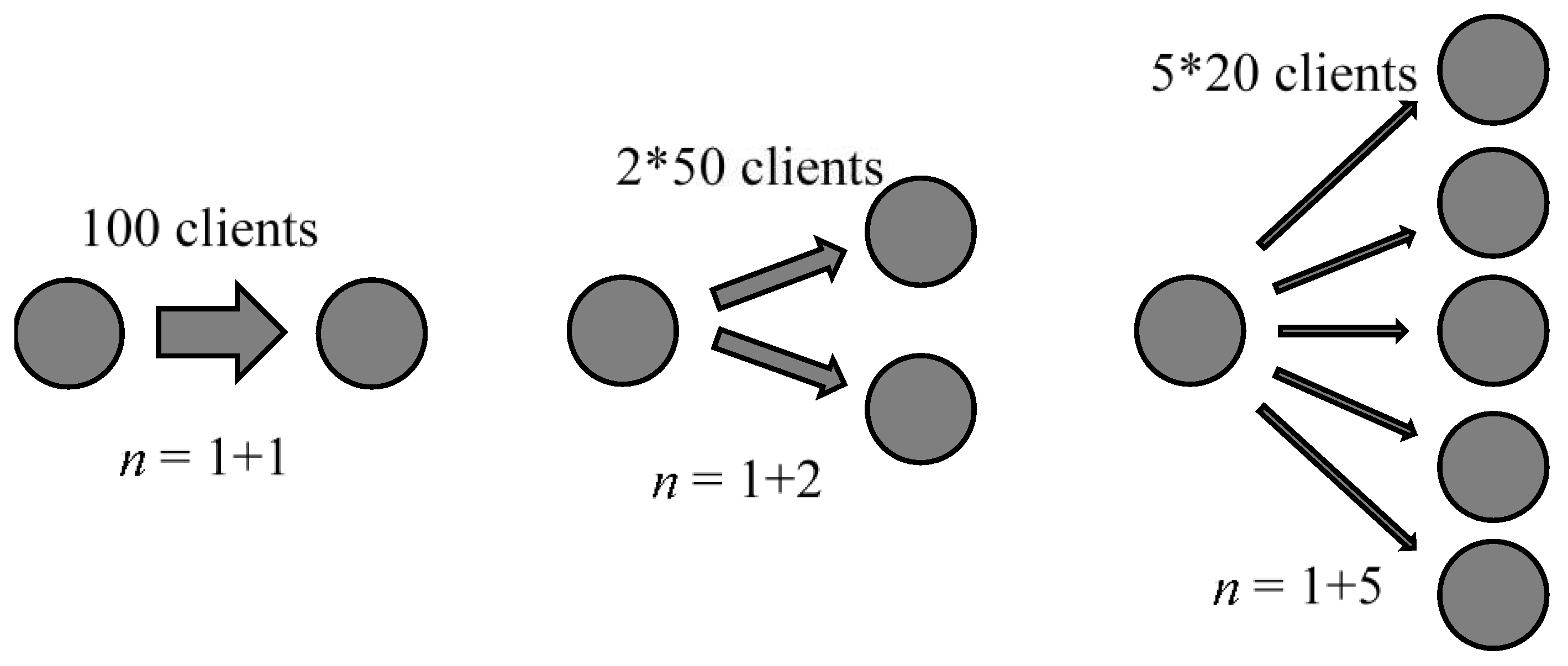
Figure 3. The outflow of customers after price increase. Strong preference for search.

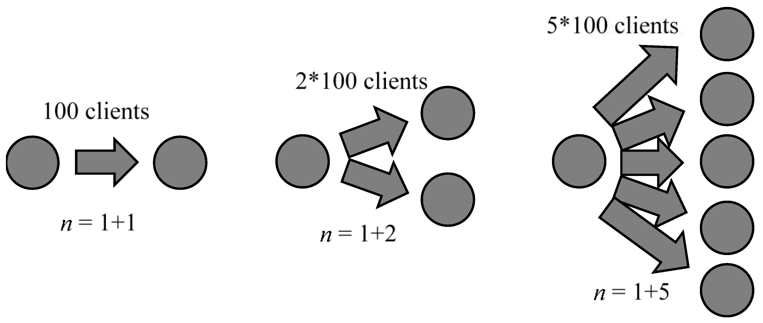
Figure 4. Dependence of the total price of the product on the nominal price, the customer’s location and transportation costs.

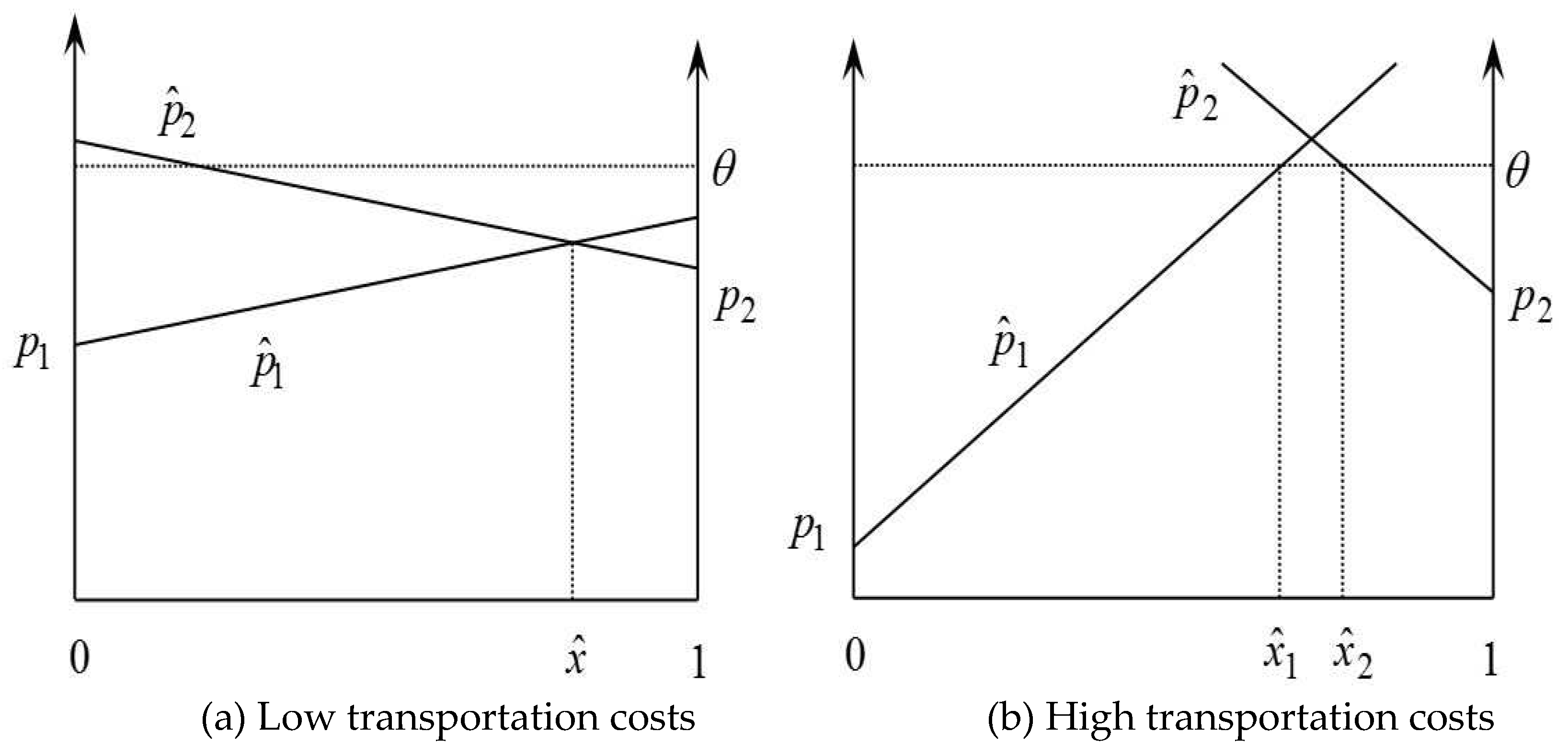
Figure 5. Distribution of buyers between stores in a two-dimensional model.

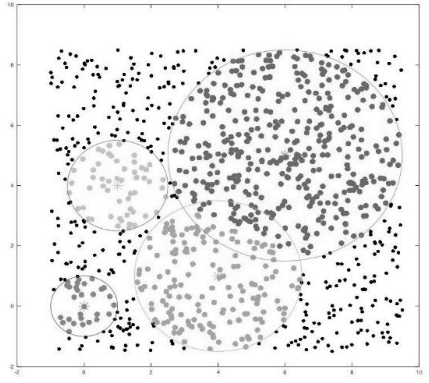
Figure 6. The inversion in situation of high prices

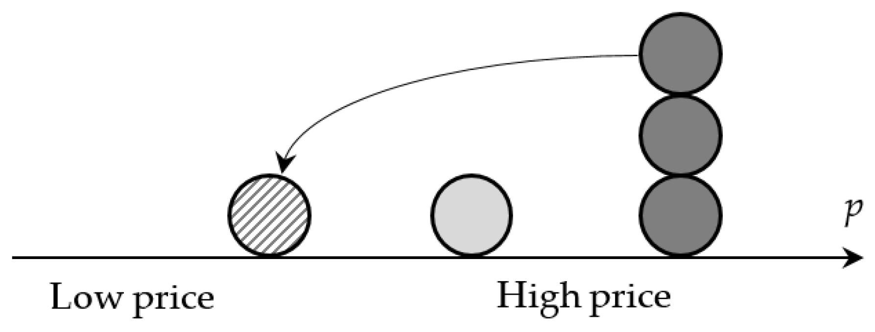
Figure 7. The inversion in situation of low prices

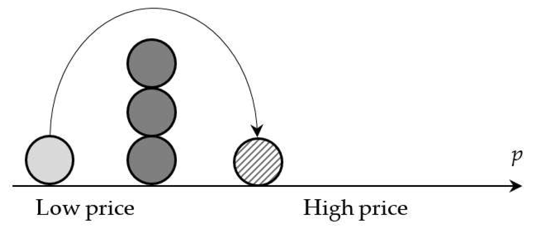
Table 1. Dependence of demand q₁ on prices p₁ and p₂

p₁ / p₂	60	70	80	90	100	110	120	130	140	150
60	3125	4703	5324	5747	5835
70		2742	4147	4740	5038	5184
80			2473	3708	4131	4353	4482
90				2130	3194	3527	3763	3836
100					1807	2651	2940	3076	3153
110						1452	2121	2335	2545	2471
120							1131	1636	1770	1877
130								802	1131	1236
140									474	619
150										187

Table 2. Dependence of demand q₂ on prices p₁ and p₂

p₁ / p₂	60	70	80	90	100	110	120	130	140	150
60	3089	1305	594	236	41
70		2775	1185	479	166	36
80			2477	1017	441	155	32
90				2087	829	350	108	23
100					1788	722	253	79	9
110						1446	546	190	42	5
120							1100	362	115	32
130								852	227	44
140									441	84
150										164

Table 3. Dependence of the total demand Q=q₁+q₂ on prices p₁ and p₂

p₁ / p₂	60	70	80	90	100	110	120	130	140	150
60	6214	6008	5918	5983	5876
70		5517	5332	5219	5204	5220
80			4950	4725	4572	4508	4514
90				4217	4023	3877	3871	3859
100					3595	3373	3193	3155	3162
110						2898	2667	2525	2587	2476
120							2231	1998	1885	1909
130								1654	1358	1280
140									915	703
150										351

Table 4. Economic indicators of firms. The basic model. Weak preference for search, Δ=1

n	2	3	4	5	6	7	8	9	10
Δ	1	1	1	1	1	1	1	1	1
p₁	80,0	73,9	69,7	66,8	64,6	62,9	61,5	60,4	59,5
p*	85,0	77,1	71,9	68,3	65,7	63,7	62,2	61,0	60,0
q₁	45,0	31,9	24,7	20,1	17,0	14,7	13,0	11,6	10,5
q*	35,0	27,1	21,9	18,3	15,7	13,7	12,2	11,0	10,0
π₁	1350	762	487	338	248	190	150	121	100
π*	1225	734	478	334	246	189	149	121	100
π	2575	2231	1921	1673	1478	1321	1194	1088	999

Table 5. Economic indicators of firms. The basic model. Medium preference for search, Δ=2(n–1)/n.

n	2	3	4	5	6	7	8	9	10
Δ	1	1,33	1,5	1,6	1,67	1,71	1,75	1,78	1,8
p₁	80,0	69,6	64,5	61,5	59,5	58,1	57,1	56,3	55,6
p*	85,0	71,6	65,6	62,2	60,0	58,4	57,3	56,5	55,8
q₁	45,0	32,7	25,4	20,7	17,5	15,1	13,3	11,9	10,7
q*	35,0	28,8	23,3	19,4	16,6	14,5	12,8	11,5	10,4
π₁	1350	643	369	239	166	123	94	74	60
π*	1225	622	363	236	165	122	94	74	60
π	2575	1888	1460	1183	993	855	750	668	602

Table 6. Economic indicators of firms. The basic model. Strong preference for search, Δ=n–1.

n	2	3	4	5	6	7	8	9	10
Δ	1	2	3	4	5	6	7	8	9
p₁	80,0	64,5	58,1	55,1	53,5	52,5	51,9	51,5	51,2
p*	85,0	65,4	58,4	55,2	53,5	52,6	51,9	51,5	51,2
q₁	45,0	33,8	26,3	21,4	18,0	15,5	13,6	12,1	10,9
q*	35,0	30,9	25,2	20,9	17,7	15,3	13,5	12,0	10,9
π₁	1350	489	214	109	63	39	26	18	13
π*	1225	477	211	109	63	39	26	18	13
π	2575	1442	848	545	376	274	208	163	131

Table 7. Economic indicators of firms. The .two-stage model. Weak preference for search, Δ=1.

n	2	3	4	5	6	7	8	9	10
Δ	1	1	1	1	1	1	1	1	1
p₁	81,9	75,0	70,3	67,1	64,8	63,0	61,6	60,5	59,6
p*	85,5	77,2	71,9	68,3	65,7	63,7	62,2	61,0	60,0
q₁	42,6	30,6	24,1	19,8	16,8	14,6	12,9	11,5	10,5
q*	35,5	27,2	21,9	18,3	15,7	13,7	12,2	11,0	10,0
π₁	1360	764	488	338	248	190	150	121	100
π*	1258	741	479	334	246	189	149	121	100
π	2618	2246	1925	1675	1478	1322	1194	1088	999

Table 8. Economic indicators of firms. The two-stage model. Medium preference for search, Δ=2(n–1)/n.

n	2	3	4	5	6	7	8	9	10
Δ	1	1,33	1,5	1,6	1,67	1,71	1,75	1,78	1,8
p₁	81,9	70,5	65,0	61,8	59,7	58,3	57,2	56,4	55,7
p*	85,5	71,8	65,6	62,2	60,0	58,4	57,3	56,5	55,8
q₁	42,6	31,4	24,6	20,2	17,1	14,8	13,1	11,7	10,6
q*	35,5	29,0	23,4	19,5	16,6	14,5	12,8	11,5	10,4
π₁	1360	646	370	239	167	123	94	74	60
π*	1258	631	366	237	166	122	94	74	60
π	2618	1908	1469	1189	996	857	751	669	602

Table 9. Economic indicators of firms The two-stage model. Strong preference for search, Δ=n–1.

n	2	3	4	5	6	7	8	9	10
Δ	1	2	3	4	5	6	7	8	9
p₁	81,9	64,9	58,3	55,2	53,5	52,5	51,9	51,5	51,2
p*	85,5	65,5	58,4	55,2	53,5	52,6	51,9	51,5	51,2
q₁	42,6	32,9	25,9	21,2	17,9	15,5	13,7	12,1	11,2
q*	35,5	31,1	25,3	20,9	17,7	15,3	13,5	12,0	10,8
π₁	1360	491	214	110	63	39	26	18	13
π*	1258	483	213	109	63	39	26	18	13
π	2618	1458	853	546	377	274	208	163	131

Table 10. Economic indicators of firms. The two-stage model with expensive leaders. Weak preference for search, Δ=1.

n	2	3	4	5	6	7	8	9	10
Δ	1	1	1	1	1	1	1	1	1
p₁	81,2	80,4	79,9	79,6	79,3	79,1	78,9	78,8	78,7
p*	88,5	94,5	97,4	99,0	100,1	100,8	101,4	101,8	102,1
q₁	46,8	40,6	37,4	35,5	34,2	33,3	32,6	32,0	31,6
q*	32,1	19,5	14,2	11,2	9,3	7,9	6,9	6,1	5,5
π₁	1457	1236	1121	1050	1002	968	942	922	905
π*	1235	867	673	550	465	403	356	318	288
π	2692	2971	3140	3251	3330	3388	3433	3469	3498

Table 11. Economic indicators of firms. The two-stage model with expensive leaders. Medium preference for search, Δ=2(n–1)/n 1.

n	2	3	4	5	6	7	8	9	10
Δ	1	1,33	1,5	1,6	1,67	1,71	1,75	1,78	1,8
p₁	81,2	76,1	73,9	72,7	71,9	71,4	71	70,7	70,4
p*	88,5	87,8	87,5	87,3	87,2	87,1	87,1	87,0	87,0
q₁	46,8	43,5	41,9	40,9	40,2	39,7	39,3	39,0	38,8
q*	32,1	20,2	14,7	11,6	9,6	8,2	7,1	6,3	5,6
π₁	1457	1138	1002	927	880	848	824	806	792
π*	1235	763	552	433	357	303	263	233	209
π	2692	2663	2659	2661	2663	2665	2667	2669	2671

Table 12. Economic indicators of firms. The two-stage model with expensive leaders. Strong preference for search, Δ=n–1.

n	2	3	4	5	6	7	8	9	10
Δ	1	2	3	4	5	6	7	8	9
p₁	81,2	70,4	65,1	61,9	59,8	58,3	57,3	56,4	55,7
p*	88,5	79,3	73,5	69,5	66,6	64,5	62,8	61,5	60,4
q₁	46,8	47,7	48,9	49,9	50,7	51,2	51,7	52,0	52,3
q*	32,1	21,0	15,3	12,0	9,9	8,4	7,3	6,4	5,8
π₁	1457	974	737	593	497	427	375	334	301
π*	1235	615	360	234	164	122	93	74	60
π	2692	2203	1816	1531	1319	1156	1028	925	841

Table 13. Economic indicators of firms according to their number. Cartel.

n	2	3	4	5	6	7	8	9	10
q_i	27,5	18,3	13,8	11	9,2	7,9	6,9	6,1	5,5
π_i	1513	1008	756	605	504	432	378	336	303

Table 14. Economic indicators of firms. The price discrimination model. Weak preference for search, Δ=1.

n	2	3	4	5	6	7	8	9	10
Δ	1	1	1	1	1	1	1	1	1
p₁	101,3	98,1	96,0	94,5	93,4	92,6	92,0	91,5	91,0
p*	116,0	118,8	120,0	120,7	121,2	121,5	121,7	121,9	122,1
q₁	44,0	41,3	40,0	39,3	38,8	38,5	38,3	38,1	37,9
q*	14,7	10,3	8,0	6,5	5,5	4,8	4,3	3,8	3,4
π₁	2259	1985	1840	1749	1687	1641	1606	1579	1556
π*	968	709	560	463	395	344	305	274	249
π	3227	3403	3520	3601	3661	3706	3741	3770	3793

Table 15. Economic indicators of firms. The price discrimination model. Medium preference for search, Δ=2(n–1)/n 1.

N	2	3	4	5	6	7	8	9	10
Δ	1	1,33	1,5	1,6	1,67	1,71	1,75	1,78	1,8
p₁	101,3	100,0	99,3	98,9	98,6	98,4	98,2	98,1	98,0
p*	116,0	115,0	114,5	114,2	114,0	113,8	113,7	113,6	113,5
q₁	44,0	40,0	37,9	36,7	35,8	35,2	34,7	34,4	34,1
q*	14,7	10,0	7,6	6,1	5,1	4,4	3,9	3,4	3,1
π₁	2259	2000	1870	1793	1741	1704	1676	1654	1637
π*	968	650	489	392	327	281	246	219	197
π	3227	3300	3338	3361	3377	3388	3396	3403	3408

Table 16. Economic indicators of firms. The price discrimination model. Strong preference for search, Δ=n–1.

N	2	3	4	5	6	7	8	9	10
Δ	1	2	3	4	5	6	7	8	9
p₁	101,3	101,8	102,3	102,7	103,0	103,3	103,5	103,6	103,7
p*	116,0	111,5	109,5	108,4	107,8	107,3	107,0	106,7	106,5
q₁	44,0	38,8	36,1	34,4	33,2	32,4	31,8	31,3	30,9
q*	14,7	9,7	7,2	5,7	4,7	4,1	3,5	3,1	2,8
π₁	2259	2010	1886	1812	1762	1727	1700	1679	1663
π*	968	597	429	335	274	232	201	178	159
π	3227	3203	3174	3151	3134	3121	3110	3102	3095

Disclaimer/Publisher’s Note: The statements, opinions and data contained in all publications are solely those of the individual author(s) and contributor(s) and not of MDPI and/or the editor(s). MDPI and/or the editor(s) disclaim responsibility for any injury to people or property resulting from any ideas, methods, instructions or products referred to in the content.

© 2023 by the authors. Licensee MDPI, Basel, Switzerland. This article is an open access article distributed under the terms and conditions of the Creative Commons Attribution (CC BY) license (http://creativecommons.org/licenses/by/4.0/).

Copyright: This open access article is published under a Creative Commons CC BY 4.0 license, which permit the free download, distribution, and reuse, provided that the author and preprint are cited in any reuse.

MDPI Initiatives

Important Links

Choose an area of interest and we will send you notifications of new preprints at your preferred frequency.

Disclaimer

Price oligopoly with differentiated product and dependence of total demand on the bottom price

Abstract

1. Introduction

2. The Model

3. Microeconomic Substantiation

4. The Equilibrium

5. The Inversion

6. The Two-Stage Model

7. Cartel and Price Discrimination

8. Discussion

Funding

References

MDPI Initiatives

Important Links

Subscribe