Submitted:
06 October 2023
Posted:
09 October 2023
You are already at the latest version
Abstract
A closed chain of oscillators can be considered as a model of ring-shaped ecosystems, such as atolls or coastal zones of inland reservoirs. As an oscillator model, we use the logistic map that often referred to as an archetypical example of how complex dynamics can arise from very simple nonlinear equations. We investigate the influence of the model parameters both on the nature of oscillations in the oscillator ring and on the spatial structures that arise in this case. Namely, we demonstrate a variety of emerging spatial structures depending on the initial conditions.
Keywords:
coupled chaotic oscillators
; spatial-temporal patterns
; regular patterns
Introduction
Mathematical models have shown high efficiency in studies of qualitative regularities in the functioning of complex systems. One of the significant advantages of this approach is the opportunity to study individual processes separately. For example, the logistic map describing the population dynamics in the absence of external influences depends on only one parameter, the Malthusian coefficient r, the value of which unambiguously determines the dynamical regime of the model (Figure 1). With such a simple model, it was possible to demonstrate the full range of population dynamics: stationary state, periodic oscillations, non-periodic oscillations, and chaotic dynamics [1].
It should be noted that the dynamics of real, not model populations are characterized not only by changes in their properties (abundance, biomass, growth rate) in time, but also, in general, by variations of these properties in space. Only by using spatially distributed models it is possible to study the spatiotemporal dynamics of populations resulting from interspecific competition, migration, and trophic interactions, as well as to form a strategy for sustainable functioning of the population under study [2,3,4,5,6,7]. Simple models with a small number of parameters have been widely used to study phenomena related to spatial dimension of population processes [20}. As such a model, a chain of oscillators can be used, the dynamics of each of which are described both by a logistic map x and by exchange processes between coupled oscillators (see, e.g., [6,7,8]). Such a spatially distributed model allows for a large number of spatial structures and associated effects [7,9,10,11]. Recently, a number of studies describing the behavior of this class of models at different types of coupling (different depth of coupling, coupling with delay) have been conducted [12,13,14], and an attempt has been made to find universal regularities in the occurrence of spatial effects in a chain of diffusively coupled logistic oscillators [15]. Despite the abundance of various effects obtained in these models, no comparison of temporal dynamics and spatial structures has yet been made in a wide range of parameters.
In this work, we set and solved the problem of studying spatiotemporal processes in a closed chain of locally coupled logistic oscillators in a wide range of model parameters (see Model (1) – (2) in Methods). The local coupling between neighboring oscillators of the closed chain can be considered as a model of exchange population processes in ring-shaped ecosystems, such as, for example, the littoral area of an enclosed body of water: a lake or a pond.
.
Results
As a result of numerical experiments covering the range of parameters of Model (1) – (2) (numerical values of r are in the range from 3 to 4, those of parameter D are in the range from 0.001 to 0.5, and those of parameter L are in the range from 2 to 200), all those dynamical regimes characteristic of the pointwise logistic model with discrete time were obtained (Figure 1). In particular, both regular oscillations with different periods and chaotic oscillations were observed (Figure 2, right column, which shows the time series characterizing the dynamics of one of the oscillators in the chain (l = 1), namely, during the last twenty time steps before the end of the numerical experiment; periodic oscillations with period 2 (Figure 2a,b), periodic oscillations with period 4 (Figure 2c,d), and chaotic oscillations (Figure 2e)) can be seen. The middle column (Figure 2) displays the 150 last values of x for each oscillator in the chain. It can be seen that the increase in numerical values of the parameters r and D can lead to a transition from regular to chaotic dynamics in each oscillator in the chain. The left column of Figure 2 shows examples of “spatial” structures demonstrating the distributions of numerical values of x in the chain of oscillators in a particular moment of time. It can be seen from Figure 2 that the transition from regular to chaotic dynamics is accompanied by a significant change in the “spatial” structure. In particular, such a transition results in an increase in the number of peaks with different amplitudes, irregularly distributed along the chain of oscillators.
One of the features of the distributed model (1) – (2) (see also [7]) is its sensitivity to initial conditions for the whole range of values of the parameter r; i.e., both for regular and chaotic oscillators (Figure 2). In the case of an isolated oscillator (when D = 0), the sensitivity to initial conditions is a distinctive feature of the chaotic regime. Since in our case the dependence on initial conditions at D ≠ 0 was not related to regularity or irregularity of both the dynamics of individual oscillators and the nature of “spatial” structures; i.e., the distributions of x values along the chain of oscillators at the selected moment of time t, we used entropy to characterize the spatiotemporal regimes of oscillations in the whole chain as an integral system. The numerical value of entropy at different initial conditions makes it possible to characterize both the dynamics of the system of oscillators and its accompanying spatial structures (examples are shown in Figure 2) depending on their orderliness: a smaller value of entropy corresponds to regular dynamics and relatively more ordered “spatial” structures.
In order to reveal the influence of changes in numerical values of the parameters of Model (1) – (2) on the entropy value, we estimated this value at different numerical values of the parameters r, D, and L. To assess the dynamics of Model (1) – (2), we calculated the “temporal entropy” ET (see Methods), which under given initial conditions characterizes oscillatory processes in a chain of oscillators considered as an integral system. Figure 3 shows the dependence of the probability of low-entropy dynamics, ET < 0.3, on the model parameters under initial conditions that were set randomly. It can be seen that for small values of the chain length (Figure 3, L=2 and L=5), the behavior of the model qualitatively resembles that of the pointwise (at D = 0) logistic map. In particular, this behavior depends significantly on the value of the parameter r. For example, for r values in the range of 3 – 3.5, the dynamics of the model is regular; i.e., low-entropy, with ET < 0.3 at any values of the parameter D. With increasing r, the dynamics becomes irregular, highly entropic, and the probability of low numerical values of ET is close to zero (Figure 3). The narrow vertical regions of low-entropy dynamics at L=2 and L=5 (Figure 3) resemble the windows of regularity in the pointwise logistic map (cf. Figure 1). A significant difference from the pointwise map is the presence of regions with regular dynamics in a wide range of high values of r (Figure 3, regions indicated in yellow at r > 3.6). The presence of such regions indicates that for any r in Model (1) – (2) at relatively small values of the parameter L there will be such a value of the parameter D at which the dynamics of the model is low-entropy. In the space of parameters (r, D), note also the enlargement of such regions that correspond to intermediate (between 0 and 1) values of the probability of observing low-entropy regimes as the length of the oscillator chain increases (in Fig.3, these regions are marked with colors other than yellow and dark blue). At L = 2 and L = 5 such regions are hardly noticeable, but with increasing L their area increases distinctively. This means that the dynamics of the oscillator chain at r > 3.6 depends more and more noticeably on the initial conditions with increasing chain length. At the same time, at r ≤ 3.5, the increase in L does not affect the regime of the dynamics of the oscillator chain; the dynamics remains low-entropy (Figure 3).
To assess the degree of orderliness of the spatial structures (some examples of these structures are given in the left column in Figure 2), we determined such a value of “spatial entropy” Ex (see Methods) that was established by the time the numerical experiment ended. The dependence of Ex on the parameters of Model (1) – (2) is shown in Figure 4.
Figure 4 shows the values of spatial entropy (see Methods), using which we estimated the regularity of “spatial” structures at the end of the computations. Given that for many values of the parameters r and D, the final shape of spatial distribution of x depends on the initial conditions, we computed the space average for 100 initial values. To avoid subtraction of “spatial” structures in antiphase, the x values of each chain were shifted so that the minimum value was in the first oscillator. Thus, regular structures are preserved under averaging and correspond to low spatial entropy. High entropy (yellow and light green colors; Figure 4) are characteristic of highly irregular structures. Dark blue regions are typical of regular structures, such as those in Figure 2d and Figure 6. In other cases, the emergent structures are irregular. It should be noted that in some regions of the r and D parameters space the solution reduces to the pointwise map: the x values in all oscillators are the same, the exchange between oscillators is absent, and the dynamics in each oscillator is similar to that of the pointwise map at the same r value. The areas of r and D values for such cases are shown in white in Figure 4.
If we compare the regions with regular dynamics at r>3.6, demonstrated in Figure 3, and the regular structures in the same regions (Figure 4), we find that these areas overlap to a large extent. Having plotted the average values of (for 100 experiments with different initial conditions) at the last step of the computations in all oscillators in the chain for a fixed value of r, we obtained the picture presented in Figure 5. It can be seen that clear periodic structures are characteristic of many model parameter values. The period of such structures increases with increasing value of the parameter D.
in each oscillator at time t (see Methods) for different initial conditions depending on the value of the parameter D; r=3.808. a) L = 20, b) L = 100, c) L = 200.
It should also be noted (Figure 5) that the length of the oscillator chain L affects the formation of such structures. With increasing length of the oscillator chain, the structures become less clear, and the range of values of the parameter D, in which regular structures are observed, decreases.
Figure 6 shows the examples of distribution of values in the oscillators of the chain at different random initial values, for different chain lengths (left and middle column), and the mean value of for each oscillator in the chain for 100 initial values with the same chain lengths (right column). It can be seen that the examples of the distribution of the values of x in the oscillators of the chain given in Figure 6 are similar, consisting of periodically repeating structures similar in shape but differing in amplitude. The distribution of mean values of x in each oscillator of the chain, using which it is possible to characterize the spatial distribution of x for selected model parameters (r and D) for different initial values, depends qualitatively on the chain length L. In the case when the period of the repeating “spatial” structures is a divisible of the chain length, we can see regularly repeating spatial structures of average values of with the shapes close in amplitude (Figure 6a, 10 peaks; Figure 6c, 11 peaks), otherwise such regularity is significantly disrupted (Figure 6b).
in each oscillator of the chain for two different initial conditions (left and middle columns) and the average values of for each oscillator in the chain for 100 different initial values (right column). r = 3.8; D = 0.32; a) L = 90, b) L = 93, c) L = 95.
Discussion and Conclusion
The logistic map is one of the simplest mathematical models of population dynamics. Although its use for the numerical description of specific biological populations is significantly limited, studies of the logistic map made it possible to reproduce and investigate those dynamical regimes that are characteristic of natural populations. The simplest model that was used in an attempt to account for the spatial heterogeneity of ecological systems is a model system including two coupled logistic oscillators [7,16,17,18,19]. As a result of research on such models, the effects related to synchronization/desynchronization of oscillations of coupled oscillators as well as the effects related to imposing the dynamics of one oscillator on the dynamic mode of the whole system were described.
An even greater variety of both spatial structures and dynamical regimes was obtained from studies of chains of globally coupled oscillators [12,13,14,15]. The main problem with this approach is that a large number of both parameters and ways of setting global couplings arise in such models, making it difficult to identify general patterns for systems of this kind.
In our work, we studied a chain of locally coupled logistic oscillators. We have shown that when the chain length is short (Figure 3), the dependence of the model dynamics on the parameter r is similar to that typical of the pointwise model. As the chain length increases, this correspondence gets broken in the range of high values of the parameter r. In particular, as the chain length increases, the space of the parameters r and D increases as well, for which the dynamics of the model depend on the initial conditions (Figure 3, colors other than yellow and dark blue). It should be noted that the transition boundary between low-entropy (regular) and high-entropy (irregular) dynamics remains unchanged when the chain length is changed (Figure 3).
The “spatial” structures arising as a result of regular oscillations in a chain of oscillators have an arbitrary shape in a wide space of the parameters r and D. The shape of such structures is irregular and depends significantly on initial conditions. Only in the range of the values of the parameter r>3.6 there is a region with regular dynamics, for which the shape of spatial structures demonstrates periodicity (Figs 5, 6). It should be noted that this range also demonstrates the dependence of spatial structures on initial conditions; however, their periodicity remains unchanged. Figure 7 shows the “spatial” structures arising under different initial conditions (first and second columns) and the spatial structures averaged over 100 randomly set initial conditions (third column) for high-entropy dynamics (Figure 7a,b), for low-entropy dynamics with resulting disordered spatial structures (Figure 7c,d) and for low-entropy dynamics with resulting spatial structures characterized by a periodic arrangement of peaks (Figure 7e). Although the amplitude of the peaks in such structures (Figure 7e) depends on initial conditions, their periodicity is preserved, which is clearly expressed for the averaged values (Figure 7, third column). At the same time, the averages presented in Figure 7a–d (third column) demonstrate neither a distinct shape, nor periodicity and are similar to each other, despite resulting from both high-entropy and low-entropy oscillations.
In [11], we described the mechanism of transformation of chaotic dynamics into a regular one due to the resonance of natural vibrations of oscillators and vibrations characteristic of exchange processes between neighboring oscillators.
over 100 random initial conditions (third column) L = 100; a) r = 3.65, D = 0.01, b) r = 3.65, D = 0.05, c) r = 3.4, D = 0.01, d) r = 3.4, D = 0.05, e) r = 3.808, D = 0.33.
The results of this study allowed us to clarify this mechanism. Such resonance occurs only if the period of the spatial structures arising in such a process is a multiple of the chain length or very close to it. The probability of occurrence of such a resonance decreases with the increasing length of the chain of coupled oscillators (Figure 5, areas with no clear alternation of yellow and blue bands increase with increasing chain length).
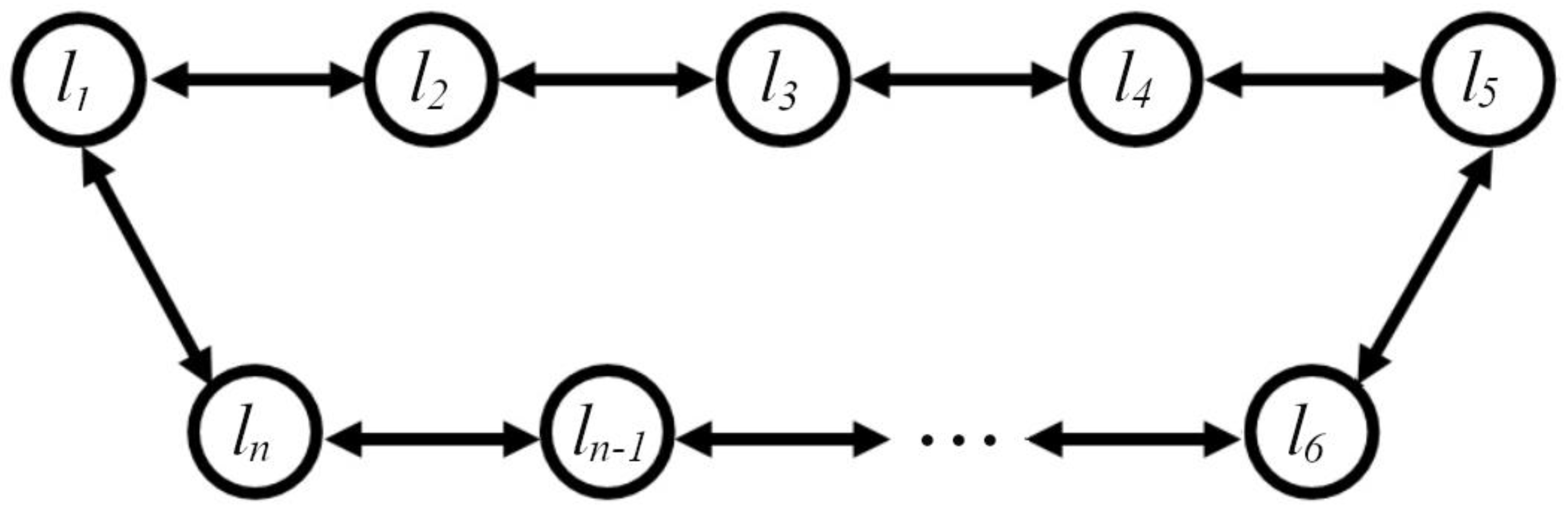
Logistic maps (2) have been widely used in mathematical modeling of ecological processes [20,21]. Mathematical Model (1) – (2) presented here couples the oscillators, the dynamics of which are described by the logistic map, into a closed chain (Figure 9). The characteristics of oscillatory processes in such a chain, as shown in this work, depend both on the intrinsic dynamics of the oscillators included in the chain and the exchange processes between neighboring oscillators, as well as, in general, on the number of oscillators in the chain.
The chain of closed oscillators can be seen as a reduced description of natural ring-shaped ecosystems, such as atolls or littoral areas of enclosed bodies of water (lakes, ponds). In this work, we limited ourselves to a model of spatial heterogeneity and its role in the formation of holistic characteristics; i.e., the spatiotemporal characteristics of the ring-shaped ecosystem as a whole. Spatial heterogeneity of coastal ecosystems (e.g., in marine ecosystems in the vicinity of atolls) depends on a plethora of biotic and abiotic factors [22]. In particular, this heterogeneity may be a consequence of the spatial distribution of sea currents that transport organic matter to atoll shores. In addition, a source of spatial heterogeneity of ecosystems in the vicinity of atolls is the transfer of biogens from the coast to the ocean. In this case, the source of biogens is the excrement of fish-eating birds that return from upwelling areas to their nesting sites on the shore of the atoll [23]. Enrichment of coastal waters with biogenic elements (guanotrophication) is also provided by colonial hydrophilic birds that nest on lake shores [24,25]. Spatial heterogeneity in coastal ecosystems of enclosed water bodies can also be caused by anthropogenic impacts on such ecosystems [26,27].
In Model (1) – (2), heterogeneity of the oscillator dynamics within the chain is set not by the intrinsic properties of the oscillators themselves, which are assumed to be identical, but by different initial conditions. Different initial conditions of the model oscillators can be matched with very different mechanisms underlying the heterogeneity of natural ecosystems. In addition, unlike time t, the spatial length of the chain of the model oscillators is not defined in any way. Therefore, we can assume that the dynamical regimes and spatial structures that result from oscillator interactions (Figs. 2 – 7) can be reproduced in real ring-shaped ecosystems at different spatial scales. The results presented in this paper are aimed particularly at identifying such indicators that characterize key features of the functioning of ring-shaped ecosystems.
Methods
In this work, we studied a chain of locally coupled logistic oscillators, the structure of which is shown in Figure 8.
Logistic equation as a map of a nonlinear operator
The logistic equation can be written as a map of a vector to a vector by means of a nonlinear operator
The nonlinear operator acting on the vector is defined as follows:
The notation ○ in the formula stands for the Hadamard product (also known as the elementwise product, entrywise product, or Schur product) and is a binary operation that takes two matrices of equal dimensions and returns a matrix of the multiplied corresponding elements.
The symbol denotes matrix multiplication, where the matrix is a circulant matrix of dimension , each row of which contains exactly three non-zero elements. Each subsequent row of the matrix is obtained by cyclically shifting the elements of the previous row to the right:
Here is the length of the chain of coupled logistic oscillators, is the exchange value between neighboring oscillators, is the Malthusian coefficient of the logistic map . The parameters of the logistic equation enter only the matrix .
The logistic map at given parameters and under given initial conditions can be considered as a method of simple iteration of the solution of a nonlinear equation of the form:
In equation (2), P is the degree of the nonlinear operator and X is the solution of equation (2). In the method of simple iterations, we will say that the solution of equation (2) is found if, starting from someN1, the following condition is satisfied:
where . In practice, it is convenient to use the value of the residual difference norm at successive iteration steps to search for a solution simultaneously with the search for the period P:
where N2 is an arbitrary number.
The exact solution of equation (2) with period P is obtained if the following conditions are satisfied:
where P is the index of the first zero of vector zi. Obviously, along with (3), the conditions for all points with period P are satisfied:
For nonlinear equation (2), depending on parameters r, D, many various solutions with different periods can be obtained depending on the initial conditions. In addition to exact solutions with condition (3), there may exist reasonably stable approximate solutions, for which the following inequalities are satisfied:
It is important to note here that conditions (4) must be satisfied simultaneously for all points with period P, since there can be a situation where the fulfillment of (4) for k=1 does not guarantee the fulfillment of condition (4) for k=10. In the process of iterations, modes with close frequencies may be present in the system, which will lead to beats modulating the minima additionally with a rather low frequency equal to the difference of frequencies of the two modes.
For some initial conditions, there can be no solutions in the exact sense of (3) even for relaxed criterion (4). At the same time, we cannot claim that solutions with these initial conditions do not exist because the method of simple iterations has its limitations (it may simply fail to converge to a solution). However, by applying this method to all random initial conditions for a point in the area of parametersrand D, we make the same methodological error, which enables us to draw general conclusions on the existence of exact solutions in the parametric pointr, D.
In order to understand the structure and behavior of solutions in some point of parametersrand D, it is necessary to obtain solutions for a whole set of initial conditions by the method of simple iterations using relaxed criterion (4) for given value . Calculations for each point r, D are performed using the algorithm below.
Algorithm for finding solutions for a set of initial conditions
The general idea of the algorithm is to simultaneously iterate several vectors , while taking out of iterations those for which condition (4) is satisfied. Formally, this is possible by substituting vector with rectangular matrix B of dimension of the form in equation (1).
From the formal point of view, substitution of matrixBfor vector in equation (1) does not result in any computational advantages; however, the use of modern libraries accounting for multicore, multithreading, the presence of computational pipelines and a large amount of cache memory of modern processors, multiplication of discharged matrix A by the full matrix is much more preferable than sequential multiplication ofAby the number of vectors equal to the number of columns in the full matrix.
The algorithm consists of a number of steps, with the help of which, from the initial random matrixB, we obtain a matrix, several (or all) columns of which are solutions, and the other (if any remain) are not solutions. It is important that further iterations over this matrix do not change the picture. Considering the latter, we will refer to the results of the algorithm as generalized solutions. They may include both solutions proper (condition (3)) and approximate solutions with given accuracy ((4)).
A step of the algorithm includes sequential application of some (N1) “blind” iterations, where we care not about the intermediate results but only about matrix , and then some number (N2) of “measuring” iterations, where the set of all intermediate matrices is preserved: .
Having a set of intermediate matrices, we calculate the matrix of residuals according to the following formula:
For set criterion we check condition (4) for all rows of matrixZ. Each row corresponds to one initial condition (column of matrix B). We separate the convergent solutions, write them down separately, and remove them from the matrixB. This reduces the number of its columns.
We proceed to the next step (iteration) of the algorithm, where matrix B reduced at the previous iteration is used as the initial matrix. Exit from the iteration loop occurs either when matrixBbecomes empty (all columns converged to an exact or approximate solution) or when the iterative process stagnates. To check for stagnation, prior to the iterations we pre-fill the auxiliary arrayCZof lengthNCZ, equal to the allowed number of stagnating iterations, with units. At each iterative step of the algorithm we assign to the first element of this array the number of columns for which condition (4) is satisfied, and then we cyclically shift the elements of this array to the right by one step. Then we check the sum of its elements. If the sum is zero, we exit the operations and terminate the algorithm; if not, we continue the iterations. If we exit by stagnation, we simply add the columns that did not converge to the solution to those that we previously separated from matrixBas converging to the solution. Note once again that we refer to all the columns of matrix B obtained at the output of the algorithm as generalized solutions.
Once the computations are complete for all initial conditions, we can estimate the probability of obtaining solution Ps with given accuracy for a point in the parametric spacer, Dfor random initial conditions:
where is the number of columns of matrix B, for which condition (4) is satisfied.
It should be noted that for a given point in the parametric spacer, D, if in the set of generalized solutions there exist solutions for which condition (4) is satisfied, the remaining solutions will be similar in some sense. At a minimum, they will have periodic residuals (5). For the general analysis of the residuals generated by matrix of generalized solutionsB, it is convenient to introduce the relative spectral entropy for all rows of the matrix of residuals (5). Next, we outline the general scheme for calculating spectral entropy and then write out formulas for the relative spectral entropy of the residuals.
Spectral entropy of an arbitrary valid signal
The spectral entropy of the arbitrary signal of the length normalized to the unit of the power spectrum, is an estimate of the entropy by Shannon’s formula. There are many ways to estimate the signal power spectrum, here is the simplest one. A biased signal, the mean of which is not zero, has a singularity at the zero frequency of the spectrum, which will interfere with the analysis. In order to remove the constant component of the signal, we remove the linear trend from it, subtract from the signal the values that were obtained from the linear regression, which is built on the points . Then we perform the Fourier transform of the signal. Let the signal without trend form a columnY, then the sought Fourier image is a linear transform with the Fourier matrixF:
The elements of the Fourier matrix are given by the following expression
The normalized power spectrumS(k)of the valid signal is given by the following expression:
For a valid signal, the square of the modulus of its Fourier image is symmetric about the center, so the informative part of the spectrum lies in the region from 1 to . The spectral entropy of signal after
finding its power spectrum is
calculated using Shannon's formula:
The argument in square brackets emphasizes that the spectral entropy E is a functional of the signal Y.
Relative spectral entropy of residuals (temporal entropy)
To estimate the degree of periodicity of the solutions, it is sufficient to calculate the spectral entropy of the residuals (5). For convenience in comparing values, it makes sense to divide the entropy value by its maximum value, which it takes for a constant power spectrumS=2/n:
The relative spectral entropy of the residuals or temporal entropy in the adopted notations will be written as:
In the case when the signal is periodic in time , if not, is close to 1. Choosing some boundary value of the relative entropy, say 0.3, we can estimate the probability that at a given point in the parametric spacer, Dthe relative temporal entropy will be less than the boundary value. To do this, we need to count the number of cases where and divide it by the total number of trialsM.
Relative spectral entropy of solutions (spatial entropy)
In addition to periodicity of solutions in time (iterations), there may be periodicity of solutions in “space” (periodic variation along sites). In complete analogy to the previous statement, we can estimate the spatial entropy for each solution in the solution matrixB. The only difference from time entropy would be the doubling of the length of the original function, so that entropy estimates can be made for both short chains and chains with an odd number of links. This can be achieved by docking two identical solutions together, thereby doubling the length of the analyzed signal. In this case, the power spectrum will be defined atLpoints. The formula of spatial entropy is as follows:
as for the temporal entropy, we can estimate the probability that at a given point of the parametric spacer, Dthe relative spatial entropy will be less than the boundary value. It is equal to the number of cases when , divided by the number of trialsM.
Mean value of generalized solutions, entropy of the mean solution
An important quantity characterizing the structure formation at the parametric pointr, Dcould be the average over all columns of the matrix of generalized solutions valueB, which we denote as . Direct computation will show us a close to straight line, since all generalized solutions have an arbitrary random phase. However, a feature of (1) with a circulant matrixAis the invariance of the generalized solutions with respect to an arbitrary cyclic shift of the elements of the generalized solutions . We will take advantage of this and before averaging the generalized solutions we perform a cyclic shift so that the minimum value is in the first element of the vector: . In this case, all generalized solutions appear to be in the same phase, and their average will be an informative quantity. An additional numerical characteristic of orderliness can be the spatial entropy:
Funding: The reported study was funded by the Institute of Theoretical and Experimental Biophysics of the Russian Academy of Sciences (state assignment № 075-01025-23-01) and by the Institute of Mathematical Problems of Biology, Keldysh Institute of Applied Mathematics of the Russian Academy of Sciences (state assignment 0017-2019-0009).
References
- May, R.M. Biological populations with non-overlapping generations: Stable points, stable cycles, and chaos. Science 1974, 13, 311–326. [Google Scholar]
- Abta, R.; Schiffer, M.; Ben-Ishay, A.; Shnerb, N.M. Stabilization of metapopulation cycles: Toward a classification scheme. Theoretical Population Biology 2008, 74, 273–282. [Google Scholar] [CrossRef]
- Kerr, B.; Neuhauser, C.; Bohannan, B.J.M.; Dean, A.M. Local migration promotes competitive restraint in a host–pathogen ‘tragedy of the commons’. Nature 2006, 442, 75–78. [Google Scholar] [CrossRef]
- Zion, Y.; Yaari, G.; Shnerb, N. Optimizing Metapopulation Sustainability through a Checkerboard Strategy. Computational Biology January 2010, 6(1), 1–9. [Google Scholar]
- Kulakov, M.; Neverova, G.; Frisman, E. The Ricker Competition Model of Two Species: Dynamic Modes and Phase Multistability, Mathematics 2022, 10(7), 1076. 10.
- Dzwinel, W. Spatially extended populations reproducing logistic map. Cent. Eur. J. Phys. 2010, 8(1), 33–41. [Google Scholar] [CrossRef]
- Lloyd, A. The Coupled Logistic Map. A Simple Model for the Effects of Spatial Heterogeneity on Population Dynamics. J. theor. Biol. 1995, 173, 217–230. [Google Scholar] [CrossRef]
- Kaneko, K. Period-doubling of kink-antikink patterns, quasiperiodicity in antiferro-like structures and spatial intermittency in coupled logistic lattice. Progress of Theoretical Physics 1984, 72(3), 480–486. [Google Scholar] [CrossRef]
- Bruce, E. , Kendall Spatial Structure, Environmental Heterogeneity, and Population Dynamics: Analysis of the Coupled Logistic Map. Theoretical Population Biology 1998, 54, 11–37. [Google Scholar]
- Savi, M. A. Effects of randomness on chaos and order of coupled logistic maps. Physics Letters A 2007, 364(5), 389–395. [Google Scholar] [CrossRef]
- Rusakov, A.V.; Tikhonov, D.A.; Nurieva, N.I.; Medvinsky, A.B. Emergence of Self-Organized Dynamical Domains in a Ring of Coupled Population Oscillators. Mathematics 2021, 9, 601. [Google Scholar] [CrossRef]
- Willeboordse, F.H. Time-Delayed Map extension to n-dimensions. Chaos, Solitons & Fractals 1992, 2 (4), 411-420.
- Ouchi, N.B.; Kaneko, K. Coupled maps with local and global interactions. Chaos 2000, 10(2), 359–365. [Google Scholar] [CrossRef] [PubMed]
- Rajvaidya, B.P.; Deshmukh, A.D.; Gade, P. M.; Sahasrabudhe, G. G. Transition to coarse-grained order in coupled logistic maps: Effect of delay and asymmetry. Chaos, Solitons & Fractals 2020, 139, 110301. [Google Scholar]
- Willeboordse, F. H. Hints for universality in coupled map lattices. PHYSICAL REVIEW E 2002, 65, 026202. [Google Scholar] [CrossRef] [PubMed]
- Cánovas, J.S. The dynamics of coupled logistic maps. Networks and Heterogeneous Media 2023, 18, 275–290. [Google Scholar] [CrossRef]
- Layek, G.C.; Pati, N.C. Organized structures of two bidirectionally coupled logistic maps. Chaos 2019, 10(2), 093104. [Google Scholar] [CrossRef] [PubMed]
- Metzler, W.; Beau, W.; Frees, W.; Ueberla, A. Symmetry and Self-Similarity with Coupled Logistic Maps. Z. Naturforsch 1987, 42a, 310–318. [Google Scholar] [CrossRef]
- Maistrenko, Yu. L.; Maistrenko, V. L.; Popovych, O.; Mosekilde, E. Desynchronization of chaos in coupled logistic maps. Phys. Rev. E 1999, 60, 2817. [Google Scholar] [CrossRef]
- Kot, M. Elements of Mathematical Ecology. Cambridge University, UK, 2001.
- Solé, R.V.; Bascompte, J. Self-Organization in Complex Ecosystems. Princeton University, USA, 2006.
- Levin, S.A. The problem of pattern and scale in ecology. Ecology 1992, 73, 1943–1967. [Google Scholar] [CrossRef]
- Fosberg, F.R. Qualitative description of the coral atoll ecosystem. Atoll Research Bulletin 1961, 81, 1–11. [Google Scholar] [CrossRef]
- Leentvaar, P. Observations in guanotrophic environments. Hydrobiologia 1967, 29, 441–489. [Google Scholar] [CrossRef]
- Moss, B.; Leah, R.T. Changes in the ecosystem of a guanotrophic and brackish shallow lake in eastern England: potential problems in its restoration. Internationale Revue der gesamten Hydrobiologie und Hydrographie 1982, 67, 625–659. [Google Scholar]
- Ostrovsky, I.; Rimmer, A.; Yacobi, Y.Z.; Nishri, A.; Sukenik, A.; Hadas, A.; Zohary, T. Long-term changes in the Lake Kinneret ecosystem: The effects of climate change and antropogenic factors. In Climate Change and Global Warming in Inland Waters: Impacts and mitigation for Ecosystems and Societies; Robarts, R.D., Goldman, C.R., Kumagai, M., Eds.; Oxford, Wiley & Sons, UK, 2013, 271-293.
- Adamovich, B.V.; Medvinsky, A.B.; Nikitina, L.V.; Radchikova, N.P.; Mikheyeva, T.M.; Kovalevskaya, R.Z.; Veres, Y.K.; Chakraborty, A.; Rusakov, A.V.; Nurieva, N.I.; Zhukova, T.V. Relations between variations in the lake bacterioplankton abundance and the lake trophic state: Evidence from the 20-year monitoring. Ecological Indicators 2019, 97, 120–129. [Google Scholar] [CrossRef]
Figure 1.
Bifurcation diagram of the logistic map: x.
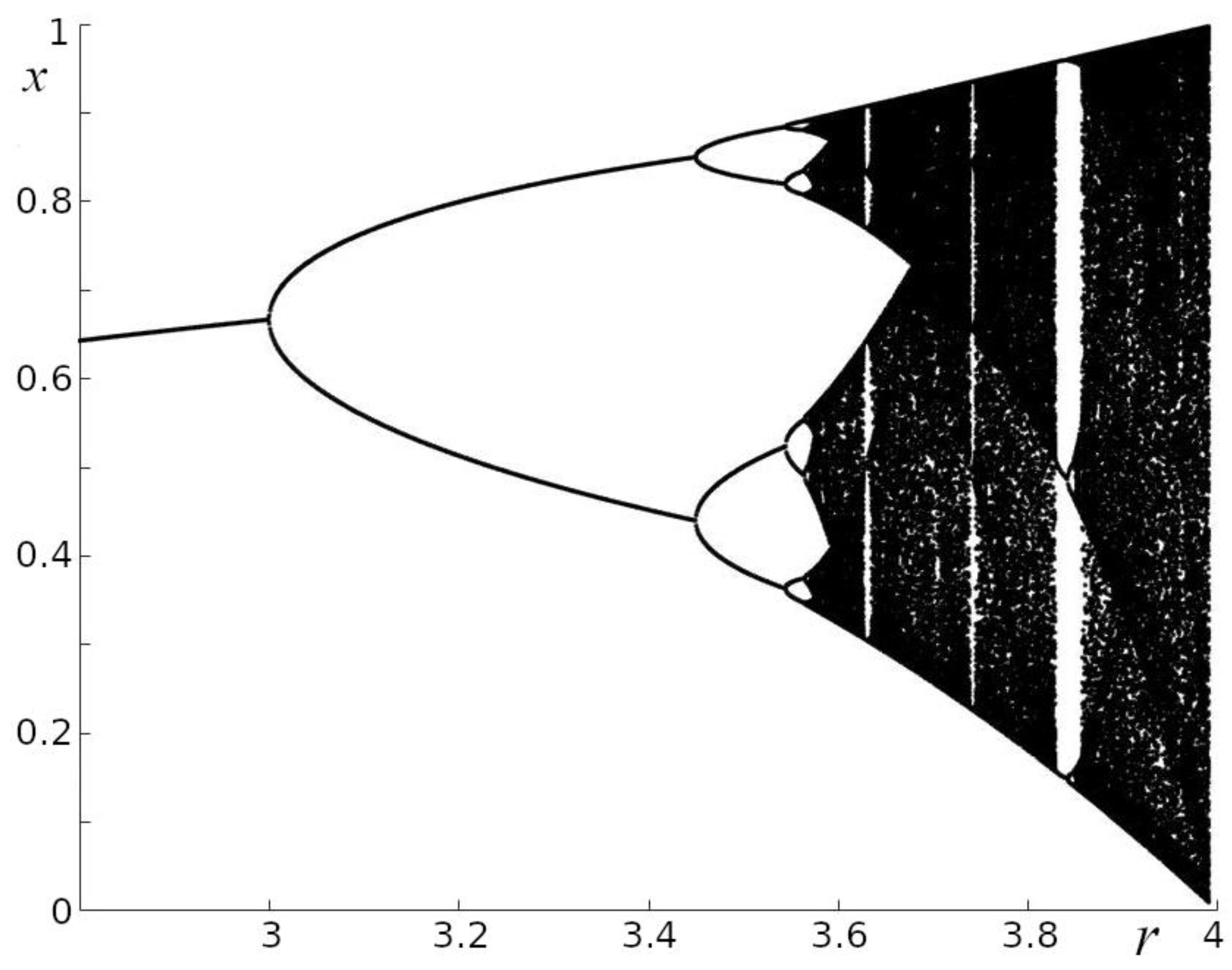
Figure 2.
Examples of spatial and temporal structures for different parameter values of Model (1) – (2) for L = 100. The left column demonstrates the values of Model (1)-(2) in each oscillator at the end of the numerical experiment (see Methods); the middle column shows the 150 last values in each oscillator, and the right column shows the 20 last values in the first (I = 1) oscillator. a, b) r=3.141, D = 0.16 (for different initial conditions); с) r=3.545, D = 0.16; d) r=3.808, D = 0.32; e) r=3.909, D = 0.02.
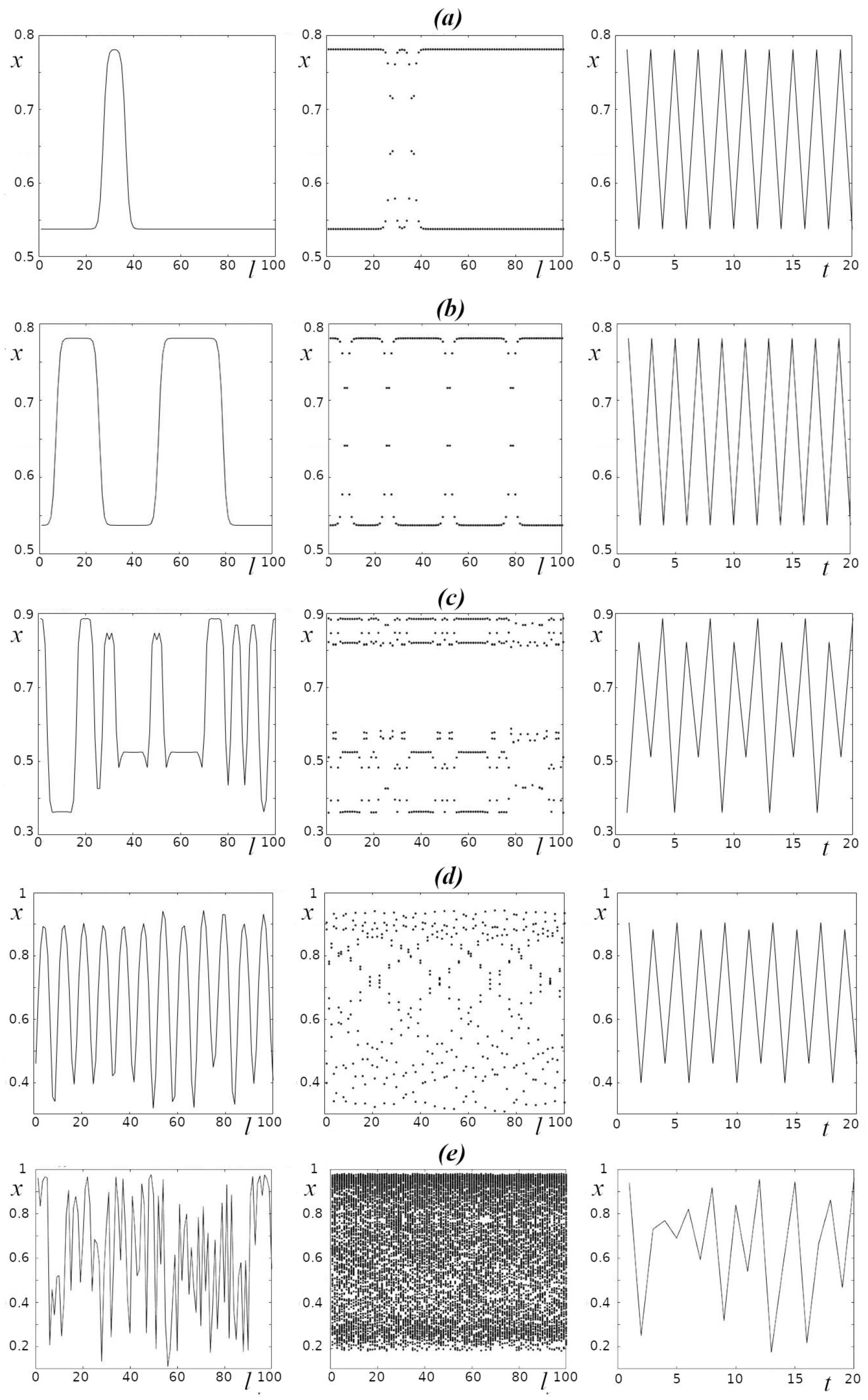
Figure 3.
Probability of observing low temporal entropy (Et <0.3 equation (4)) for different chain lengths L of Model (1) under different initial conditions (100 numerical experiments for each pair of parameters r and D).
Figure 3.
Probability of observing low temporal entropy (Et <0.3 equation (4)) for different chain lengths L of Model (1) under different initial conditions (100 numerical experiments for each pair of parameters r and D).
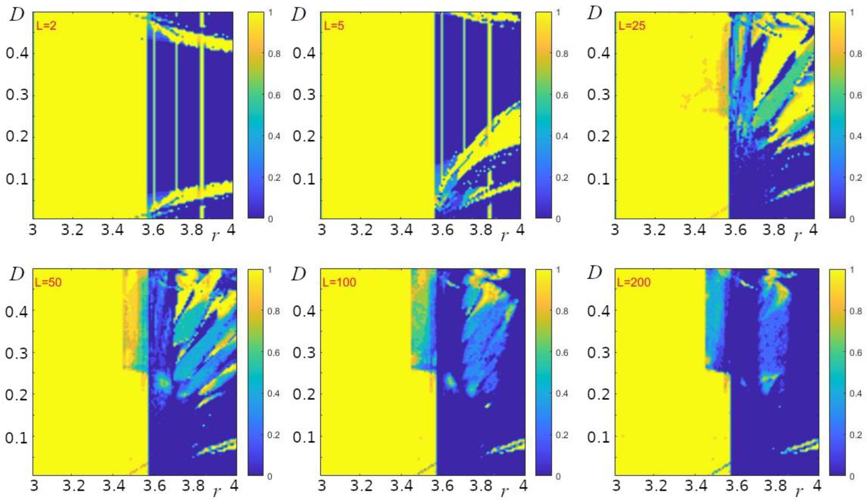
Figure 4.
Values of the averaged spatial entropy for different lengths (L = 50, 100, 200) of the oscillator chain (1) under different initial conditions (100 numerical experiments for each pair of the parameters r and D) (see Methods). The white color indicates the regions in which the values of x in all oscillators are the same at the end of computations.
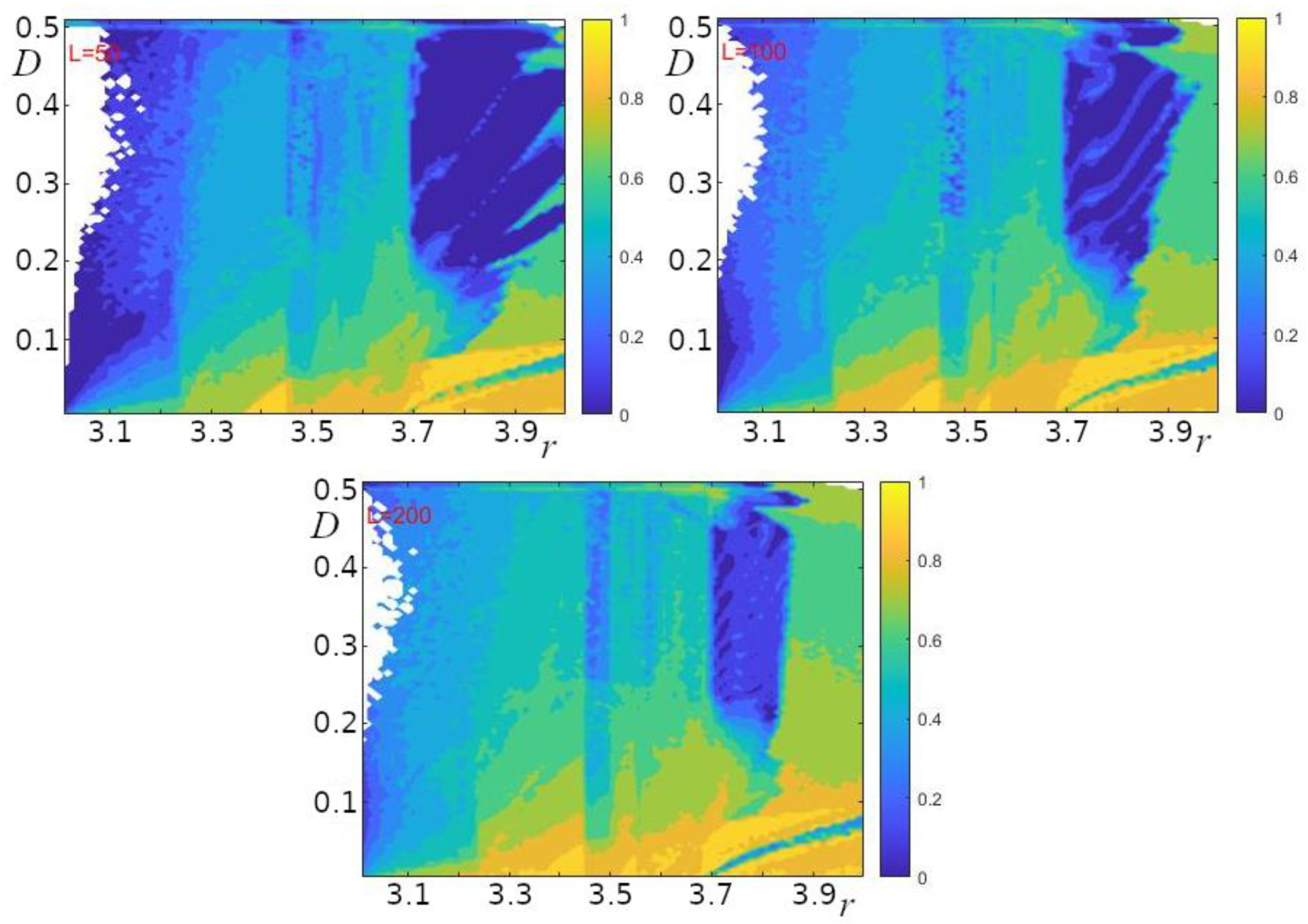
Figure 5.
Averaged values of
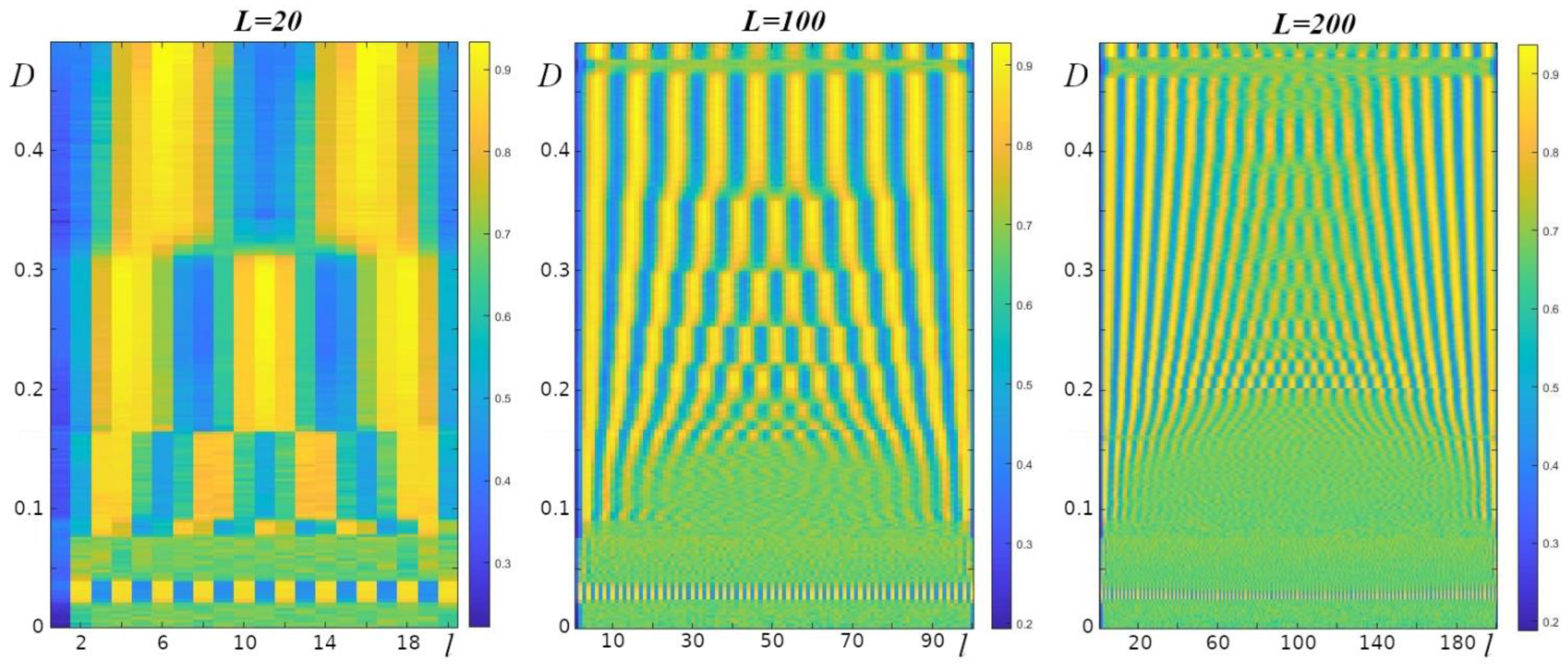
Figure 6.
The values of
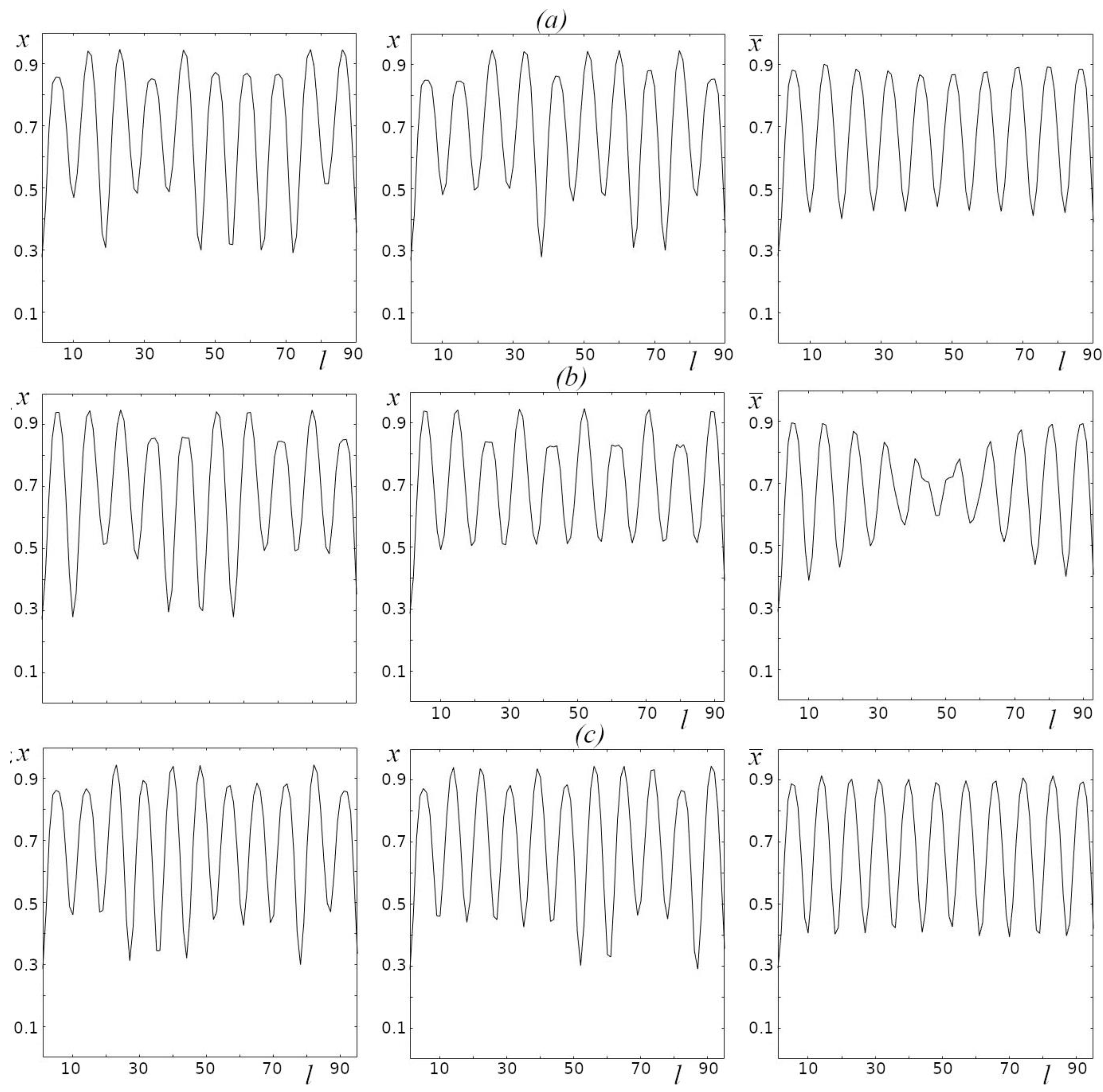
Figure 7.
Examples of spatial structures for different initial conditions (first and second columns), average values of
Figure 7.
Examples of spatial structures for different initial conditions (first and second columns), average values of
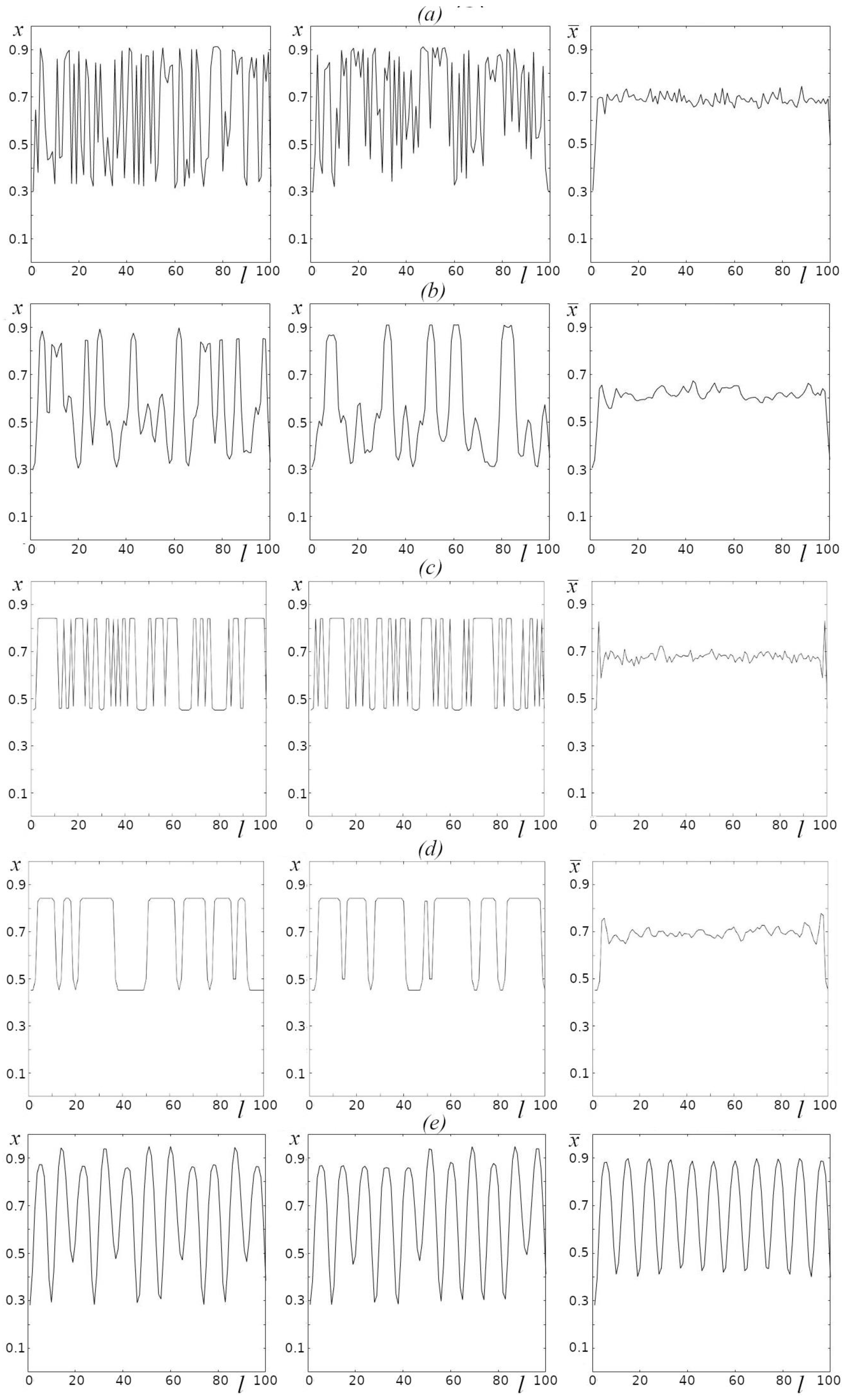
Figure 8.
Structure of the chain of coupled oscillators.
Disclaimer/Publisher’s Note: The statements, opinions and data contained in all publications are solely those of the individual author(s) and contributor(s) and not of MDPI and/or the editor(s). MDPI and/or the editor(s) disclaim responsibility for any injury to people or property resulting from any ideas, methods, instructions or products referred to in the content. |
© 2023 by the authors. Licensee MDPI, Basel, Switzerland. This article is an open access article distributed under the terms and conditions of the Creative Commons Attribution (CC BY) license (http://creativecommons.org/licenses/by/4.0/).
Copyright: This open access article is published under a Creative Commons CC BY 4.0 license, which permit the free download, distribution, and reuse, provided that the author and preprint are cited in any reuse.


