Advancements in Payments Does Influence Inflation Rate

Najla Saleh Albarrak; Hessa Abdulaziz Alsanousi

doi:10.20944/preprints202310.0351.v1

Submitted:

04 October 2023

Posted:

09 October 2023

You are already at the latest version

Abstract

Inflation is a crucial macroeconomic indicator which measures changes in the general level of prices of goods and services. In recent years, a series of successive events affected the inflation rates. To fight this increase in inflation, governments start to take different actions through their monetary and fiscal policies. In this research 10 independent parameters were used to see their effect on inflation rates. Some are traditional like GDP, Population, and exchange rate while others are some new technology related parameters like E-money payments transactions and number of Institutions offering payment services/instruments. The dependent parameter is the consumer price index (CPI). All parameters were taken in 8 years period (2013-2020). Supervised machine learning is used to run a robust regression model. The results show that technology advancement in payments is not a catalyst for price inflation if it is used properly and under regulations and control monetary policies. The results direct regulators to have a good understanding of the situation and take the right action in their policies of adopting fintech businesses.

Keywords:

Fintech

;

machine learning

;

monetary policy

;

inflation controls

Subject:

Business, Economics and Management - Finance

Introduction and Literature review

The world is witnessing rapid changes in inflation rates, specifically in recent years, inflation rates were affected by sequence compounding issues. Since COVID-19 pandemic, more specifically in mid-2021, the inflation rates started to rise to reach 4.7 percent. Many countries have registered their highest inflation rates at that period due to energy and food high costs. There are many drivers that might provoke the inflation rate such as supply and demand, unstable economy due to war, poor fiscal and monetary policies by governments, customer insecurity and many other factors. In 2022, the Russian – Ukraine war resulted in high oil prices which also worsen the situation and the global inflation is estimated to have reached 8.75 percent (O’Neill, 2023). This continued increase in the inflation rate, if not treated carefully will cause a cost-of-living crises for many individuals across the world. This drives us to conduct this research investigating the main factors to control this increase in inflation. New technologies have led to the creation of new electronic payments channels and lots of new Institutions offering payment services/instruments. Therefore, this advancement in technology will facilitate the purchases that might worsen the inflation rate in the future, in this study we shed the light on two important factors, along with other parameters, which are the transactions in electronic payment channels and the appearance of the E-payment companies to address the advancement in technology on the inflation level.

Previous study results by (KOÇ & ŞAHIN, 2021) show that both the volume and number of payment transactions have effects on inflation. A central bank is highly focus on payments systems for regulate the price level with the interest rate and liquidity strategies (Rumelili, 2006). As the range and variety of products in payment systems increases, the non-cash transactions also increase (World Payment Report, 2019). In several studies, it is argued that payment systems increase the rapidity of money by increasing the number of transactions (Geanakoplos and Dubey, 2010; The Perryman Group Report, 2015; Schoellner, 2002). The increase in the rapidity of money will also impact the general price level thus inflation rates. The new development in technology led to an increase in the use of financial advances systems which reduces liquidity in the economy while increasing the circulation rate of money. The progress in payment system causes changes both in money supply and money demand and thus make the money supply a dependent variable which is so difficult to trace and control. This condition causes a more difficult environment for the central banks which are trying to achieve price stability (Goldfeld and Sichel, 1990; Kogar, 1995; Oktayer, 2011).

Another study by monetarist school, reveals that the growth of money supply is the main factor in economic activity and inflation (Friedman and Schwartz, 1963; Mishkin, 2010). If the increase of the money supply surpassed the increase in money demand, the level of prices will increase (KOÇ & ŞAHIN, 2021). Also, an earlier study said that the common determinants of inflation for Asian countries like the exchange rate, real interest rate, deposit interest rate, annual GDP growth and broad money GDP have a negative impact on inflation (Ben Romdhane et al., 2023). On the other hand, some researchers believe that financial technology have a positive impact on inflation. They trust that the active consumption of Fintech through the two-way transactions (sale and purchase) settled by the digital payment made or received has a decreasing effect on inflation. However, inactive use through the simple action of buying or consuming such as using the internet to pay, made digital payment and debit card have a positive and significant impact on inflation. It has been suggested that, to make economic growth, the decision makers of the countries should improve their technological abilities and digital infrastructure. Also, regulators in these countries should launch an innovative environment and function through Fintech to assure consumer protection and financial stability.

In this research we contributed to knowledge by introducing a new factor which is the number of Institutions offering payment services/instruments and payments done through different type of cards. As well, we aim for applying robust regression, a machine learning model, on the panel data obtained from BIS statistics.

Research data

In this study we used the consumer price index (CPI) as the dependent variable for the robust regression. First, we calculated the yearly averages from monthly data and then we compare it to previous year to get the percentage change. The independent variables for this study are:

GDP: Nominal (USD per inhabitant)
Population: end of the year if available, otherwise average (thousands)
Exchange rate: end of year (Per USD)
Card and e-money payments: volume of transactions by card with a debit function
Card and e-money payments: volume of transactions by card with a delayed debit function
Card and e-money payments: volume of transactions by card with a credit function
Card and e-money payments: E-money payments
Banknotes and coins in circulation: Total value (USD bn)
Institutions offering payment services/instruments: Number of institutions.

The data gathered for this study is panel annual data from the data available at BIS Statistics Explorer website (BIS - Locational banking statistics). The period range of the study is 2013-2020 and for the following countries: Argentina (AR), Australia (AU), Belgium, Brazil (BR), Canada (CA), China (CN), France, Germany, Hong Kong SAR (HK), India (IN), Indonesia (ID), Italy, Japan, Korea (KR), Mexico (MX), Netherlands, Russia (RU), Saudi Arabia (SA), Singapore, South Africa (ZA), Spain, Sweden (SE), Switzerland (CH), Turkey (TR), United Kingdom (UK), United States (US), Euro area. Given the type and size of data we have, we establish a 216 number of observations for the model sample size.

Methodology:

In this research paper we used MATLAB to apply supervised Machine learning. We utilized the robust linear regression (fixed effect within estimator) given that it is less sensitive to outliers than standard linear regression. Standard linear regression uses ordinary least-squares fitting to calculate the model parameters that narrate the response data to the predictor data with one or more coefficients. As a result, outliers have a huge influence on the fit, because squaring the residuals expands the effects of these extreme data points. Models that use standard linear regression are based on certain assumptions such as a normal distribution of errors in the observed responses. If the distribution of errors is asymmetric or disposed to outliers, model assumptions are invalidated, which lead to that the parameter estimates, confidence intervals, and other computed statistics become undependable.

Robust regression uses a method called iteratively reweighted least squares to allocate a weight to each data point. This method is not as much of sensitive to large changes in small parts of the data. As a result, robust linear regression is less sensitive to outliers than standard linear regression. In weighted least squares, the fitting procedure includes the weight as an additional scale factor, which progresses the fit. The weights regulate how much each response value influences the final parameter estimates. A low-quality data point, for example an outlier, should have less influence on the fit. In order to achieve the best fit, the algorithm follows the following technique.

After weighting the model by least squares, the adjusted residuals are calculated and given by

r_{a d j} = \frac{r_{i}}{\sqrt{1 - h_{i}}}

Where

r_{i}

are the ordinary least-squares residuals and

h_{i}

are the least-squares fit leverage amounts. Leverages adjust the residuals by dropping the weight of high-leverage data points, which have a large consequence on the least-squares fit. As a result, the residuals are standardized as

u = \frac{r_{a d j}}{K_{s}} = \frac{r_{i}}{K_{s} \sqrt{1 - h_{i}}}

where

K

is a modification constant, and

s

is an estimate of the standard deviation of the error term given by

s

= MAD/0.6745.

MAD is the Median Absolute Deviation of the residuals from their median. The constant 0.6745 makes the estimate balanced for the normal distribution. If the predictor data matrix X has

p

columns, the model eliminates the smallest

p

absolute deviations when calculating the median.

The following step is calculating the weights

w_{i}

as a function of

u

. Where the bi-square weights are given by

w_{i} = \{\begin{matrix} {(1 - u_{i}^{2})}^{2} & , |u_{i}| < 1 \\ 0 & , |u_{i}| \geq 1 \end{matrix}

Then the model estimates the robust regression coefficients

b

. The weights calculation explained earlier will modify the countenance for the parameter estimate

b

as follows.

b = \hat{β} = {(X^{T} W T)}^{- 1} X^{T} W_{y}

Where

W

is the diagonal weight matrix,

X

is the predictor data matrix, and

y

is the answer factor. From there, the model estimates the weight least square error.

e = \sum_{1}^{n} w_{i} {(y_{i} - \hat{y_{i}})}^{2} = \sum_{1}^{n} w_{i} r_{i}^{2}

where

w_{i}

are the weights,

y_{i}

are the observed responses,

{\hat{y}}_{i}

are the fitted responses, and

r_{i}

are the residuals. The model will continue until fit converges or the maximum number of iterations is reached. Else, perform the next iteration of the least-squares fitting by returning to the computation of the adjusted residuals.

Results and Analysis

Given that the method used in this study is Fixed effects method; uses panel data to control for variables that differ across countries but are constant over time. We assume that characteristics of a country may impact or bias the predictor or outcome variables, and we need to manage this by using a fixed effect method. Fixed effects eliminate the effect of those time-invariant features, and therefore, we can assess the net effect of the interpreters on the dependent variable.

In fixed effects models, the coefficient of the population regression is the same for all countries, but the intercept of the regression line varies across countries (Stokes and Watson, 2019). Fixed effects (within) is the more generally used estimator for fixed effects models as it uses time difference within each cross-section. The following table shows the model regression results.

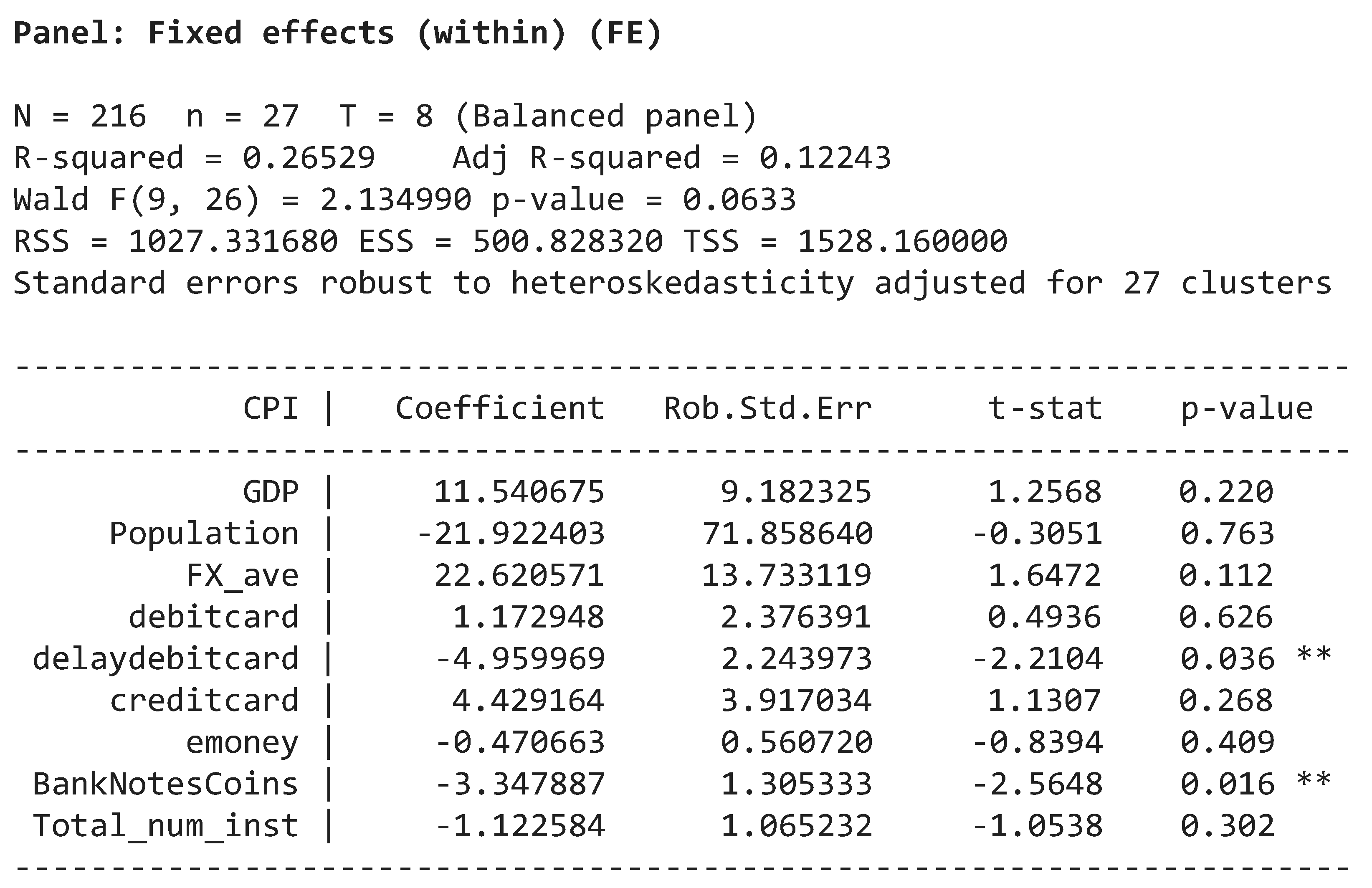
R-squared is a statistical measure that specifies how much of the difference of a dependent variable is explained by an independent variable in a regression model. In other words, 26% of the increase in CPI is justified by the model as seen in the R-square result from the table above. (Falk and Miller 1992) suggested that R-square values should be equal to or greater than 0.10 for the variance explained of a particular dependent variable to be considered adequate. (Cohen 1988) suggested R-square values for dependent variable are evaluated as follows: 0.26 (substantial), 0.13 (moderate), 0.02 (weak). Therefore, this study result shows a substantial evaluation of the dependent variable. On the other hand, recent studies suggest that the higher the R-square the better for linear regression uses Ordinary Least Squares (OLS). But since our model uses Robust regression which implies Iteratively Reweighted Least Squares (IRLS) for Maximum Likelihood Estimation (MLE), it is not that efficient measure to assess the fitness for robust regression by R-square only. R-square involves computing squared loss; sum of residual squared; squaring the sum of difference between predicted values and observed values in the formula for r-squared. So, robust regression includes dealing with data holding many outliers. The metric will result in illogical value due to large values produced from residuals for outliers which are large, hence, squared. Therefore, p-value figures have also been taken into consideration while evaluating the model. P-value of 0.06 indicates a statistically significant model.

Regarding Wald test, the model result has extent larger than the benchmark of 1.96, 2.13 for our model. Therefore, the coefficients of the variables are statistically significant (at the 95% level).

In analyzing the independent variable significance on the dependent variable, a p-value < or = 0.05 is considered statistically significant. Results show that the total Value of Bank Notes and Coins and Delayed Debit Cards are considered statistically significant in affecting inflation since their p-values are 0.016 and 0.036 respectively.

Both mentioned variables have a negative relation with inflation due to the negative coefficient results. A negative coefficient suggests that as the independent variable increases, the dependent variable tends to decrease. Therefore, the model shows that when the Total Value of Bank Notes and Coins increases by 1 USD billion, CPI annual change will decline by -3.34%. This result was not expected; it is common that high money in circulation is a signal to increase demand for purchases which will cause products’ prices to increase; inflated prices. But the result of this study shows the opposite.

Furthermore, the availability of further options of payments, especially with buy-now-pay-later, might also influence inflation as seen in Delayed Debit Cards transactions causing inflation to decrease by -4.9% annual change when volume of Delayed Debit Cards transactions increases by 1 million annually. Given that the holders of this type of card will delay their payments to a later time, this might help to reduce the money circulation now which result in lower CPI index in recent periods.

On the other hand, although Credit Cards transactions have large p-value of 0.268 however it has a positive relationship with CPI despite the similar option of buy-now-pay-later seen in Delayed Debit Cards transactions. Where an increase of 1 million yearly of Credit Cards transactions volume will increase CPI by 4.4% annually. This could be justified by the interest incurred for the delay payments in Credit Cards transactions through buy-now-pay-later option.

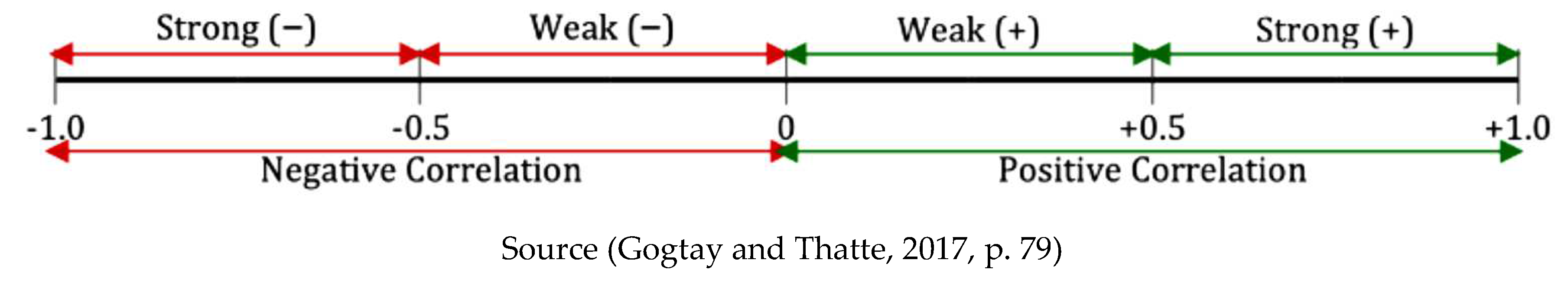
The results contradict the general knowledge that high liquidity increases inflation; therefore, this study considered the role of monetary policy actions by central banks rate movements and its impact on CPI. The percentage change in CPI figures in this model is a result of multiple actions in increasing/decreasing central banks rate by countries under study. We took each country’s CPI annual changes and its end of year discount rate annual changes and based on the relationship result between CPI and policy rate, the degree of correlative measure can be Positive, Zero or Negative correlation. If the sloping of the differences in CPI and policy rate is positive and almost equal to 1, there may be probability to have positive connection of each other and such association can provide positive correlation coefficient. And if the trend of the differences is negative, such suggestion can result in negative correlation coefficient. Basically, the coefficient of correlation will range between -1 and +1. According to (Gogtay & Thatte, 2017), the correlation coefficient can be read based on its rate as in

The following correlation result table indicates the relation between difference in CPI and difference in policy rate lagged by 1 year.

From the correlation result table above, the most effective response in CPI due to central banks rate changes are highlighted. The gray highlight indicates the highest negative relation with CPI per country and the blue highlight indicates the highest positive relation with CPI per country. In general, results showed a medium to high correlation between the changes in discount rates and the inflation rates. For example, in year 1, results shows that countries like India, Korea, Saudi Arabia, Sweden and UK shows a high negative correlation between the two variables: increase in discount rate % changes led to decrease in CPI % changes. Another example, in year 0, countries like Australia, Brazil, Hong Kong, Turkey and US have a positive relation between discount rate and inflation. This fact indicates that there are other factors that might influence CPI than policy rate.

Consequently, our results signal that the control of the inflation rate is not subject to specific parameters but its attainable with appropriate monetary policy actions. Economically, countries could inhabit the development in financial technology solutions to an extent without incurring economic deficiency.

Conclusion

In conclusion, the global inflation rate has jumped to a new level that has not been seen for decades, which encourages us to focus on the parameters that might help to control such increase in prices. Nowadays, technology has contributed to the spread of advancement in payment systems. This development might influence the inflation rate due to facilitating the spending behavior for individuals and shift towards more non-cash payments. Therefore, we contributed to knowledge by adding technology related parameters to our study.

Our Findings implies that the technological development in electronic payment services and has direct relationship by a negative impact on inflation prices. This could be justified by fixing the price of purchases albeit the delayed installments. Unlike the higher prices paid through incorporating interests by credit cards purchases.

To control inflation, the Government should focus on balancing each parameter that might affect the increase in prices along with appropriate fiscal and monetary policy. They also should focus on innovation and technology to facilitate and speed information and action needed to keep the inflation rates within acceptable levels. As well, appropriate security and legislations should gain high importance due to cross boarder payment services.

References

Ben Romdhane, Y. , Kammoun, S. and Loukil, S. (2023), "The impact of Fintech on inflation and unemployment: the case of Asia", Arab Gulf Journal of Scientific Research, Vol.
Cohen, J. (1988). Statistical power analysis for the behavioral sciences (2nd Ed.). New York: Routledge.
Falk, R. F. , & Miller, N. B. (1992). A primer for soft modeling. University of Akron Press.
Friedman, M. and Schwartz, A. J. (1963). Money and Business Cycles. Review of Economics and Statistics, 45(2), 32-64. 2.
Geanakoplos, J. and Dubey, P. (2010). Credit cards and Inflation. Games and Economic Behaviour, 70, pp. 325-353.
Gogtay, N. J., & Thatte, U. M. (2017). Principles of correlation analysis. Journal of Association of Physicians of India, 65(MARCH), 78–81.
Goldfeld, M. and Sichel, D. (1990). The Demand for Money. In B. Friedman and F. Hahn, Handbook of Monetary Economics (pp. 299-353). New York: North-Holland.
KOÇ, Ü. , & ŞAHIN, H. (2021). The Role OF Electronic Payments in Inflation Dynamics. International Journal of Economic & Administrative Studies, Issue 32, p1-15.
Kogar, Ç. (1995). Financial Innovations and Monetary Control. The Central Bank of the Republic of Turkey, Research Department, Discussion Paper, No: 9515.
Mishkin, F. S. (2010). Will Monetary Policy Become More of a Science? In V. Wieland, The Science and Practice of Monetary Policy Today (pp. 81-103). Berlin, Heidelberg: Springer.
O’Neill, A. (2023). Global inflation rate from 2000 to 2028. Retrieved from https://www.statista.com/statistics/256598/global-inflation-rate-compared-to-previous-year/#:~:text=A series of compounding issues, increase in inflation since 1996.
Oktayer, A. (2011). Financial Innovations and Money Demand. Maliye Dergisi, 160, 351-368.
Rumelili, Ö. M. (2006). Information Technology Risks in Payment Systems. Ankara University, Unpublished master thesis.
Schoellner, T. (2002). The Effects of Credit Cards on Money Demand. Unpublished Ph.D Dissertation, Ohio State University.
The Perryman Group Report. (2015). The Electronic Payment System: An Assessment of Benefits for the US and State Economies. The Perryman Group.
World Payment Report. (2019). Capgemini World Payments Report 2019. Capgemini Research Institute.

Disclaimer/Publisher’s Note: The statements, opinions and data contained in all publications are solely those of the individual author(s) and contributor(s) and not of MDPI and/or the editor(s). MDPI and/or the editor(s) disclaim responsibility for any injury to people or property resulting from any ideas, methods, instructions or products referred to in the content.

© 2023 by the authors. Licensee MDPI, Basel, Switzerland. This article is an open access article distributed under the terms and conditions of the Creative Commons Attribution (CC BY) license (http://creativecommons.org/licenses/by/4.0/).

Copyright: This open access article is published under a Creative Commons CC BY 4.0 license, which permit the free download, distribution, and reuse, provided that the author and preprint are cited in any reuse.