

Submitted:
30 September 2023
Posted:
30 September 2023
You are already at the latest version
Abstract
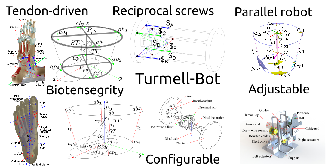
The ankle is a complex joint with a high injury incidence. Rehabilitation Robotics applied to the ankle is a very active research field. We present cable-driven reconfigurable robot kinematics and statics. We studied how the tendons pull mid-foot bones around the talocrural and subtalar axes. Likewise, we propose a hybrid serial-parallel mechanism analogous to the ankle. Then, using screw theory, we synthesized a cable-driven robot with the human ankle in the closed-loop kinematics. We incorporate a draw-wire sensor to measure the axes’ pose and compute the product of exponentials. We reconfigure the cables to balance the tension and pressure forces using the axis projection on the base and platform planes. Likewise, we also computed the workspace to show that the reconfigurable design fits several sizes. The data used is from anthropometry and statistics. Finally, we validated the robot’s statics with MuJoCo for various cable length groups corresponding to the axes’ range of motion. We suggested a platform adjusting system and an alignment method. The design is lightweight, and the cable-driven robot has advantages over rigid parallel robots, such as Stewart platforms. We will use compliant actuators.
Keywords:
medical and rehabilitation robotics
; biomechanics
; parallel manipulator
; cable-driven
; kinematic analysis
; robot design
; mechanism synthesis
; compliant mechanism
1. Introduction
The ankle is a complex joint with high injury incidence. There are growing research interest in robotics to assist ankle rehabilitation. Our purpose is to create a device that can aid in the movement of the human ankle joint by restoring its range of motion. We focused on the reconfigurable kinematics, statics, and adjustable design.
In this work, we have taken a human-centered approach [1,2,3,4,5,6,7,8,9,10,11]. We propose an adjustable device for different foot sizes and be able to switch between limbs. The design is for the patients in lying down positions. Our approach is to mimicry the tendons involved in ankle movements while avoiding any forces that could pull the foot away from the ankle. We propose reciprocal tendons that apply pressure against the plantar surface of the foot, which will induce ankle joint integration forces to generate motion.
1.1. Ankle Rehabilitation Robotics
There are many state-of-the-art articles, literature reviews, and design considerations related to ankle rehabilitation robotics. For example, we found designs based on platforms in [12], state-of-the-art techniques in [13], and robot-assisted therapy in [14]. We also found the state-of-the-art robot-assisted ankle neurorehabilitation and challenges reviewed in [15], a mechanical design review in [16], robot-assisted techniques reviewed in [17], and a home-based review in [18]. Furthermore, we found anatomy-based designs regarding ankle-foot robotics considered in [19], and research progress in [20]. In general, most of the efforts are focused on parallel mechanisms, which have advantages over serial counterparts[21] and can be analyzed by using screw theory [22,23], as is explained in modern robotics [24,25].
1.2. Cable-Driven Robotics
Cable-driven parallel mechanisms have lightweight designs acting in tension against gravity or mutual tension configurations. They are reviewed in [26] and [27] and studied in [28]. A state-of-the-art is discussed in [29]. Cable-driven robots were applied to human arms [30], with Bowden guides [31] in lower-limbs [32]. The idea of attaching the shank and the foot was discussed in [33]. Additionally, wires [34] and a cable-driven ankle rehabilitation robot, were used in [35]. Such mechanisms are related to tendon-driven mechanisms [36], musculoskeletal robots, and artificial muscles.
2. Materials and Methods
First, we study the ankle anatomy in [37] and the International Society of Biomechanics (ISB)[38]. Then, we use the open-source digital model (z-anatomy) [39] to identify the bones, insertions, tendons, and muscles related to the ankle movement. We introduced the dimensions and geometrical model in a Jupyter Notebook using a SageMath 10 kernel [40] in [41]. We provided the CAD model in [42] and the sources in GitHub [43]. We identified the tendons involved in ankle movement acting as an over-actuated bio-mechanism (two degrees-of-freedom and four tendon groups). Then, we choose antagonistic tendon groups. We identified the pressure forces from the platform against the plantar surface of the foot. Then, we drew a schematic with the tension forces between the base attached to the shank and a platform attached to the foot. We adapted the robot dimensions from [44], the proportions from [45], and the statistical data from [46].
We start the design by analyzing a simple cable-driven two-axis serial chain, which helps us to understand the reciprocal products between the cable and axis screw representations. We create artificial data from the ankle model using the forward kinematics computed from the “product of exponentials” (PoE). The data serve us to validate how to get the ankle model in practice from trajectory measurements received from a modification of the Turmell-Meter system [47]. When synthesizing the robot, we enlarged the device size to prevent cable contact with the body from the platform and base. We analyzed the cable-driven antagonistic actuation in the perpendicular axes model and use it for the initial calibration. Afterward, we propose a method for the robot reconfiguration, the workspace, and the static simulation using MuJoCo 2.3.1 [48] to validate the stability by changing the axis and tendon positions. Finally, we proposed a CAD model using SolidWorks 2022.
2.1. Robot Inspired on the Analysis of the Ankle Joint
The model has two rotational joints and four tendons involved in ankle movement. First, we analyzed the tension forces and then the compression forces. Finally, we propose a simplified schematic for the robot.
2.1.1. Ankle-Foot Tendons
The two-axis representation and the tendon insertions in the bones at the mid-foot are in Figure 1. The Figure 1 illustrates the main tendons from the lateral-anterior view of the right foot. As we show in Figure 1, the fifth metatarsal has two insertions, the peroneus tertius, with components for dorsiflexion and eversion, and the peroneus brevis, for eversion and plantarflexion. The calcaneus has the insertion of the Achilles tendon for inversion and plantarflexion. In Figure 1, we show the medial-bottom view of the foot, and the insertion points are between the first metatarsal and the medial cuneiform. The tibialis anterior contributes to inversion and dorsiflexion, the peroneus longus contributes to plantar flexion and eversion, and the tibialis posterior contributes to inversion and plantar flexion.
2.1.2. Foot Compression Forces
Some requirements for ankle rehabilitation are security and comfort. The foot supports high compression forces in some regions of the plantar surface. In contrast, the dorsal skin is thin, soft, and less tolerant of compression forces. We propose a device that mainly applies pressure at the plantar surface to integrate the ankle joint and generate motion. From the bottom view of the foot, we note that the pressure points are involved in the subtalar and talocrural axes motion. The Figure 2 shows the axes projection and the triangle vertices of the transversal plane. The three main points are the tubercle of the calcaneus and the first and fifth metatarsal heads. The pressure points are the projection of the triangular-shaped dome, limited by the lateral, medial-longitudinal arches, and the anterior transverse arch. These contact points transmit a compression force to the platform.
2.1.3. Robot Based on the Ankle-Foot Model
We designed a reconfigurable cable-driven robot to actuate on synergy with the ankle tendons. Cables from the base pull the platform attached to the foot. The cable anchor points have a relocation mechanism to equilibrate the rotation forces on the ankle joint. We align the centers to the ankle axes’ intersection on the transverse plane. We show the schematic design in the Figure 3. In Figure 3, we sketch the approximated schematic and show the tendon directions regarding the subtalar (ST) and the talocrural (TC) axis. We represent the foot platform with a circle with a radius , centered on , and on the same plane of the anchor points , , , and . The base is a circle with a radius in the same plane as , and the anchor points , , , and . We simplified the plantar surface of the foot with three contact points , , and . Finally, , , and are tendons. The serial kinematic chain is RR, starting at the origin , followed by a rotational joint at on the TC axis, followed by the link to a rotational joint at on the ST axis. A link from to connects the platform with the ankle. The tendons from , , , and on the platform to the corresponding , , , and on the platform complete the parallel closed-loop structure. Each human ankle has different axis positions; thus, we propose reconfigurable cable attachments. In Figure 3, the green arrows illustrate the concept of reconfiguration for the right foot by displacing the anchor endpoints , , , and on the platform and the anchors , , , and on the base. We designed a mechanism for centering pivot points and .
We computed the center points from the intersection of the talocrural and subtalar axes projected on the transverse plane parallel to the base and the platform. Such pivot points are not the same as and , which pertain to the position sensors reference system.
2.1.4. Dimensions and Initial Configuration
In this section, we estimate the initial robot size and configuration. We use the ankle model and measurements from [44], human proportions from [45] and statistical data from [46]. We show the proportions in Figure 4. The TC axis is dominant, and we use its statistical value for the cable-body collision analysis. We simplified the body as a sphere centered in half of the ankle’s most medial point (MMP) and most lateral point (MLP); between the two malleoli. We compare this dimension with a leg model in Figure 4b, illustrating the distance between the ankle and PM on the platform. Additionally, we show that the cables must not be in contact with the foot or the malleolus. The sphere represents the radius between the ankle and the plantar surface of the foot.
2.2. Ankle Kinematic Model
For the ankle kinematics representation, we used data from a two-axis model representation of the ankle joint explained in [47]. There, we described a system for platform pose capture and a method for model approximation using circle fitting, the Figure 5 shows the concept.
The points , , and are references on the talocrural axis. Similarly, , , and are in the subtalar axis. We used it to compute the following vectors and matrices:
Then, we compute the Rodrigues’ formulas:
representing the and rotations about and , respectively. Also, we compute the matrices:
where:
If we define the initial pose representation as:
where:
where each column vector is:
Then, we finally get the product of exponentials (PoE) representation for the serial chain with two hinge joints for all the P points on the platform:
where is the total rotation matrix and is the total translation vector.
The model formulas are in the Appendix A.1.
2.3. Synthesis of the Parallel Tendon-Driven Robot
The cables must not be in contact with the body and be smaller than the base and platform used by the draw-wire sensors. To simplify the collision study, we analyzed a coronal section of the foot and ankle, and the contact body is a circle containing the ankle, as illustrated in Figure 6. We use this coronal section to approximate the platform and base sizes. In Figure 6, two tendons drive a hinge joint, and the platform anchor points trace two concentric circular trajectories. The segments and represent two antagonistic tendons, is the radius of a solid body containing the axis of rotation, and the interior circle represents a solid body. The collision contact of the cable with the body depends on the base and platform proportions and the radius . By observing, we note that if the base is larger than the platform, we can enhance the range of motion of the hinge joint. The points , , and are references on the talocrural axis. Similarly, , , and are in the subtalar axis. We used it to compute the following vectors and matrices:
We use this coronal section to approximate the platform and base sizes. From the initial position, we define a maximum and minimum reached angle. In Figure 7, we illustrate the full range of motion of the platform.
The limits are due to collision between the cables and the base body. When is extending and is contracting, Tendon touches the foot in . The minimum angle is limited for such a collision. The maximum angle occurs when is contracting and is extending. We select a radius greater than the foot width, and then we evaluate a platform radius greater than the radius. By selecting a base radius , we can evaluate the range of movement. The positive arc and its derivate are:
The derivative is the slope of the line in the tangent point :
solving for y yields:
We found the tangential point by substituting y from Equation (18) in Equation (21) (22), and simplifying yields (23):
To solve for , we use the software SageMath 10.0. Then, we replace the positive value in Equation (18) to find .
Finally, we found the intersection with the circular trajectory that has a radius . To solve for , we use the following equation:
We found by replacing in Equation (18).
To find the arch length, we consider the initial position of anchor point on the platform. We use the following Equation:
where is the length from the circle center to the platform central point and defines the trajectory radius regarding the positive semicircle. We solve for yields two values. By selecting the positive value, we obtain . The arc length is given by the absolute difference of the two corresponding angles. We computed the angles by using the Equation:
2.3.1. Cable-driven Two-Rotational Serial Chain.
In this subsection, we study a model in three dimensions that is analogous to the ankle joint. The model uses the screws in an antagonistic configuration to achieve tension forces at the cables. In the Figure 8, the view is normal to the proximal axis, and the Figure 8 shows the normal view of the distal axis.
We use this simplified model to compute the cable locations. Also, we can use the model for testing and calibrating the mechanism before use in humans. With the purpose of designing a reconfigurable physical model, we represent the rotational joints as axes located coincident in opposite edges on a tetrahedral structure, as shown in Figure 9. We choose two different configurations by rotating the anchor points by (half of ) from their initial position on the base and the platform. The first coincides with the rotation axis as in Figure 9, the second configuration is similar to that observed in the ankle, and we show this configuration in Figure 9.
The first representation allows us to visually identify the intersection points between the tendons’ lines of action.
Such a condition results in null reciprocal twists because they are coplanar [49]. So the reciprocal products are:
This configuration must be avoided because it leads to a singularity.
The relations for all the tendons on the rotary joints are as follows:
In the Figure 9, we show the following:
Then, the sum of all reciprocal products is zero, which means that the platform is in a static position. However, it is unstable because little variation in the anchor position suddenly changes the product’s sign. In the second configuration, the twist pair and is antagonistic with regards to and about the proximal twist . Also, and are antagonistic with respect to and about the twist . We will use this in our design.
In summary, two conditions are important to avoid: singular configurations and cable collisions. We address the first condition by changing the angle position of the anchor points and the second condition by selecting the base and platform radiuses bigger than the foot standard size.
2.4. Robot Configuration
For simulation and validation, we generate trajectories and capture the axes pose using the formulas in the Appendix A.2 and Appendix A.3. The method uses the formulas in the Appendix A.4 for selecting the trajectories. The axis approximation formulas are in the Appendix A.5. Finally, the range of motion and the common perpendicular line are in the Appendix A.6 and Appendix A.7 complete the captured bi-axial model characterization. This data are important for the minimum and maximum cable lenghts computation.
We assume that the base plane is parallel to the transversal plane of the shank. With the reference systems aligned and and centered on the base and the platform. The shank line is perpendicular to the foot plane, and the neutral position occurs when the four tendons have similar tension. Therefore, the actuators used in antagonistic operation will have seamless forces. When the platform of the foot is parallel to the transversal plane of the shank, the talocrural and subtalar axes projected to the plane in symmetric form are:
Solving for y yields:
Subtracting (35) from (34), we have:
Solving for x yields:
We create two planes parallel to the z-axis, coincident with the intersecting point :
where the normal vectors are:
We compute the angle between the planes. This equation can be used to calculate the minimum and maximum angles, and the angles can be obtained as follows:
We rotate the unitary vector normal to the planes and about an axis parallel to the z-axis and pass it through . The resulting vectors are:
where is the unitary vector in the direction of the positive z-axis.
The resulting lines in symmetric form are:
Then, we obtain the pivot point on the robot platform, and the pivot point on the base, corresponding to projected on the platform and the base. The platform and base attachment points are at the intersection between the circle centered on the pivot points and with the lines of Equations (44), the circle equations are:
The platform radius is , and the base radius is . By solving for y in (44), substituting it in (45), and solving for x, we can obtain the following two values:
where:
Substituting these values back into Equation (44) yields:
- Then, by substituting by , we can obtain the other two points. Finally, we obtained four points for the platform. Obtaining the base anchor points is similar to computing the platform anchor points, replacing by , and by we compute four base corresponding points. The reconfigurable structure is easy to set up by changing the angle position given by:where and are the corresponding angles of each anchor point on the platform and the base related to the x direction around the intersection projected points and .
3. Workspace From the Product of Exponentials
By knowing the platform’s initial configuration, we can plot the anchor point group of movements from the product of exponential matrices by applying the Equation 17 to each platform anchor point. The product of exponential matrices for each anchor point on the platform is:
Moreover, the cable lengths can be calculated as follows:
The range of the talocrural angle is , and the subtalar angle range is The surfaces represent the group of movements for each anchor point on the platform.
3.1. Reconfiguration and Statics Simulation
The robot configuration depends on the ankle axis location. We compared the analogous two-axis system and the ankle biaxial model on MuJoCo 2.3.1. We used this software because it is open-source and free to use. Additionally, it is used for model-based control. We provided the XML source in [43]. The simulation process is easy, we edited the tendon lengths in the text editor and reloaded the simulation in MuJoCo 2.3.1. We stopped the simulation, we changed the hinge joint angles, then we ran the simulation with the computed tendon lengths. The simulation stops in a static position at previously computed angles.
4. Results
4.1. Base and Platform Dimensions.
First, we show the resulting base radius in Table 1 with a relation . Every module has radius .
The draw-wire sensor modules are in the base, we compute the position of each module by translating the origin centered triangle with vertexes , , and in Table 2.
The base reference vertexes are in Table 3.
We can generate sensor lengths for the synthetic data generation by subtracting points pertaining to the groups from the corresponding module vertexes. For example, we get the distance between the initial position from to the module .
We do the same for all points, then we have the lengths from each initial point tho the corresponding sensors in Table 4.
4.2. Trajectories From the Group of Movements.
In this subsection, we use synthetic trajectories generated from the product of exponential matrices. We take 50 samples for each generated trajectory and obtain the plane containing the trajectories in Table 6.
The resulting circle-fitting estimation is in Table 7.
We compute the mean rotation axis and the mean axis and center. The rotation axis and trajectory center are in Table 8.
We apply a similar method for the subtalar axis estimation, then we summarize the resulting normal vector, angle, and axis regarding the plane parallel to x-y in Table 9.
The resulting circle-fitting estimation is in Table 10.
The mean rotation axis and mean trajectory center for the talocrural axis are in Table 11.
We summarize the resulting characterization compared to the provided by the synthetic data and the minimal distance error in Table 12.
4.3. Talocrural Range of Motion.
In this subsection we use decimated data for illustrative purposes. First, we divided the trajectories in two groups. From the initial position reference we separate the negative and the positive angles. The Table 13 shows the negative angle group.
The points differences for negative angles are in Table 14.
The rotation matrix vectors components are in Table 15.
The rotation matrices and the angles are in Table 16.
The greatest negative value is 0.34906 radians, corresponding to . The positive values start from the initial position tho the trajectory end, are in Table 17.
The points differences for the positive angles are in Table 18.
The rotation matrix components are in the Table 19.
The rotation matrices for the positive angles are in Table 20.
The greatest positive value is 0.34906, corresponding to . Then the total range of motion is .
4.4. Robot’s Platform and Base Sizes.
In this section, we select the platform, the base sizes and the location of the anchor points for mean values. We use Figure 7 and the Equation (26). The body segment is proportional to the human height H=1752 mm. The robot platform and base radius are smaller than the platform and base of the draw-wire sensor system.
We multiply the robot platform radius and robot base radius , where Pf is a factor from 50% to 100% of the sensor base and sensor platform.
The range of motion for different proportional values are in Table 21.
For H maximum, the angles are in Table 22.
For H minimum, the resulting angles are in Table 23.
For all three cases, we need at least for the angle, also a proportion near to the sensors or the foot is not desirable, we select a proportion of 80% from the base (0.8rb) and platform (0.8rp) of the draw-wire sensor system, then and , which are enough for the mean height H.
The Figure 10 shows the range for the mean, maximum and minimum heights.
4.5. Screws and Reciprocity Initial Analysis.
In this subsection, we analyze the platform screws system. We use Figure 9 as a reference, and then we build a model based on the cable anchor with the platform and base. Then, we reconfigure the anchor point places to rotation about the z unitary axis . The base and platform corresponding points are provided in the Table 24.
The resulting reciprocals are in Table 25.
We observe that in the 45° rotated configuration, each pair of cable-driven actuators works in the tensegrity mode. Additionally, it is possible to apply work from the cables in the tension to the rotation axes in the serial kinematic chain.
4.6. Projection of the Intersection Pivot Point.
The projected axis on the plane x-y, has a intersection point. We use the different axis attitudes for finding the intersection point. The results are in the Table 26.
4.7. Robot Configuration
We show how to align the robot at the initial projected pivot point intersection. It is imperative to align the references before placing the cable anchors on the platform and the base. For simulation, we use the ankle forward kinematics, common perpendicular, and range of motion in the Appendix B.1, Appendix B.2 Appendix B.3 appendix sections.
In the Figure 20, the horizontal and vertical guides have markers when the robot is centered with respect to the draw-wire sensor system. On the top-left side, we designed scales for fine alignment after patient-specific ankle-axis estimation. The pivot point depends on the anthropometric measurements; in this case, we use the standard deviation and the mean values for the common perpendicular distance Q=mean. The resultin projection points are in Table 27.
For Q maximum, we show the results in Table 28.
For Q minimum, the results are in Table 29.
We note that by changing the different parameters, the robot has sufficient range to reconfigure the anchor points. So the aligning system work with different axis attitudes.
4.8. Angle Computation of the Anchor Points
After we centered the robot around the intersection of the talocrural and subtalar axes projected on the base and initial platform planes, we configured the four cable anchor points. To do so, we use Equations (46), (47), and (48) to compute the anchor points. In this subsection, we only change the axis attitudes and then compute the anchor points. The Table 30 shows the resulting computed data for the axes’ mean, maximum, and minimum attitude values. We refer to the axes’ mean attitude when TC and ST have mean statistical values. Also, we call the maximal attitude when we add the standard deviation to the TC and ST means. The same goes for the minimum.
From this table, we compute the angle configuration of the attaching points in Table 31.
The angles for the base and platform anchor points for maximum attitude are in Table 32.
The angles for the base and platform anchor points for maximum attitude are in Table 33.
The Figure 11 shows the anchor points the three axes attitude groups.
4.9. Workspace
4.10. Cable Lenghts at Initial Position
We use Equation (51) to compute the cable lengths at the initial position.
The resulting lengths for the mean values are shown in the Table 34.
For the initial lenghts, we draw the forward kinematics is the intersection between four spheres and the circle representing the platform, with the pose represented on , as in the Figure 12.
4.11. Cable Lengths at Extreme Positions
We create three tables with different axis attitudes and compute the positions. The Table 35 shows and .
The Table 36 shows the anchor points , , , and .
The Table 37 lengths for the cables.
The Figure 13 shows the four configurations corresponding to axes’ mean attitude values.
The resulting platform position anchor points corresponding to the axes’ maximum attitude values are in Table 38.
The cable lengths corresponding to the axes’ maximum attitude values are in Table 39.
The Figure 14 shows the four configurations corresponding to the axes’ maximum attitude values.
The resulting platform position anchor points corresponding to the axes’ minimum attitude values are in Table 40.
The cable lengths corresponding to the axes’ minimum attitude values are in Table 41.
The Figure 15 shows the four configurations corresponding to the axes’ minimum attitude values.
4.12. MuJoCo Simulations
In this section, we replace the anchor points, the kinematic chain and the tendon lengths in the XML script included in the repository [43].
In the simulation, we rotate about the y-axis and scale the positions by a factor of 0.1. The units are in centimeters. The input values are in Table 42.
We put this model the XML document as in the Listing 4.12.
| XML MuJoCo file. |
| <?xml version="1.0" encoding="UTF-8"?> |
| <mujoco model="turmellbot"> |
| <compiler coordinate="local"/> |
| <default> |
| <geom rgba=".8 .6 .4 1"/> |
| </default> |
| <asset> |
| <texture type="skybox" builtin="gradient" rgb1="1 1 1" rgb2=".6 .8 1" width="256" height="256"/> |
| <mesh file="a-foot.stl" refpos="-10.84427 0.1037934 -17.62868" refquat="0.99619 0.034862 0.00000 0.00000"/> |
| </asset> |
| <worldbody> |
| <light pos="10 -10 50" dir="-10 10 -50" diffuse="1 1 1"/> |
| <site name="reference" pos="5.938405e-19 -0.09110710 17.62735"/> |
| <body> |
| <geom name="base" type="cylinder" fromto="-0.4000000 -0.09110710 17.62735 5.938405e-19 -0.09110710 17.62735" size="12.032592"/> |
| <site name="b1" pos="-6.093131e-16 6.659522 7.666812" size="0.2"/> |
| <site name="b2" pos="6.105008e-16 -6.841736 27.58788" size="0.2"/> |
| <site name="b3" pos="4.139506e-16 9.869429 24.37798" size="0.2"/> |
| <site name="b4" pos="-4.127630e-16 -10.05164 10.87672" size="0.2"/> |
| <geom name="leg" type="capsule" fromto="5.938405e-19 -0.09110710 17.62735 10.84427 -0.1037934 17.62868" size="0.3"/> |
| <site name="shnk" pos="10.84427 -0.1037934 17.62868"/> |
| <body> |
| <geom name="comp" type="capsule" fromto="10.84427 -0.1037934 17.62868 11.19642 -0.01170672 17.90907" size="0.3"/> |
| <joint name="TC" type="hinge" pos="10.84427 -0.1037934 17.62868" axis="-0.1740000 0.9790000 -0.1030000" limited="true" range="-20 20"/> |
| <body> |
| <geom name="b-foot" type="capsule" fromto="11.19642 -0.01170672 17.90907 17.61765 -0.09110710 17.62735" size="0.3"/> |
| <joint name="ST" type="hinge" pos="11.19642 -0.01170672 17.90907" axis="-0.6420000 0.2080000 0.7380000" limited="true" range="-15 15"/> |
| <geom name="ptfm" type="cylinder" fromto="17.61765 -0.09110710 17.627 18.01765 -0.09110710 17.62735" size="9.25584"/> |
| <site name="ptfmc" pos="18.01765 -0.09110710 17.62735" size="0.3"/> |
| <geom name="s-foot" type="mesh" mesh="a-foot" rgba=".85 .79 .72 0.7" density="0.01"/> |
| <site name="p1" pos="17.61765 5.101684 9.965397" size="0.2"/> |
| <site name="p2" pos="17.61765 -5.283899 25.28930" size="0.2"/> |
| <site name="p3" pos="17.61765 7.570844 22.82014" size="0.2"/> |
| <site name="p4" pos="17.61765 -7.753058 12.43456" size="0.2"/> |
| </body> |
| </body> |
| </body> |
| </worldbody> |
| <tendon> |
| <spatial name="t1" limited="true" range="17.83503 17.83513" width="0.05" stiffness="100" damping="100000"> |
| <site site="b1"/> |
| <site site="p1"/> |
| </spatial> |
| <spatial name="t2" limited="true" range="17.83503 17.83513" width="0.05" stiffness="100" damping="100000"> |
| <site site="b2"/> |
| <site site="p2"/> |
| </spatial> |
| <spatial name="t3" limited="true" range="17.83503 17.83513" width="0.05" stiffness="100" damping="100000"> |
| <site site="b3"/> |
| <site site="p3"/> |
| </spatial> |
| <spatial name="t4" limited="true" range="17.83503 17.83513" width="0.05" stiffness="100" damping="100000"> |
| <site site="b4"/> |
| <site site="p4"/> |
| </spatial> |
| </tendon> |
| <actuator> |
| <muscle name="t1" tendon="t1"/> |
| <muscle name="t2" tendon="t2"/> |
| <muscle name="t3" tendon="t3"/> |
| <muscle name="t4" tendon="t4"/> |
| </actuator> |
| <sensor> |
| <accelerometer name="ptfacc" site="ptfmc"/> |
| <gyro name="ptfgyro" site="ptfmc"/> |
| <tendonpos name="t1pos" tendon="t1"/> |
| <tendonpos name="t2pos" tendon="t2"/> |
| <tendonpos name="t3pos" tendon="t3"/> |
| <tendonpos name="t4pos" tendon="t4"/> |
| <jointpos name="TCpos" joint="ST"/> |
| <jointpos name="STpos" joint="TC"/> |
| </sensor> |
| </mujoco> |
There are bodies like the base and the platform, three links, two hinge joints, four tendons with sensors and actuators. The data configuration is from the simulation at the initial position. We save the file with XML format, then drag and drop in Simulate, and the resulting screenshot is in Figure 16.
The sensors in the print data button from MuJoCo generate the MJDATA.txt file, which contains the sensor measurements. We put the sensors ouptut in Table 43.
Regarding the minimum and maximum values, we stop the simulation, changing the range of the tendons and moving the joints sliders to the minimum angles.
Snapshots of the different configurations are in the Figure 17.
4.13. Resulting Robot Design
In this subsection, we used the data captured from the ankle model and integrated the draw-wire sensors into the robot. The device dimensions are based on human proportions with a height of H=175 cm. The objective is to adjust the measurement device and the ankle approximated model in a configurable structure. The design is intended for the laying position. We divide the design into two main subassemblies: the platform for the foot and the base for the shank.
The resulting platform design is based on the foot anatomy by observing the Figure 1, Figure 1, and Figure 2. The platform is adaptable to various foot sizes based on proportions [45]. The length is also adaptable, and we show the assembly in Figure 18. We added a length ruler, heel support, and three force sensing resistors (FSRs). Two FSRs are used for the forefoot, and one FSR is used for the hindfoot.
To align the center of the platform to at the initial position. We designed perpendicular sliders, as shown in Figure 19.
In Figure 20, we show the base assembly, with sensors for ankle axis estimation. We design guides for centering the shank position . The anchor points are manually adjusted in different positions, depending on the ankle model.
A main tube structure is attached to a baseplate. We use spacers and 8 mm steel bolts to fasten the two plates supporting the sensors. Finally, we place Bowden guides for the cable endpoints.
The final design includes the platform, the sensors, the base, and a possible configuration for the actuators and electronics. We also show a resulting assembly with the approximated adjustable axis mechanical model in Figure 21.
5. Discussion
In this work, we show that, by using the human-centered design of an ankle rehabilitation robot, we can use the robot in a broader group of patients following anthropometry, human proportions, and statistics.
We focus on the ankle model specific to each patient to equilibrate tension and pressure forces in an initial position. For us, ankle kinematic model identification is imperative to configure the platform and base anchor points. We show that such a design can enhance the range of motion, adapting to several sizes on both feet. Using this human-centered approach, we can limit the pressure forces acting on the plantar surface of the foot to avoid unnatural positions. We estimate the platform and base sizes. We also ensured that the cables did not touch the foot. The cable lengths can reach the ankle joint range of motion. We reconfigured the robot around the initial equilibrium position. This position is like when the human body is standing. We used projected axes on the transversal planes perpendicular to gravity. Screw theory is a powerful tool, and the results show we can effectively use it in robot geometry, kinematics, and static analysis. Using MuJoCo, we simulated the statics by editing an XML file with the computed tendon lengths and anchor points, then using sensors, the ankle joint angles measures are like the initially assumed.
6. Conclusions
Ankle sprains are a common injury, and there is abundant research on ankle rehabilitation robots. We found that Screw Theory is applied in many works. By observing the anatomy, we realized that the tendons associated with the ankle movement are attached to the bones at the base of the plantar dome, transmitting pressure to the foot surface in contact with the platform. We designed the Turmell-Bot to be used by patients lying in bed or sitting. The robot configuration depends on the patient-specific ankle model. The model is an approximation that we can refine by using piece-wise function approximations and machine learning. We designed a lightweight, low-cost, low-energy, portable, configurable, and comfortable device. We enhance the device with sensors to measure the foot pressure forces involved in ankle movements. We will use compliant actuators and ratchets to hold the desired position without energy consumption. We will search for antagonistic actuation and tension control. We also plan to integrate electromyography (EMG) and functional electrical stimulation (FES) through the shank attachment to register the activation signals when the device is making rehabilitation movements.
Author Contributions
Conceptualization, Á.V. and J.V.-R.; methodology, J.V.-R. and Á.V.; software, J.V.-R.; validation, J.V.-R.; formal analysis, J.V.-R.; investigation, J.V.-R.; resources, Ó.A.-V. and Á.V.; data curation, J.V.-R. and Á.V.; writing—original draft preparation, J.V.-R.; writing—review and editing, J.V.-R., Ó.A.-V. and Á.V.; visualization, J.V.-R.; supervision, Á.V.; project administration, Ó.A.-V. and Á.V.; funding acquisition, Ó.A.-V. and Á.V. All authors have read and agreed to the published version of the manuscript.
Funding
This research was partially funded by Colciencias-Colfuturo PhD Scholarships Program Educational Credit Forgivable grant number 568, and by Vicerrectorado de Investigación de la Universitat Politècnica de València (PAID-11-21).
Institutional Review Board Statement
Not applicable.
Informed Consent Statement
Not applicable.
Data Availability Statement
Data available in https://github.com/juliohvr/Turmell-Bot. CAD in https://grabcad.com/library/turmell-bot-1. Jupyter Notebook in https://nbviewer.org/github/juliohvr/Turmell-Bot/blob/main/TurmellBot.ipynb. Videoabstract in https://vimeo.com/852774029.
Acknowledgments
This works is supported in part by the Colombian Administrative Department of Science, Technology and Innovation, (Colciencias) under the 568 Doctorate program, the Automatics and Informatics Institute (ai2) at Universitat Politècnica de València, (UPV) and the Facultad de Ciencias Básicas e Ingeniería (FCBI) at Universidad de los Llanos (Unillanos).
Conflicts of Interest
The authors declare no conflict of interest.
Sample Availability
Source code and design files are publicly available from the authors.
Abbreviations
The following abbreviations are used in this manuscript:
| ISB | International Society of Biomechanics |
| CAD | Computer Aided Design |
| PoE | Product of Exponentials |
| TC | Talocrural |
| ST | Subtalar |
| MTP | Metatarsophalangeal |
| MMP | Most Medial Point |
| MLP | Most Lateral Point |
| PM | Platform Mean |
| EMG | Electromyography |
| FES | Functional Electrostimulation |
Appendix A. Design Formulas.
Appendix A.1. Ankle Model.
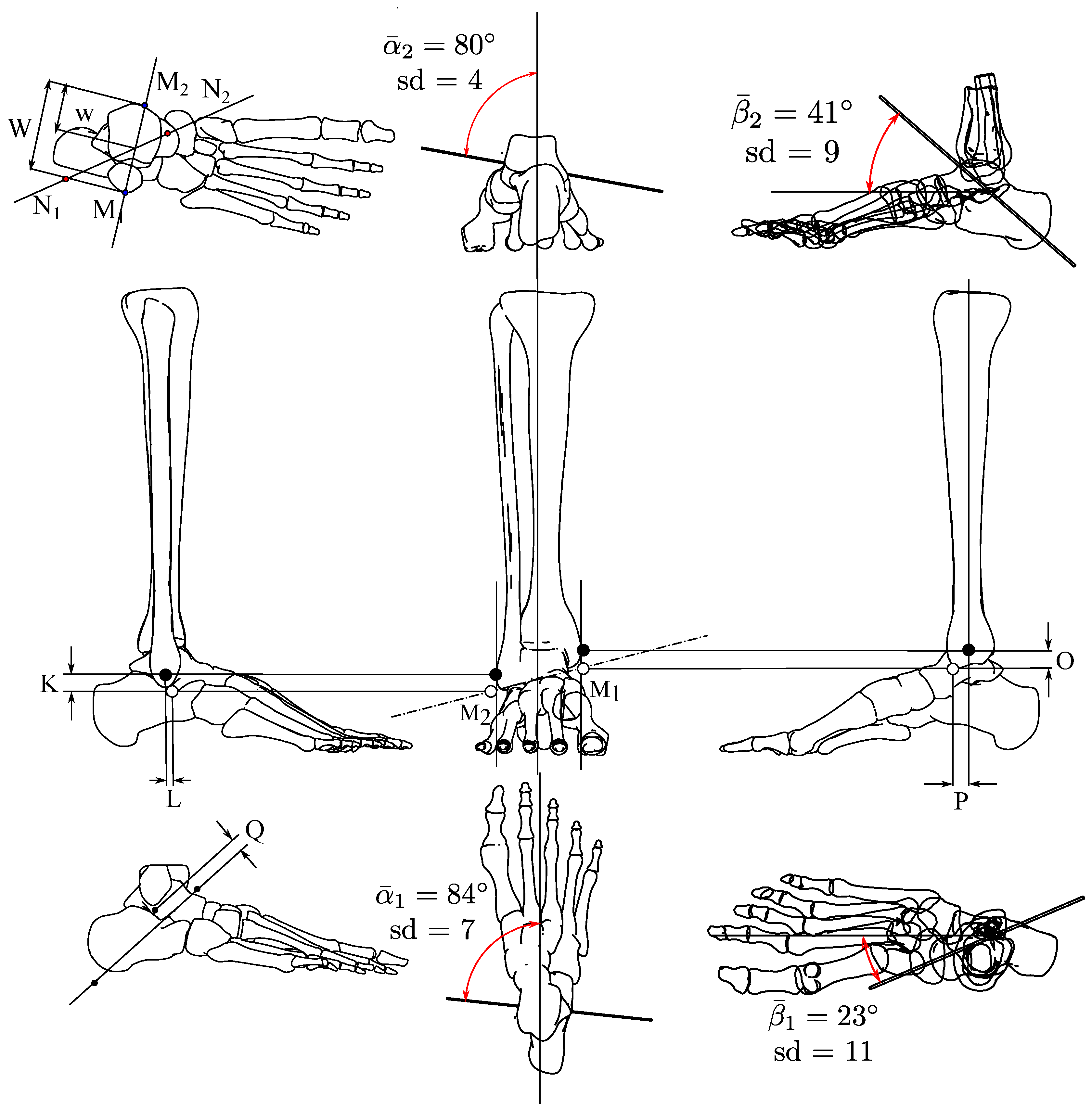
For obtaining the ankle joint model, we use data from anthropometric studies. The values of K, L, O, P, Q with W, and w ratio with standard deviation are in Table A1.

Table A1.
Mean anthropometric values.
| Variable | K (mm) | L (mm) | O (mm) | P (mm) | Q (mm) | R = W/w |
|---|---|---|---|---|---|---|
| Mean value | 12 | 16 | 11 | -1 | 5 | 0.54 |
We show the graphical representation in Figure A1. The figure shows the malleolus most lateral point (MLP), and malleolus mos medial point (MMP). The other values are Q, W and w. , pertain to the talocalcaneal axis; and to the subtalar axis.
The vectors representing the talocrural and talocalcaneal axis can be reflected about the plane y=0 by using the following equation.
Where is the unitary column vector:
yielding
which have the matrix representation:
Replacing the unitary vector , the resulting reflection matrix is:
Then, by multiplying all the right ankle axis vectors by this matrix, we get the left foot kinematic model.
Figure A1.
Ankle anthropometric data.
Appendix A.2. Synthetic Trajectories Generation
In case of the talocrural axis estimation, the trajectories are by plantarflexion and dorsiflexion movements. This means that by blocking the subtalar mobility, the exponential factor will be constant or zero, regarding the initial position election. Assuming the product of exponential formula yields:
Which is a single parameter equation. It corresponds to a circle in the space. We generate the trajectory in the range . We also generate artificial trajectories for the subtalar axis, this is done by replacing the angle , and evaluating for . Then we get:
Appendix A.3. Platform Position
The schematic model is in the Figure A2. It has three base triangles and three attaching points to the foot’s platform. For each point, A, B, and C, we compute the localization in the same way.
Figure A2.
Capturing the platform position.
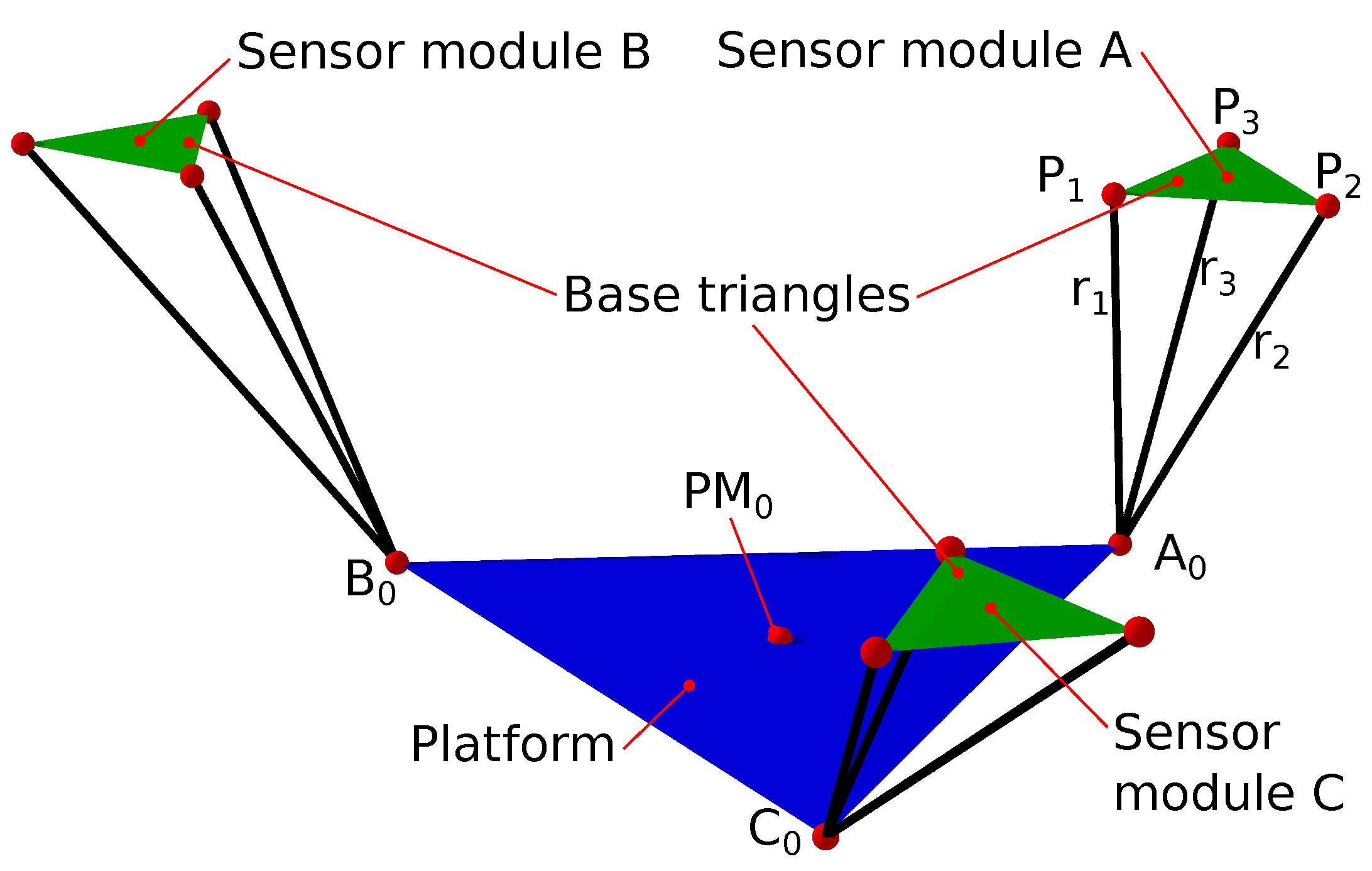
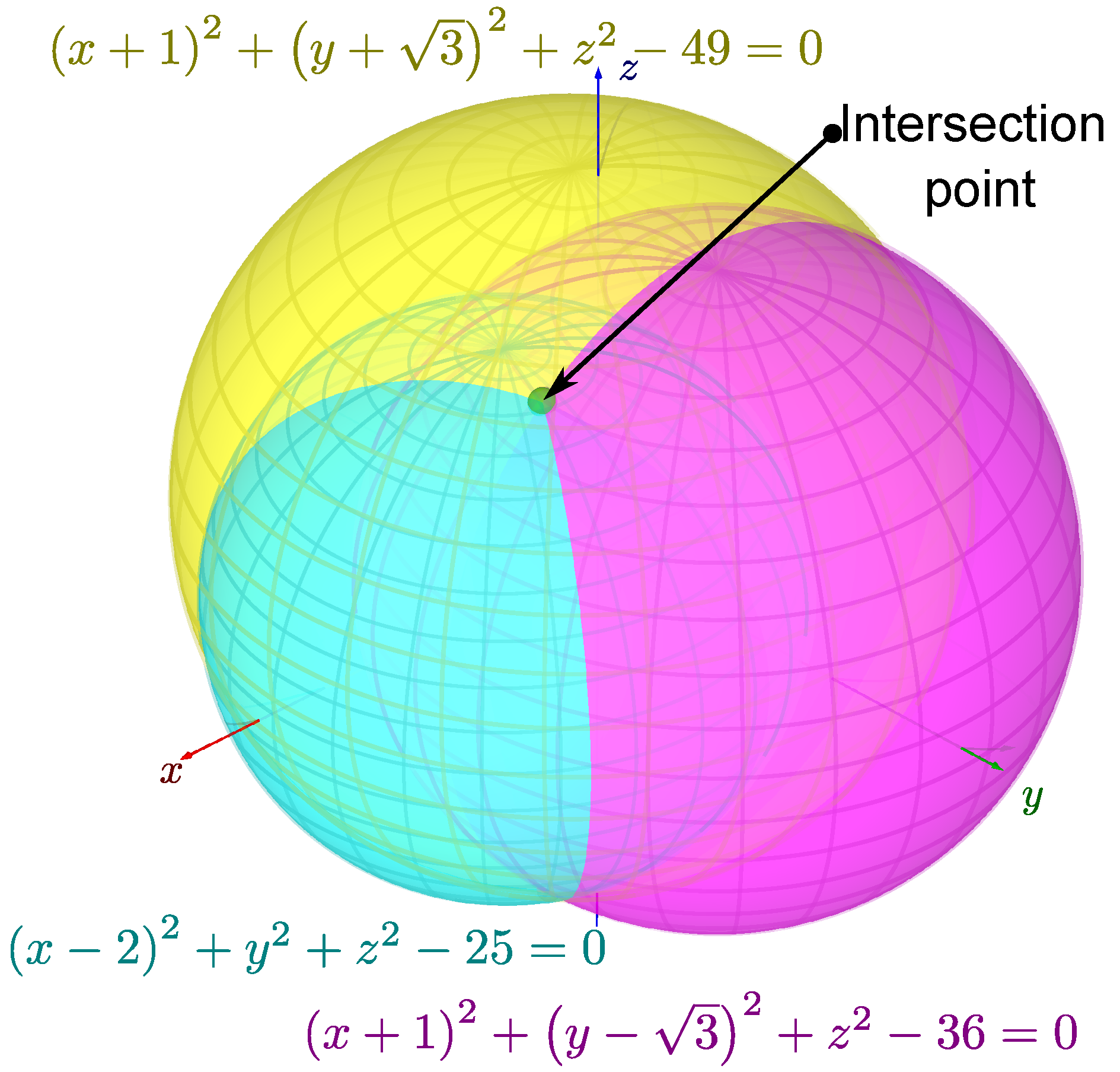
In the figure, we represented three spheres with centers A, B, and C on the plane . Also, we represented the distances , , and measured by each sensor. We translated each equilateral triangle to the origin, then, the vertexes are , , and . Where is the radius from each module center to his vertexes. The sphere’s radius in each module are , , and , then the equations are:
By subtracting the sphere equations from , from , and from , we get the planes:
Which are all parallel to z-axis. Adding and we have the plane:
Solving y in the plane , we get:
And solving for x in plane , we get:
Finally, replacing x and y in , and solving for z, we have:
And solving for x in plane , we get:
In the Figure A3, we show an example when , , , and
Figure A3.
Sphere intersection.
We choose the z-negative value because the origin is over the sensors positions. The Figure A4 shows the geometric representation of the analytic equations.
Figure A4.
Equations’ geometric representation
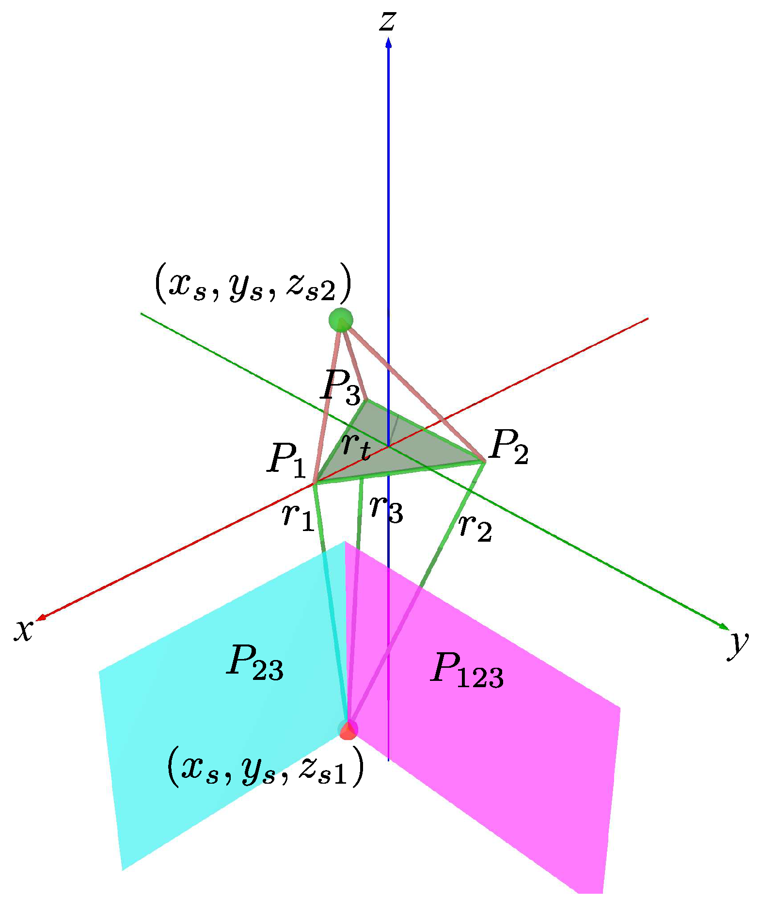
Finally, we translate the origin to A, B, an C center points at the sensor modules.
Appendix A.4. Selecting the Best Circle-Fitting Trajectories
In this subsection, we select the best measured trajectory. We use draw-wire sensors (DWS). The foot position and orientation can be found from the draw-wire sensors by computing vectors from the measured points , , and .
The normal unitary vector is:
A unitary vector pointing forward the foot is:
And a perpendicular vector to and is:
Then, for each instantaneous position we have a measured transformation matrix:
We add two inertial measurement units (IMU), one in the platform and the other in the base. In our design, we use the module GY-6500 with the Invensense’s MPU-6500 chip, which integrates a 3-axis gyroscope, a 3-axis accelerometer and a digital motion processor (DMP). These units have to be first calibrated in a flat surface with the platform coordinates system aligned to the base coordinate’s system. The condition for start and finish a measured trajectory is done by comparing the absolute changes in the accelerometer and the gyroscope.
In the real world, we have noise, and the change must be greater than the noise signal. The noise can be estimated during calibration and measuring absolute maximum and minimum values with the accelerometer and the gyroscope in static positions. We subtract the foot and shank measured quaternions:
And converted the data to angle-axis representation with:
For example, we use measurements in A to get a set of points.
For each point, there are a corresponding IMU attitude:
Then, the mean of the vector list is perpendicular to the plane containing the circular trajectory.
Appendix A.5. Axes Approximation
In this subsection, we used artificial data generated from the anthropometric studies, as an approximation based on real measurements. But the real data will be obtained by using the last subsection method. We briefly describe the method for axis estimation from a selected trajectory containing positions in space. The point positions pertain to a plane with the equation:
Multiplying this equation by , :
If we define:
Then, we have:
solving for z on the right side:
The list of the n sample points has the form:
We define:
Then, the system:
has the solution:
Then, the system:
where:
Is the pseudo-inverse of .
Then we have solved a, b, and d. We replace ,and solve for A, B and D in Equations (A36), (A37), and (A38). In the Equation (A34), the vector is perpendicular to the plane , normalizing the vector, we have:
The angle with the plane , normal to the vector is given by the dot product equation:
the cross product:
is perpendicular to and .
Rotating all the points an angle about the direction vector can be achieved by applying the rotation transformation to each point in the arc:
Where:
And:
Now the points are in a plane parallel to the plane , then we use the two-dimensional circle equation:
Expanding the equation yields:
Rearranging:
Expanding the equation yields:
Which has the form:
Where:
The set of points can be arranged in the system:
Has the form:
Which is similar to the Equation (A45). We found the vector, we found the center and the radius replacing the components in Equations (A58), (A59) and (A60). Then, we rotate back the center using the negative angle , and the same axis . We have three generated trajectories by tracking A, B, and C. Then, we averaged the resulting vectors and centers.
We apply a similar method for the subtalar axis joint. Finally, the initial axis representation is in Plücker line coordinates.
Appendix A.6. Range of Motion
With the axis estimation from a selected trajectory, we compute the corresponding angles for the different positions. The measured homogeneous transformation matrix in the Equation (A.4) measured rotation matrix.
by using the definition of logarithm matrix, we compute the rotation angles as follows. We take the measured trajectories , , and to compute the vectors , , and to get the rotation matrix for each set of measurements. For each trajectory set , , with index i=1 to n measurements. The estimate the angle from the initial position is:
Where is the trace of the measured matrix . In this equation, the angles must be positive, then we choose two groups of measurements. In the set of computed angles, the zero value divides the table in negative and positive values, we defined and , as the negative and positive group of angles. The first group is from the zero position to the maximum value in the negative rotation regarding the rotation axis. The negative maximum angle from the initial position is:
The positive maximum angle from the initial position is:
The range of movement (Rom) is the difference between the positive and the negative value.
This procedure has the same results when we add the two greatest values. We validate the data from the measured rotation matrix, with the skew-symmetric matrix:
With the selected trajectories, we prove that the angle identification is correct.
Appendix A.7. Common Perpendicular and its Feet
The lines representing the axes contain two points and , which are the feet of the common perpendicular line between the axes. We use the Plücker line coordinates to find the intersection points with the axis. Then, we represent the lines with six-dimensional vectors:
The common perpendicular components are:
We compute the intersection points between the common perpendicular and the axes with:
Finally, we have the initial position of the two axes. We use the transverse planes perpendicular to the total tension force in the shank-ankle-foot kinematic chain. For select a central point for the attaching points configuration, we found the projection of each axis on the base plane. It is the result of multiplying the orthogonal projection matrix on the base by :
Also, we project the vectors, , , and . The resulting projections define two lines, we define two points pertaining to the talocrural axis in homogeneous representation:
And for the subtalar axis:
With . Then by using determinants the intersection point components are:
Where:
And:
The reference frames on the base and the platform are are related to the ankle kinematic chain reference frames and by:
We get values for , , , , , and . The kinematic chain, start from , followed by a hinge joint at , then a perpendicular segment to a hinge joint at , ending in the platform center . In summary, we obtained a simplified model for the shank-ankle-foot kinematic chain.
Appendix B. Synthetic Data for Validation.
Appendix B.1. Ankle Forward Kinematics.
There are two reference systems, the base with origin and the platform, with origin at the platform center. The initial points are in Table A2.
Table A2.
Platform’s initial position.
| Platform radius | Origin distance | Initial Point | Initial Point | Initial Point |
|---|---|---|---|---|
| 11.57 | 17.62 | (-11.57, 0.0000, -17.62) | (5.785, 10.02, -17.62) | (5.785, -10.02, -17.62) |
* units in cm.
The point is the mean value from , , and . The mean values from the sample anthropometric measurements the resulting values for , , are in Table A3.
Table A3.
Talocrural axis approximation.
| Foot width | |||
|---|---|---|---|
| 96.42 | (0,0,-107.81) | (5.359, -50.99, -116.9) | (-4.565, 43.44, -100.1) |
1 units in mm.
And, for , , are in Table A4.
Table A4.
Subtalar axis approximation.
| Foot length | |||
|---|---|---|---|
| 266.5 | (3.2803, 0, -111.58) | (-95.07, -27.70, -197.1) | (101.6, 27.70, -26.09) |
1 units in mm.
In this context, we have the points , , and pertaining to the talocrural axis. Also, , , and pertain to the subtalar axis. We used the mean values for , , , from Table A5.
Table A5.
Mean values for the axis attitude.
| Angle Identifier | Mean (sexagesimal) |
|---|---|
The resulting vectors for the product of exponentials matrix representation are in Table A6.
Table A6.
Vectors for the product of exponentials matrices.
| Axis and point | ||
|---|---|---|
| Talocrural on | (-0.103, 0.979, 0.174) | (106., 11.1, 0) |
| Subtalar on | 0.738, 0.208, 0.642) | (23.2, -84.5, 0.682) |
The components of the rotation matrix are:
The components of the translation vector for A reference point are:
The group of movements for the point A are given by.
Where the rotation matrix is:
And the translation vector is:
With the range of movement for , and , we get the group of movements for each vertex on the platform. We also apply the same transformation to the group of movements for B, C, and .
We change the talocrural and subtalar axes attitude from the Table A7.
Table A7.
Ankle axes attitude modifications.
| Angle Identifier | Maximum | Minimum |
|---|---|---|
We show the resulting and values in the Table A8.
Table A8.
Direction vectors of the ankle axes.
| Group of values | ||
|---|---|---|
| Maximum | (0.0174, 0.994, 0.105) | (0.629, 0.208, 0.749) |
| Minimum | (-0.218, 0.945, 0.242) | (0.703, 0.559, 0.439) |
The resulting and are in Table A9.
Table A9.
Momentum for maximum and minimum axis attitude.
| Group of values | ||
|---|---|---|
| Maximum | (107., -1.87, 0) | (23.1, -72.7, 0.796) |
| Minimum | (102., 23.5, 0) | (62.7, -79.9, 1.48) |
We also show the data generated from reflection matrix, resulting in artificial data for the left foot. The resulting reflection matrix about the sagittal plane is:
The resulting reflected platform initial points are in Table A10.
Table A10.
Left foot platform initial points.
| left | left | left |
|---|---|---|
| (-115.7, 0, -176.18) | (57.849, 100.20, -176.18) | (57.849, -100.20, -176.18) |
The talocrural reflected points are in Table A11.
Table A11.
Talocrural axis reflected points.
| reflected | reflected |
|---|---|
| (5.3595, 50.992, -116.85) | (-4.5655, -43.438, -100.11) |
And for the subtalar axis the resulting reflected points are in Table A12.
Table A12.
Subtalar axis reflected points.
| reflected | reflected |
|---|---|
| (-95.071, 27.700, -197.08) | (101.63, -27.700, -26.088) |
Appendix B.2. Axes’ Common Perpendicular and Feet Points.
After characterizing the axes and its range of motion, we compute the common perpendicular line and the intersection points (feet) with the estimated axes. The feet points will be used for represent the shank-foot-ankle kinematic chain. In this subsection, we use the results from Table A6, Table A8, and Table A9. We compute the common perpendicular from the minimum, maximum and mean axis attitude from the Table A13.
Table A13.
Axes’ vectors for minimum, mean and maximum values.
| Axis attitude | ||||
|---|---|---|---|---|
| Minimum | (-0.218, 0.945, 0.242) | (102, 23.5, 0) | (0.703, 0.559, 0.439) | (62.7, -79.9, 1.48) |
| Mean | (-0.103, 0.979, 0.174) | (106., 11.1, 0) | (0.738, 0.208, 0.642) | (23.2, -84.5, 0.682) |
| Maximum | (0.0174, 0.994, 0.105) | (107, -1.87, 0) | (0.629, 0.208, 0.749) | (23.1, -72.7, 0.796) |
For each group of values, the resulting common perpendicular and feet are in Table A14.
Table A14.
Common perpendicular and feet points.
| Axis attitude | ||||
|---|---|---|---|---|
| Minimum | (0.2796, 0.2658, -0.7862) | (26, -30, -2.4) | (-0.94, 4.1, -110) | (-32, -26, -19) |
| Mean | (0.5923, 0.1945, -0.7439) | (20, -64, -2.2) | (-0.24, 2.3, -110) | (-51, -14, -44) |
| Maximum | (0.7227, 0.05301, -0.6216) | (15, -79, 9.2) | (-0.24, -14, -110) | (-54, -18, -63) |
Now, we have almost three different configurations, only by changing the axes’ attitude statistical values.
Appendix B.3. Subtalar Axis Range of Motion.
The range of motion for the subtalar axis is similar to the talocrural, the points for the negative angles are in the Table A15.
Table A15.
Subtalar axis negative angles points.
| Sample set i | Trajectory A | Trajectory B | Trajectory C |
|---|---|---|---|
| 1 | (-111.42 6.5037 -183.21) | (42.270 -118.34 -152.38) | (76.602 75.518 -189.75) |
| 2 | (-112.41 5.3489 -181.69) | (45.794 -115.24 -157.44) | (73.062 81.010 -187.46) |
| 3 | (-113.34 4.1020 -180.21) | (49.150 -111.81 -162.41) | (69.365 86.283 -184.92) |
| 4 | (-114.22 2.7668 -178.78) | (52.329 -108.09 -167.27) | (65.520 91.322 -182.13) |
| 5 | (-115.03 1.3469 -177.39) | (55.322 -104.06 -172.02) | (661.539 96.111 -179.10) |
The points difference in this case is on the Table A16.
Table A16.
Points differences for the subtalar negative angles.
| Sample set i | ||
|---|---|---|
| 1 | (153.69 -124.85 30.829) | (188.02 69.014 -6.5481) |
| 2 | (158.20 -120.59 24.255) | (185.47 75.661 -5.7695) |
| 3 | (162.49 -115.92 17.808) | (182.71 82.181 -4.7012) |
| 4 | (166.54 -110.85 11.507) | (179.74 88.555 -3.3472) |
| 5 | (170.35 -105.41 5.3694) | (176.56 94.764 -1.7107) |
The components for the rotation matrices in this case are in the Table A17.
Table A17.
Rotation matrices components for the subtalar axis negative angles.
| Sample set i | Vector | Vector | Vector |
|---|---|---|---|
| 1 | (-0.0377 0.196 0.980) | (0.984 -0.161 0.0700) | (0.171 0.967 -0.187) |
| 2 | (-0.0328 0.156 0.987) | (0.990 -0.129 0.0533) | (0.136 0.979 -0.150) |
| 3 | (-0.0264 0.116 0.993) | (0.995 -0.0972 0.0378) | (0.101 0.989 -0.112) |
| 4 | (-0.0186 0.0755 0.997) | (0.998 -0.0642 0.0235) | (0.0658 0.995 -0.0741) |
| 5 | (-0.00945 0.0356 0.999) | (0.999 -0.0307 0.0105) | (0.0310 0.999 -0.03534) |
The rotation matrices for the subtalar axis negative angles are in the Table A18.
Table A18.
Subtalar axis negative angles rotation matrices.
| Sample set i | Rotation matrix | Angle (Rad) | Angle (Deg) |
|---|---|---|---|
| 1 | 0.26181 | 15.001 | |
| 2 | 0.20838 | 11.939 | |
| 3 | 0.15495 | 8.8777 | |
| 4 | 0.10153 | 5.8173 | |
| 5 | 0.048085 | 2.7551 |
The greatest of the negative angles is . The Table A19 shows the points for the subtalar positive angles.
Table A19.
Subtalar axis positive angles trajectories.
| Sample set i | Trajectory A | Trajectory B | Trajectory C |
|---|---|---|---|
| 1 | (-116.32 -1.4090 -175.01) | (60.212 -96.112 -180.22) | (54.066 104.06 -173.08) |
| 2 | (-116.94 -3.0434 -173.76) | (62.640 -91.324 -184.56) | (49.766 108.08 -169.43) |
| 3 | (-117.49 -4.7460 -172.58) | (64.851 -86.289 -188.74) | (45.374 111.81 -165.59) |
| 4 | (-117.97 -6.5117 -171.46) | (66.840 -81.021 -192.73) | (40.903 115.23 -161.55) |
| 5 | (-118.37 -8.3355 -170.40) | (68.602 -75.534 -196.54) | (36.366 118.33 -157.34) |
The points differences are in the Table A20.
Table A20.
Points difference for the subtalar axis positive angles.
| Sample set i | ||
|---|---|---|
| 1 | (176.53 -94.703 -5.2102) | (170.38 105.47 1.9314) |
| 2 | (179.58 -88.281 -10.798) | (166.70 111.13 4.3313) |
| 3 | (182.34 -81.543 -16.158) | (162.86 116.55 6.9919) |
| 4 | (184.81 -74.509 -21.276) | (158.87 121.74 9.9048) |
| 5 | (186.97 -67.199 -26.137) | (154.74 126.66 13.062) |
The rotation matrices components are in the Table A21.
Table A21.
Components of the rotation matrices for the subtalar axis positive angles.
| Sample set i | Vector | Vector | Vector |
|---|---|---|---|
| 1 | (0.0105 -0.0353 0.999) | (0.999 0.0310 -0.00945) | (-0.0307 0.999 0.0356) |
| 2 | (0.0235 -0.0741 0.997) | (0.998 0.0658 -0.0186) | (-0.0642 0.995 0.07553) |
| 3 | (0.0378 -0.112 0.993) | (0.995 0.101 -0.0264) | (-0.0972 0.989 0.116) |
| 4 | (0.0533 -0.150 0.987) | (0.990 0.136 -0.0328) | (-0.129 0.979 0.156) |
| 5 | (0.0700 -0.187 0.980) | (0.984 0.171 -0.0377) | (-0.161 0.967 0.196) |
The rotation matrices for the subtalar axis positive angles are in Table A22.
Table A22.
Rotation matrices for the subtalar axis positive angles.
| Sample set i | Rotation matrix | Angle (Rad) | Angle (Deg) |
|---|---|---|---|
| 1 | 0.048085 | 2.7551 | |
| 2 | 0.10153 | 5.8173 | |
| 3 | 0.15495 | 8.8777 | |
| 4 | 0.20838 | 11.939 | |
| 5 | 0.26180 | 15.000 |
The greatest positive value is . Then the range of motion is .
References
- Parre, M.D.; Sujatha, B. Novel Human-Centered Robotics: Towards an Automated Process for Neurorehabilitation. 2021, 6690715. [CrossRef]
- Ziefle, M.; Schaar, A.K. Technology Acceptance by Patients: Empowerment and Stigma. [CrossRef]
- Pinheiro, C.; Figueiredo, J.; Magalhães, N.; Santos, C.P. Wearable Biofeedback Improves Human-Robot Compliance during Ankle-Foot Exoskeleton-Assisted Gait Training: A Pre-Post Controlled Study in Healthy Participants. 20, 5876. Number: 20 Publisher: Multidisciplinary Digital Publishing Institute. [CrossRef]
- Fischer, D.K.B.; Kristiansen, J.; Mariager, C.S.; Frendrup, J.; Rehm, M. People-Centered Development of a Smart Learning Ecosystem of Adaptive Robots. In The Interplay of Data, Technology, Place and People for Smart Learning; Springer. [CrossRef]
- He, W.; Li, Z.; Chen, C.P. A survey of human-centered intelligent robots: issues and challenges. 4, 602–609. Publisher: IEEE.
- Zhou, L.; Li, Y.; Bai, S. A human-centered design optimization approach for robotic exoskeletons through biomechanical simulation. 91, 337–347. Publisher: Elsevier.
- Schmidtler, J.; Knott, V.; Hölzel, C.; Bengler, K. Human centered assistance applications for the working environment of the future. 12, 83–95. Publisher: IOS Press.
- Misgeld, B.J.E.; Gerlach-Hahn, K.; Rüschen, D.; Pomprapa, A.; Leonhardt, S. Control of Adjustable Compliant Actuators. 2, 134–157. [CrossRef]
- Wade, E.; Winstein, C.J. Virtual reality and robotics for stroke rehabilitation: where do we go from here? 18, 685–700. [CrossRef]
- Yang, R.; Ji, L.; Chen, H. Novel Human-Centered Rehabilitation Robot with Biofeedback for Training and Assessment. In Proceedings of the Universal Access in Human-Computer Interaction. Applications and Services; Stephanidis, C., Ed. Springer, Lecture Notes in Computer Science, pp. 472–478. [CrossRef]
- Riener, R.; Lünenburger, L.; Colombo, G. Human-centered robotics applied to gait training and assessment. 43.
- Miao, Q.; Zhang, M.; Wang, C.; Li, H. Towards Optimal Platform-Based Robot Design for Ankle Rehabilitation: The State of the Art and Future Prospects. 2018, e1534247. Publisher: Hindawi. [CrossRef]
- Dong, M.; Zhou, Y.; Li, J.; Rong, X.; Fan, W.; Zhou, X.; Kong, Y. State of the art in parallel ankle rehabilitation robot: a systematic review. 18, 52. [CrossRef]
- Jahanyani, A.; Matloub, S.K.; Matloub, R.K.; Zahraei, S.A.H. Robot-Assisted Therapy on Ankle Rehabilitation, A Mini Review. 36, 28796–28797. Company: Biomedres Distributor: Biomedres Institution: Biomedres Label: Biomedres Publisher: Biomedical Research Network+, LLC. [CrossRef]
- Hussain, S.; Jamwal, P.K.; Vliet, P.V.; Brown, N.A.T. Robot Assisted Ankle Neuro-Rehabilitation: State of the art and Future Challenges. 21, 111–121. Publisher: Taylor & Francis _eprint: https://doi.org/10.1080/14737175.2021.1847646. [CrossRef]
- Khalid, Y.M.; Gouwanda, D.; Parasuraman, S. A review on the mechanical design elements of ankle rehabilitation robot. 229, 452–463. Publisher: IMECHE. [CrossRef]
- Alvarez-Perez, M.G.; Garcia-Murillo, M.A.; Cervantes-Sánchez, J.J. Robot-assisted ankle rehabilitation: a review. 15, 394–408. Publisher: Taylor & Francis _eprint: https://doi.org/10.1080/17483107.2019.1578424. [CrossRef]
- Chin, L.C.e.; Basah, S.N.; Affandi, M.; Shah, M.N.; Yaacob, S.; Juan, Y.E.; Din, M.Y. Home-Based Ankle Rehabilitation system: Literature Review and Evaluation. 79. Number: 6. [CrossRef]
- Jiang, J.; Lee, K.M.; Ji, J. Review of anatomy-based ankle–foot robotics for mind, motor and motion recovery following stroke: design considerations and needs. 2, 267–282. [CrossRef]
- Liu, Z.; Lu, D. Research Progress of Lower Limb Rehabilitation Robots in Mainland China. 7, 92–105. [CrossRef]
- Briot, S.; Bonev, I. Are Parallel Robots More Accurate than Serial Robots? 31, 445–455. [CrossRef]
- Liao, Z.; Yao, L.; Lu, Z.; Zhang, J. Screw theory based mathematical modeling and kinematic analysis of a novel ankle rehabilitation robot with a constrained 3-PSP mechanism topology. 2, 351–360. [CrossRef]
- Li, Q.; Huang, Z. Mobility analysis of lower-mobility parallel manipulators based on screw theory. In Proceedings of the 2003 IEEE International Conference on Robotics and Automation (Cat. No.03CH37422), Vol. 1, pp. 1179–1184 vol.1. ISSN: 1050-4729. [CrossRef]
- Lynch, K.M.; Park, F.C. Modern Robotics: Mechanics, Planning, and Control; Cambridge University Press. Google-Books-ID: OB4xDwAAQBAJ.
- Mueller, A. Modern Robotics: Mechanics, Planning, and Control [Bookshelf]. 39, 100–102. [CrossRef]
- Gosselin, C. Cable-driven parallel mechanisms: state of the art and perspectives. 1, DSM0004–DSM0004. [CrossRef]
- Zarebidoki, M.; Dhupia, J.S.; Xu, W. A Review of Cable-Driven Parallel Robots: Typical Configurations, Analysis Techniques, and Control Methods. 29, 89–106. [CrossRef]
- Pott, A. Cable-Driven Parallel Robots: Theory and Application; Springer. Google-Books-ID: eH1TDwAAQBAJ.
- Zhang, Z.; Shao, Z.; You, Z.; Tang, X.; Zi, B.; Yang, G.; Gosselin, C.; Caro, S. State-of-the-art on theories and applications of cable-driven parallel robots. 17, 37. [CrossRef]
- Dežman, M.; Asfour, T.; Ude, A.; Gams, A. Mechanical design and friction modelling of a cable-driven upper-limb exoskeleton. 171, 104746. [CrossRef]
- Wei, W.; Qu, Z.; Wang, W.; Zhang, P.; Hao, F. Design on the Bowden Cable-Driven Upper Limb Soft Exoskeleton. 2018, 1925694. [CrossRef]
- Sales Gonçalves, R.; Carvalho, J.; Rodrigues, L.A.; Marques Barbosa, A. Cable-Driven Parallel Manipulator for Lower Limb Rehabilitation; Vol. 459. [CrossRef]
- Erdogan, A.; Celebi, B.; Satici, A.C.; Patoglu, V. AssistOn-Ankle: a reconfigurable ankle exoskeleton with series-elastic actuation. 41, 743–758. [CrossRef]
- Yu, R.; Fang, Y.; Guo, S. Design and kinematic performance analysis of a cable-driven parallel mechanism for ankle rehabilitation. 37, 53–62 and 73. [CrossRef]
- Russo, M.; Ceccarelli, M. Analysis of a Wearable Robotic System for Ankle Rehabilitation. 8, 48. [CrossRef]
- Ozawa, R.; Kobayashi, H.; Hashirii, K. Analysis, Classification, and Design of Tendon-Driven Mechanisms. 30, 396–410. [CrossRef]
- Ravella, K.C.; Ahmad, J.; Amirouche, F. Biomechanics of the Ankle Joint; Springer International Publishing; pp. 401–413. [CrossRef]
- Wu, G.; Siegler, S.; Allard, P.; Kirtley, C.; Leardini, A.; Rosenbaum, D.; Whittle, M.; D’Lima, D.D.; Cristofolini, L.; Witte, H.; et al. ISB recommendation on definitions of joint coordinate system of various joints for the reporting of human joint motion–part I: ankle, hip, and spine. International Society of Biomechanics. 35, 543–548. [CrossRef]
- Okubo, K.; Kervyn, G.; Zielinski, M.; Vinent, L.; Bigio, A.T.; Villar., C.T. Open Source Anatomy. https://www.z-anatomy.com, accessed on 2023-05-29.
- The Sage Developers. SageMath, the Sage Mathematics Software System (Version 10.0), 2023. https://www.sagemath.org.
- Vargas-Riaño, J.H. Turmell-Bot - nbviewer. https://nbviewer.org/github/juliohvr/Turmell-Bot/blob/main/TurmellBot.ipynb, accessed on 2023-06-17.
- Vargas-Riaño, J.H. Turmell-Bot | 3D CAD Model Library | GrabCAD. https://grabcad.com/library/turmell-bot-1, accessed on 2023-06-17.
- Vargas-Riaño, J.H. juliohvr/Turmell-Bot: Turmell-Bot. https://github.com/juliohvr/Turmell-Bot. [CrossRef]
- Isman, R.E.; Inman, V.T. Anthropometric Studies of the Human Foot and Ankle; Biomechanics Laboratory, University of California. Google-Books-ID: 4Xq0GwAACAAJ.
- Drillis, R.; Contini, R.; New York University.; School of Engineering and Science. Body segment parameters; New York University, School of Engineering and Science. OCLC: 22352502.
- Fryar, C.D.; Carroll, M.D.; Gu, Q.; Afful, J.; Ogden, C.L. Anthropometric Reference Data for Children and Adults: United States, 2015-2018. pp. 1–44.
- Agudelo-Varela, Ó.; Vargas-Riaño, J.; Valera, Á. Turmell-Meter: A Device for Estimating the Subtalar and Talocrural Axes of the Human Ankle Joint by Applying the Product of Exponentials Formula. 9, 199. [CrossRef]
- Todorov, E.; Erez, T.; Tassa, Y. MuJoCo: A physics engine for model-based control. In Proceedings of the 2012 IEEE/RSJ International Conference on Intelligent Robots and Systems. IEEE, 2012, pp. 5026–5033. [CrossRef]
- Zhao, J.; Li, B.; Yang, X.; Yu, H. Geometrical method to determine the reciprocal screws and applications to parallel manipulators. 27, 929–940. [CrossRef]
Figure 1.
Lateral top and medial bottom views of the ankle-foot anatomy. (a) Lateral top view with components tangential to each axis. (b) Medial bottom view with components tangential to each axis [39].
Figure 1.
Lateral top and medial bottom views of the ankle-foot anatomy. (a) Lateral top view with components tangential to each axis. (b) Medial bottom view with components tangential to each axis [39].
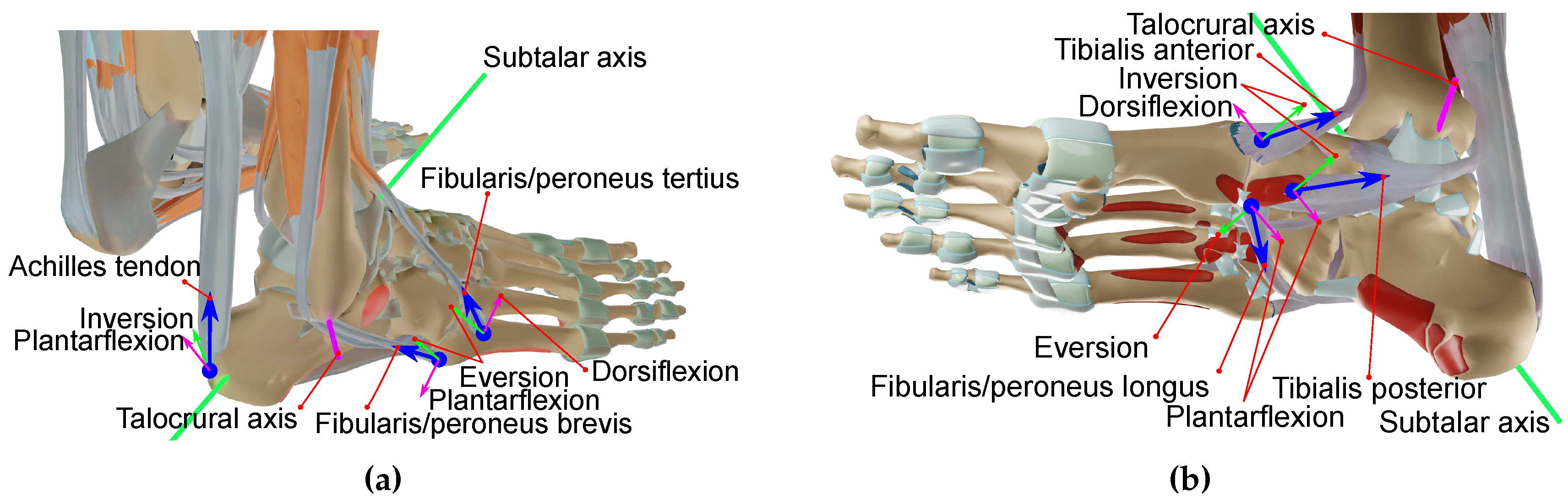
Figure 2.
Right foot’s bottom plantar plane projection with contact points and joint axis.
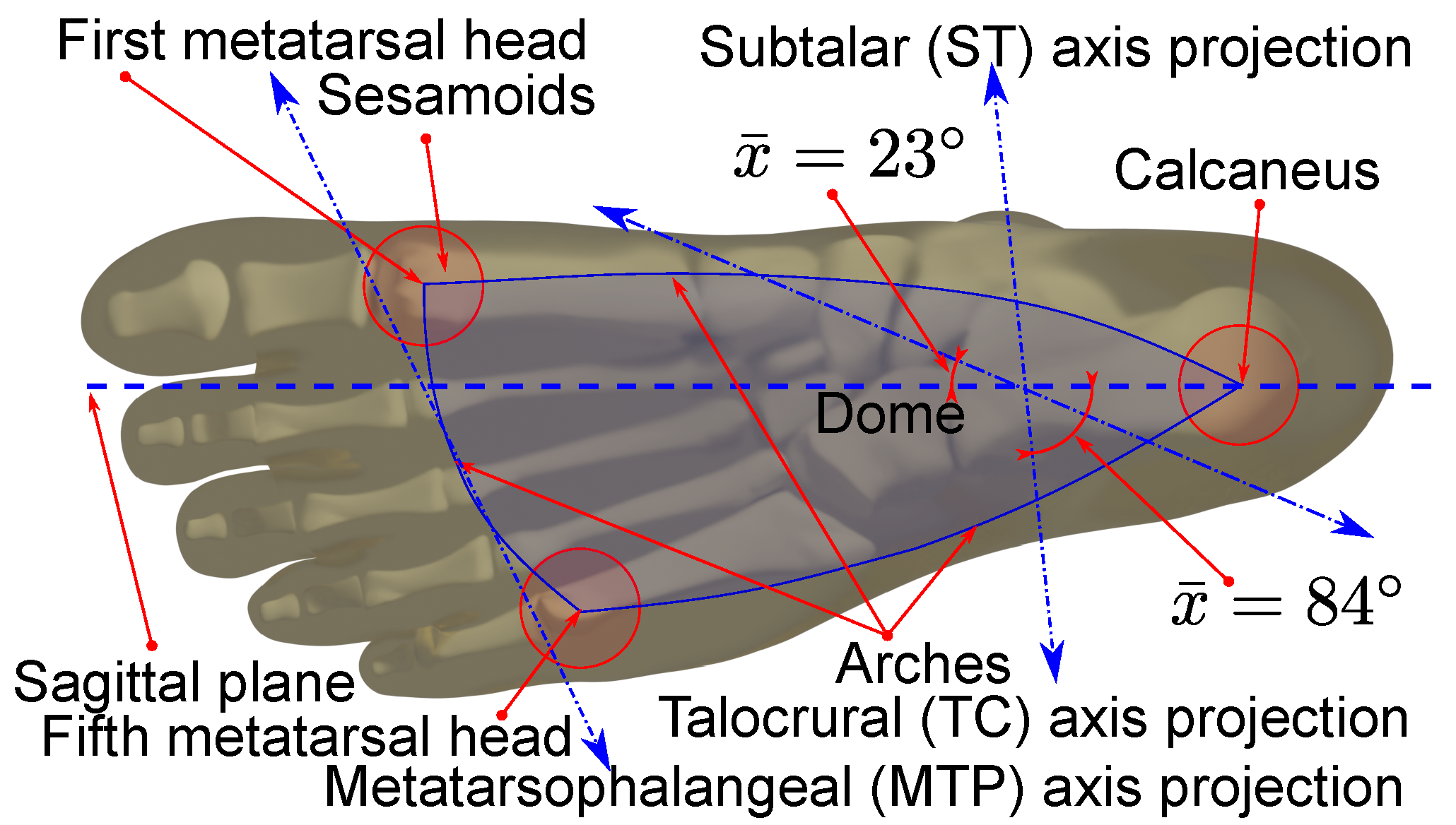
Figure 3.
Ankle model and ankle rehabilitation robot sketch. (a) Schematic representation of the approximated tendon directions in neutral position. (b) Schematic representation of reconfiguration.
Figure 3.
Ankle model and ankle rehabilitation robot sketch. (a) Schematic representation of the approximated tendon directions in neutral position. (b) Schematic representation of reconfiguration.
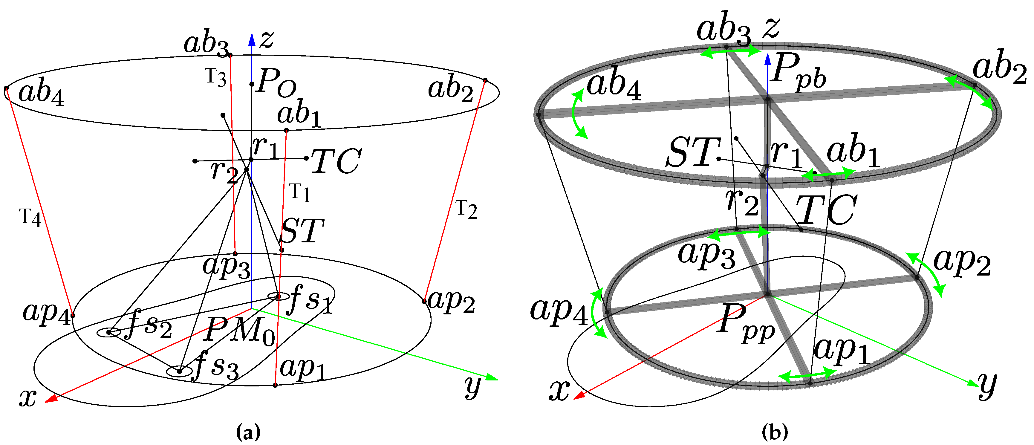
Figure 4.
Size design from proportions and statistics. (a) Proportions. (b) Three dimensional simplified design.
Figure 4.
Size design from proportions and statistics. (a) Proportions. (b) Three dimensional simplified design.
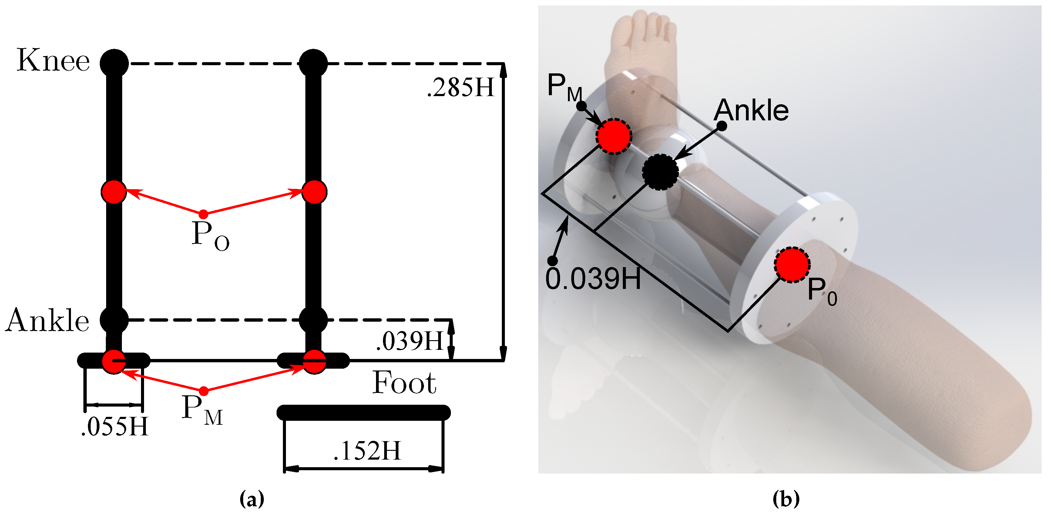
Figure 5.
Product of exponentials representation of the ankle joint [47].
Figure 5.
Product of exponentials representation of the ankle joint [47].
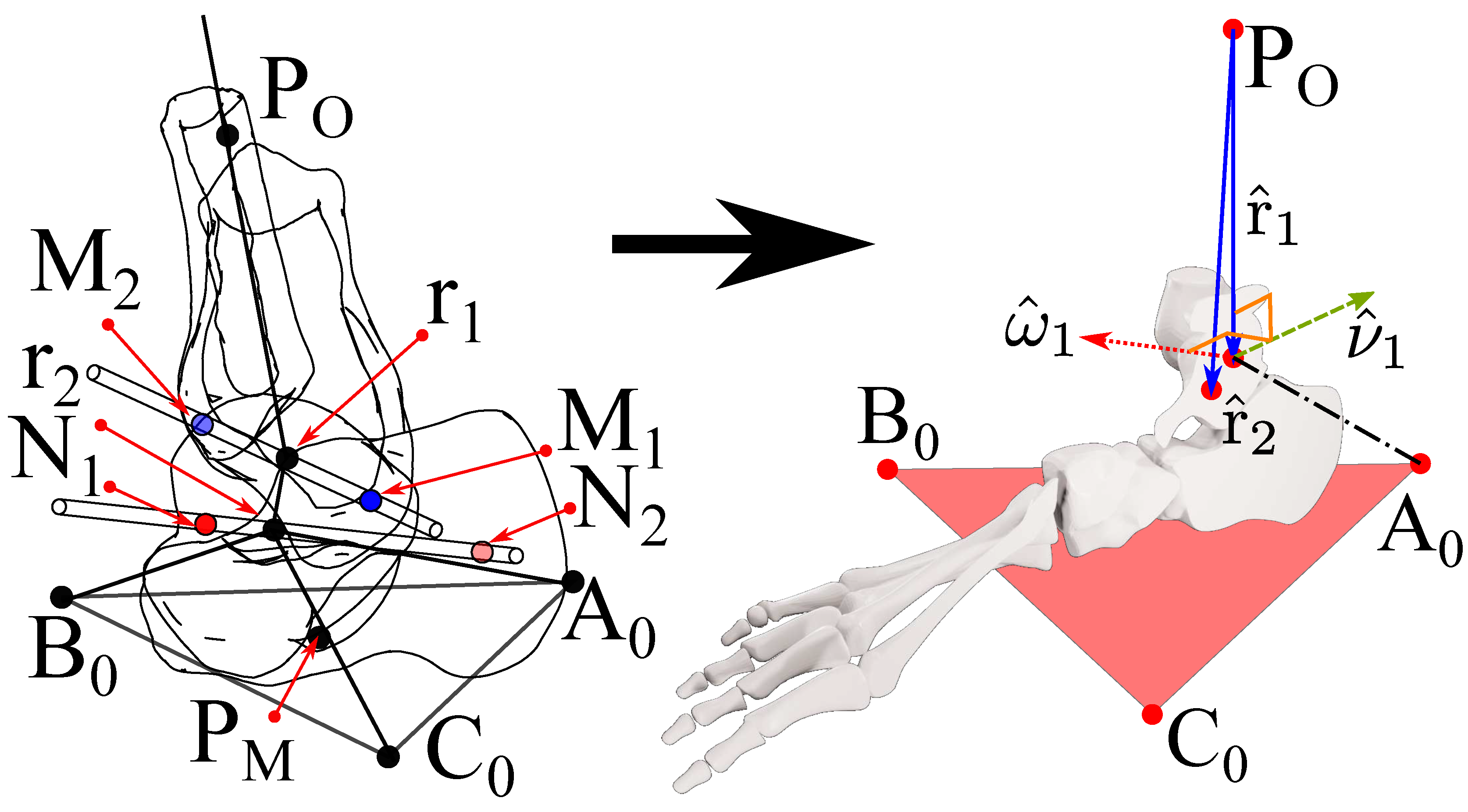
Figure 6.
Base and platform sizes initial approximation. (a) Leg coronal section. (b) Collision, range of motion, and antagonistic actuation.
Figure 6.
Base and platform sizes initial approximation. (a) Leg coronal section. (b) Collision, range of motion, and antagonistic actuation.
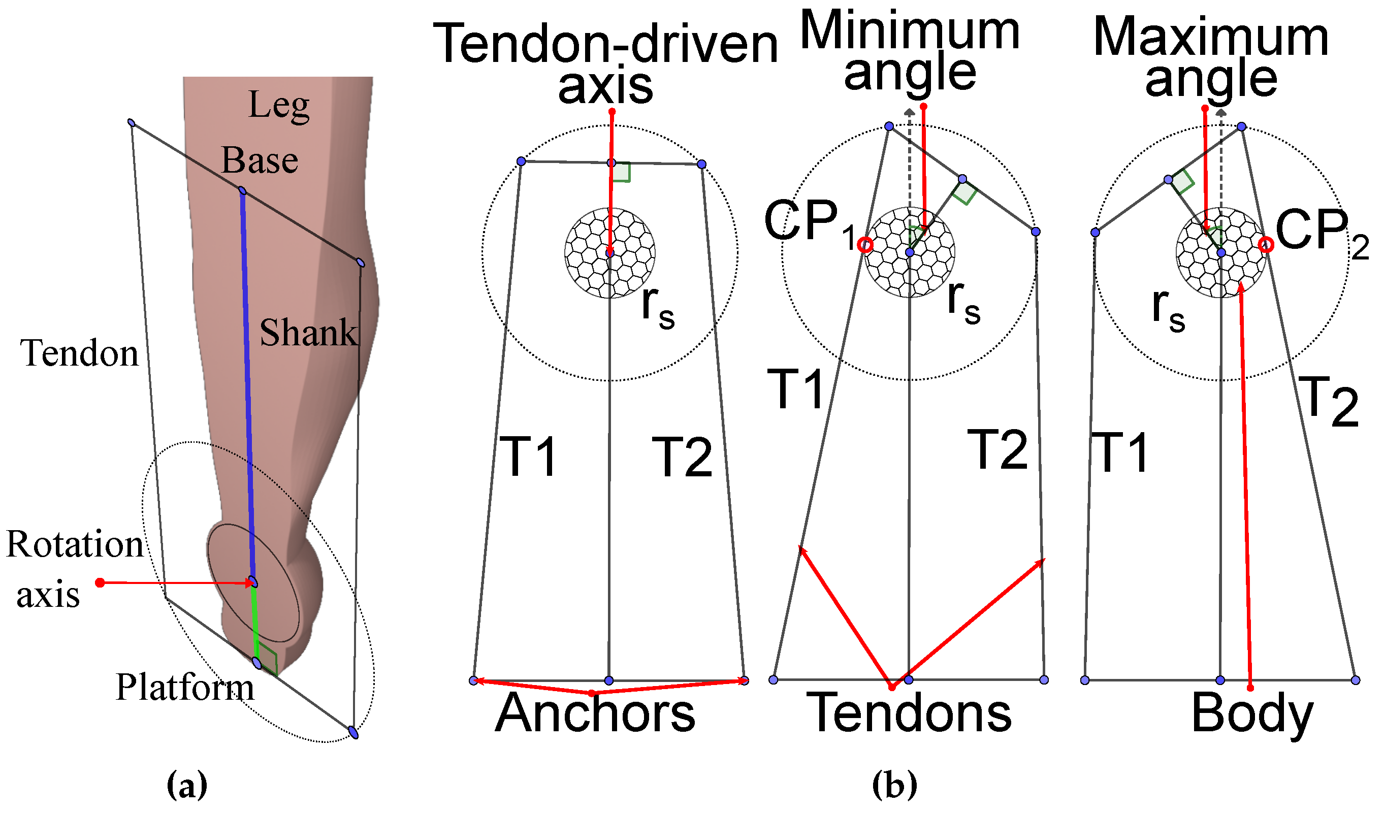
Figure 7.
Maximum displacement.
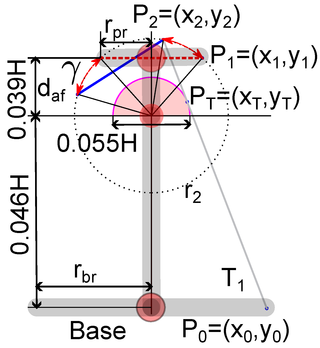
Figure 8.
Normal views of the proximal and distal axis regarding the base. (a) Normal view to the proximal axis. (b) Normal view to the distal axis.
Figure 8.
Normal views of the proximal and distal axis regarding the base. (a) Normal view to the proximal axis. (b) Normal view to the distal axis.
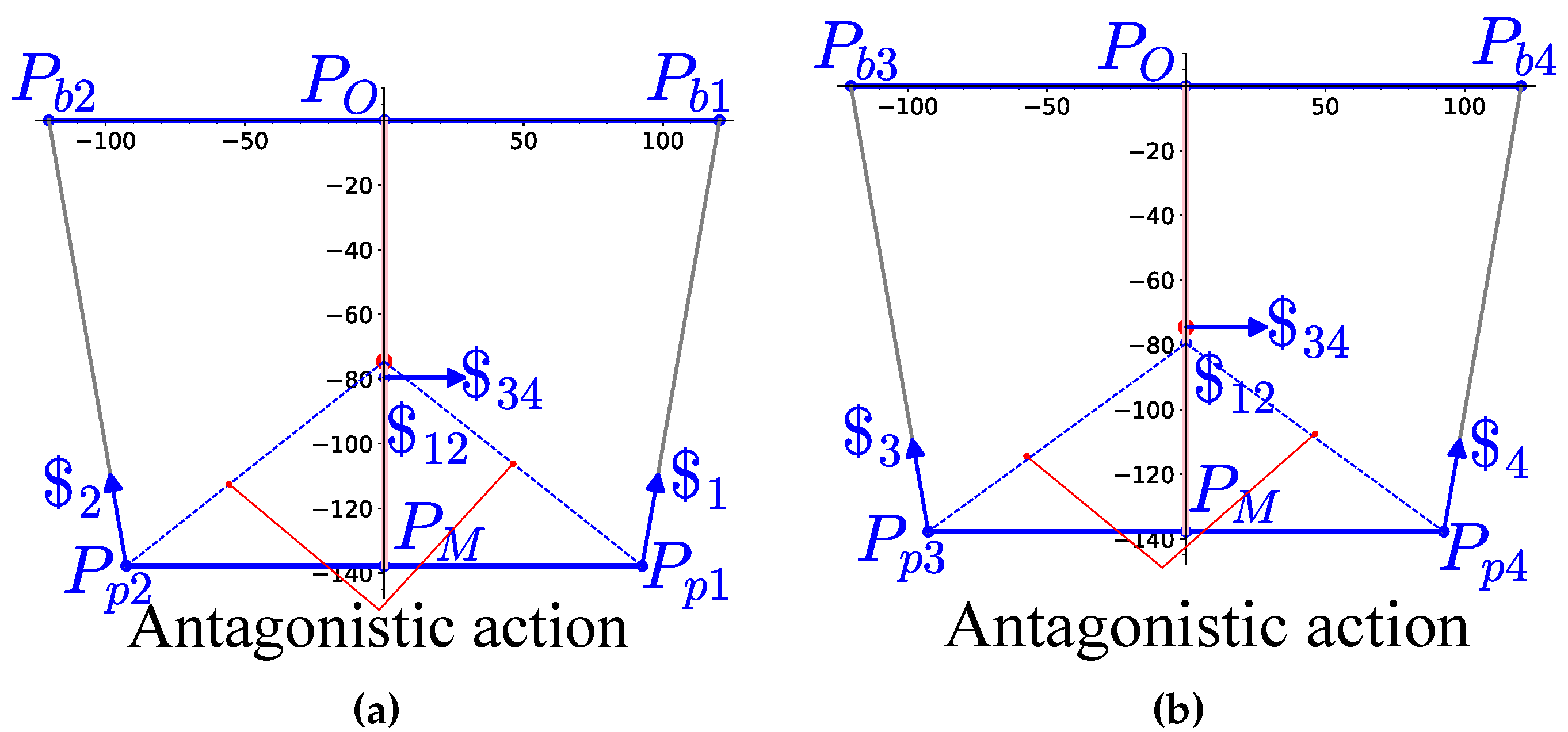
Figure 9.
First approximation with orthogonal axis coplanar to the tendons. (a) Antagonistic cables screws representation. (b) Screw representation for the anchor points rotated .
Figure 9.
First approximation with orthogonal axis coplanar to the tendons. (a) Antagonistic cables screws representation. (b) Screw representation for the anchor points rotated .
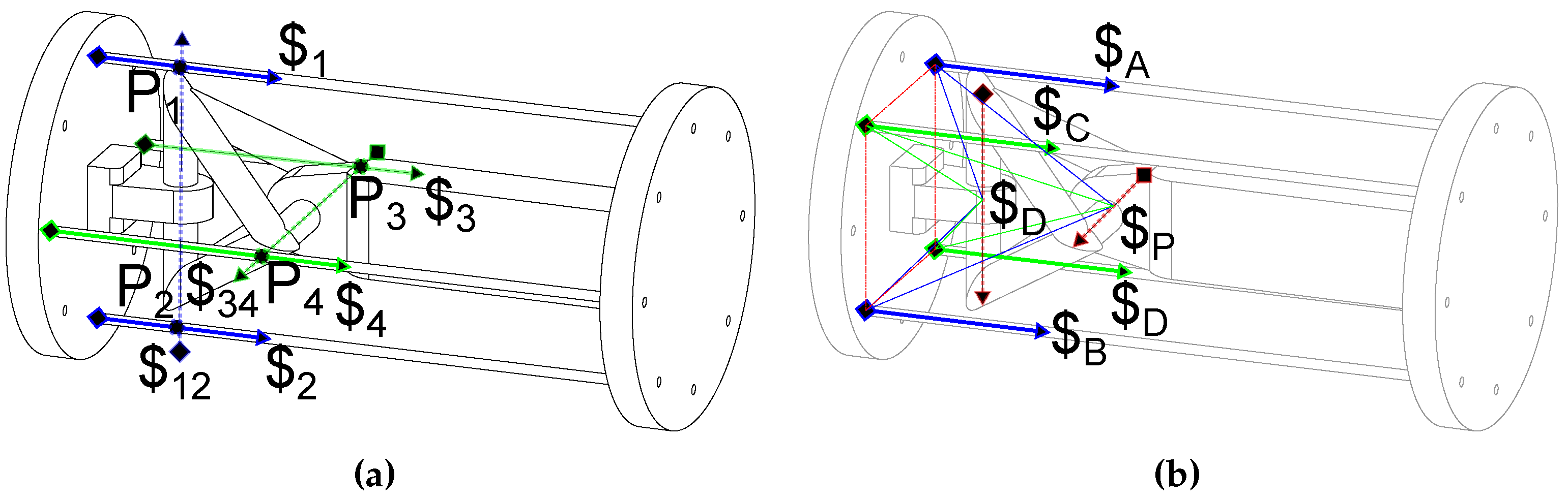
Figure 10.
Range of motion and platform-base proportions. (a) Mean height. (b) Maximum height. (c) Minimum height.
Figure 10.
Range of motion and platform-base proportions. (a) Mean height. (b) Maximum height. (c) Minimum height.
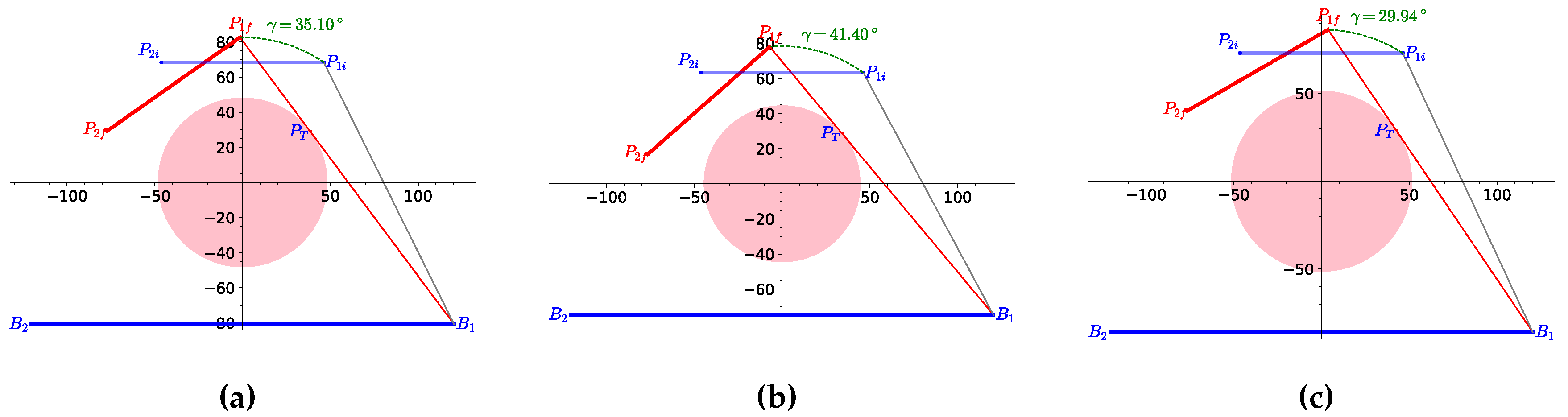
Figure 11.
Anchor points at initial position. (a) Mean statistical attitude. (b) Maximum statistical attitude. (c) Minimum statistical attitude.
Figure 11.
Anchor points at initial position. (a) Mean statistical attitude. (b) Maximum statistical attitude. (c) Minimum statistical attitude.
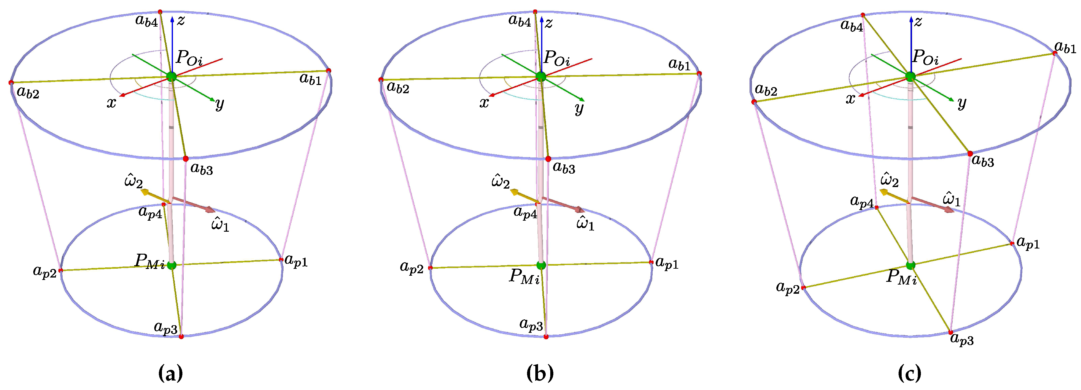
Figure 12.
Robot kinematics. (a) Centering the platform. (b)Forward kinematics.
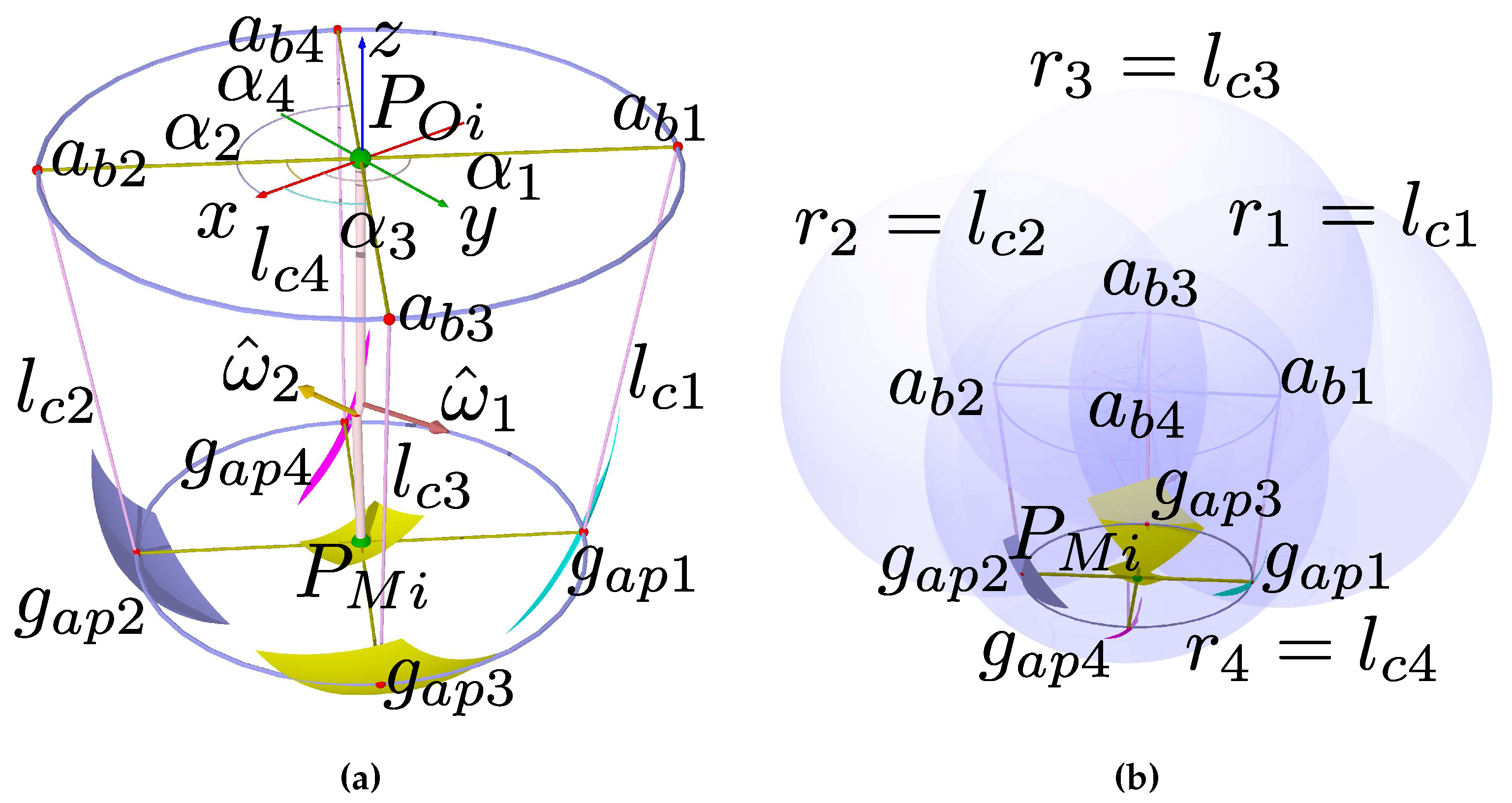
Figure 13.
Configurations for axes’ mean attitude values. a) Minimal TC and ST angles. (b)Minimal TC and ST maximal angles. c) Maximal TC and maximal ST angles. (b) TC and ST maximal angles.
Figure 13.
Configurations for axes’ mean attitude values. a) Minimal TC and ST angles. (b)Minimal TC and ST maximal angles. c) Maximal TC and maximal ST angles. (b) TC and ST maximal angles.
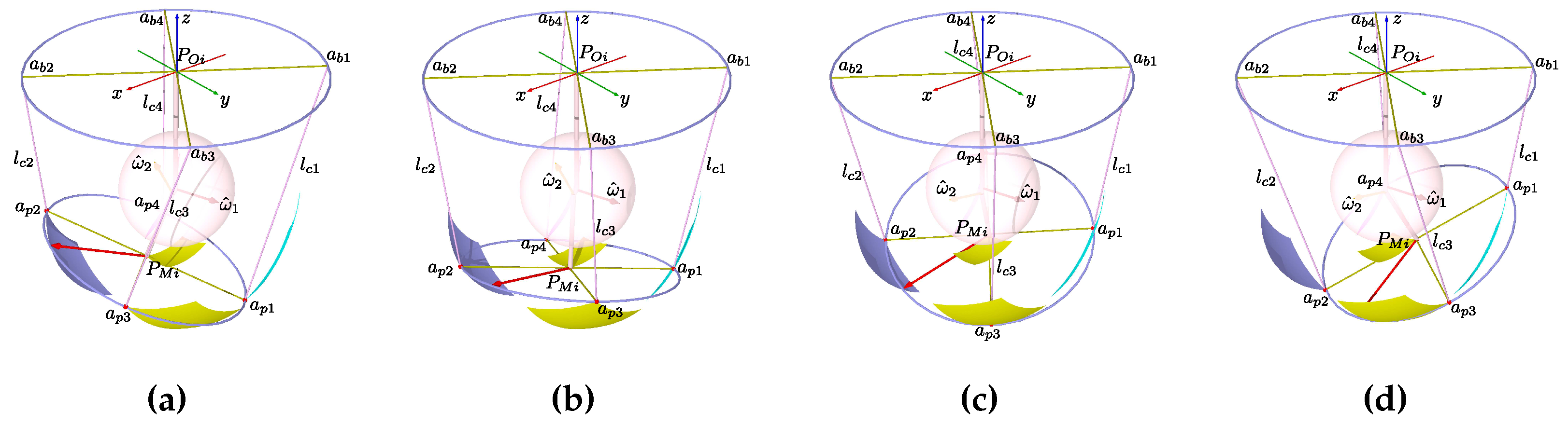
Figure 14.
Configurations corresponding to the axes’ maximum attitude values. a) Minimal TC and ST angles. (b)Minimal TC and ST maximal angles. c) Maximal TC and maximal ST angles. (b) TC and ST maximal angles.
Figure 14.
Configurations corresponding to the axes’ maximum attitude values. a) Minimal TC and ST angles. (b)Minimal TC and ST maximal angles. c) Maximal TC and maximal ST angles. (b) TC and ST maximal angles.
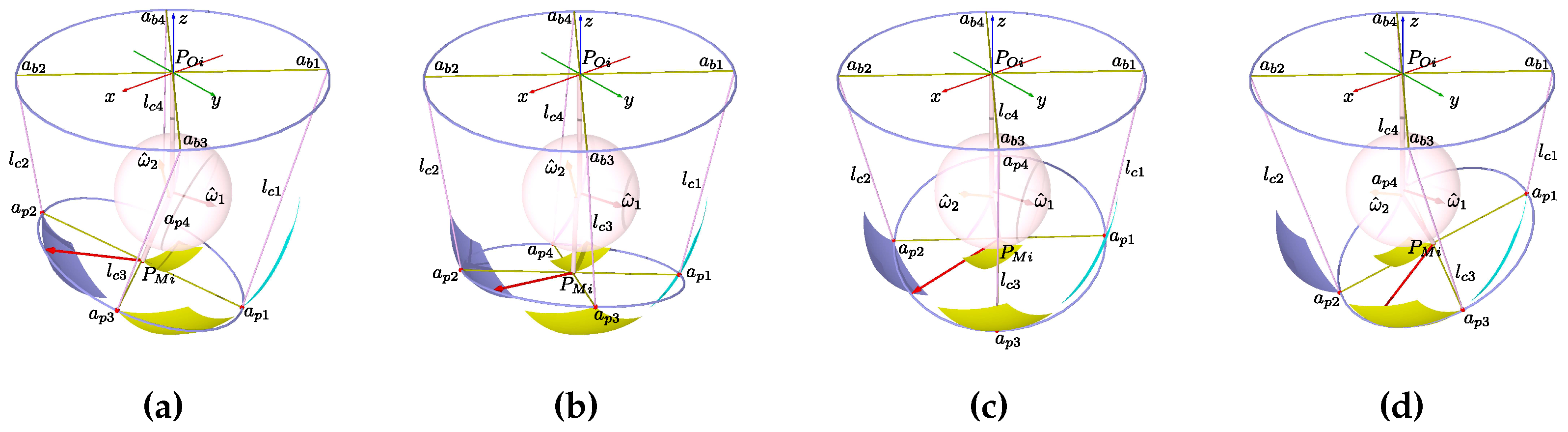
Figure 15.
Configurations for the axes’ minimum attitude values. a) Minimal TC and ST angles. (b)Minimal TC and ST maximal angles. c) Maximal TC and maximal ST angles. (b) TC and ST maximal angles.
Figure 15.
Configurations for the axes’ minimum attitude values. a) Minimal TC and ST angles. (b)Minimal TC and ST maximal angles. c) Maximal TC and maximal ST angles. (b) TC and ST maximal angles.
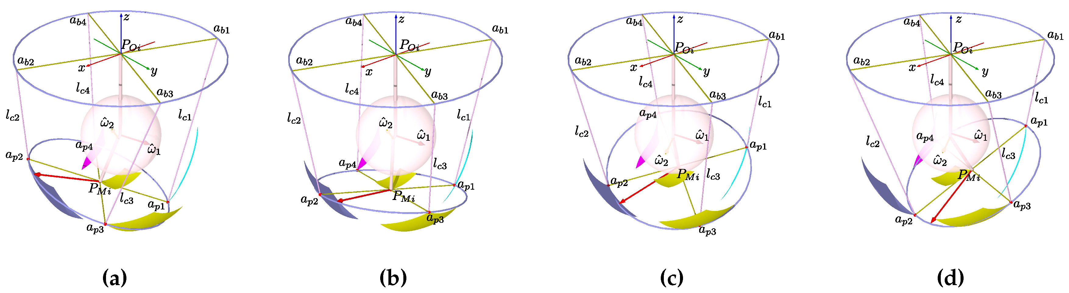
Figure 16.
Simulation at initial position.
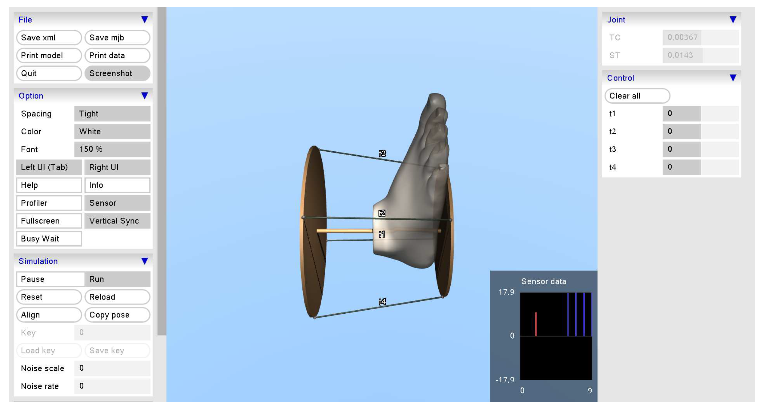
Figure 17.
Snapshots of MuJoCo Simulate with extreme angles configurations. a) Minimal TC and ST angles. (b)Maximal TC and ST minimal angles. c) Minimal TC and maximal ST angles. (b) TC and ST maximal angles.
Figure 17.
Snapshots of MuJoCo Simulate with extreme angles configurations. a) Minimal TC and ST angles. (b)Maximal TC and ST minimal angles. c) Minimal TC and maximal ST angles. (b) TC and ST maximal angles.
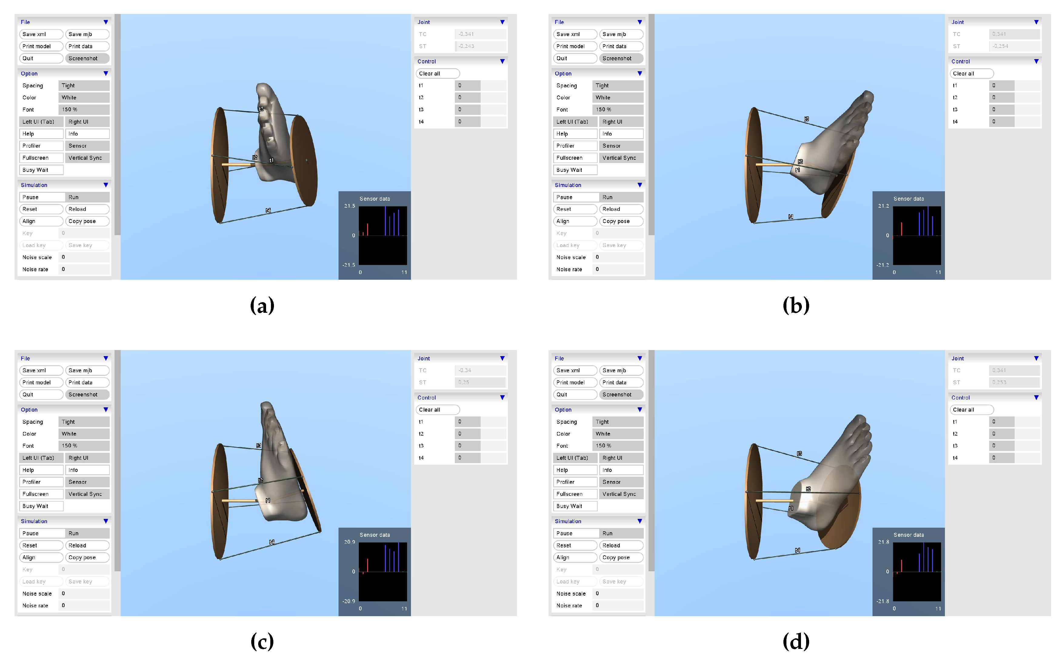
Figure 18.
Foot’s size adjust.
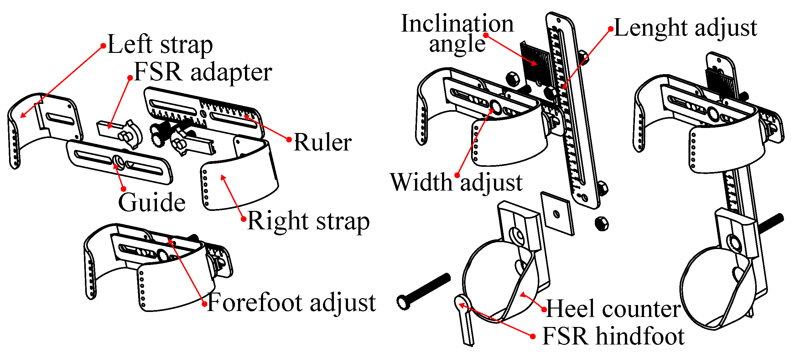
Figure 19.
Centering the platform.
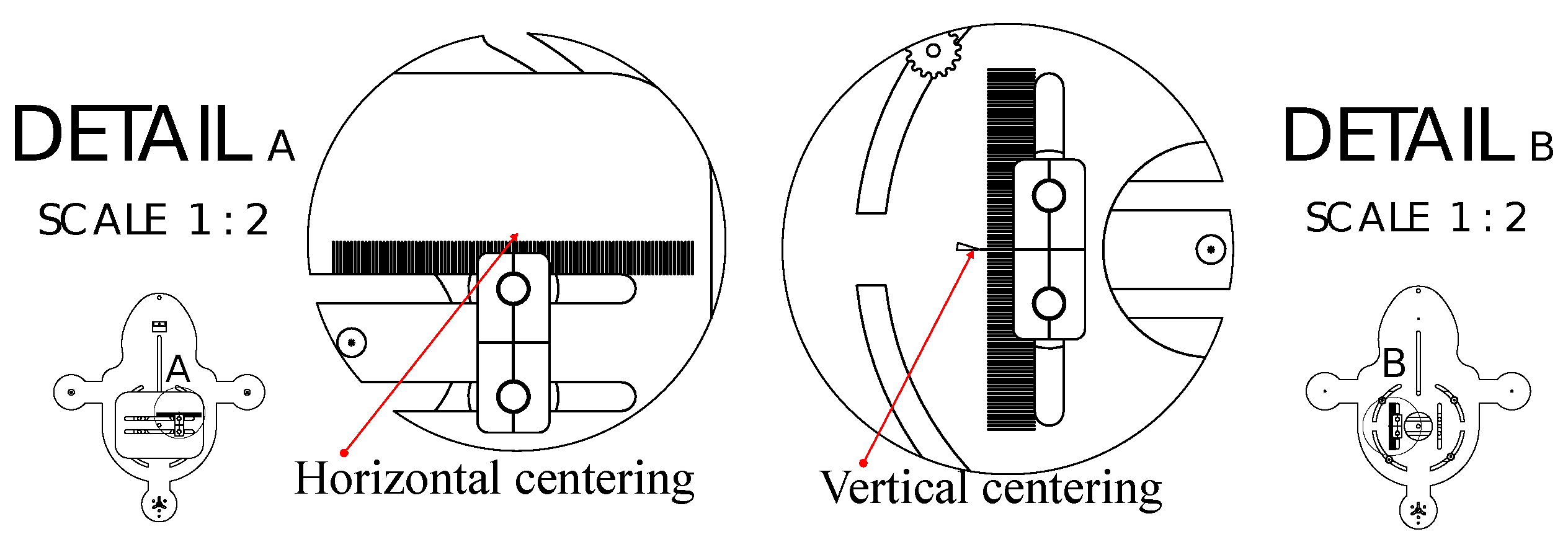
Figure 20.
Centering the base.
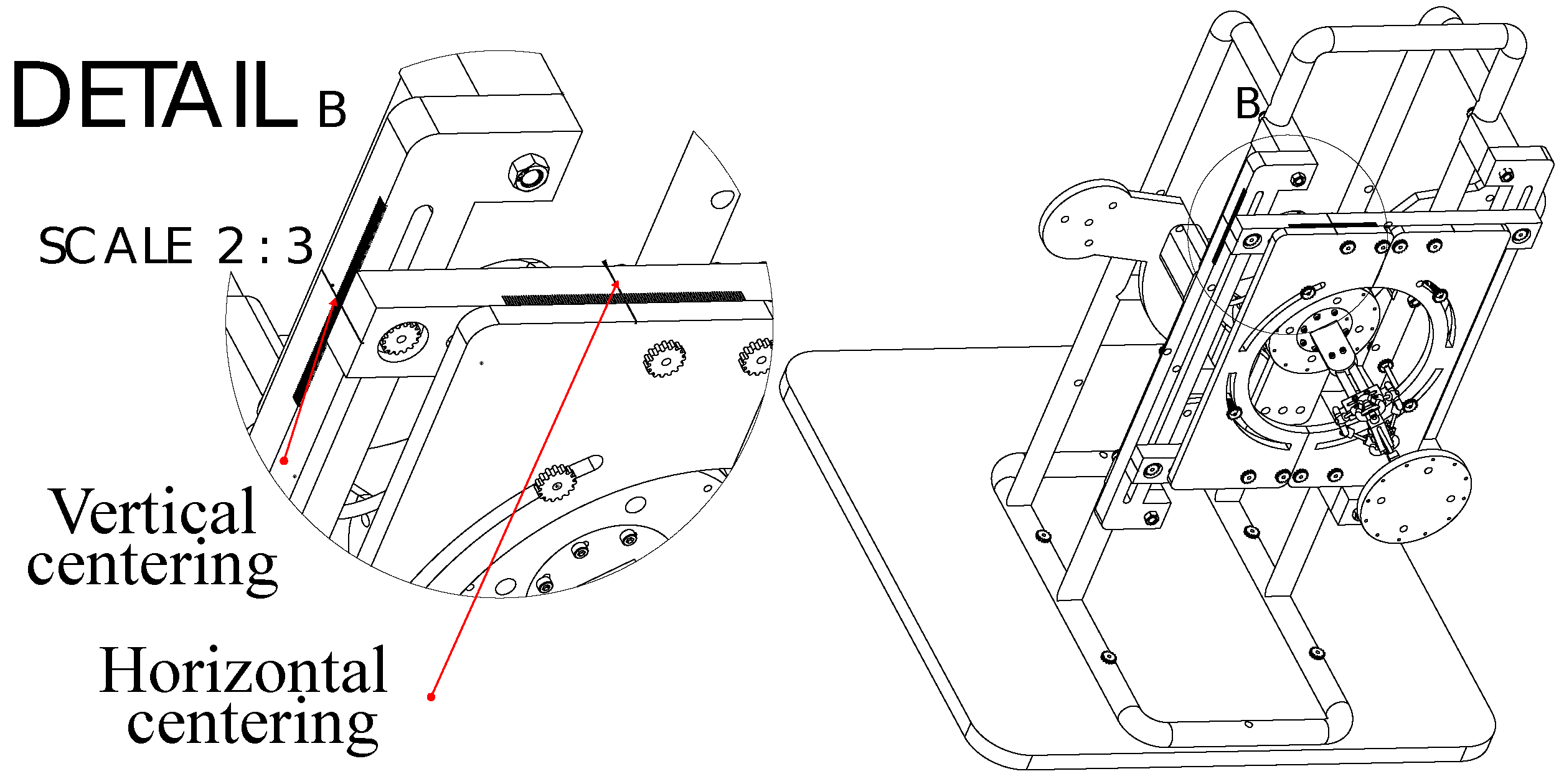
Figure 21.
CAD design.
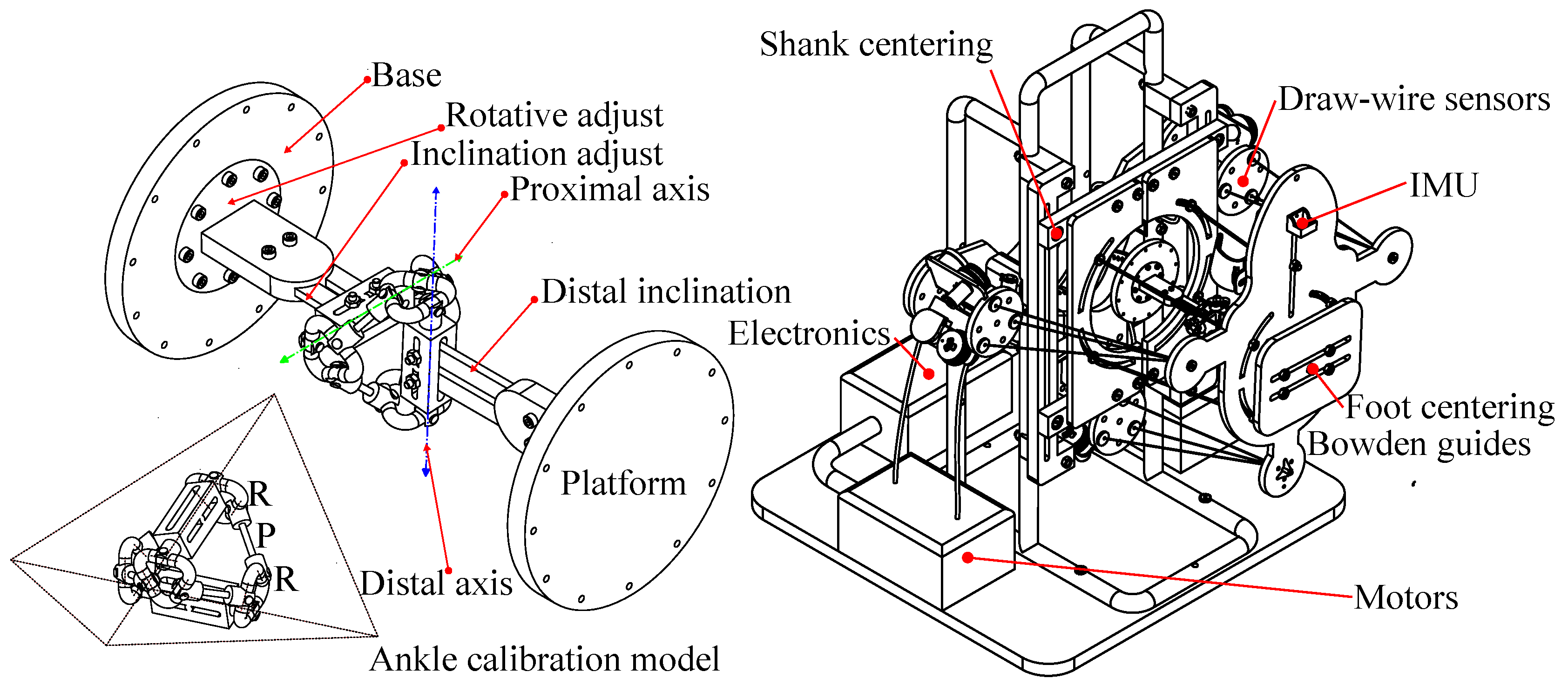
Table 1.
Size radius for the circumscribed triangles for the platform, base, and modules.
| Platform radius | Base radius | Module radius |
|---|---|---|
| 115.698 mm. | 150.4074 mm. | 30 mm. |
Table 2.
Vertex position for a module centered at the origin.
| Sensor | Sensor | Sensor |
|---|---|---|
| (30, 0, 0) | (-15, 25.98, 0) | (-15, -25.98, 0) |
Table 3.
Base reference vertexes.
| Base vertex A | Base vertex B | Base vertex C |
|---|---|---|
| (-150.4, 0, 0) | (75.2, 130.3, 0) | (75.2, -130.3, 0) |
Table 4.
Distances from the initial points to the corresponding sensors.
| Sensor module | Distance to | Distance to | Distance to |
|---|---|---|---|
| A | =176.2 | =184.9 | =184.9 |
| B | =176.2 | =311.1 | =269.9 |
| C | =293.9 | =269.9 | =311.1 |
Table 5.
Platform points computation.
| Point | Original from the model | Estimation from lengths |
|---|---|---|
| (-115.7, 0, -176.18) | (-115.7, -0, -176.18) | |
| (57.849, -100.2, -176.18) | (57.849, -100.2, -176.18) | |
| (57.849, 100.2, -176.18) | (57.849, 100.2, -176.18) |
Table 6.
Normal vector, angle, rotation axis for the talocrural axis estimation.
| Trajectory | Unitary normal vector | Angle (rad) | Talocrural axis direction |
|---|---|---|---|
| A | (-0.10295, 0.97941, 0.17364) | 1.3963 | (0.99452, 0.10453, 0) |
| B | (-0.10293, 0.97942, 0.17364) | 1.3963 | (0.99452, 0.10452, 0) |
| C | (-0.10294, 0.97941, 0.17364) | 1.3963 | (0.99452, 0.10452, 0) |
Table 7.
Circle-fitting for the talocrural axis estimation.
| Trajectory | Center parallel to plane x-y | Radius | Estimated center |
|---|---|---|---|
| A | (-10.76, 105.8, -18.68) | 134.5 | (0.34535, 0.098175, -107.93) |
| B | (-9.798, 106.1, -134.7) | 65.33 | (13.265, -113.37, -128.29) |
| C | (-14.11, 101.6, 61.59) | 111.9 | (-11.603, 77.660, -90.225) |
Table 8.
Talocrural mean rotation axis and center.
| Trajectory estimation | Mean rotation axis | Mean trajectory center |
|---|---|---|
| Talocrural joint | (-0.10294, 0.97941, 0.17364) | (0.66912, -11.871, -108.81) |
Table 9.
Plane containing the trajectories A, B and C for the subtalar axis estimation.
| Trajectory | Unitary normal vector | Angle (rad) | Subtalar Axis |
|---|---|---|---|
| A | (0.73827, 0.20787, 0.64167) | 0.87412 | (0.27102, -0.96257, 0) |
| B | (0.73823, 0.20790, 0.64171) | 0.87407 | (0.27108, -0.96256, 0) |
| C | (0.73821, 0.20789, 0.64174) | 0.87404 | (0.27107, -0.96256, 0) |
Table 10.
Circle-fitting for the subtalar axis estimation.
| Trajectory | Center parallel to plane x-y | Radius | Estimated center |
|---|---|---|---|
| A | (79.45, 26.55, -198.5) | 33.37 | (-95.929, -22.830, -191.53) |
| B | (84.05, 23.25, -91.18) | 129.8 | (-13.335, -4.1798, -125.39) |
| C | (84.50, 22.43, -49.52) | 130.7 | (17.795, 3.6453, -98.822) |
Table 11.
Subtalar mean rotation axis and center.
| Trajectory estimation | Mean rotation axis | Mean trajectory center |
|---|---|---|
| Talocrural joint | (0.73824, 0.20789, 0.64171) | (-30.490, -7.7882, -138.58) |
Table 12.
Axes estimation.
| Axis direction vector | Original | Estimated | Absolute error |
|---|---|---|---|
| (-0.10294, 0.97941, 0.17365) | (-0.10294, 0.97941, 0.17364) | 0.0000081395 | |
| (105.59, 11.098, 0) | (104.51, 11.085, -0.56662) | 1.2164 | |
| (0.73822, 0.20791, 0.64172) | (0.73824, 0.20789, 0.64171) | 0.000035358 | |
| (23.199, -84.478, 0.68201) | (23.811, -82.740, -0.58889) | 2.2381 |
Table 13.
Negative angles group.
| Sample set i | Trajectory A | Trajectory B | Trajectory C |
|---|---|---|---|
| 1 | (-85.819 9.2808 -210.81) | (72.031 -102.03 -157.42) | (82.714 97.870 -148.31) |
| 2 | (-92.897 7.4419 -204.63) | (69.681 -101.54 -161.62) | (78.451 98.546 -154.65) |
| 3 | (-99.503 5.5655 -197.97) | (67.039 -101.10 -165.64) | (73.747 99.122 -160.69) |
| 4 | (-105.60 3.6610 -190.84) | (64.117 -100.73 -169.48) | (68.628 99.594 -166.39) |
| 5 | (-111.17 1.7382 -183.30) | (60.930 -100.42 -173.11) | (63.118 99.960 -171.72) |
Table 14.
Points differences for negative angles.
| Sample set i | ||
|---|---|---|
| 1 | (157.85 -111.31 53.392) | (168.53 88.589 62.503) |
| 2 | (162.58 -108.98 43.017) | (171.35 91.104 49.982) |
| 3 | (166.54 -106.66 32.322) | (173.25 93.557 37.278) |
| 4 | (169.72 -104.39 21.360) | (174.23 95.933 24.456) |
| 5 | (172.10 -102.16 10.188) | (174.29 98.222 11.580) |
Table 15.
Rotation matrices vectors components.
| Sample set i | Vector | Vector | Vector |
|---|---|---|---|
| 1 | (-0.336 -0.0250 0.942) | (0.940 -0.0655 0.334) | (0.0533 0.998 0.0455) |
| 2 | (-0.269 -0.0217 0.963) | (0.962 -0.0515 0.268) | (0.0438 0.998 0.0348) |
| 3 | (-0.201 -0.0175 0.979) | (0.979 -0.0378 0.201) | (70.0335 0.999 0.0247) |
| 4 | (-0.132 -0.0123 0.991) | (0.991 -0.0244 0.132) | (0.0225 1.00 00154) |
| 5 | (-0.0628 -0.00625 0.998) | (0.998 -0.0113 0.0627) | (0.0109 1.00 0.00694) |
Table 16.
Rotation matrices and angles.
| Sample set i | Rotation matrix | Angle (Rad) | Angle (Deg) |
|---|---|---|---|
| 1 | 0.34906 | 20.000 | |
| 2 | 0.27784 | 15.919 | |
| 3 | 0.20659 | 11.837 | |
| 4 | 0.13536 | 7.7557 | |
| 5 | 0.064138 | 3.6748 |
Table 17.
Positive angles group.
| Sample set i | Trajectory A | Trajectory B | Trajectory C |
|---|---|---|---|
| 1 | (-119.75 -1.7381 -168.78) | (54.579 -100.03 -179.05) | (52.308 100.35 -180.30) |
| 2 | (-123.68 -3.6604 -160.26) | (50.741 -99.914 -181.99) | (45.861 100.41 -184.46) |
| 3 | (-126.97 -5.5639 -151.48) | (46.707 -99.865 -184.66) | (39.139 100.36 -188.16) |
| 4 | (-129.63 -7.4390 -142.48) | (42.496 -99.885 -187.04) | (32.177 100.20 -191.39) |
| 5 | (-131.62 -9.2762 -133.30) | (38.130 -99.975 -189.12) | (25.009 99.927 -194.12) |
Table 18.
Points differences for positive angles.
| Sample set i | ||
|---|---|---|
| 1 | (174.33 -98.294 -10.271) | (172.06 102.08 -11.522) |
| 2 | (174.42 -96.253 -21.729) | (169.54 104.07 -24.200) |
| 3 | (173.68 -94.301 -33.178) | (166.11 105.92 -36.685) |
| 4 | (172.12 -92.446 -44.562) | (161.80 107.64 -48.913) |
| 5 | (169.75 -90.699 -55.822) | (156.63 109.20 -60.822) |
Table 19.
Rotation matrix components for the positive angles.
| Sample set i | Vector | Vector | Vector |
|---|---|---|---|
| 1 | (0.0627 0.00694 0.998) | (0.998 0.0109 -0.0628) | (-0.0113 1.00 -0.00625) |
| 2 | (0.132 0.0154 0.991) | (0.991 0.0225 -0.132) | (-0.0244 1.00 -0.0123) |
| 3 | (0.201 0.0247 0.979) | (0.979 0.0335 -0.201) | (-0.0378 0.999 -0.0175) |
| 4 | (0.268 0.0348 0.963) | (0.962 0.0438 -0.269) | (-0.0515 0.998 -0.0217) |
| 5 | (0.334 0.0455 0.942) | (0.940 0.0533 -0.336) | (-0.0655 0.998 -0.0250) |
Table 20.
Rotation matrices for the positive angles.
| Sample set i | Rotation matrix | Angle (Rad) | Angle (Deg) |
|---|---|---|---|
| 1 | 0.064138 | 3.6748 | |
| 2 | 0.13536 | 7.7557 | |
| 3 | 0.20659 | 11.837 | |
| 4 | 0.27784 | 15.919 | |
| 5 | 0.34906 | 20.000 |
Table 21.
Base-platform ratio and range of motion
| Base / Platform | ||||||
|---|---|---|---|---|---|---|
| -0.4874 | 5.037 | 10.36 | 15.45 | 20.24 | 24.75 | |
| 7.179 | 12.70 | 18.03 | 23.11 | 27.91 | 32.41 | |
| 13.67 | 19.20 | 24.52 | 29.60 | 34.40 | 38.91 | |
| 19.17 | 24.69 | 30.02 | 35.10 | 39.90 | 44.40 | |
| 23.84 | 29.36 | 34.69 | 39.77 | 44.57 | 49.07 | |
| 27.83 | 33.35 | 38.68 | 43.76 | 48.56 | 53.06 |
Table 22.
Angles in degrees for the maximum statistical height
| Base / Platform | ||||||
|---|---|---|---|---|---|---|
| 5.063 | 10.95 | 16.58 | 21.89 | 26.86 | 31.48 | |
| 12.76 | 18.65 | 24.28 | 29.59 | 34.56 | 39.18 | |
| 19.19 | 25.08 | 30.71 | 36.02 | 40.99 | 45.60 | |
| 24.57 | 30.46 | 36.08 | 41.40 | 46.36 | 50.98 | |
| 29.10 | 34.99 | 40.61 | 45.92 | 50.89 | 55.51 | |
| 32.94 | 38.83 | 44.46 | 49.77 | 54.74 | 59.36 |
Table 23.
Angles in degrees for H minimum
| Base / Platform | ||||||
|---|---|---|---|---|---|---|
| -4.922 | 0.3028 | 5.380 | 10.26 | 14.90 | 19.28 | |
| 2.676 | 7.902 | 12.98 | 17.85 | 22.49 | 26.88 | |
| 9.189 | 14.42 | 19.49 | 24.37 | 29.01 | 33.39 | |
| 14.76 | 19.98 | 25.06 | 29.94 | 34.58 | 38.96 | |
| 19.53 | 24.75 | 29.83 | 34.71 | 39.35 | 43.73 | |
| 23.63 | 28.86 | 33.94 | 38.81 | 43.45 | 47.84 |
Table 24.
Point positions at equilibrium.
| Points | ||||
|---|---|---|---|---|
| Platform, z=-137.8 | (65.45,65.45) | (-65.45,-65.45) | (65.45,-65.45) | (-65.45,65.45) |
| Base, z=0 | (85.08,85.08) | (-85.08,-85.08) | (85.08,-85.08) | (-85.08,85.08) |
Table 25.
Reciprocal products.
| 6635.7 | -6635.7 | 6635.7 | -6635.7 | 0 | |
| 6218.6 | -6218.6 | -6218.6 | 6218.6 | 0 |
Table 26.
Projected axes intersection point.
| Axis attitude | Base intersection point | Platform intersection point |
|---|---|---|
| Minimum | (0.4040, -1.746, 0) | (0.4040, -1.746, -176.2) |
| Mean | (0.09698, -0.9111, 0) | (0.09698, -0.9111, -176.2) |
| Maximum | (-0.02179, -1.267, 0) | (-0.02179, -1.267, -176.2) |
Table 27.
Subtalar and talocrural projection points.
| Axis attitude | TC mean | TC+sd | TC-sd |
|---|---|---|---|
| ST mean | (0.0943,-0.8973) | (-0.0162,-0.9284) | (0.2002,-0.8674) |
| ST+sd | (0.1286,-1.224) | (-0.0222,-1.2739) | (0.2716,-1.1767) |
| ST-sd | (0.20441 -1.9448) | (-0.037303 -2.1371) | (0.41105 -1.7805) |
Table 28.
Projected axes intersection point for Q maximum.
| Axis attitude | TC mean | TC+sd | TC-sd |
|---|---|---|---|
| ST mean | (0.15090 -1.4357) | (-0.025929 -1.4855) | (0.32043 -1.3879) |
| ST+sd | (0.20584 -1.9585) | (-0.035578 -2.0383) | (0.43467 -1.8828) |
| ST-sd | (0.32705 -3.1117) | (-0.059684 -3.4193) | (0.65768 -2.8487) |
Table 29.
Projected axes intersection point for Q minimum.
| Axis attitude | TC mean | TC+sd | TC-sd |
|---|---|---|---|
| ST mean | (0.037724 -0.35892) | (-0.0064823 -0.37137) | (0.080107 -0.34698) |
| ST+sd | (0.051460 -0.48961) | (-0.0088946 -0.50957) | (0.10867 -0.47070) |
| ST-sd | (0.081764 -0.77793) | (-0.014921 -0.85483) | (0.16442 -0.71219) |
Table 30.
Anchor point computation at initial position.
| Computed variables | TC Mean attitude | Maximum | Minimum |
|---|---|---|---|
| (-0.103, 0.979, 0.174) | (0.0174, 0.994, 0.105) | (-0.218, 0.945, 0.242) | |
| (106, 11.1, 0) | (107, -1.87, 0) | (102, 23.5, 0) | |
| (0.738, 0.208, 0.642) | (0.629, 0.208, 0.749) | (0.703, 0.559, 0.439) | |
| (23.2, -84.5, 0.682) | (23.1, -72.7, 0.796) | (62.7, -79.9, 1.48) | |
| 0.70045 | 0.61696 | 0.56287 | |
| 40.13 | 35.35 | 32.25 | |
| 0.87035 | 0.95383 | 1.0079 | |
| 49.87 | 54.65 | 57.75 | |
| Vector 1 | (814.89, -552.28) | (800.68, -589.28, 0) | (915.54, -319.9, 0) |
| Vector 2 | (-430.17, -634.71) | (-392.70, -533.57, 0) | (-296.26, -847.89, 0) |
| Ap1 | (-76.52, 51.02,-176.2) | (-74.45, 53.95, -176.2) | (-87.28, 29.62, -176.2) |
| Ap2 | (76.72, -52.84,-176.2) | (74.64, -55.78, -176.2) | (87.47, -31.44, -176.2) |
| Ap3 | (52.03, 75.71,-176.2) | (54.96, 73.63, -176.2) | (30.63, 86.47, -176.2) |
| Ap4 | (-51.83, -77.53,-176.2) | (-54.77, -75.46,-176.2) | (-30.43, -88.29,-176.2) |
| Ab1 | (-99.51, 66.59, 0) | (-96.81, 70.41, 0) | (-113.5, 38.78, 0) |
| Ab2 | (99.70, -68.42, 0) | (97.00, -72.23, 0) | (113.7, -40.60, 0) |
| Ab3 | (67.60, 98.69, 0) | (71.42, 96.00, 0) | (39.79, 112.7, 0) |
| Ab4 | (-67.41, -100.5, 0) | (-71.23, -97.82, 0) | (-39.59, -114.5, 0) |
Table 31.
Configuration angle from x direction.
| Attitude | ||||
|---|---|---|---|---|
| Mean (rad) | 2.554 | -0.603 | 0.969 | -2.16 |
| Mean | 146.31 | -34.58 | 55.5 | -123.8 |
Table 32.
Configuration angle from x direction for maximum attitude.
| Attitude | ||||
|---|---|---|---|---|
| Mean (rad) | 2.5145 | -0.64173 | 0.9296 | -2.1986 |
| Mean | 144.07 | -36.768 | 53.262 | -125.97 |
Table 33.
Configuration angle from x direction for minimum attitude.
| Attitude | ||||
|---|---|---|---|---|
| Mean (rad) | 2.8144 | -0.34505 | 1.2304 | -1.9027 |
| Mean | 161.25 | -19.77 | 70.495 | -109.02 |
Table 34.
Cable lenghts at initial position.
| , mm | , mm | , mm | , mm | |
|---|---|---|---|---|
| 178.35 | 178.35 | 178.35 | 178.35 |
Table 35.
Rotation center and for extreme angles corresponding to axes’ mean attitude values.
| (4.130, -0.2039, -110.8) | (24.31, -10.56, -170.9) | |
| (4.130, -0.2039, -110.8) | (18.91, 13.42, -171.8) | |
| (1.361, -0.1503, -112.7) | (-19.34, -15.01, -171.7) | |
| (1.361, -0.1503, -112.7) | (-27.31, 8.175, -169.6) |
Table 36.
Anchor points , , , and for extreme angles corresponding to axes’ mean attitude values.
| , mm | , mm | , mm | , mm | |
|---|---|---|---|---|
| (-30.03, 55.68, -204.3) | (78.32, -78.59, -137.2) | (91.65, 50.21, -156.4) | (24.308, -10.561, -170.9) | |
| (-62.04, 54.72, -185.9) | (100.3, -29.63, -157.9) | (55.68, 92.49, -142.9) | (-17.38, -67.40, -200.9) | |
| (-90.97, 42.28, -164.9) | (52.40, -74.07, -178.1) | (33.27, 52.65, -204.8) | (-71.83, -84.44, -138.2) | |
| (-103.9, 40.46, -130.3) | (49.78, -25.83, -209.4) | (8.315, 92.79, -172.7) | (-62.48, -78.16, -167.0) |
Table 37.
Cable lengths , , , and for extreme angles corresponding to axes’ mean attitude values.
| , mm | , mm | , mm | , mm | |
|---|---|---|---|---|
| 216.09 | 139.28 | 165.48 | 188.75 | |
| 190.06 | 162.63 | 143.57 | 209.71 | |
| 166.87 | 184.39 | 212.67 | 139.23 | |
| 133.02 | 219.41 | 182.69 | 168.58 |
Table 38.
Anchor points , , , and for extreme angles corresponding to the axes’ maximum attitude values.
Table 38.
Anchor points , , , and for extreme angles corresponding to the axes’ maximum attitude values.
| , mm | , mm | , mm | , mm | |
|---|---|---|---|---|
| (-27.37, 58.02, -203.7) | (75.66, -80.94, -137.8) | (93.70, 47.56, -155.1) | (-45.41, -70.47, -186.5) | |
| (-60.56, 57.79, -184.8) | (98.87, -32.70, -159.1) | (58.81, 90.79, -142.4) | (-20.50, -65.70, -201.5) | |
| (-88.87, 44.90, -166.2) | (50.31, -76.69, -176.8) | (36.01, 50.34, -205.0) | (-74.58, -82.13, -138.0) | |
| (-102.5, 43.75, -130.5) | (48.34, -29.12, -209.2) | (11.27, 91.44, -174.2) | (-65.44, -76.81, -165.5) |
Table 39.
Cable lengths , , , and for extreme angles corresponding to the axes’ maximum orientation values.
Table 39.
Cable lengths , , , and for extreme angles corresponding to the axes’ maximum orientation values.
| , mm | , mm | , mm | , mm | |
|---|---|---|---|---|
| 215.61 | 139.75 | 164 | 190.24 | |
| 188.76 | 163.92 | 143.07 | 210.22 | |
| 168.3 | 182.95 | 212.98 | 138.93 | |
| 133.3 | 219.1 | 184.38 | 166.92 |
Table 40.
Anchor points , , , and for extreme angles corresponding to the axes’ minimum attitude values.
Table 40.
Anchor points , , , and for extreme angles corresponding to the axes’ minimum attitude values.
| , mm | , mm | , mm | , mm | |
|---|---|---|---|---|
| (-45.54, 37.61, -206.9) | (93.82, -60.52, -134.7) | (75.49, 65.37, -165.5) | (-27.20, -88.28, -176.1) | |
| (-68.69, 32.80, -192.9) | (107.0, -7.706, -151.0) | (33.63, 100.6, -147.5) | (4.678, -75.55, -196.4) | |
| (-102.1, 22.74, -156.6) | (63.49, -54.54, -186.4) | (13.12, 65.28, -201.9) | (-51.68, -97.07, -141.0) | |
| (-110.5, 17.42, -130.9) | (56.29, -2.786, -208.8) | (-12.59, 98.43, -162.5) | (-41.58, -83.80, -177.2) |
Table 41.
Cable lengths , , , and for extreme angles corresponding to the axes’ minimum attitude values.
Table 41.
Cable lengths , , , and for extreme angles corresponding to the axes’ minimum attitude values.
| , mm | , mm | , mm | , mm | |
|---|---|---|---|---|
| 217.78 | 137.59 | 175.76 | 178.48 | |
| 198.15 | 154.65 | 148.13 | 205.04 | |
| 157.79 | 193.59 | 209.14 | 142.63 | |
| 132.71 | 219.8 | 171.29 | 179.9 |
Table 42.
Data for MuJoCo.
| Identification | Value |
|---|---|
| Reference | 0 -0.0911 17.6273 |
| base cylinder fromto | -0.4 -0.0911 17.6273 0 -0.0911 17.6273 |
| b1 | 0 6.6595 7.6668 |
| b2 | 0 -6.8417 27.5878 |
| b3 | 0 9.8694 24.3779 |
| b4 | 0 -10.0516 10.8767 |
| leg capsule fromto | 0 -0.0911 17.6273 10.8442 -0.1037 17.6286 |
| shnk pos | 0 10.8442 -0.1037 17.6286 |
| comp capsule fromto | 10.8442 -0.1037 17.6286 11.1964 -0.0117 17.909 |
| TC hinge pos, axis | 110.8442 -0.1037 17.6286, -0.174 0.979 -0.103 |
| b-foot capsule fromto | 11.1964 -0.0117 17.909 17.6176 -0.0911 17.6273 |
| ST hinge pos, axis | -0.0117 17.909, -0.642 0.208 0.738 |
| ptfm cylinder fromto | 17.6176 -0.0911 17.627 18.0176 -0.0911 17.6273 |
| a-foot refpos | -10.8442 0.1037 -17.6286 |
| p1 | 17.6176 5.1016 9.9653 |
| p2 | 17.6176 -5.2838 25.2893 |
| p3 | 17.6176 7.57 22.82 |
| p4 | 17.6176 -7.753 12.4345 |
| t1 range | 17.83503 17.83513 |
| t2 range | 17.83503 17.83513 |
| t3 range | 17.83503 17.83513 |
| t4 range | 17.83503 17.83513 |
Table 43.
Sensors output in MuJoCo.
| Sensor | Measurement |
|---|---|
| Accelerometer at the platform | -0.065 -0.096 9.8 |
| Gyro at the platform | 3.4e-14 -2.7e-13 4e-14 |
| Length tendon 1 | 18 |
| Length tendon 2 | 18 |
| Length tendon 3 | 18 |
| Length tendon 4 | 18 |
| Talocrural joint in radians | 0.014 |
| Subtalar joint in radians | 0.0037 |
Table 44.
Changes on tendon lenghts.
| Configuration N | t1,t2,t3,t4, (input, cm) |
Acc. | Gyr. | t1,t2,t3,t4, (output, cm) |
TC(r) | ST(r) |
|---|---|---|---|---|---|---|
| 1 | 21.6,13.92,16.54,18.87 | 3.4 2.5 8.8 | 0,0,0 | 21,14,17,19 | -0.24 | -0.34 |
| 2 | 19,16.26,14.35,20.96 | 2.6 -1.5 9.3 | 0,0,0 | 19,16,14,21 | 0.25 | -0.34 |
| 3 | 16.68,18.43,21.26,13.92 | -2.7 0.35 9.4 | 0,0,0 | 17,18,21,14 | -0.25 | 0.34 |
| 4 | 13.3,21.94,18.26,16.85 | -3.9 -1.4 8.9 | 0,0,0 | 13,18,18,17 | 0.25 | 0.34 |
* Accelerations approximately g=norm(Acc.)=9.8 and angles in radians.
Disclaimer/Publisher’s Note: The statements, opinions and data contained in all publications are solely those of the individual author(s) and contributor(s) and not of MDPI and/or the editor(s). MDPI and/or the editor(s) disclaim responsibility for any injury to people or property resulting from any ideas, methods, instructions or products referred to in the content. |
© 2023 by the authors. Licensee MDPI, Basel, Switzerland. This article is an open access article distributed under the terms and conditions of the Creative Commons Attribution (CC BY) license (http://creativecommons.org/licenses/by/4.0/).
Copyright: This open access article is published under a Creative Commons CC BY 4.0 license, which permit the free download, distribution, and reuse, provided that the author and preprint are cited in any reuse.


