
Submitted:
25 September 2023
Posted:
26 September 2023
You are already at the latest version
Abstract
OpenToolFlux is an open-source software to estimate soil gas fluxes from gas concentration time-series data generated by automatic chamber systems. This paper describes the physical equipment used as well as software design and workflow. The software is a command-line application that imports tabular time-series data from the analyzer following the instructions specified in a configuration file by the user, performs configurable data-cleaning operations, and outputs a data file with volumetric flux estimates as well as diagnostic plots. The software can be configured according to the specifics of physical equipment and experimental setup and is therefore applicable in a wide range of studies.
Keywords:
software
; gas flux estimation
; data processing
; automatic chamber
; greenhouse gases
Computer Code Availability
Name: OpenToolFlux
Developer and contact info: Rasmus Einarsson, Carmen Galea, Alba Monistrol
Year first available: 2023
Hardware required: personal computer
Software required: Python 3.8+ (tested on Windows and Linux)
Availability: Open source, MIT license
Program language: Python 3.8+
Program size: 108 kB Python code (commented, uncompressed)
1. Introduction
Emissions of greenhouse gases (GHG) from soils are an important contributor to climate change [1,2,3] with the food system being responsible of a third of the total anthropogenic GHG emissions [4] in the form of N2O, CH4 and CO2. Despite much empirical research on soil GHG emissions, there are still major uncertainties about the dynamics and processes that occur in the soil between its different components. These emissions are the result of microbiological processes strongly dependent on soil biogeochemical conditions [5,6] such as N and C availability [7,8] and soil water content [9,10], as well as other environmental and anthropogenic factors like weather conditions, topography, land use and vegetation [11,12]. The combination of these factors results in in a high temporal and spatial variability, usually with hot-spots and hot-moments regarding fluxes, with minimum and maximum values strongly fluctuating during the day and depending on the area [13,14]. This spatial and temporal variability complicates accurate field-scale estimations and adds uncertainties depending on the measurement techniques used or the design of the experiment. This leads to imprecise empirical estimations when upscaled to global scale (e.g., global inventories) and could lead to ineffective policy strategies [15].
Automatic chambers are a useful technology to measure GHG fluxes that help to reduce some of the uncertainties compared to low-frequency methods such as static manual chambers. Automatic chamber systems measure continuously during a given period of time, thus allowing to capture temporal variability and fluctuations, resolving one important source of uncertainty and improving data collection [13,16]. Although static manual chambers are the most common methodology with economic and logistic advantages (e.g., cost-effective and easy to use) compared to automatic systems, they also present limitations that can lead to under- or overestimations when measuring GHG. Unlike automatic chambers, manual chambers typically are used to sample once per day at maximum [15,16,17]. By contrast, automated systems with a higher frequency sampling allow to address the response of GHG emissions to weather conditions, rainfall events, irrigation or N fertilization [13,18], and to capture diurnal fluctuations [19], not practically possible with manual chambers. The use of automatic systems could therefore optimize the estimation of GHG emissions also contributing to improve mitigation strategies, and to offer a deeper and more precise insight of the dynamics that rule GHG emissions [20,21]. Currently, a wide range of technologies that allow to measure automatically and in a continuous basis have been developed and implemented, being widely used for exhaustive studies. Some of the most commonly used and tested in the literature are infrared gas analyzers and trace gas analyzers [17], useful measuring CO2 emissions and usually also combined with cavity ring-down spectrometer [22,23]. Another type of approach not covered here is micrometeorological technologies such as eddy covariance stations, which are also convenient for estimating, e.g., CO2 in open fields and at higher spatial resolution [24].
One of the challenges to estimate gas fluxes using automatic chambers is the conversion of large time series of concentration values into estimated fluxes [17,22,25]. The raw data output from the gas analyzers in automatic systems are concentration time series that need to be transformed in several steps. Before flux estimation can be done, these time series may need to be cleaned, filtered, and cut into segments corresponding to single measurements and excluding failed measurements. The conversion to gas flux depends on the equipment characteristics which can be very different between users and will determine the complexity of the transformation. Chambers size, shape, and number, gas flow rate to the analyzer or proximity of the chambers to the analyzer influence directly the conversion. To address this challenge, we built a flexible software comprising key steps required to transform such raw data into numerical and graphical gas flux estimations.
In this paper we present OpenToolFlux, an open-source software created to process data generated by automatic chamber systems and transform them into gas fluxes (https://github.com/rasmuse/opentoolflux). In the following sections we introduce OpenToolFlux, present the type of physical equipment for which we designed the software, and describe its main components and workflow. To provide a better picture of the functioning of the software, a conducted experiment example is shown to illustrate its potential uses for high frequency GHG measurements and to underline the potential adaptations to similar systems as well as the limitations it may present. In addition, a complete example of configuration file, input data, and output data is published along with the software.
2. Software characteristics and capabilities
OpenToolFlux is an open-source software to estimate gas fluxes from soil using time-series data from automatic chambers. It is built in the Python programming language and works in Python 3.8 and later. It was initially constructed to analyze data from the Picarro brand of equipment (details below) but is designed with flexibility to accept data from other equipment producing similar raw data.
2.1. Overview of physical equipment and measurement data
OpenToolFlux is developed to process data from an automatic system formed by three main components: (1) the chambers that open and close; (2) a two-part multiplexer sequentially opening and closing chambers while redirecting a gas stream from the currently closed chamber to the gas analyzer; and (3) the gas analyzer, connected to a computer, continuously measuring gas concentrations, and saving the output.
OpenToolFlux assumes a setup without recirculation of the sampled gas. Sampled gas is drawn from the chamber to the analyzer while the air from the outside enters passively through a small inlet tube that maintains pressure equilibrium between the chamber and ambient air.
In our specific setup, the gas analyzer is a Picarro G2308 Gas Concentration Analyzer, cavity ring-down spectroscopy (CDRS) instrument, with a sampling frequency around 1 Hz. This analyzer measures concentrations of N2O, CH4, and CO2 in volumetric parts per million (ppmv). The analyzer has a built-in water correction software so that concentrations are automatically reported in dry gas basis. In our case, the chambers are opened and closed using pneumatic actuators connected to an air pump through the multiplexer. Figure 1 shows all the equipment and how all the parts are assembled.
The sampling rate and gas species are in principle irrelevant, as long as the gas analyzer has a sufficiently high sampling frequency to allow fitting of a concentration curve over time during the closure. OpenToolFlux also assumes concentrations reported in volumetric fractions (e.g., ppmv) and that water content corrections or similar have been made if necessary. The software further assumes a multiple-chamber system with the chambers opening and closing one at a time, in any order and that one column of the tabular input data to OpenToolFlux indicates the currently active chamber, i.e., the chamber currently closed and from which gas is sampled. Moreover, OpenToolFlux relies on the assumption of the no-recirculation configuration as described above. The following sections define a mathematical model of the system and specify in greater detail the input data needed by the software.
2.2. Flux calculation (from concentrations to fluxes)
2.2.1. Assumptions and known parameters
The automatic system used, and the conditions of the experiment will determine the method used to estimate gas fluxes from soil. This section will describe a method based on the assumptions determined by our context.
Since N2O is rather non-reactive in presence of other air constituents and with the chamber materials, and the time scale of the measurement is short (in our case ca. 20 minutes), the gases are supposed to be chemically unreactive. Consequently, the concentration of the gas that goes into the analyzer equals the concentration in the chamber, adjusted only for the time delay introduced by the tube between chamber and analyzer.
Depending on the dimensions of the chambers, and the dimension and depth of the frames inserted in the ground, we calculate a known total volume (V) and a known area that the chamber occupies on the soil (A). The unknown soil gas flux being estimated (N2O in our example) is assumed to be a constant volumetric net flux from the soil into the chamber (F). A negative flux is possible and would mean that the soil is a net sink for the given gas.
During chamber closure, a constant and known volumetric gas flow (Q) is pumped from the chamber to the analyzer. While the chamber is closed, we assume a constant volumetric flow (Q’) of ambient air into the chamber through the inlet vent, replacing the sampled outflow The soil may also have a net volumetric exchange with the chamber, but the net size of these exchanges is very small compared to Q, so that Q’ ≈ Q. In other words, almost all the air drawn into the chamber to replace the sample comes from the ambient atmosphere.
When the chamber is open, ambient air mixes into the chamber until the concentration of the gas being analyzed (e.g., N2O) inside the chamber equals the constant ambient air concentration (c0). When the chamber closes next time, the initial concentration is therefore c0. During chamber closure, the concentration starts to change as a function of time, c(t), due to the mixing of ambient air inflow and the net flux from the soil. We assume here that the air in the chamber is well-mixed during closure, so that the concentration c(t) is uniform in the chamber (Figure 2). The parameters that need to be known in the estimation (see below) are A, Q, and V. To later convert volumetric fluxes to molar fluxes, the pressure P and temperature T are needed but the software does not make this transformation.
2.2.2. Estimating the flux from concentration time series
The flux estimation method used in OpenToolFlux is the accumulation method, widely used for non-steady state methodology [26,27]. The principle of the calculation is to derive and solve a differential equation based on the above description and the mass conservation criterion input = output + accumulation, and then fit the parameters of the solution to the concentration time series.
The solution to the differential equation (see S1 Appendix) gives the time evolution of the concentration c(t) inside the chamber as
where t0 is the time of closure. Note that at closure, the gas concentration inside the chamber is the same as in ambient air: c(t0) = c0.
Note that this can also be written as
where , ,
and
Since c(t) is the measurement data and g(t) is calculated from known parameters, c0 and F can now be estimated using a linear regression with c(t) as the dependent variable and g(t) the independent variable. The fit is linear with respect to g(t), but when results are back-transformed, the solution shows a slight curvature as we obtain an exponential model (Figure 3).
2.2.3. Adjusting concentration data for tube delay
So far, we assumed that the time t0 is a known parameter. However, knowing when the chamber closed is not sufficient information since the tube between the chamber and the gas analyzer introduces a delay between chamber closure and gas arrival to the analyzer. The analyzer takes the sample from the chamber from the moment it closes but due to the length of the tube that carries the sample, the beginning of a data segment labelled as belonging to a given chamber is still analyzing gas concentrations from gas that been stagnant in the tube system and thus should be discarded in the data analysis. This delay can be substantial depending on tube length. After this tube delay time, the concentration values rapidly change, corresponding to the first gas sampled from the present chamber just after closure. This time is what should be taken as t0 in the data analysis. When analyzing a time series collected during the closure of one chamber, OpenToolFlux therefore discards data corresponding to the tube delay as estimated by the user (6 minutes in the example), plus a margin (e.g., 2 minutes) in case the delay is underestimated (Figure 4). The software allows setting the tube delay equal for all chambers or different for each one, corresponding to different tube lengths. The remaining part of the data must be long enough to fit the regression model corresponding to the chamber studied.
2.3. Overview of the OpenToolFlux software
This section describes how the OpenToolFlux software is used to carry out the calculation steps mentioned above. The software is a command-line application with several commands for different steps. The workflow can be divided in four main steps: 1) configuration of the software’s input data and parameters in a configuration file, 2) data import from raw data files using the import command; 3) partitioning of time-series data into data segments corresponding to chamber closures and flux estimation from concentration time series using the fluxes command; 4) visualization of the results using the plot command. There is also a complementary command info that gives information about the input data. The software also has built-in documentation for each subcommand that can be accessed using the flag –help.
Instructions for installation and use, and a full example including input data, configuration, and output data, are distributed along with the software (https://github.com/rasmuse/flux-estimation-example). In this section, we give an overview of the functioning of the three main commands needed, summarized in Figure 5.
2.3.1. Configuration
The configuration of the software is made in a configuration file in TOML language. This file allows the user to specify the particular features of input data and physical equipment used, including path to raw data, data format details, chamber volume and area, gas sample flow rate, tube delay time, and several settings for how to filter data to deal with occasional failures or incomplete measurements (details below). The software looks for this TOML file in the working directory and then the use of the other commands will be available.
2.3.2. Data import
Once the configuration file is in place, the input data can be imported by using the import command in the command line. The software reads tabular input data from delimited text files, such as .csv files, into a Feather file. In the tabular input files, each row corresponds to one sample. One or more columns specify the concentration of each gas measured, one column contains time stamps for each sample, and another column specifies the chamber that is currently taking the sample. The columns the user wants to import are set in the configuration file. When using the import command, a new database is created, or new data is added to a previous one, and stored in the same directory as the configuration file. The software will not modify or remove the source data, but the data imported can be replaced or changed by overwriting the Feather file. The data import step can optionally be replaced by providing a finished database in Feather format (e.g., prepared using a custom script or copying a pre-existing database).
2.3.3. Flux estimation
Once the database is imported, the software uses the imported database and the configuration to perform the following steps: filtering the database (discards data following filter settings configured in the step 1 above), cutting data into segment for each chamber closure, discarding segments that are too long or short (configured in the step 1 above) and estimating the flux for each of them, and finally writing all the volumetric flux estimates to a .csv file that can be opened using other softwares (e.g., Excel or R) for further processing.
The filtering of data, cutting into segments, and optional discarding of segments that are too long or too short are key data cleaning operations that are in our experience almost always necessary to deal with occasional equipment failures and partial measurement segments generated during start and shutdown of the equipment. While more complicated error modes are conceivable and may require specialized pre-processing, our experience is that the data cleaning operations built into OpenToolFlux are very useful for typical use cases.
2.3.4. Results plotting
An optional output of the software is a visualization of the curve fit used for each flux estimate. This visualization shows the estimated curve fit calculated for each gas and chamber during the closing period, with additional marks to show the tube delay setting. These figures are useful diagnostic tools to identify potential errors at a glance and to possibly discard the measurements in further calculations.
3. Example
A field experiment to estimate gas fluxes from agricultural soil carried out during 2020-2021 where OpenToolFlux was applied serves as a full-scale example to illustrate the functioning of the software and the results it provides.
In addition, a smaller example including input data, configuration file, and output data is provided at https://github.com/rasmuse/flux-estimation-example.
The experiment started in December 2020 at the “Centro Nacional de Tecnología de Regadíos” in Madrid (Spanish Ministry of Agriculture, MAPA). It consisted of a split plot experiment with three different cover crops (vetch, barley, and fallow) and two different soil treatments (tillage and no tillage). Fifteen automatic chambers were displayed on the field, each of them closed for 24 minutes having 3 measurements per day for each chamber, in a serial sequence, with the further chamber 55 meters away from the analyzer. The experiment had a duration of one year of which GHG measurements were taken daily and per second, ending with about 34 GB of output files from the analyzer in files corresponding to one-hour blocks.
To illustrate the process when calculating fluxes with OpenToolFlux, a month of this resulting data (about 3 GB), is used in this section and the detailed configuration and command outputs are included in the Supporting Information files.
3.1. Configuration
Once the data from the analyzer is in the computer (Figure 6), it is possible to launch the software. The first step is to specify the settings in the configuration file: 1) the file paths for the input data, 2) selected columns and names (Table 1), 3) timestamp filters (range of dates from the input data, from January 1st 2021 to January 31st 2021 in this case), 4) alarm filters (filter excluding all the alarms except from the water alarm which is already corrected by the Picarro analyzer software), 5) separation into measurements with a given duration (chamber_col identifies the number of the current valve and the maximum and minimum duration of what is selected for a measurement is 24 and 30 minutes), and 6) chamber labels (from RAS 1 to RAS 15).
3.2.. Data import
Once the configuration file is ready, we can import the data selected to create our database. The software filters the data and stores it in the Feather file (101.5 MiB) which can be exported and transferred to any other computer. Table 1 shows the columns imported into the software with the default name from the raw data.
3.3. Flux estimation
The software now performs the calculations in our data to obtain the fluxes using the defined parameters from the configuration file. In this case, our values for the flux calculation parameters were those specified in Table 2. These values depend on the physical equipment the user has. The units of the concentration input data will determine the units of the resulting volumetric flux values. In our case the volumetric flux becomes µm/s because the concentration input data is in parts per million in volume (ppmv). We recommend setting the values of A, V, and Q in SI units, although technically the only requirement is that V/Q has unit second (see the software README for further details).
The output is a .csv file with the volumetric flux values per chamber, gas, and measurement time. Table 3 shows the columns contained in the output file, with a timestamp, number and label of the chambers, the specific starting time of the estimation fit, the name of the gas and the value for each measurement.
3.4. Results plotting
Finally, the plot command creates image files with visualizations of flux estimations as described above. Figure 7 shows N2O emissions from January 1st. The first three measurements were taken the same day and show a normal pattern with accumulation of the gases. The last one is from September, and shows an atypical distribution, probably due to a technical error during the sampling. These types of results, clearly visible, should be reviewed and discarded manually as the software does not do it automatically.
3.5. Representation of the resulting molar fluxes
The transformation from volumetric to molar flux, for which temperature and pressure data is required, is out of the scope of the software and this paper. The intention of this section is to show a possible use of the results we get from the software, in the case of this experiment, being useful to evaluate the different crops and treatments described above. Figure 8 shows the mean N2O emissions per day for each chamber during the month processed. These results allow us to study the influence of different variables in GHG emissions. In this experiment, factors such as the soil treatments applied, cover crops selected, fertilization events or meteorology may have effects on the emissions obtained.
It is easy to see, for example, how the low temperatures and snow during a storm occurred at the beginning of the month may have lowered the microbial activity in the soil, and how the later melting of this snow probably caused a great increase in the N2O emissions caused by a rewetting event. There is also a visible differentiation between the treatments represented, some of them showing a considerable increase in the emissions compared to others in which the soil treatment or cover crop applied seem to lower them.
The data analysis and further transformations of the results obtained from the software can be done in any other software preferred by the user.
4. Discussion: potential uses and limitations
4.1. Potential uses
The software was created to perform recurring data analysis tasks encountered while working with data from our automatic chamber system. This loading, filtering, and transformation of data follows a common pattern but needs to be adapted to specific settings (e.g., timing and chamber configurations) changing between experimental setups. Streamlining and documenting this process is important to facilitate reproducible, high-quality, and time-efficient analysis of experimental data.
The software is adaptable to other automatic systems (e.g., a different analyzer, number of chambers, closing time, etc.) only assuming that: 1) there is no recirculation in the system and 2) the raw data from the analyzer is tabular data files with a timestamp per each row.
Since OpenToolFlux is open-source software, users capable of some Python programming are free to make any further development to their liking.
4.2. Limitations and sources of uncertainty
Although OpenToolFlux can handle several input data formats and different experimental setups, there are some limitations to the flexibility. As mentioned above, the software assumes a no-recirculation system and the raw data files are tabular data files where each row gives a timestamp, the current chamber, and the concentration of one or more gases.
OpenToolFlux has a flexible mechanism to discard input data with measurement values or error indicators outside specified bounds, as well as entire measurements too long or short compared to specification, but these mechanisms cannot reliably detect all kinds of problems or interruptions during the measurements, for example if the chamber was not closed while the analyzer was measuring. Additional data quality checks should be made by the user on raw data and/or program output.
Finally, it is necessary to point out that the accuracy of the model assumptions used in derivation of the flux estimation is outside the scope of this paper.
5. Conclusion and further development
Our aim with this work was to develop a tool to streamline and document the process of loading, cleaning, and transforming time-series data into fluxes. The software is broadly applicable in GHG emissions research using automatic chambers, an essential technology to obtain more precise estimations of global dynamics.
This paper documents the software and its underlying assumptions and is moreover intended as a first guide when using the software, in addition to the more technical user guide distributed along with the software. In addition to the example discussed in this paper, the software is provided along with a complete example of input data, configuration file, and output data as a demonstration and a concrete guide to get started (https://github.com/rasmuse/flux-estimation-example).
As an open-source software, it is open for extension and refinement by us and/or by other users who may have different needs. We hope that the software will be useful as is and can also function as a base for further development in diverse scientific contexts.
Supplementary Materials
S1 Figure. Fragment of the output data after calculating the volumetric flux with fluxes command. S1 Code section. Configuration file settings used in the example with one month of data (January 2021). S2 Code section. The commands in the command prompt for importing and transforming data into fluxes in OpenToolFlux. S1 Appendix. Solution to the differential equation.
Acknowledgements
Carmen Galea and the other co-authors are grateful to the AgroGreen-SUDOE project (SOE4/P5/E1059) for the economic support. They are also thankful to Ministry of Science, Innovation and Universities and AgroScena-UP (PID2019-107972RB-I00) in Spain, and the Comunidad de Madrid, Spain (AGRISOST-CM S2018/BAA-4330 project). Alberto Sanz-Cobena also thanks to the Coordinated Research Project (No. CRP D15020) of the Soil and Water Management and Crop Nutrition Section, Joint FAO/IAEA Division of Nuclear Techniques in Food and Agriculture, for its support through the Technical Contract "Development, Validation and Refining of New Ammonia Emission Method on Field Scale Using Nuclear" (No. 24236) and the Project APOYO-JOVENES-NFW8ZQ-42-XE8B5K funded by the Comunidad de Madrid. L. Lassaletta is supported by the Spanish Ministry of Economy and Competitiveness (MINECO) and European Commission ERDF Ramón y Cajal grant (RYC-2016-20269), Programa Propio from UPM.
References
- IPCC. Climate Change 2022: Impacts, Adaptation and Vulnerability. New York, NY: Cambridge University Press; 2022. 3050 p.
- Gupta A. Greenhouse Gas Emission Flux from Forest Ecosystem. En: Sonwani S, Saxena P, ed. Greenhouse Gases: Sources, Sinks and Mitigation. Singapore: Springer Nature Singapore; 2022. p. 63-84.
- Oertel C, Matschullat J, Zurba K, Zimmermann F, Erasmi S. Greenhouse gas emissions from soils—A review. Geochemistry. octubre de 2016;76(3):327-52. [CrossRef]
- Crippa M, Solazzo E, Guizzardi D, Monforti-Ferrario F, Tubiello FN, Leip A. Food systems are responsible for a third of global anthropogenic GHG emissions. Nat Food.2021;2(3):198-209. [CrossRef]
- Butterbach-Bahl K, Baggs EM, Dannenmann M, Kiese R, Zechmeister-Boltenstern S. Nitrous oxide emissions from soils: how well do we understand the processes and their controls? Phil Trans R Soc B. 2013;368(1621):20130122. [CrossRef]
- Giles M, Morley N, Baggs EM, Daniell TJ. Soil nitrate reducing processes – drivers, mechanisms for spatial variation, and significance for nitrous oxide production. Front Microbio. 2012;3. [CrossRef]
- Deng L, Huang C, Kim D, Shangguan Z, Wang K, Song X, et al. Soil GHG fluxes are altered by N deposition: New data indicate lower N stimulation of the N 2 O flux and greater stimulation of the calculated C pools. Glob Change Biol. 2020;26(4):2613-29. [CrossRef]
- Dlamini JC, Chadwick D, Hawkins JMB, Martinez J, Scholefield D, Ma Y, et al. Evaluating the potential of different carbon sources to promote denitrification. J Agric Sci. 2020;158(3):194-205. [CrossRef]
- Le Mer J, Roger P. Production, oxidation, emission and consumption of methane by soils: A review. European Journal of Soil Biology. 2001;37(1):25-50. [CrossRef]
- Poblador S, Lupon A, Sabate S, Sabater F. Soil water content drives spatiotemporal patterns of CO2 and N2O emissions from a Mediterranean riparian forest soil. Biogeosciences. 2017;14(18):4195-208.
- Abalos D, De Deyn GB, Kuyper TW, van Groenigen JW. Plant species identity surpasses species richness as a key driver of N 2 O emissions from grassland. Glob Change Biol. 2014;20(1):265-75. [CrossRef]
- Silverthorn TK, Richardson JS. Forest Management Impacts on Greenhouse Gas Fluxes from Riparian Soils Along Headwater Streams. Ecosystems. 2021;24:1810-1822. [CrossRef]
- Grace PR, Weerden TJ, Rowlings DW, Scheer C, Brunk C, Kiese R, et al. Global Research Alliance N 2 O chamber methodology guidelines: Considerations for automated flux measurement. J environ qual. 2020;49(5):1126-40. [CrossRef]
- Hawkins E, Sutton R. The Potential to Narrow Uncertainty in Regional Climate Predictions. Bull Amer Meteor Soc. 2009;90(8):1095-108. [CrossRef]
- Charteris AF, Chadwick DR, Thorman RE, Vallejo A, Klein CAM, Rochette P, et al. Global Research Alliance N 2 O chamber methodology guidelines: Recommendations for deployment and accounting for sources of variability. J environ qual. 2020;49(5):1092-109. [CrossRef]
- Görres CM, Kammann C, Ceulemans R. Automation of soil flux chamber measurements: potentials and pitfalls. Biogeosciences. 2016;13(6):1949-66. [CrossRef]
- Kostyanovsky KI, Huggins DR, Stockle CO, Waldo S, Lamb B. Developing a flow through chamber system for automated measurements of soil N2O and CO2 emissions. Measurement. 2018;113:172-80. [CrossRef]
- Fassbinder JJ, Schultz NM, Baker JM, Griffis TJ. Automated, Low-Power Chamber System for Measuring Nitrous Oxide Emissions. J environ qual. 2013;42(2):606-14. [CrossRef]
- Wu Y, Whitaker J, Toet S, Bradley A, Davies CA, McNamara NP. Diurnal variability in soil nitrous oxide emissions is a widespread phenomenon. Glob Change Biol. 2021;27(20):4950-66. [CrossRef]
- Giltrap DL, Li C, Saggar S. DNDC: A process-based model of greenhouse gas fluxes from agricultural soils. Agriculture, Ecosystems & Environment. 15 de 2010;136(3-4):292-300. [CrossRef]
- Savage K, Phillips R, Davidson E. High temporal frequency measurements of greenhouse gas emissions from soils. Biogeosciences. 2014;11(10):2709-20. [CrossRef]
- Courtois EA, Stahl C, Burban B, Van den Berge J, Berveiller D, Bréchet L, et al. Automatic high-frequency measurements of full soil greenhouse gas fluxes in a tropical forest. Biogeosciences. 2019;16(3):785-96. [CrossRef]
- Petrakis S, Seyfferth A, Kan J, Inamdar S, Vargas R. Influence of experimental extreme water pulses on greenhouse gas emissions from soils. Biogeochemistry. 2017;133(2):147-64. [CrossRef]
- Yu K, Hiscox A, DeLaune RD. Greenhouse Gas Emission by Static Chamber and Eddy Flux Methods. En: DeLaune RD, Reddy KR, Richardson CJ, Megonigal JP, ed. SSSA Book Series. Madison, WI, USA: American Society of Agronomy and Soil Science Society of America; 2015. p. 427-37.
- Venterea RT, Petersen SO, Klein CAM, Pedersen AR, Noble ADL, Rees RM, et al. Global Research Alliance N 2 O chamber methodology guidelines: Flux calculations. J environ qual. 2020;49(5):1141-55. [CrossRef]
- Laville P, Lehuger S, Loubet B, Chaumartin F, Cellier P. Effect of management, climate and soil conditions on N2O and NO emissions from an arable crop rotation using high temporal resolution measurements. Agricultural and Forest Meteorology. 2011;151(2):228-40. [CrossRef]
- Venterea RT, Parkin TB. Quantifying Biases in Non-Steady-State Chamber Measurements of Soil–Atmosphere Gas Exchange. En: Managing Agricultural Greenhouse Gases. Elsevier; 2012 . p. 327-43. [CrossRef]
Figure 1.
a) Schematic view of the setup. Chambers are connected to a two-part multiplexer that carries the sample to the analyzer and opens and closes the chambers. A vacuum pump provides the analyzer with the pressure and temperature required for it to start measuring. b) Photograph of the chambers closed and open, and the analyzer with the two-part multiplexer with all the chambers connected. Source: own elaboration. (2 columns).
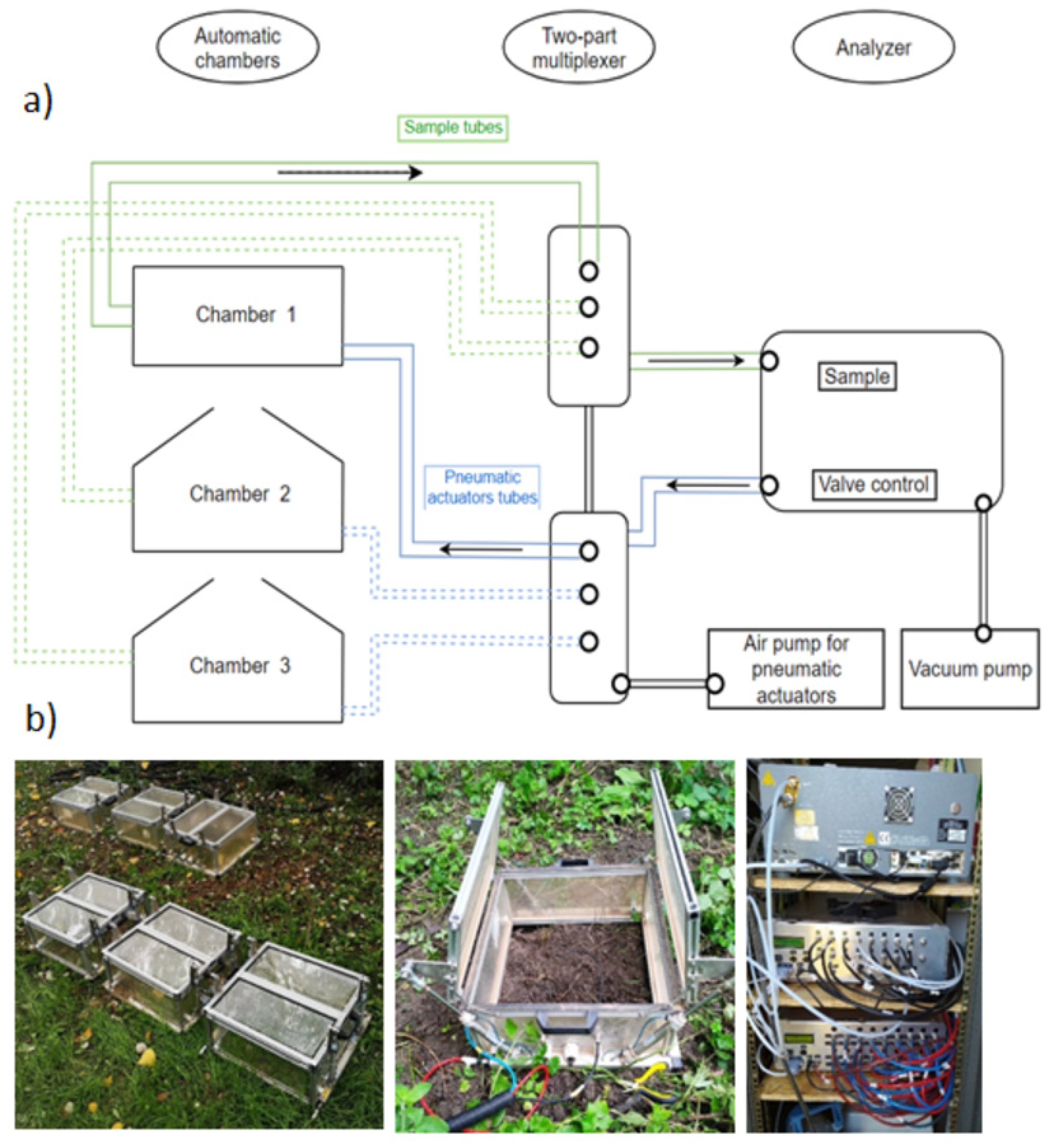
Figure 2.
Schematic representation of the dynamics in the chambers showing the main parameters that are used for the calculation of the fluxes.(1 column).
Figure 2.
Schematic representation of the dynamics in the chambers showing the main parameters that are used for the calculation of the fluxes.(1 column).
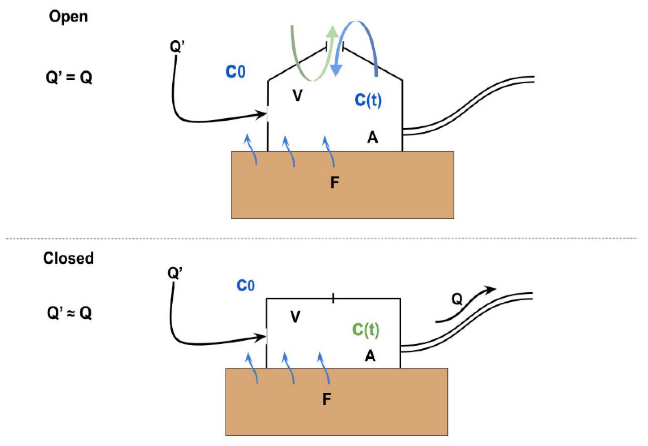
Figure 3.
The flux F to be estimated can be found as using a linear regression of concentration data c(t) against a transformed time variable g(t). Panel (a) shows the linear regression with transformed time and panel (b) shows the same result back-transformed to the time domain. (2 columns).
Figure 3.
The flux F to be estimated can be found as using a linear regression of concentration data c(t) against a transformed time variable g(t). Panel (a) shows the linear regression with transformed time and panel (b) shows the same result back-transformed to the time domain. (2 columns).
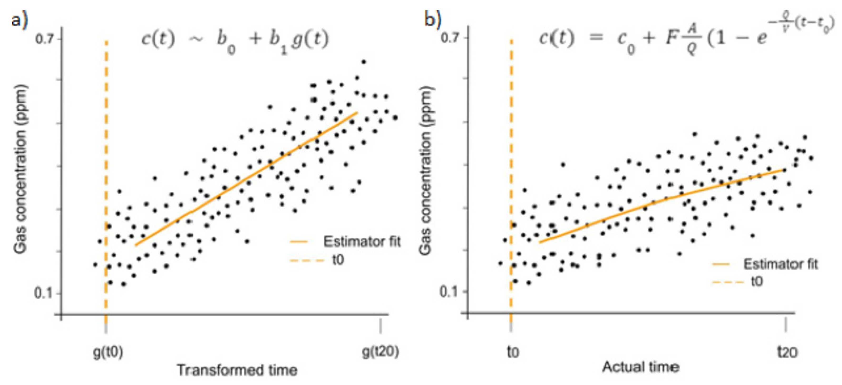
Figure 4.
Due to the delay caused by the length of the tubes, the data collected during one chamber’s closure corresponds to data from to the previous measure. The software discards this few initial minutes and makes the estimation of the flux with the remaining data. (1 column).
Figure 4.
Due to the delay caused by the length of the tubes, the data collected during one chamber’s closure corresponds to data from to the previous measure. The software discards this few initial minutes and makes the estimation of the flux with the remaining data. (1 column).
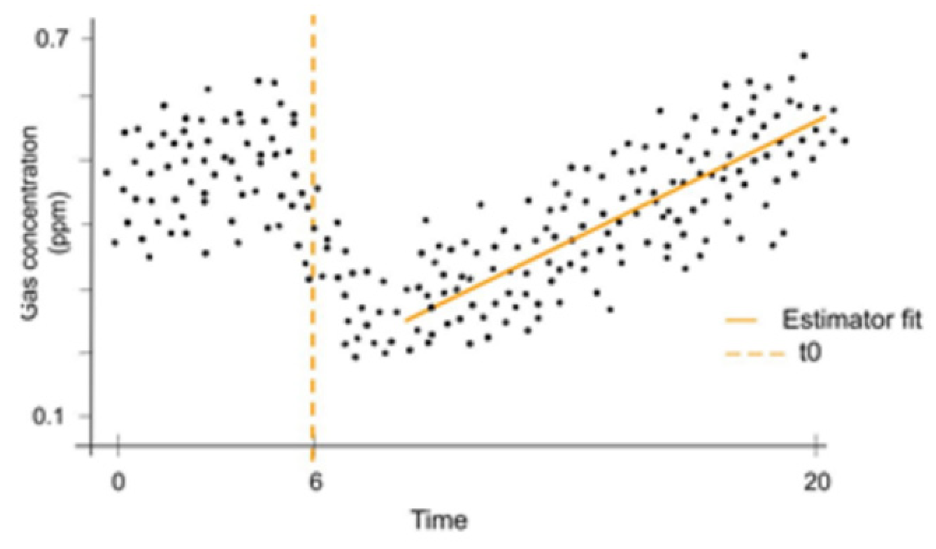
Figure 5.
Schematic figure of the steps to follow when using the software. First, the configuration file is adapted to the input data and physical equipment. Second, the import command incorporates the input data into an internal database. Third, fluxes are estimated using the fluxes command. Fourth, visualizations of each curve fit can be generated using the plot command. There is an additional command, info, giving summary information about the internal database for diagnostics. (2 columns).
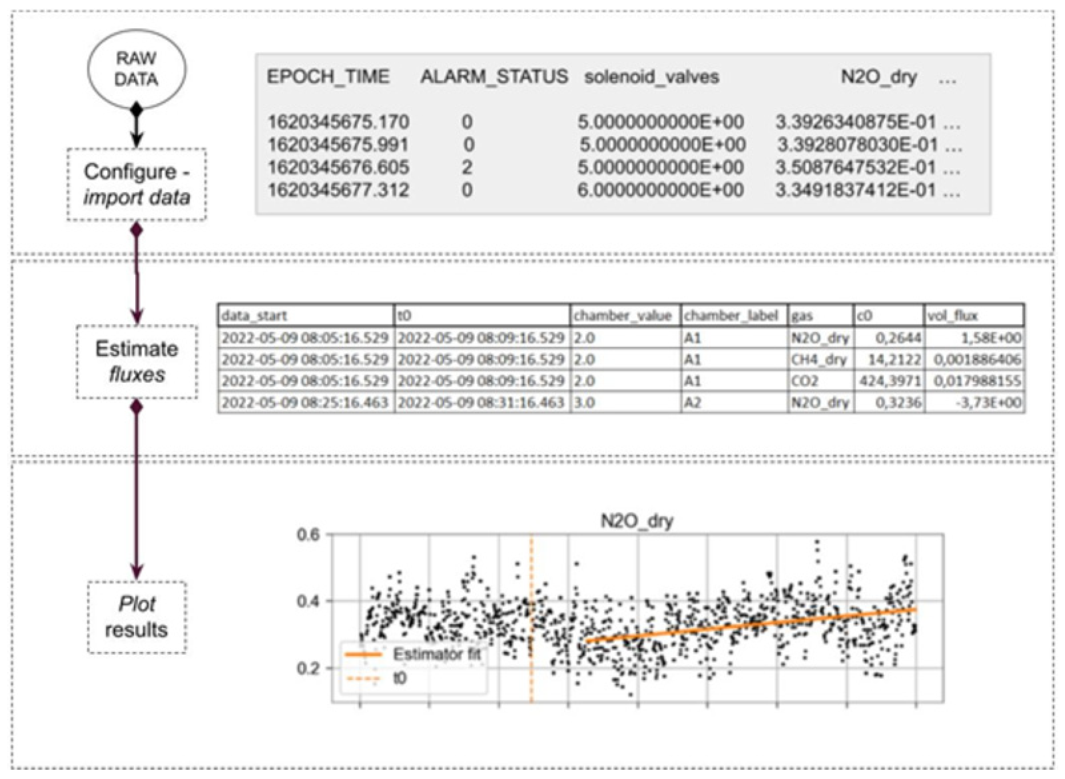
Figure 6.
Fragment from one file of raw data from the analyzer containing about 37 columns in total. Each of these files contain 1 hour of data, 24 files per day.(1 column).
Figure 6.
Fragment from one file of raw data from the analyzer containing about 37 columns in total. Each of these files contain 1 hour of data, 24 files per day.(1 column).
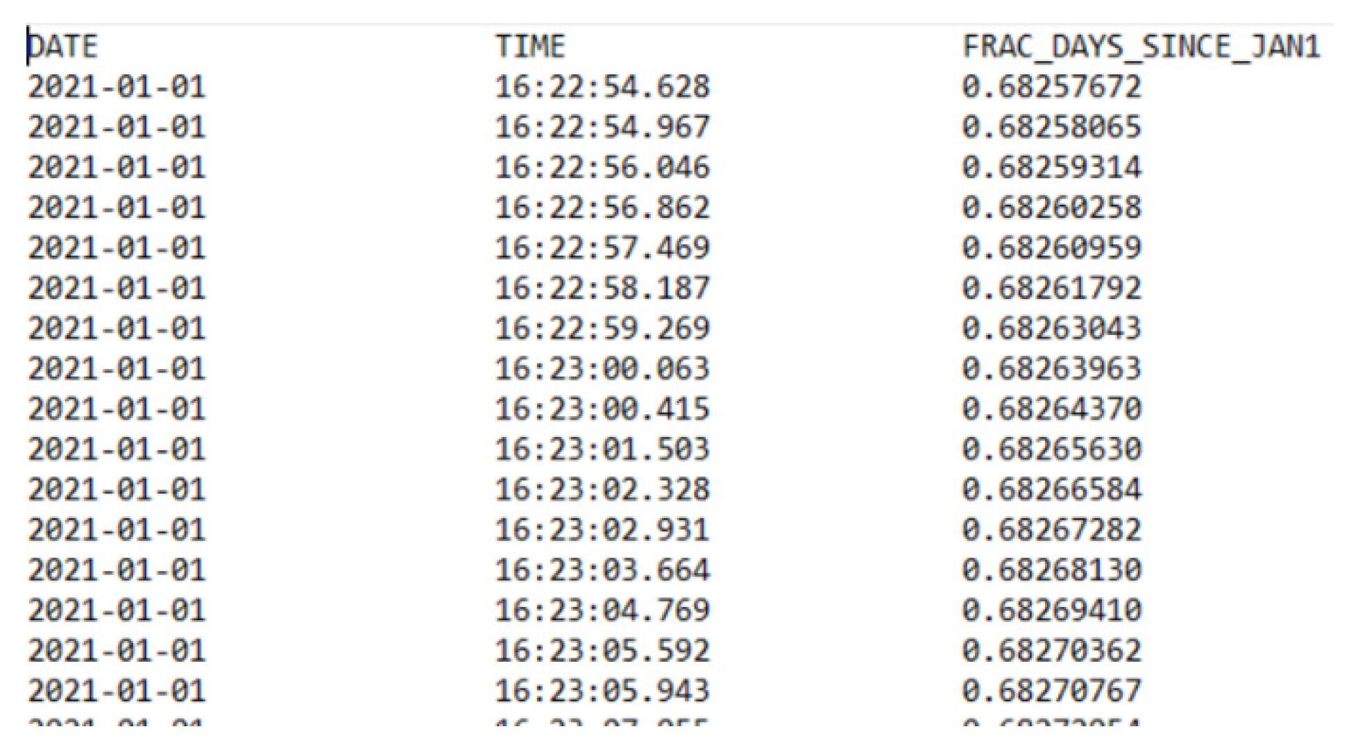
Figure 7.
Three consecutive measurements in chamber number 1, 2 and 3 with the estimation of the curve for each gas. At first look, those three measurements seem to present a normal dynamic, but the last image shows a different pattern indicating a potential error during the measurement. (2 columns).
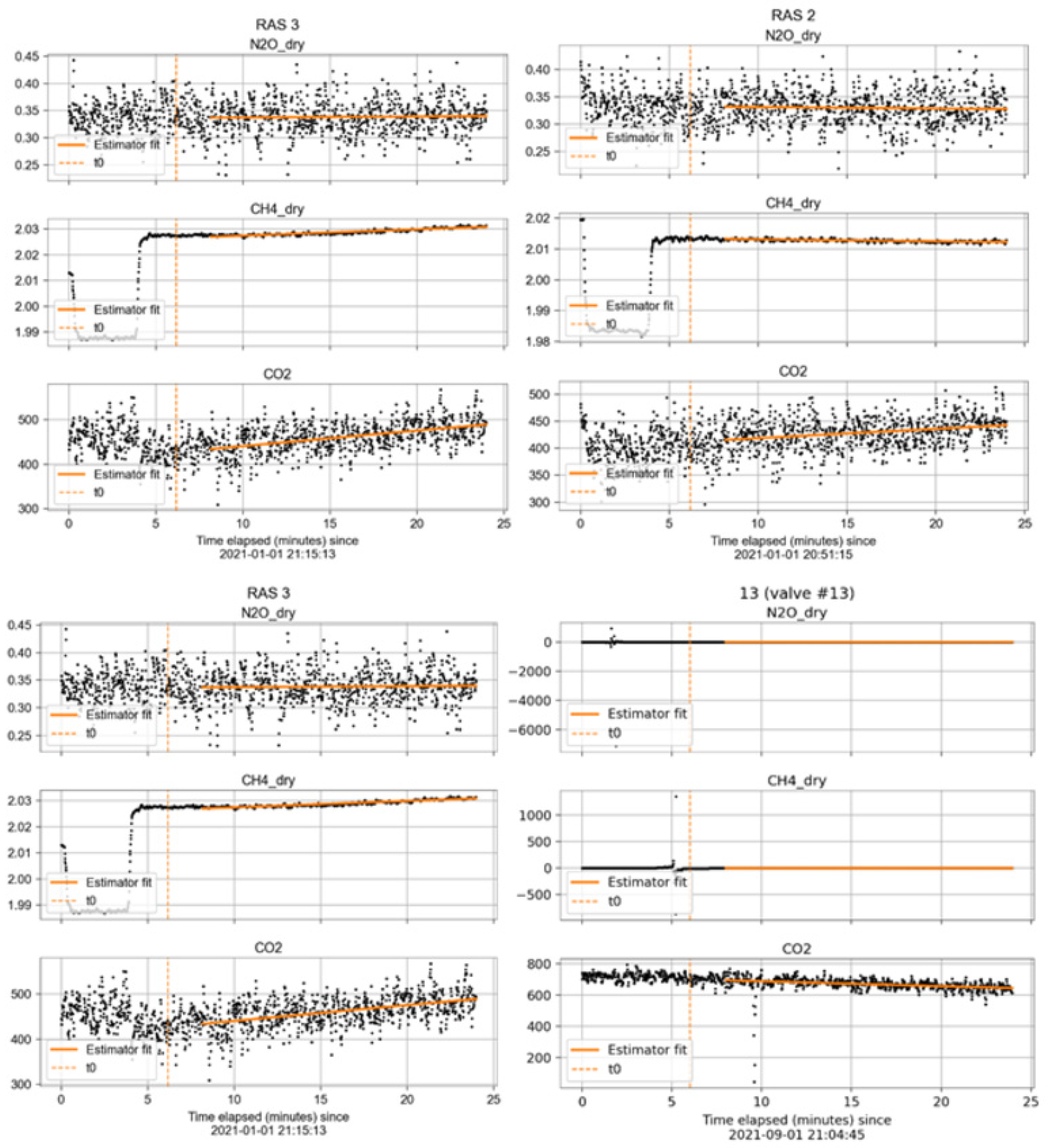
Figure 8.
Daily mean N2O emissions per chamber during January 2021. To easily distinguish the trends, only one repetition of each treatment is represented with the name “RAS” and its corresponding number. The emission along the month shows a significant growth at the end coinciding with a rewetting event. (1 column).
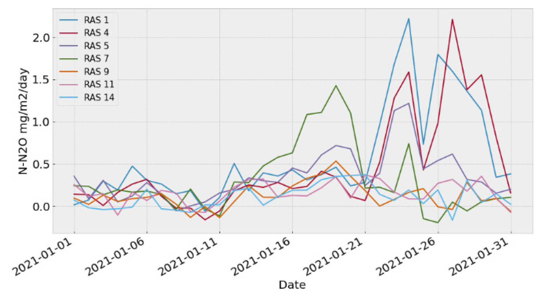

Table 1.
Imported data format and selected columns with the original column names in our raw data. We discard most of this data that is not useful for the calculations, and we keep 6 columns from the previous 37. These settings are configured in the .toml file. (1 column).
Table 1.
Imported data format and selected columns with the original column names in our raw data. We discard most of this data that is not useful for the calculations, and we keep 6 columns from the previous 37. These settings are configured in the .toml file. (1 column).
| Selected Data | Data Format |
| A timestamp of the sample: EPOCH_TIME | float64 |
| Current measuring chamber: SOLENOID_VALVE | float16 |
| Type of alarm if raised: ALARM_STATUS | int8 |
| CO2 Concentration: CO2 | float32 |
| N2O Concentration: N2O_dry | float32 |
| CH4 Concentration: CH4_dry | float32 |
Table 2.
Parameters, units, and values used in the calculations of the fluxes for this example. Chamber size, volume, and air flow of the gas from the chamber to the analyzer are required and may vary between equipment.(1 column).
Table 2.
Parameters, units, and values used in the calculations of the fluxes for this example. Chamber size, volume, and air flow of the gas from the chamber to the analyzer are required and may vary between equipment.(1 column).
| Parameter | Value And Units | Meaning |
| A | 0.25 m2 | Area occupied by the chamber on the soil. |
| Q | 4.17e-6 m3/s (0.25 liter/minute) |
Air flow through the tube carrying the sample. |
| V | 50e-3 m3 (50 liters) |
Volume of the chamber. |
Table 3.
Selected columns for our tabulated data. (1 column).
| column name | Description |
| data_start | The timestamp of the measurement’s first sample |
| chamber_value | Current measuring chamber |
| chamber_label | Name of the sampling point measuring |
| t0 | Initial time for the estimation fit |
| gas | Name of the gas measured |
| volumetric_flux | Value of the gas flux measured at the time |
Disclaimer/Publisher’s Note: The statements, opinions and data contained in all publications are solely those of the individual author(s) and contributor(s) and not of MDPI and/or the editor(s). MDPI and/or the editor(s) disclaim responsibility for any injury to people or property resulting from any ideas, methods, instructions or products referred to in the content. |
© 2023 by the authors. Licensee MDPI, Basel, Switzerland. This article is an open access article distributed under the terms and conditions of the Creative Commons Attribution (CC BY) license (http://creativecommons.org/licenses/by/4.0/).
Copyright: This open access article is published under a Creative Commons CC BY 4.0 license, which permit the free download, distribution, and reuse, provided that the author and preprint are cited in any reuse.


