Submitted:
11 October 2024
Posted:
14 October 2024
You are already at the latest version
Abstract
The extent of single- and multi-cropping systems in any region, and potential changes to it, have consequences on food and resource use, raising important policy questions. However, addressing these questions is limited by a lack of reliable data on multi-cropping practices at a high spatial resolution, especially in areas with high crop diversity. In this paper, we describe a relatively low-cost and scalable method to identify double-cropping at the field-scale using satellite (Landsat) imagery. The process combines machine learning methods with expert labeling. We demonstrate the process by measuring double-cropping extent in a portion of Washington State in the Pacific Northwest United States--- a region with significant production of more than 60 distinct types of crops including hay, fruits, vegetables, and grains in irrigated settings. Our results indicate that the current state-of-the-art methods for identifying cropping intensity---that apply simpler rule-based thresholds on vegetation indices---do not work well in regions with a high crop diversity, and likely significantly overestimate double-cropped extent. Multiple machine learning models were able to perform better by capturing nuances that the simple rule-based approaches are unable to. In particular, our (image-based) deep learning model was able to capture nuances in this crop-diverse environment and achieve a high accuracy (96-99% overall accuracy and 83– 93% producer accuracy for the double-cropped class with standard error of less than 2.5%) while also identifying double-cropping in the right crop types and locations based on expert knowledge. Our expert labeling process worked well and has potential as a relatively low-cost, scalable approach for remote sensing applications. The product developed here is valuable to inform several policy questions related to food production and resource use.
Keywords:
double cropping
; multi cropping
; cropping intensity
; Landsat
; NDVI
; remote sensing
; machine learning
1. Introduction
Spatially-explicit characterization of land cover and land use, and how it changes over time is key to long-term agricultural, environmental, and natural resources planning and management. One land use characteristic that is becoming increasingly relevant for a wide range of policy questions is the extent of single-cropping versus multi-cropping systems; the latter refers to multiple crops grown and harvested in the same field in the same year. For example, government subsidized insurance for farmers that multi-crop has been proposed as a way to increase production and keep food prices down [1]. Additionally, climate change has the potential to disrupt single-cropping systems in positive and negative ways. On the positive side, longer growing seasons under warming can allow cooler regions that historically could only single-crop to transition into multi-cropping systems [2] and increase total food production and make farming more profitable. On the negative side, such a switch can increase crop irrigation water demands exacerbating water security concerns [3]. It may also increase fertilizer use, exacerbating nutrient loading problems in water bodies, and negatively affecting soil health in general [4,5].
Over the last decade, several studies have utilized satellite imagery and mapped cropping intensities, where an intensity of 1, 2 and 3 are indicative of single-, double- and triple-cropping, respectively. While earlier work utilized coarse-spatial-resolution imagery at 0.5 to several kilometer resolution [6,7,8,9], recent work has focused on Landsat or Sentinel data at finer spatial resolutions of 10m to 30m [10,11,12,13]. With the exception of [13]—a global spatially-explicit product building on methodology from [10]—work has primarily focused on geographic regions with high current multi-cropping-extent such as part of China, India and Indonesia. Regions such as the irrigated Western United States (US) where the multi-cropping practice is less prevalent historically but has potential to increase under a changing climate, are largely ignored. Additionally, crop diversity in the irrigated Western US is very high (hundreds of crops) as compared to the handful crop types typically referenced in existing work. It is unclear if the methodology used in the existing work will translate well into areas of high crop diversity.
The typical methodologies used in quantifying cropping intensities are rule-based. They use a vegetation time series, apply threshold rules to identify peaks and troughs or starts and ends of the season, and count the number of crop cycles. Please note that by time series, we refer to the sequence of vegetation index over a given year. Given that these vegetation index thresholds can vary by crop and region, some modifications to generalize the process are considered. This includes standardization practices that replace the direct use of a vegetation-index time series with standardized values [10,13]. Additional enhancements to disregard spurious growth cycles are sometimes considered. For example, spectral indices indicative of bare soil such as the Land Surface Water Index (LSWI) are used to double check the start and ends of the season [9,11], especially when water-logged rice cropping systems are involved. A minimum crop-cycle-length constraint is also applied in some cases [10,13]. A key advantage of these methods is that a training dataset is not necessary.
While machine learning (ML) model applications—which require ground-truth datasets—are ubiquitous in applications like crop mapping, they are rare in crop intensity mapping [14,15] and absent in larger regional-scale applications of crop intensity mapping. However, these methods can be potentially helpful to learn important nuances in high-crop-diversity environments where vegetation thresholds and cycle lengths vary significantly by crop, soil characteristics, and farming practices (e.g. herbicide applications). Advantages of ML models are: (i) they will be more accurate as training set grows, (ii) they are more robust to rare or erroneous cases, and (iii) these methods learn mostly from frequent instances. The challenge in exploring ML methods is lack of ground-truth data (spatially-explicit labelled cropping intensity) across a range of cropping systems for training the models. While all labeling exercises are time and labor extensive, some applications such as the single-crop versus multi-crop distinction, are prohibitively so. For example, labeling images with irrigation canals or apples on a tree, can be performed by a human investigating the image once directly, and with relatively minimal training. In contrast, labeling fields as single- or multi-cropped requires hiring enough personnel to visit fields multiple times within a season, which quickly becomes time and cost prohibitive.
Our objective is to address the gap in field-scale single- and multi-cropped land use data availability in regions with high crop diversity. We address this by: (a) labeling a ground-truth dataset in a relatively low-cost and scalable manner, (b) developing and evaluating ML classification methods for single- and multi-cropped fields that are crop-agnostic and at a field-scale, and (c) comparing the performance of the ML models with a simpler rule-based method that is typically used. By low-cost we mean the relatively lower cost in terms of time and labor needs compared to drive-by/windshield surveys which are prohibitively expensive for our use case and not scalable to large areas. Finally, we will apply our best performing method to the irrigated agricultural extent of eastern Washington State in the Pacific Northwest US (Figure 1), as a case study. In this regional context, multi-cropping is essentially double-cropping and the rest of the paper uses this more specific terminology.
Our study region is a good test-bed for several reasons. Even though double-cropping is practiced, single-cropping dominates, posing a challenge for identifying double-cropped fields. It is located in the northern latitudes, and as the climate warms and the growing season lengthens, conditions could become more conducive for double-cropping. Additionally, it relies on surface water for irrigation, and there are important field-scale water management challenges associated with increased double-cropping, necessitating spatially-explicit information. This relates not just to the magnitude of additional irrigation water that might be needed, but also to the timing. Water law in the states in the Western US generally specifies that water rights are associated with a specific place and season of use and a new extended season of use brings in a regulatory burden on the water rights holder (farmer or irrigation district) and the managing agency (e.g. Washington State Department of Ecology) to modify the water right specifications accordingly. This is a time- and cost-intensive process as changes need to be verified under the stipulations of the Western Water Law and Prior Appropriation Doctrine [16,17].
While recent cropping-intensity studies have leveraged data from the Sentinel mission—providing a 10m spatial resolution with a 5-day revisit [18], we intentionally utilize data from the Landsat mission [19,20] at a 30m spatial resolution and an 8-day (when two concurrent Landsat products are combined) revisit. This allows future leveraging of the Landsat time-series going back several decades—invaluable to understand trends, drivers and impacts of adopting double-cropping.
For a low-cost labeling process that does not involve drive-by surveys multiple times within a season, we leverage satellite imagery and the knowledge of regional experts who are familiar with the cropping systems and fields. While this labeled dataset may not be as good as that from a drive-by survey, we expect that it will provide an adequate policy-relevant level of accuracy for identifying single- versus double-cropped extent. We develop and evaluate four ML models, and compare them with a traditional rule-based method that does not require ground-truthing to assess the importance of the labeling process. This is an important result for applying this method to other crop-diverse regions.
The products that come out of this research can inform many policy questions. Additionally, learnings from this case study can be applied more broadly to the development of land use datasets under the challenging contexts of prohibitively expensive costs in developing ground-truth datasets.
2. Methods and Data
The overall workflow components described in the this study are summarized in Figure 2. We first compute the field-scale smoothed NDVI time-series. This data along with other information is provided to the expert labeling process that creates the labeled ground-truth dataset. Classification models are then trained on the NDVI data and evaluated with the test set. Crop-specific summaries are also created for the test set. Finally, the models are applied over the full study area to obtain annual spatial-explicit maps of double-cropping.
Our unit of analysis is a field-level rather than pixel-level analysis, because that is the decision scale and because pixel-level analysis has challenges related to spatial correlations and within-field differences in classes across pixels [21]. Therefore this comes under the class of object-based analysis.
2.1. Input Datasets
The input data includes a time-series of a commonly used vegetation index—Normalized Difference Vegetation Index (NDVI) [22,23]— generated from multi-spectral observations at a 30m spatial resolution from 2015 to 2018 (Table 1) from Landsat 7 and 8. With two concurrent missions running at a staggered temporal resolution of 16 days, we get a combined finer temporal resolution of ∼8 days—important for capturing the quick succession of harvest and planting cycles in double-cropped systems. A field-scale NDVI time-series is obtained by averaging values across all pixels contained within a field. More details of the time-series construction are provided in Section 2.3. We would like to note that we did explore the Enhanced Vegetation Index (EVI) that address saturation issues with NDVI, but found no improved performance and do not report results with this index in the paper.
Field boundaries were obtained from the [24]. This dataset was created via drive-by surveys by WSDA covering approximately a third of the state each year. That is, sections of the study area (Figure 1) were surveyed at least once over a three-year period. Each year’s dataset has the field boundary, crop type, irrigation system, and the survey date. The crop type recorded is just the main crop that was observed at the time of the annual drive-by survey. That is, information on double-cropping is not present in this dataset as that would require multiple drive-by passes by the same field each year.
To create a ground-truth set, we only consider fields that were surveyed in the year under consideration so that the field boundaries and crop-types are accurate (see Section 2.2 for the labeling process). We used data from the years 2015 to 2018, which resulted in 44,850 fields. Fields smaller than 10 acres were removed from the analysis to avoid edge-effects, which result in a noisy vegetation index signal. These smaller fields comprise less than 8% of the total area that we consider, and are rarely double-cropped according to the experience of our experts. Therefore, their exclusion will have a minimal impact on our analysis. We also filtered out crop types with minimal irrigated acreage (less than 2874.57 acres—11.63 km2) in the study area. We selected 10% of the fields from each crop for labeling and added additional fields by crop as necessary to ensure that we have at least 50 fields per crop (if available) in the labeled ground-truth dataset. The fields were sampled from each crop individually with stratified sampling following best practices suggested by Stehman and Foody [21].
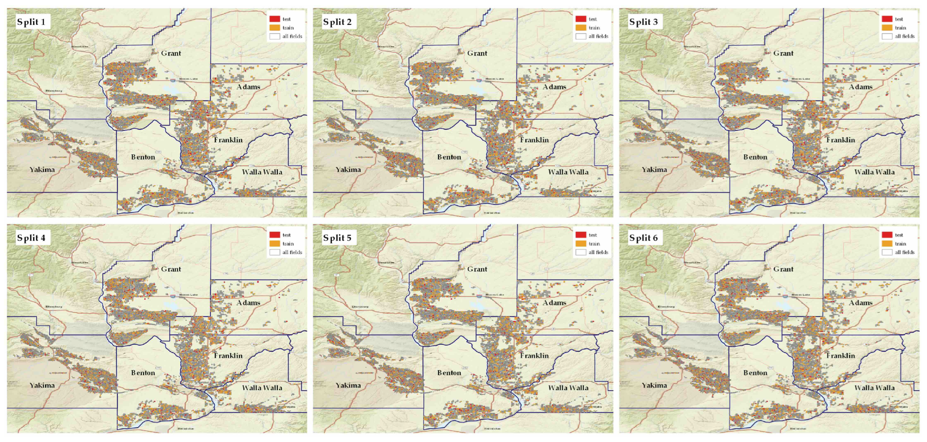
Figure 3 shows distribution of ground-truth set. The yellow dots are the fields used for training and the red dots are the fields in the test set. As we can see the fields are spread uniformly across the study region. For the final model application, we covered the entire irrigated extent in our counties of interest (Figure 1).
2.2. Expert Labeling Process
We collaborated with three individuals with extensive knowledge of cropping patterns in the region of study based on considerable time on the ground directly observing production. These individuals are professionals with university extension and governmental agricultural agencies. Such experts are present in many agriculturally intensive production regions, which adds to the repeatability of our approach to other areas.1 Using multiple labelers aligns with recommendation from [21] which states “protocols should be in place to monitor and evaluate the quality of the reference data and results. An example of quality assurance would be to evaluate consistency of reference class labels obtained by different interpreters.”
We had a three-step process for interacting with the expert panel. First, was a meeting that allowed for a more open ended discussion to identify crops and regions most associated with double-cropping, the timing of planting and harvesting of the first and second crop, and potential complications such as cover crops or hay crops that are harvested multiple times in the growing season. Such open ended meetings are valuable for narrowing the scope of the analysis, although it is important to not allow existing perceptions that may be partially incorrect to influence the analysis. In our case, we took a nuanced position to cover-crops. While cover-crops are generally not considered a double-crop, since production is not harvested, we made an exception for the yellow-mustard cover-crop and categorized it as a double-crop because our interest is in the water footprint. Other cover-crops are planted very late in the season requiring minimal or no irrigation. In contrast, yellow-mustard is planted early enough to require significant irrigation. A research question focused on total production of food and fiber, but not on resource use intensity, may result in a different categorization. It is also important to recognize that it may not be possible to differentiate a double-crop from a mustard cover-crop given expected similarities in their time-series signatures of vegetation indices.
To provide some additional context on the type of issues that may be discussed at this phase, the following are examples of topics raised. Certain crops (e.g., buckwheat, beans, peas, sweet corn, seed crops, sudangrass, triticale in some regions, and alfalfa) are more prevalent in double-cropping systems and therefore it would be good to know the crop type for the labeling process. Certain irrigation systems (e.g., flood) are not typically seen in double-cropped fields and the irrigation system would also be useful information for the labeling process. Additionally, double-cropping is prevalent in some areas and with some growers, and having a mapped location of the field will assist the expert in labeling by leveraging their local knowledge. In a double-cropping system, the second crop is typically planted by early August at the latest, and any indication of a second planting much after that is either a fall planted crop for the following year or a cover crop which should be considered a single-crop system for our purposes.
The second phase of the expert panel interaction was asynchronous labeling. For each field, we provided the vegetation index time-series, the crop-type, irrigation system, and a google map link to the field location in a Google Form. The form had five choices for labels: “single crop”, “double crop”, “mustard crop”, “either double or mustard crop”, and “unsure”. Before finalizing the ground-truth set to be sent to the expert panel, four other team members labeled easy to categorize crops—including crops that were clearly single-cropped from a clean vegetation index time-series, and perennial tree crops and berries which we know cannot be double-cropped—and checked for agreement across team members. The remaining observations, that constitute the more difficult cases, were labeled by experts asynchronously with each field labeled by at least two experts.
We flagged the fields where the experts were not in agreement and resolved discrepancies during a final synchronous meeting. Some challenging discrepancies could not be resolved and 15 fields were left as unsure and omitted from our dataset. The final labeled dataset consisted of 3,160 fields across four years (2015-2018) and representative of 63 crops Table 2 and five counties Table 1. The labeling process was guided by more information than just the vegetation index time-series, which is the only training input to the models.
2.3. Vegetation Index Time-Series
Crops have distinct spectral reflectance signatures related to their growth and phenological stages. In remote sensing applications, this is typically captured via vegetation indices that capture growth condition, phenology, and canopy cover of plants as the season progresses. While many vegetation indices exist, a commonly used one in agricultural contexts is the Normalized Difference Vegetation Index (NDVI) [10,12,25] which is calculated from spectrometric reflectances in the red and near-infrared bands (Equation (1)). NDVI steadily increases after planting and decreases with senescence leading to harvest. We used the Google Earth Engine (GEE)—a geospatial processing platform that helps access the large suite of publicly available satellite imagery—to obtain field-scale NDVI time-series. We used Landsat Level 2, Collection 2, Tier 1 products that contain atmospherically corrected surface reflectance bands2.
Satellite images are negatively affected by poor atmospheric conditions such as clouds or snow. These adverse effects typically lead to lower values of NDVI. As a part of data collection from GEE, we remove the we already said it just above: cloudy pixels and then compute the average field-scale NDVI using the remaining clean pixels. Taking the average across pixels is a standard and routine practice [28,29]. After fetching the data we remove noise from time-series to smooth the bumps and kinks that could throw off the detection of the crop growth cycle. There are numerous ways of smoothing including weighted moving averages, Fourier and wavelet techniques, asymmetric Gaussian function fitting, and the double logistic techniques. For comparison of different smoothing methods please see [30,31,32,33,34]. Performance of these methods depends on the data, the vegetation type, the data source, and the task at hand [31,32]. We use Savitzky-Golay (SG) [31,35] which is a commonly used polynomial regression fit based on a moving window. By varying the degree of polynomial and the size of window one can adjust level of smoothness.
Positive values of NDVI are indicative of greenness and negative values represent lack of vegetation where NDVI varies between -1 and 1.
The following steps are performed for denoising.
- Correct big jumps. The process of growing, and consequently the temporal pattern of greenness cannot have abrupt increases within a short period of time. Therefore, if the NDVI increases too quickly from time t to , a correction is required. In such cases, we assume NDVI at time t is affected negatively and therefore, we replace it via linear interpolation. In our study, we used a threshold of as the maximum NDVI growth allowed per day.
- Set negative NDVIs to zero. Negative NDVI values are an indication of lack of vegetation. In our scenario, the magnitude of such NDVIs are irrelevant. The negative NDVIs with high magnitudes adversely affect the NDVI-ratio method for classification and therefore the negative values are set to zero. Assume there is only one erroneous NDVI value that is negative and large in magnitude; e.g. -0.9, while all other values are positive. Then, the NDVI-ratio method which looks at normalized NDVI values will have a large value in its denominator and this single point affects the other points’ standardized values which can throw off the NDVI-ratio method. Under this scenario, the NDVI-ratio at the time of trough will be pushed up which leads to missing the harvest and re-planting in the middle of a growing year.
- Smooth the time-series. As the last step, the SG filter is applied to time-series to smooth them even further. SG filtering is a local method that fits the data with a polynomial using the least square method. The parameters used in this study are 3 for the degree of polynomial and 7 for the size of moving window; i.e. a polynomial of degree 3 is fitted to 7 data points.
2.4. Models
With the labeled data and vegetation index time-series, we develop and evaluate 5 models to classify fields as single- or double-cropped. This includes the NDVI-ratio method used in prior related works [10,13], and four ML models; random forest (RF), support vector machine (SVM), k-nearest neighbors (kNN), and deep learning (DL).
- Train and test datasets
- A stratified splitting across crops (see Section 2.1) is applied to the ground-truth set six times to get six sets of 80% of training and 20% of testing subsets. Within the 80% training data, a 5-fold cross-validation (train-validation split) was used to train the ML models.
- NDVI-ratio method.
-
One widely used approach for detecting the start of the season (SOS) and end of season (EOS) is the so-called NDVI-ratio method of [38]. NDVI-ratio is defined bywhere is NDVI at a given time, and are minimum and maximum of NDVI over a year, respectively. When this ratio crosses a given threshold, [10,13], then there is a SOS or EOS event. One pair of (SOS, EOS) event in a season is indicative of single cropping, and two pairs are indicative of double cropping. The following rules are applied under the NDVI-ratio method scenario.
- If the range of NDVI during the months of May through October (inclusively) is less than or equal to 0.3, then this field is labeled as single-cropped. This step was motivated by the low and flat time-series of vegetation indices exhibited by orchards during visual inspection of figures.
- Determine SOS and EOS by -ratio method.
- If an SOS is detected for which there is no EOS in a given year, we nullify such SOS. Such event occurs for winter wheat for example. Similarly, if we detect one EOS over the year with no corresponding SOS, we drop the EOS and consider it as a single-cropping cycle. Example is winter wheat that is planted in the previous year.
- A growing cycle cannot be less than 40 days.
- Machine learning models.
-
We build three statistical learning models—SVM, RF, and kNN—as well as a DL model for classification. Given that the kNN model computes the distance between two vectors (NDVI at multiple points in time), the vectors need to be comparable. Planting dates may vary by field, and therefore, the measurement for distance should take the time shift into account. This is accomplished by using dynamic time warping (DTW) as the distance measure for the kNN model. DTW was introduced by Itakura [39] in an speech recognition application and now is used in a variety of applications including agriculture [14,40]. It measures the distance between two time-series and takes into account the delay that may exist in one of the time-series; it warps time to match the two series so that the peaks and valleys are aligned.For deep learning we have used the pre-trained VGG16 model provided by Keras and trained only the last layer to avoid overfitting problem. While the SVM, RF, and kNN models are provided with a vector of NDVI values as input, the DL model is provided with NDVI time-series images as inputs. This means that our approach to DL falls under the category of image classification. While time-series data are not usually analyzed in this manner [41], it allows for nuances in the shape of the time-series that other models may not capture, potentially resulting in better performance.Given that there are fewer double-cropped than single-cropped fields, we oversampled the double-cropped instances (the minority class) to address the class imbalance in the dataset. After oversampling, number of instances in the minority class was less than 50% of number of instances in majority class. Oversampling more than 50% led to lower performance. The problem, of course, is not the “imbalanced-ness”. The problem is that each class invades the space of the other class [42,43] and overdoing oversampling contributed to lowering the performance in our case. Please note that there is no oversampling in the NDVI-ratio method, since there is no training involved and the rules in NDVI-ratio method are pre-defined. These rules are applied to each individual field independent of other fields. In ML, however, all data points play a role in determining the shape of the classifier. Thus, oversampling is an attempt to tilt the weight in favor of the minority class.The training process was optimized using 5 fold cross-validation. The models are implemented using the Python (v3.9.16), scikit-learn package (v1.2.1) for RF, SVM, and kNN. For DTW metric used in kNN, dtaidistance v2.3.9 is used. For deep learning we have used TensorFlow (v2.9.1) and Keras (v2.9.0)3.
- Accuracy assessment
-
There are three accuracy metrics used and presented in this study. Overall accuracy is used during training and for optimizing parameters and hyperparameters. For the testing phase, we report count-based overall, user’s and producer’s accuracies as well as their standard errors (SEs) following the methods described in [44] which accounts for the sampling strategy (e.g. stratifications).Unlike overall accuracy, user’s and producer’s accuracies provide information of errors associated with each specific class. Producer’s accuracy helps identify consistent under-representation of a class on a map while the user’s accuracy indicates if a class is consistently mislabeled as another class. The producer’s accuracy (for double-cropped class) refers to the fraction of true double-cropped fields that were predicted as double-cropped and the user’s accuracy refers to the fraction of predicted double-cropped fields that were actually double-cropped.
3. Results
In this section, we compare the performance of the ML models against each other and the NDVI- ratio method. We present crop-specific and regional summaries on the test dataset, and apply the DL model to all the fields in the study region for specific years (Table 1) reflective of “current” double-cropping extent.
3.1. Accuracy Statistics
In this section we present the result of classifying the test sets with the trained models. The four ML models, outperform the NDVI-ratio method with overall accuracies ranging from 95% to 99% as opposed to 89-91% (Table 3) across the 6 test sets. Individual model performance is provided in Table A1 in the Appendix A. Additionally, user’s accuracy of NDVI-ratio method is poor (46-54%) with significant over-prediction of single crops as double crops.
The DL has the best overall performance and the DL and SVM models have the best performance in identifying double-cropped fields (Table 3). The RF model has relatively higher user’s accuracy than producer’s accuracy unlike other models. The implication is that the RF model is less likely to mislabel single-crops as double-crops while the DL and SVM models are less likely to mislabel double-crops as single-crops.
The standard errors of overall accuracy are between 0.1 and 0.8% and are fairly consistent across all models (Table 4). For the double-cropped fields the range for standard errors of producer’s and user’s accuracies are 0 to 5.4% and 1.2% to 6.4%, respectively, across all models. The DL model has a narrow range of standard error (0 to 2.5%) for producer’s accuracy (for double-cropped fields).
Figure 4 shows NDVI time series for four fields labeled by the DL model. Two fields are labeled correctly (Figures 4a and 4b) and two are labeled incorrectly (Figures 4c and 4d). For the field shown in Figure 4c the model has missed the fact that the second crop’s cycle is a bit too late in the season (starting in September). In Figure 4d, where the model incorrectly labeled a double-cropped field as a single-crop, the noise in the raw data (red dots), seems to have resulted in an over-smoothing (blue line) misleading the model.
While the above statistics are field count-based, confusion matrix for proportion areas of single- and double-cropped extent are provided in Table A2 in Appendix A. The proportion area predicted as double-cropped by the DL models ranged from 11% to 14% while the ground-truth area proportion ranged from 13% to 17% across the test sets. Note that these statistics must be interpreted with caution as our study is object-based (see the Accuracy assessment in Section 2.4).
3.2. Fraction of Double-Cropped Acres by Crop
In our initial meetings with the experts, the following were identified as common double-cropped crops: buckwheat, beans, peas, sweet corn, seed crops, sudangrass, triticale (in some regions), and alfalfa. Based on our crop-wise classification statistics on the test dataset (Figure 5), the crops with relatively higher fractions match with this list, except for alfalfa. Alfalfa is a perennial crop with a 3- to 4-year cycle where double cropping is a possibility only in the final year of the cycle. Given this, our labeling in the training set skewed toward classifying it as a single crop, and we may be underestimating the double-cropped acres for this crop.
The high percentages of buckwheat and yellow mustard are in agreement with the local knowledge that buckwheat is almost always double-cropped, and that yellow mustard primarily is a cover-crop following a potato crop. This is in contrast with the mustard crop-type that is grown as a seed crop with a low double-cropped fraction. Moreover, perennial tree fruit and berries such as apples and blueberries cannot be double-cropped and the model performs well in capturing them as single-crops (only 2 out of 8,429 fields were incorrectly labeled). While all models are generally in agreement across crops, the differences across models are larger for some crops (e.g., triticale hay, mustard, and buckwheat).
3.3. Regional Summary and Spatial Distribution of Double-Cropped Fields
Over the 6 counties analyzed, around 10% of the total irrigated extent was double-cropped based on the best DL model. While we do not have the ground-truth data to compare this overall number, it is in qualitative agreement with the anecdotal expectation and local experts’ knowledge that the region has some but not a lot of double-cropped extent.
The majority of double-cropped fields are in the United States Bureau of Reclamation’s Columbia Basin Irrigation Project area that covers parts of Franklin, Adams, and Grant counties. The lowest rate of adoption is in Yakima county (Figures 6a and 6b). This is also in agreement with the experts’ expectations, and our knowledge of water rights security in the region [46,47]. Water use associated with growing two crops requires secure senior water rights, and the Columbia Basin Irrigation Project region has the water rights that can facilitate this. In contrast, a region like Yakima county has a large fraction of junior water rights holders for whom water rights restrictions may constrain the ability to adopt double-cropping.
4. Discussion
Two metrics indicate that our approach to identifying double- versus single-cropped fields works well and could be extended to other regions with crop diversity. The first is the high overall and producer accuracy of our DL model on the test sets. The second is the qualitative evidence that we are getting the overall double-cropped crop types, and spatial extent in line with experts’ expectations. Additionally, the DL model has less instances of mislabeling double-cropped as single-cropped, and therefore higher producer accuracies and lower standard errors for the double-cropped class. For some applications producer accuracies might be more important. For example, a policy maker interested in capturing the double-cropping extent for estimating the related water footprint, will likely prefer a higher producer accuracy.
While the adjusted NDVI-ratio method (with augmented auxiliary algorithms) performed well in identifying double and triple-cropped fields in other work [10], its performance was poor in our case with very low users accuracy (46-59%) and over-prediction of double-cropped class. Note this is not a direct comparison because (a) the geographic area is different, (b) [10] is a pixel level analysis, while ours is object-based at a field-scale, (c) we exclude cover crops and focus on harvested crops which is consistent with the definition of multi cropping from a food security perspective and the NDVI-ratio methods are unlikely to be able to make this distinction unless a season definition is included, and (d) our methods have a training process that allows the model to learn more nuances related to the shapes of the vegetation time series as compared to simpler rule-based method. Therefore, while the diversity of crops in our region cannot be attributed as the sole reason for the difference in performance, it likely contributed to it. Each crop has different canopy cover and vegetation index characteristics, likely rendering one threshold value to be inadequate in capturing this diversity.
A more direct comparison is possible with a recent global spatially-explicit cropping-intensity product at a 30m resolution [13]. We overlaid the global product with our study region and identified the overlapping area for comparison. Given significant missing data in the global product in one of our counties of interest (Yakima county), we excluded that county from the comparison. We aggregated the pixel-level cropping intensity from [13] to our field-level to get the dominant intensity class. The resulting multi-cropped extent (primarily double-cropped) was ≈1,015.76km2 compared to our best DL model’s estimate of ≈ 437.06km2. Therefore, while the [13] global product is expected to be a conservative estimate in general, we find that it may be significantly overestimating the cropping intensity in our irrigated study area, and perhaps all of Western US irrigated extent. We hypothesize that this could be due to several reasons. First, the [13] methodology is based on an NDVI-ratio process which, as we demonstrated, does not work well and overestimates double-cropping in our highly diverse cropping environment. Additionally, our comparison highlighted that the [13] product seems to have erroneously classified a significant acreage of perennial crops (e.g., tree-fruit, berries, alfalfa) as double-cropped instead of single-cropped. This highlights that there is an opportunity to integrate ML methods that can be trained to capture additional nuance and regional insights into the global products to enhance their utility, especially in regions such as ours that are not well covered and tested in the cropping-intensity mapping literature. We acknowledge that this is more involved than rule-based methods where their simplicity is a strength for broad regional applications, but the benefits of trained models can be substantial in complex contexts and merit further exploration of ML approaches in crop intensity mapping.
The expert labeling process we describe here is much less burdensome than extensive drive-by surveys for land use labeling. The challenge is in identifying the right set of local experts for the application under consideration. At least in the United States agricultural context, the Land Grant University County Extension system has an established network of local experts that are familiar with the area, the fields, the growers, and their practices and are an excellent source of knowledge that should be leveraged more in developing labeled datasets that can aid remote sensing applications. While the precision of a drive-by survey may not be achievable, useful information for informing policy can be developed as demonstrated in this work.
This method has a number of potential extensions and applications. The first is extending the geographic scope of this work. While the model we have developed is publicly shared and can be directly applied, some additional labeling and retraining would likely be necessary, especially for regions where the cropping intensity can be larger than two crops in a year. Even in this scenario, our DL model can be used for transfer-learning approaches, which can shorten the training time. The models can be continually retrained and refined as new labeled data are created. While our ground-truth data collection and model development efforts focused on irrigated areas, the method is generic and should work for dryland regions as well, though this will need to be tested. Additionally, while our model development and application was at a field-scale, which is the scale of decisions, the method can be directly applied at a pixel scale as well in areas where field boundary data is not easily available.
The second is to apply the proposed method and develop a historical time-series of double-cropped extent. This would allow a trend analysis that could be used to identify drivers of increased or decreased double-cropping including changing climatic patterns and agricultural commodity market conditions [48]. Further analysis would be needed to isolate the climatic drivers of trends, but the methods and dataset developed here are an important first step in generating data that will facilitate these analyses. Climatic relationships, once established, can be be extrapolated in a climate-change context to quantify the potential for increased double-cropping in the future. When coupled with a cross-sectional analysis of historical double-cropping trends across diverse regions, climatic thresholds at which double-cropping becomes infeasible (e.g., because the summers are too hot to double-crop) can also be identified. This will provide a realistic upper bound of the potential for increased double-cropping.
Finally, from a water footprint perspective, this spatially-explicit dataset can be a valuable input to crop models (e.g., VIC-CropSyst [49]) to quantify irrigation demands under current and future conditions of double-cropping adoption. Existing studies on climate change impacts on irrigation demands do not account for double-cropping, and this addition will address an important missing component in the climate-change-impacts literature. This can inform the planning efforts of various stakeholders; irrigation districts planning for infrastructure management based on the season length, water rights management agencies planning for change requests, water management agencies planning for minimizing scarcity issues or changes to reservoir operations.
There are several other policy questions and trade offs that can be informed by utilizing such spatially-explicit datasets (along with other data and models). For example, how much of the growing global food demands can multi-cropping meet? Are the environmental outcomes of increased food production though intensification on existing land better or worse than outcomes from expanding agricultural land? What are the impacts on fertilizer inputs on the land or carbon sequestration potential? As stewards of our natural resources, it is important for us to address the broad range of trade offs that accompany any land use change trends and equip ourselves with datasets that help answer them.
5. Conclusion
The rule-based methods that are widely used to map cropping intensity did not work for our high-crop-diversity context. In contrast, ML models, especially the DL model, were able to learn crop-specific nuances and achieved an overall accuracy of 96% to 99%, user’s and producer’s accuracy of 74 – 92% and 83 – 93% respectively for the double-cropped class, while also identifying double-cropping in the right crop types and locations based on expert knowledge. Given that these models require labeled ground-truth data, low-cost labeling efforts that leverage satellite imagery and experts’ knowledge will be key to expanding the availability of such land use data sets at global scales.
Given that these labeling efforts are likely to be local/regional endeavours, a centralized mechanism to publicly share these labeled datasets will allow the research community to make continued advancements in modeling the environment via remote sensing approaches. Availability of these datasets would be critical to answer key making policy-relevant questions related to food security and natural resources sustainability.
Author Contributions
writing, H.N., K.R., S.S., A.N.K, and M.B.; review and editing, H.N., K.R., S.S., M.B., M.L., P.B., T.W., and A.M.; project administration, K.R. and M.B.; formal analysis, H.N., K.R., S.S., A.N.K, and M.B.; investigation, H.N., K.R., M.L., S.S., and M.B. methodology, H.N., K.R., M.B., P.B., A.M, A.N.K, and T.W.; data curation, H.N.; visualization, H.N., S.S.; funding acquisition, M.B. and K.R.;
Funding
This research was funded by the National Aeronautics and Space Administration’s Western Water Applications Office (NASA WWAO) under Award Number 1667355 and the U.S. Geological Survey Award No. G16AP00090-0006 administered by the Washington State Water Research Center.
Data Availability Statement
The datasets generated during and/or analyzed during the current study are available from the corresponding author on reasonable request.
Acknowledgments
We thank the Washington State Department of Ecology, the Washington State Department of Agriculture, and the Oregon Water Resources Department for supporting this research. We thank Siddharth Chaudhary, Bhupinderjeet Singh, Sienna Alicea, and Daniel Chadez for assistance with field surveys. Furthermore, this research used resources of the Center for Institutional Research Computing at Washington State University.
Conflicts of Interest
The authors declare no conflict of interest. The funders had no role in the design of the study; in the collection, analyses, or interpretation of data; in the writing of the manuscript, or in the decision to publish the results.
Abbreviations
The following abbreviations are used in this manuscript:
| DL | Deep Learning, |
| DTW | Dynamic Time Warping, |
| EOS | End of Season, |
| GEE | Google Earth Engine, |
| GT | Ground-Truth, |
| kNN | k-Nearest Neighbors, |
| ML | Machine Learning, |
| NDVI | Normalized Difference Vegetation Index, |
| NDVI-R | NDVI-ratio, |
| OA | Overall Accuracy, |
| PA | Producer’s Accuracy, |
| RF | Random Forest, |
| SE | Standard Error, |
| SG | Savitzky-Golay, |
| SOS | Start of Season, |
| SVM | Support Vector Machine |
| UA | User’s Accuracy, |
Appendix A. Extras
Appendix A.1. Details on ML Methods
The cost function that is minimized in the ML models is overall accuracy. The parameters tried for each specific models to obtain best model is listed below.
- SVM
-
In SVM technique we applied a grid search over the following set of parametersRegularization parameter c ∈ {5, 10, 13, 14, 15, 16, 17, 20, 40, 80},class_weight∈ {balanced, uniform}.
- DL
- Since our ground-truth set is small and the shapes of the time-series are not complicated, we used a pre-trained VGG16 network (transfer learning) from keras package and only trained the last two layers (one fully connected layer with 128 neurons followed by a binary output layer). Training only two layers is one of the steps that decreases the possibility of overfitting. The activation functions used for these layers are relu and sigmoid, respectively.
- kNN
-
Parameters used for optimizing kNN are number of neighbors and the weight parameters;n_neighbors∈ {2, 4, 6, 7, 8, 9, 10, 11, 12, 13, 14, 15, 16, 17, 18, 19, 20},weights∈{uniform, distance}
- RF
-
For the random forest, the parameters we searched over arecriterionmax_depth∈ {2, 4, 6, 8, 9, 10, 11, 12, 13, 14, 15, 16, 18, 20 }min_samples_split∈ {2, 3, 4, 5 }max_features∈ {sqrt, log2, None},class_weight∈ {balanced, balanced_subsample, None}ccp_alpha∈ {0, 1, 2, 3},max_samples∈ {None, 1, 2, 3, 4, 5}
Appendix A.2. All Splits of Ground-Truth Set
We divided the ground-truth set into 80-20% sets of training and testing 6 different times in total. This helped us to check if the test set in the main body of the manuscript was accidentally an easy set to classify or perhaps the training set was rich enough to capture all the different patterns.
We report the different split results below. We emphasis that the results below are the output of applying the trained model to the test sets. In other words, test set is not used in the training process, and thus, any good result is not an indication of overfitting.

Table A1.
Classification results from the test sets. User and producer accuracies reported in this table are for double-cropped class. These statistics are count-based.
Table A1.
Classification results from the test sets. User and producer accuracies reported in this table are for double-cropped class. These statistics are count-based.
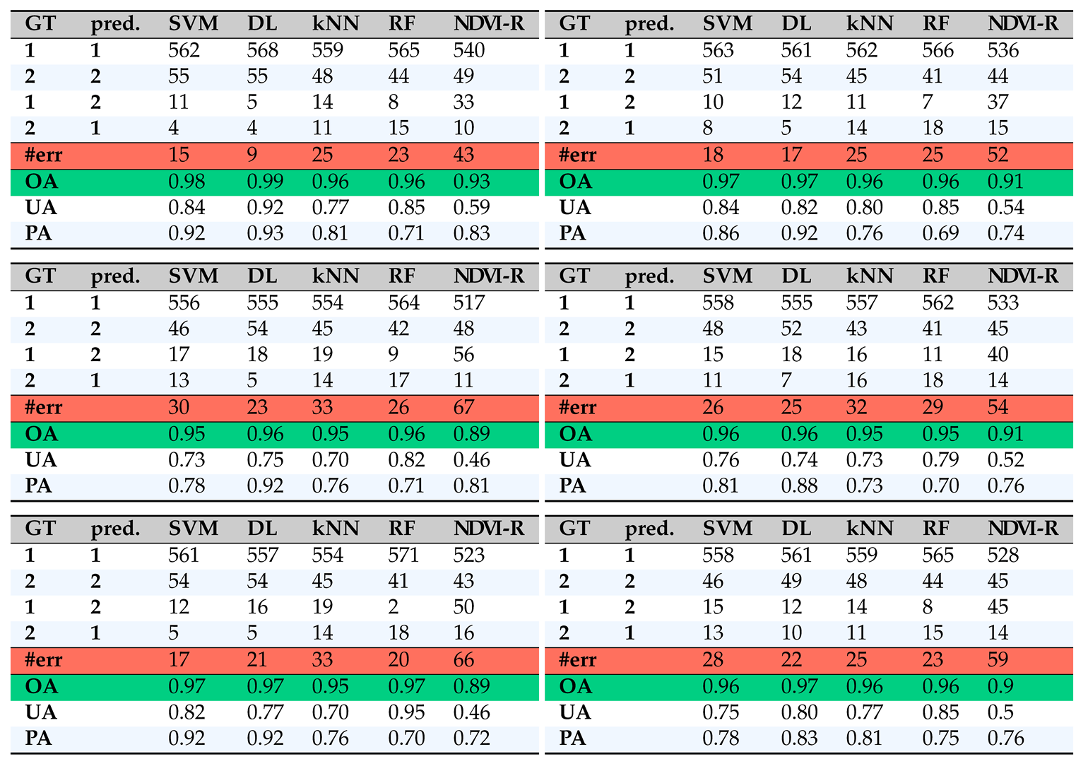
Table A2 presents the area-based confusion matrix. We, however, refrain presenting the accuracies based on the area since “in terms of the proportion of the area of the map that is incorrectly classified, an error for a large polygon has obviously more impact than an error for a smaller one” [50] .
Table A2.
confusion matrices based on field-area ratios for all 6 different splits of ground-truth dataset.
Table A2.
confusion matrices based on field-area ratios for all 6 different splits of ground-truth dataset.
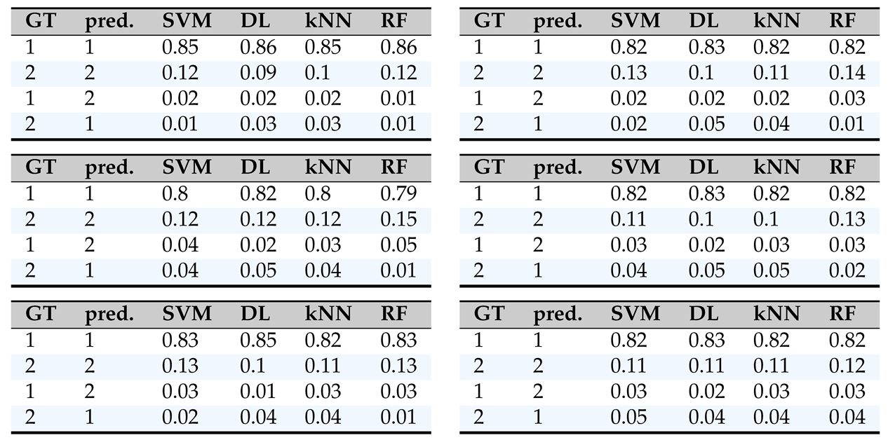
Figure A1.
All of the six splits of ground-truth set into training and test sets.
References
- Whitehouse Briefing. FACT SHEET: President Biden Announces New Actions to Address Putin’s Price Hike, Make Food More Affordable, and Lower Costs for Farmers. 2022. Available online: https://www.whitehouse.gov/briefing-room/statements-releases/2022/05/11/fact-sheet-president-biden-announces-new-actions-to-address-putins-price-hike-make-food-more-affordable-and-lower-costs-for-farmers/ (accessed on 28 October 2024).
- Seifert, C.A.; Lobell, D.B. Response of double cropping suitability to climate change in the United States. Environmental Research Letters 2015, 10, 024002. [Google Scholar] [CrossRef]
- Meza, F.J.; Silva, D.; Vigil, H. Climate change impacts on irrigated maize in Mediterranean climates: evaluation of double cropping as an emerging adaptation alternative. Agricultural systems 2008, 98, 21–30. [Google Scholar] [CrossRef]
- Lal, R. Soil carbon dynamics in cropland and rangeland. Environmental pollution 2002, 116, 353–362. [Google Scholar] [CrossRef] [PubMed]
- Jankowski, K.; Neill, C.; Davidson, E.A.; Macedo, M.N.; Costa Jr, C.; Galford, G.L.; Maracahipes Santos, L.; Lefebvre, P.; Nunes, D.; Cerri, C.E.; others. Deep soils modify environmental consequences of increased nitrogen fertilizer use in intensifying Amazon agriculture. Scientific reports 2018, 8, 13478. [Google Scholar] [CrossRef]
- Yan, H.; Xiao, X.; Huang, H.; Liu, J.; Chen, J.; Bai, X. Multiple cropping intensity in China derived from agro-meteorological observations and MODIS data. Chinese Geographical Science 2014, 24, 205–219. [Google Scholar] [CrossRef]
- Li, L.; Friedl, M.A.; Xin, Q.; Gray, J.; Pan, Y.; Frolking, S. Mapping crop cycles in China using MODIS-EVI time series. Remote Sensing 2014, 6, 2473–2493. [Google Scholar] [CrossRef]
- Ding, M.; Li, L.; Zhang, Y.; Sun, X.; Liu, L.; Gao, J.; Wang, Z.; Li, Y. Start of vegetation growing season on the Tibetan Plateau inferred from multiple methods based on GIMMS and SPOT NDVI data. Journal of Geographical Sciences 2015, 25, 131–148. [Google Scholar] [CrossRef]
- Biradar, C.M.; Xiao, X. Quantifying the area and spatial distribution of double- and triple-cropping croplands in India with multi-temporal MODIS imagery in 2005. International Journal of Remote Sensing 2011, 32, 367–386. [Google Scholar] [CrossRef]
- Liu, C.; Zhang, Q.; Tao, S.; Qi, J.; Ding, M.; Guan, Q.; Wu, B.; Zhang, M.; Nabil, M.; Tian, F.; others. A new framework to map fine resolution cropping intensity across the globe: Algorithm, validation, and implication. Remote Sensing of Environment 2020, 251, 112095. [Google Scholar] [CrossRef]
- Liu, L.; Xiao, X.; Qin, Y.; Wang, J.; Xu, X.; Hu, Y.; Qiao, Z. Mapping cropping intensity in China using time series Landsat and Sentinel-2 images and Google Earth Engine. Remote Sensing of Environment 2020, 239, 111624. [Google Scholar] [CrossRef]
- Pan, L.; Xia, H.; Yang, J.; Niu, W.; Wang, R.; Song, H.; Guo, Y.; Qin, Y. Mapping cropping intensity in Huaihe basin using phenology algorithm, all Sentinel-2 and Landsat images in Google Earth Engine. International Journal of Applied Earth Observation and Geoinformation 2021, 102, 102376. [Google Scholar] [CrossRef]
- Zhang, M.; Wu, B.; Zeng, H.; He, G.; Liu, C.; Tao, S.; Zhang, Q.; Nabil, M.; Tian, F.; Bofana, J.; others. GCI30: a global dataset of 30 m cropping intensity using multisource remote sensing imagery. Earth System Science Data 2021, 13, 4799–4817. [Google Scholar] [CrossRef]
- Rafif, R.; Kusuma, S.S.; Saringatin, S.; Nanda, G.I.; Wicaksono, P.; Arjasakusuma, S. Crop intensity mapping using dynamic time warping and machine learning from multi-temporal PlanetScope data. Land 2021, 10, 1384. [Google Scholar] [CrossRef]
- He, Y.; Dong, J.; Liao, X.; Sun, L.; Wang, Z.; You, N.; Li, Z.; Fu, P. Examining rice distribution and cropping intensity in a mixed single- and double-cropping region in South China using all available Sentinel 1/2 images. International Journal of Applied Earth Observation and Geoinformation 2021, 101, 102351. [Google Scholar] [CrossRef]
- Hutchins, W.A. Water rights laws in the nineteen western states; Number 1, Natural Resource Economics Division, Economic Research Service, US Department of Agriculture, 1971.
- Wiel, S.C. Water Rights in the Western States: The Law of Prior Appropriation of Water as Applied Alone in Some Jurisdictions, and As, in Others, Confined to the Public Domain, with the Common Law of Riparian Rights for Waters Upon Private Lands. Federal, California and Oregon Statutes in Full, with Digest of Statutes of Alaska, Arizona, Colorado, Hawaii, Idaho, Kansas, Montana, Nebraska, Nevada, New Mexico, North Dakota, Oklahoma, Oregon, Philippine Islands, South Dakota, Texas, Utah, Washington and Wyoming; Vol. 2, Bancroft-Whitney, 1911.
- Drusch, M.; Del Bello, U.; Carlier, S.; Colin, O.; Fernandez, V.; Gascon, F.; Hoersch, B.; Isola, C.; Laberinti, P.; Martimort, P.; others. Sentinel-2: ESA’s optical high-resolution mission for GMES operational services. Remote sensing of Environment 2012, 120, 25–36. [Google Scholar] [CrossRef]
- Lauer, D.T.; Morain, S.A.; Salomonson, V.V. The Landsat program: Its origins, evolution, and impacts. Photogrammetric Engineering and Remote Sensing 1997, 63, 831–838. [Google Scholar]
- Wulder, M.A.; Loveland, T.R.; Roy, D.P.; Crawford, C.J.; Masek, J.G.; Woodcock, C.E.; Allen, R.G.; Anderson, M.C.; Belward, A.S.; Cohen, W.B.; others. Current status of Landsat program, science, and applications. Remote sensing of environment 2019, 225, 127–147. [Google Scholar] [CrossRef]
- Stehman, S.V.; Foody, G.M. Key issues in rigorous accuracy assessment of land cover products. Remote Sensing of Environment 2019, 231, 111199. [Google Scholar] [CrossRef]
- Huang, S.; Tang, L.; Hupy, J.P.; Wang, Y.; Shao, G. A commentary review on the use of normalized difference vegetation index (NDVI) in the era of popular remote sensing. Journal of Forestry Research 2021, 32, 1–6. [Google Scholar] [CrossRef]
- Kriegler, F. Preprocessing transformations and their effects on multspectral recognition. Proceedings of the Sixth International Symposium on Remote Sesning of Environment, 1969, pp. 97–131.
- Washington State Department of Agriculture’s (WSDA) Agricultural Land Use Geodatabase. Accessed: 2024/10/28 12:33:10.
- Ghosh, A.; Nanda, M.K.; Sarkar, D. Assessing the spatial variation of cropping intensity using multi-temporal Sentinel-2 data by rule-based classification. Environment, Development and Sustainability 2022, 24, 10829–10851. [Google Scholar] [CrossRef]
- USGS Landsat 7 Level 2, Collection 2, Tier 1. Available online: https://developers.google.com/earth-engine/datasets/catalog/LANDSAT_LE07_C02_T1_L2/ (accessed on 28 October 2024).
- USGS Landsat 8 Level 2, Collection 2, Tier 1. Available online: https://developers.google.com/earth-engine/datasets/catalog/LANDSAT_LC08_C02_T1_L2/ (accessed on 28 October 2024).
- Belgiu, M.; Csillik, O. Sentinel-2 cropland mapping using pixel-based and object-based time-weighted dynamic time warping analysis. Remote Sensing of Environment 2018, 204, 509–523. [Google Scholar] [CrossRef]
- Huete, A.; Didan, K.; Miura, T.; Rodriguez, E.; Gao, X.; Ferreira, L. Overview of the radiometric and biophysical performance of the MODIS vegetation indices. Remote Sensing of Environment 2002, 83, 195–213. [Google Scholar] [CrossRef]
- Atkinson, P.M.; Jeganathan, C.; Dash, J.; Atzberger, C. Inter-comparison of four models for smoothing satellite sensor time-series data to estimate vegetation phenology. Remote Sensing of Environment 2012, 123, 400–417. [Google Scholar] [CrossRef]
- Cai, Z.; Jönsson, P.; Jin, H.; Eklundh, L. Performance of smoothing methods for reconstructing NDVI time-series and estimating vegetation phenology from MODIS data. Remote Sensing 2017, 9, 1271. [Google Scholar] [CrossRef]
- Geng, L.; Ma, M.; Wang, X.; Yu, W.; Jia, S.; Wang, H. Comparison of Eight Techniques for Reconstructing Multi-Satellite Sensor Time-Series NDVI Data Sets in the Heihe River Basin, China. Remote Sensing 2014, 6, 2024–2049. [Google Scholar] [CrossRef]
- Kandasamy, S.; Baret, F.; Verger, A.; Neveux, P.; Weiss, M. A comparison of methods for smoothing and gap filling time series of remote sensing observations-application to MODIS LAI products. Biogeosciences 2013, 10, 4055–4071. [Google Scholar] [CrossRef]
- Hird, J.N.; McDermid, G.J. Noise reduction of NDVI time series: An empirical comparison of selected techniques. Remote Sensing of Environment 2009, 113, 248–258. [Google Scholar] [CrossRef]
- Savitzky, A.; Golay, M.J. Smoothing and differentiation of data by simplified least squares procedures. Analytical chemistry 1964, 36, 1627–1639. [Google Scholar] [CrossRef]
- Kobayashi, H.; Dye, D.G. Atmospheric conditions for monitoring the long-term vegetation dynamics in the Amazon using normalized difference vegetation index. Remote Sensing of Environment 2005, 97, 519–525. [Google Scholar] [CrossRef]
- Liu, H.Q.; Huete, A. A feedback based modification of the NDVI to minimize canopy background and atmospheric noise. IEEE Transactions on Geoscience and Remote Sensing 1995, 33, 457–465. [Google Scholar] [CrossRef]
- White, M.A.; Thornton, P.E.; Running, S.W. A continental phenology model for monitoring vegetation responses to interannual climatic variability. Global Biogeochemical Cycles 1997, 11, 217–234. [Google Scholar] [CrossRef]
- Itakura, F. Minimum prediction residual principle applied to speech recognition. IEEE Transactions on Acoustics, Speech, and Signal Processing 1975, 23, 67–72. [Google Scholar] [CrossRef]
- Jeong, Y.S.; Jeong, M.K.; Omitaomu, O.A. Weighted dynamic time warping for time series classification. Pattern recognition 2011, 44, 9. [Google Scholar] [CrossRef]
- Ismail Fawaz, H.; Lucas, B.; Forestier, G.; Pelletier, C.; Schmidt, D.F.; Weber, J.; Webb, G.I.; Idoumghar, L.; Muller, P.A.; Petitjean, F. Inceptiontime: Finding AlexNet for time series classification. Data Mining and Knowledge Discovery 2020, 34, 1936–1962. [Google Scholar] [CrossRef]
- Prati, R.C.; Batista, G.E.; Monard, M.C. Data mining with imbalanced class distributions: concepts and methods. IICAI, 2009, pp. 359–376.
- Azhar, N.A.; Pozi, M.S.M.; Din, A.M.; Jatowt, A. An Investigation of SMOTE Based Methods for Imbalanced Datasets With Data Complexity Analysis. IEEE Transactions on Knowledge and Data Engineering 2023, 35, 6651–6672. [Google Scholar] [CrossRef]
- Stehman, S.V. Estimating area and map accuracy for stratified random sampling when the strata are different from the map classes. International Journal of Remote Sensing 2014, 35, 4923–4939. [Google Scholar] [CrossRef]
- Ye, S.; Pontius, R.G.; Rakshit, R. A review of accuracy assessment for object-based image analysis: From per-pixel to per-polygon approaches. ISPRS Journal of Photogrammetry and Remote Sensing 2018, 141, 137–147. [Google Scholar] [CrossRef]
- Weber, E.; Lee, B. Columbia basin project water authorizations. The Water Report 2021. [Google Scholar]
- Washington State Department of Ecology. Washington State Water Rights. Available online: https://appswr.ecology.wa.gov/waterrighttrackingsystem/WaterRights/Map/WaterResourcesExplorer.aspx (accessed on 28 October 2024).
- Borchers, A.; Truex-Powell, E.; Wallander, S.; Nickerson, C. Multi-cropping practices: recent trends in double-cropping 2014.
- Malek, K.; Stöckle, C.; Chinnayakanahalli, K.; Nelson, R.; Liu, M.; Rajagopalan, K.; Barik, M.; Adam, J.C. VIC–CropSyst-v2: A regional-scale modeling platform to simulate the nexus of climate, hydrology, cropping systems, and human decisions. Geoscientific Model Development 2017, 10, 3059–3084. [Google Scholar] [CrossRef]
- Radoux, J.; Bogaert, P. Good Practices for Object-Based Accuracy Assessment. Remote Sensing 2017, 9. [Google Scholar] [CrossRef]
| 1 | McGuire and Waters are county Extension professionals from our region of interest and Beale initiated and currently manages WSDA’s agricultural land use mapping efforts. All experts have strong familiarity with fields, cropping practices, and growers in the region. |
| 2 | |
| 3 | Data processing and visualization is done using multiple Python packages. Scripts are accessible at https://github.com/HNoorazar/NASA_WWAO_DoubleCropping/tree/main. |
| 4 | polynomial of degree 3 |
| 5 |
rbf is radial basis function |
Figure 1.
Case study region: eastern Washington State in the Pacific Northwest US. We focus on five counties with anecdotal evidence of double-cropping; Adams, Benton, Franklin, Grant, Walla Walla, and Yakima.
Figure 1.
Case study region: eastern Washington State in the Pacific Northwest US. We focus on five counties with anecdotal evidence of double-cropping; Adams, Benton, Franklin, Grant, Walla Walla, and Yakima.
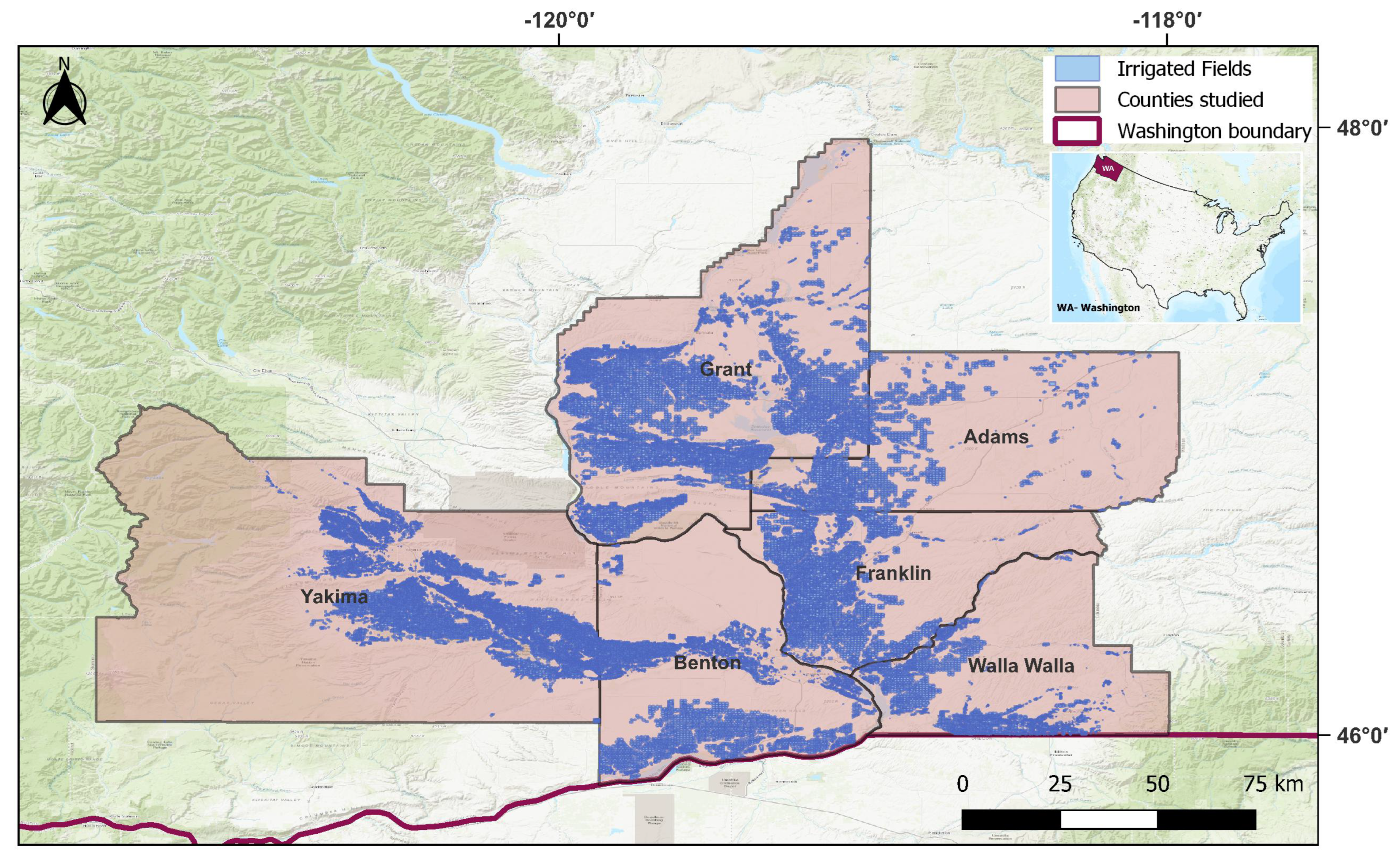
Figure 2.
The overall workflow used for classifying the fields from fetching the data to the final classification approaches is provided here. First we read satellite images on GEE, then compute VIs, then remove noise and smooth their time-series. These steps are followed by creation of ground-truth dataset, and finally we train ML methods to classify them.
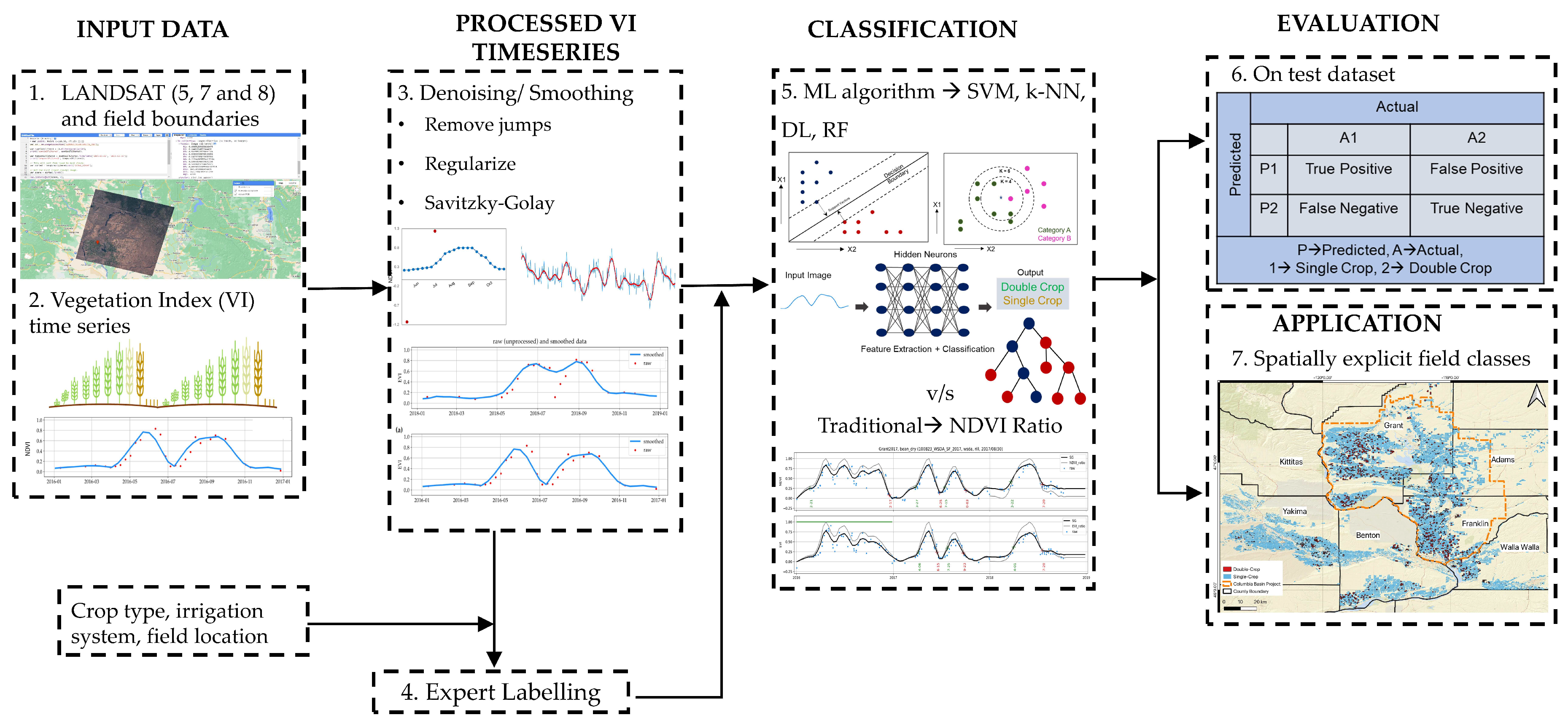
Figure 3.
Training and test sets both cover entire region of interest. They are geographically from the same distribution. Fields in the train set are colored by yellow and test set is presented by red color. This figure shows one of the splits out of six. All splits are shown in Figure A1.
Figure 3.
Training and test sets both cover entire region of interest. They are geographically from the same distribution. Fields in the train set are colored by yellow and test set is presented by red color. This figure shows one of the splits out of six. All splits are shown in Figure A1.
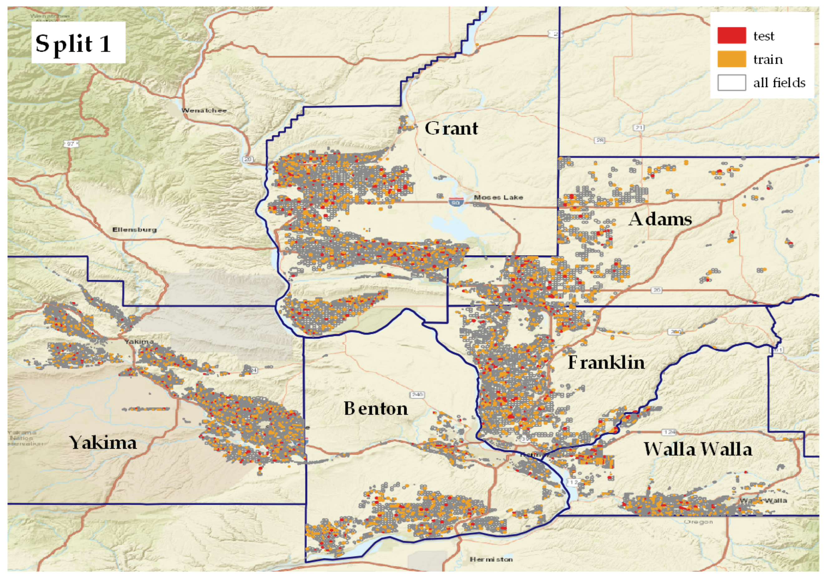
Figure 4.
Examples of raw and smoothed time-series from each group in the confusion matrix for the DL column of Table 3.
Figure 4.
Examples of raw and smoothed time-series from each group in the confusion matrix for the DL column of Table 3.
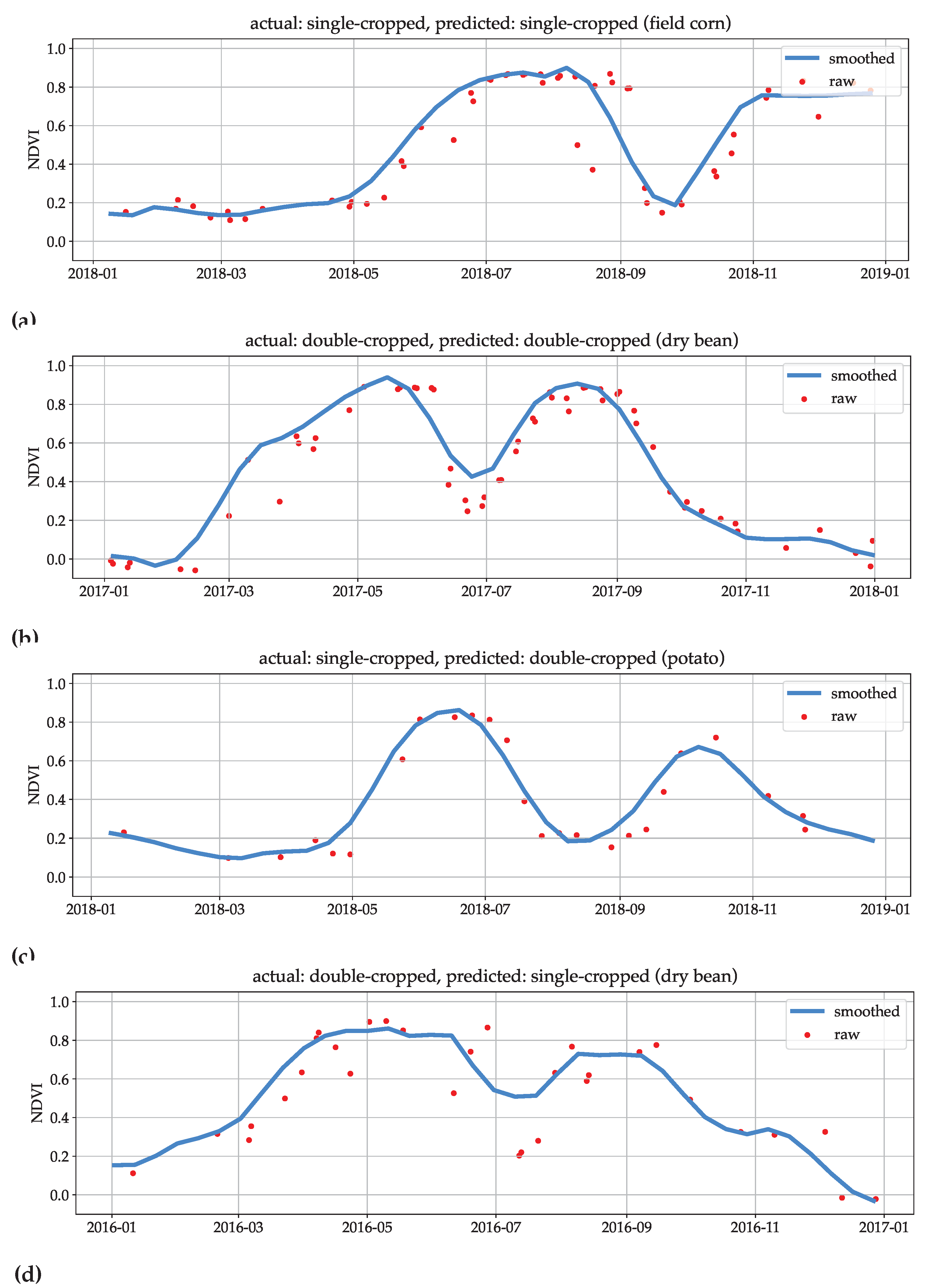
Figure 5.
Fraction (in %) of each crop’s acreage that is classified as a double-cropped. This is based on the test dataset. Perennial crops such as apples, that cannot be double-cropped would have bar heights very close to zero are not displayed in this figure for visual clarity.
Figure 5.
Fraction (in %) of each crop’s acreage that is classified as a double-cropped. This is based on the test dataset. Perennial crops such as apples, that cannot be double-cropped would have bar heights very close to zero are not displayed in this figure for visual clarity.
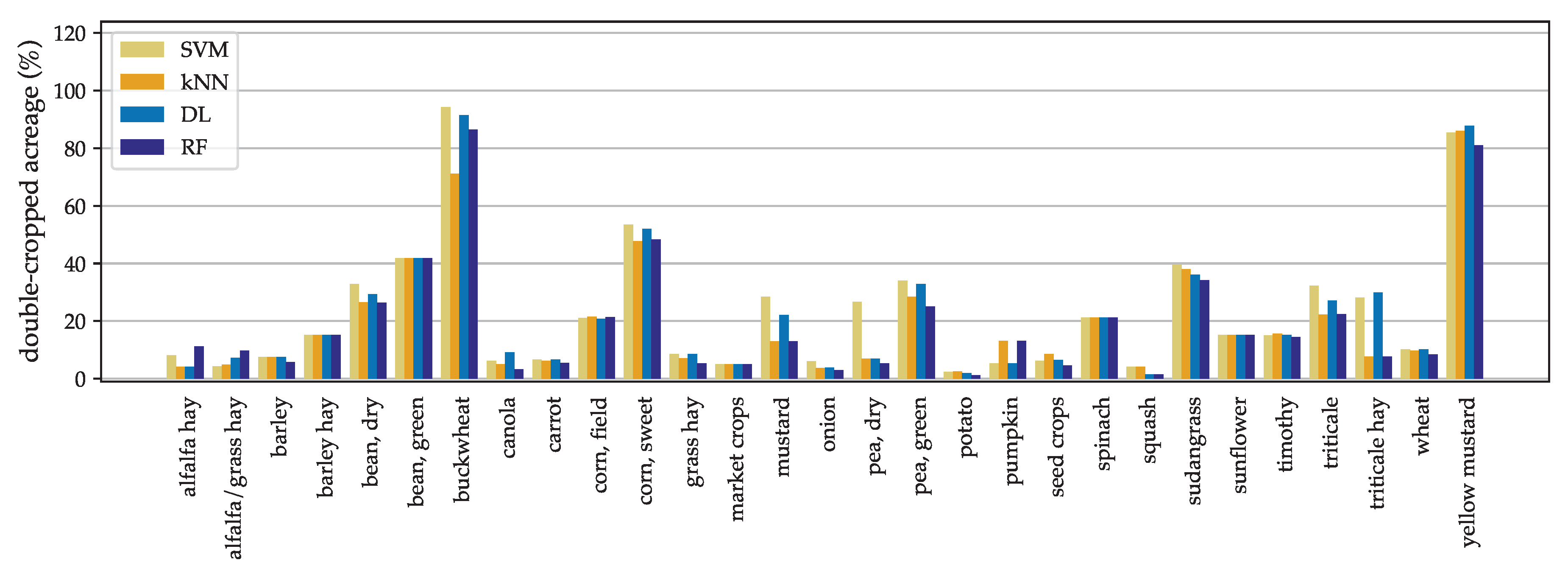
Figure 6.
Spatial distribution of classes of fields is presented in this figure along side the double-cropped area as percentage in each of the counties.
Figure 6.
Spatial distribution of classes of fields is presented in this figure along side the double-cropped area as percentage in each of the counties.

Table 1.
Field boundaries filtered for the different counties based on the surveyed date.
| county | Adams | Benton | Franklin | Grant | Walla Walla | Yakima |
|---|---|---|---|---|---|---|
| survey year | 2016 | 2016 | 2018 | 2017 | 2015 | 2018 |
Table 2.
Crop varieties in the ground-truth set used for training the models. The pair of numbers for each crop indicate the number of fields and the total area in acres, respectively.
Table 2.
Crop varieties in the ground-truth set used for training the models. The pair of numbers for each crop indicate the number of fields and the total area in acres, respectively.
| alfalfa hay (43 - 2,564) | fescue seed (9 - 533) | poplar (44 - 2,445) |
|---|---|---|
| alfalfa seed (23 - 1,274) | grape, juice (71 - 1,926) | potato (185 - 14,989) |
| apple (543 - 13,370) | grape, wine (128 - 3,603) | pumpkin (9 - 272) |
| apricot (16 - 326) | grass hay (46 - 1,492) | ryegrass seed (8 - 513) |
| asparagus (23 - 1,150) | grass seed (34 - 2,039) | sod farm (15 - 796) |
| barley (11 - 575) | hops (120 - 3,040) | squash (9 - 450) |
| barley hay (12 - 636) | market crops (10 - 181) | sudangrass (37 - 1,704) |
| bean, dry (71 - 3,482) | medicinal herb (8 - 225) | sugar beet (10 - 748) |
| bean, green (44 - 1,989) | mint (34 - 1,485) | sugar beet seed (17 - 1,430) |
| blueberry (24 - 1,004) | mustard (2 - 138) | sunflower (7 - 387) |
| bluegrass seed (42 - 3,958) | nectarine/peach (18 - 467) | sunflower seed (29 - 1,185) |
| buckwheat (41 - 2,695) | oat hay (5 - 104) | timothy (70 - 4,848) |
| canola (27 - 2,568) | onion (44 - 3,108) | triticale (18 - 862) |
| carrot (45 - 2,687) | onion seed (8 - 333) | triticale hay (17 - 538) |
| carrot seed (17- 644) | orchard, unknown (9 - 287) | watermelon (10 - 462) |
| cherry (106 - 2,350) | pasture (141 - 4,403) | wheat (207 - 14,151) |
| corn seed (16 - 516) | pea seed (1 - 15) | wheat fallow (42 - 3,239) |
| corn, field (316 - 16,558) | pea, dry (26 - 1,180) | wildlife feed (27 - 1,065) |
| corn, sweet (61 - 4,975) | pea, green (40 - 3,248) | yellow mustard (20 - 1,622) |
| fallow (31 - 692) | pear (31 - 594) | |
| fallow, idle (22 - 528) | pepper (4 - 297) | |
| fallow, tilled (21 - 837) | plum (4 - 64) |
Table 3.
Classification results from the test sets. The ranges correspond to values from the six test sets. User’s and producer’s accuracies reported in this table are for double-cropped class. Table A1 in the Appendix A have the results separated by each test set.
Table 3.
Classification results from the test sets. The ranges correspond to values from the six test sets. User’s and producer’s accuracies reported in this table are for double-cropped class. Table A1 in the Appendix A have the results separated by each test set.
| GT | pred. | SVM | DL | kNN | RF | NDVI-R |
|---|---|---|---|---|---|---|
| 1 | 1 | 556 – 563 | 555 – 568 | 554 – 562 | 562 – 571 | 517 – 536 |
| 2 | 2 | 46 – 55 | 49 – 55 | 43 – 48 | 41 – 44 | 43 – 48 |
| 1 | 2 | 10 – 17 | 5 – 18 | 11 – 19 | 2 – 11 | 37 – 56 |
| 2 | 1 | 4 – 13 | 4 – 10 | 11 – 16 | 15 – 18 | 11 – 16 |
| # err | 15 – 30 | 9 – 25 | 25 – 33 | 20 – 29 | 52 – 67 | |
| OA | 95 – 98% | 96 – 99% | 95 – 96% | 95 – 97% | 89 – 93% | |
| UA | 73 – 84% | 74 – 92% | 70 – 80% | 79 – 95% | 46 – 59% | |
| PA | 78 – 92% | 83 – 93% | 73 – 81% | 69 – 75% | 72 – 83% |
Table 4.
Range of parameters for ML models across the 6 splits of ground-truth.
| parameter | SVM | DL | kNN | RF |
|---|---|---|---|---|
| OA | 95 – 98% | 96 – 99% | 95 – 96% | 95 – 97% |
| OA SE | 0.2 – 0.8% | 0.1 – 0.5% | 0.2 – 0.6% | 0.2 – 0.7% |
| UA double | 73 – 84% | 74 – 92% | 70 – 80% | 79 – 95% |
| UA double SE | 2.1 – 5.5% | 1.4 – 5.2% | 3.2 – 5.7% | 2 – 6.4% |
| PA double | 78 – 92% | 83 – 93% | 73 – 81% | 70 – 75% |
| PA double SE | 1.6 – 5.3% | 1.2 – 2.5% | 2.2 – 3.2% | 2.4 – 5.4% |
Disclaimer/Publisher’s Note: The statements, opinions and data contained in all publications are solely those of the individual author(s) and contributor(s) and not of MDPI and/or the editor(s). MDPI and/or the editor(s) disclaim responsibility for any injury to people or property resulting from any ideas, methods, instructions or products referred to in the content. |
© 2024 by the authors. Licensee MDPI, Basel, Switzerland. This article is an open access article distributed under the terms and conditions of the Creative Commons Attribution (CC BY) license (http://creativecommons.org/licenses/by/4.0/).
Copyright: This open access article is published under a Creative Commons CC BY 4.0 license, which permit the free download, distribution, and reuse, provided that the author and preprint are cited in any reuse.


