
Submitted:
12 September 2023
Posted:
14 September 2023
You are already at the latest version
Abstract
Abstract: The two-dimensional Fuzzy Transform was applied in image compression. The quality of the image compressed with this methodis better than that obtained using methods based on fuzzy relation equations and comparable with that of the JPEG method, with better compression execution times. In this paper we propose a variation of the method based on the two-dimensional Fuzzy Transform of image compression, in which the image is first partitioned into blocks and then each block is compressed with the higher compression rate. The advantage of this method consistsinto a greater compression of the image, guaranteeing a high quality of the reconstructed image.The results show that our method is better than the Fuzzy Transform method improving also the quality of the reconstructed image.
Keywords:
F-transform
; F1-transform
; color image compression
; RGB space
; YUV space.
1. Introduction
YUV is a color model used in the NTSC, PAL, and SECAM color encoding systems., describing the color space in terms of a brightness component (the Y band called luma) and the two chrominance components (the U and V bands called chroma).
The YUV model has been used to advantage in image processing; its main advantage is that, unlike the three Red, Green and Blue (RGB) bands, which are equally perceived by the human eye, in YUV space, most of the color image information is contained in the Y band, as opposed to the U and V bands. main applications of the YUV model in image processing, is then the lossy compression of images, which can be performed mainly in the U and V bands, with slight loss of information.
YUV is used in the JPEG color image compression method [1,2] where the Discrete Cousine Transform (DCT) algorithm is executed on the YUV space, sub-sampling and reducing in dynamic range the UV channels in order to balance the reduction of data and the feel of human eyes. In [3] the DCT algorithm is executed in the YUV space for wireless capsule endoscopy application; the results show that the quality of the reconstructed images is better than that obtained by applying the DCT image compression method in the RGB space.
Many authors proposed image compression and reconstruction algorithms applied on the YUV space in order to improve the quality of the reconstructed images.
In [4,5] an image compression algorithm based on fuzzy relation equations is applied in the YUV space to compress color images; the image is divided in blocks of equal sizes, coding the blocks in the UV channels more strongly than the blocks in the Y band. In [6] the Fuzzy Transform technique (for short, F-transform) [7,8] is applied to coding color images in the YUV space; the author show that the quality of color images coded and decoded via F-transform in the YUV space is better than the one obtained using the F-transform method in the RGB space and comparable with the one obtained using the JPEG method.
A fractal image compression technique applied on the YUV space is proposed in [9]; the authors show that the quality of color images coded/decoded using this approach is better than the one obtained applying the fractal image compression method in the RGB space.
Furthermore, comparison tests between RGB and YUV perception-oriented properties performed in [10] show that compressed images in the YUV space provide better quality than images compressed in the RGB spaces in a human-computer interaction and machine vision applications.
In [11] is applied a technique using Tchebichef bit allocation to compress images in the YUV space; the results shown that this method improves the visual quality of color images compressed via JPEG by 42%. A color image compression method applying a subsampling process to the two chroma channels and a modification algorithm to the Y channel is applied to color images in [12] to improve the JPEG performances.
An image compression method with learning-base filter is applied in [13] on color images constructing the filter in YUV space instead of RGB space; author shows that the quality of the coded images is better than the one obtained using the filter in the RGB space. In [14] an image lossy compression algorithm in which quantization and subsampling are executed in the YUV space is applied for wireless capsule endoscopy; the quality of the coded images results better than the one obtained executing quantization and subsampling in the RGB space. In [15] a wavelet-based color image compression method using trained convolutional neural network are used in the lifting scheme is applied on the YUV executing the trained CNN on the Y, U, V channels separately; this method improves the quality of the coded images obtained applying traditional wavelet-based color image compression algorithms; however, execution times are much higher than those adopted by applying traditional color image compression algorithms.
In [16] an image reconstruction method performed on the YUV space is applied to prevent from corruption of data performed using adversarial perturbation of the image; the results show that the image can be recovered on the YUV space without distortions and with a high visual quality.
In this paper we propose a novel image compression algorithm in which the bidimensional First-Degree F-Transform algorithm [17,18] is applied for coding/decoding color images in the YUV space.
A generalization of the F-transform, called high order Fm-transform, has been proposed in [19] in order to reduce the approximation error of the original function approximated with the inverse F-transform. In the Fm -transform the components of the direct high order fuzzy transforms consist of polynomials of degree s, unlike the components of the direct F-transform (labelled as F°-transform), where they were constant values. The greater the degree of the polynomial, the smaller the error of the approximation; however, as the degree of the polynomial increases, the computational complexity of the algorithm increases.
In [18] the bi-dimensional first-order degree F-transform (F1-transform) is used to compress images; authors show that the quality of the coded/decoded images is better than the one obtained executing F-transform, with negligible augments in CPU time. The critical point of this method consists of the fact that, unlike the F-transform and JPEG methods, it requires not the compressed image to be saved in memory, but matrices of three coefficients of the same size as the compressed image; therefore, it needs a memory area three times greater than that necessary to archive the compressed image.
To solve this problem, we propose a new lossy color image compression algorithm in which is executed the F1-transform algorithm to code/decode color images transformed in the YUV space. The transformed image in each of the three channels is partitioned into blocks and each block is compressed by the bi-dimensional direct F1-transform, compressing the blocks of the chroma channels more. The image is subsequently reconstructed by decomposing the single blocks with the use of the bi-dimensional inverse F1-transform.
The main benefits of this method are as follows:
- the use of the bi-dimensional F1-transform represents a trade-off between the quality of the compressed image and the CPU times. It reduces the information loss obtained by compressing the image with the same compression rate using the F-transform algorithm with acceptable coding/decoding CPU time;
- the compression of the color images is carried out in the YUV space to guarantee a high visual quality of the color images and solve the criticality of the F1-transform color image compression method on the RGB space [18] which needs a larger memory to allocate the information of the compressed image. In fact, by performing a high compression of the two chrominance channels, the size of the matrices in which the information of the compressed image is contained, is reduced in these two channels, and this allows to reduce the memory allocation and CPU times.
We compare our color lossy image compression method with the JPEG method and with the image compression methods based on the bi-dimensional F-transform [7,8] and F1-transform [19] on the RGB space and on the bi-dimensional F-transform on the YUV space [6].
In the next Section the concepts of F-transform and F1-transform are briefly presented, and the F-transform lossy color image compression method applied in YUV space is shown as well. Our method is presented in Section 3. In Section 4 the comparative results obtained on datasets of color images are shown and discussed; concluding discussions are contained in Section 5.
2. Preliminaries
2.1. The bi-dimensional F-Transform
Let [a,b] be a closed real interval and let {x1, x2, …, xn} be a set of points of [a,b], called nodes, such that x1 = a < x2 <…< xn = b.
Let {A1,…,An} be a family of fuzzy sets of X, where Ai : [a,b] → [0,1: it forms a fuzzy partition of X if the following conditions hold:
(1) Ai(xi) = 1 for every i =1,2,…,n;
(2) Ai(x) = 0 if x∉(xi-1, xi+1), by setting x0 = x1 = a and xn+1 = xn = b;
(3) Ai(x) is a continuous function over [a,b];
(4) Ai(x) is strictly increasing over [xi-1, xi] for each i = 2, …, n ;
(5) Ai(x) is strictly decreasing over [xi, xi+1] for each i = 1,…, n-1;
(6) for every x∈[a,b].
Let . The fuzzy partition {A1,…, An} is an uniform fuzzy partition if:
(7) n≥3;
(8) xi =a+h∙(i-1), for every i = 1, 2, …, n;
(9) Ai(xi – x) = Ai(xi + x) for every x [0,h] and i = 2,…, n-1;
(10) Ai+1(x) = Ai(x - h) for every x [xi, xi+1] and i = 1,2,…, n-1.
Let f(x) be a continuous function over [a,b] and {A1, A2, …, An} be a fuzzy partition of [a,b]. The n-tuple F = is called unidimensional direct F-transform of f with respect to {A1, A2, …, An} if the following hold:
The following function defined in [a,b]:
is called uni-dimensional inverse F-transform of the function f.
The following theorem holds (cfr. [7, Theorem 2]):
Theorem 1.
Let f(x) be a continuous function over [a,b]. For every ε > 0 there exist an integer n(ε) and a fuzzy partition {A1, A2, …, An(ε)} of [a,b] such that for all x[a, b].
Now consider the discrete case where the function f is known in a set of N points P = {p1,...,pN}, where pj∈[a,b] j = 1,2,…,m. The set {p1,...,pN} is called sufficiently dense with respect to the fixed fuzzy partition {A1, A2, …, An} if for every i = 1,…,n, there exists at least an index j{1,…,m} such that Ai(pj) > 0.
If the set P is sufficiently dense with respect to the fuzzy partition, we can define the discrete direct F-transform with components:
and the discrete inverse F-transform:
The following theorem applied to the discrete inverse F-transform holds (cfr. [7, Theorem 5]):
Theorem 2.
Let f(x) be a continuous function over [a,b], known in a discrete set of points {p1,...,pm}. For every ε > 0 there exist an integer n(ε) and a fuzzy partition {A1, A2, …, An(ε)} of [a,b], with respect to which P is sufficiently dense, that is such that for every j = 1,…,N,.
By Theorem 2, the inverse fuzzy transform (4) can be used to approximate the function f in a point.
Now we consider functions in two variables. Let x1, x2, …, xn be a set of n nodes in [a,b] , where n > 2 and x1 = a < x2 <…< xn = b, and let y1, y2, …, ym be a set of n nodes in [c,d], where m > 2 and and y1 = c < y2 <…< ym = d. Moreover, let A1,…,An : [a,b] → [0,1] be a fuzzy partition of [a,b], B1,…,Bm : [c,d] → [0,1] be a fuzzy partition of [c,d] and let f(x,y) be a function defined in the closed set [a,b]×[c,d].
We suppose that f assumes known values in a set of points (pj,qj) ∈[a,b]×[c,d], where i = 1,…,N and j = 1,…,M, where the set P={p1, … , pN} is sufficiently dense with respect to the fuzzy partition {A1,…, An} and the set Q={q1, … ,qM} is sufficiently dense with respect to the fuzzy partition {B1,…,Bm}.
In this case, we can define the bi-dimensional discrete F-transform of f, given by matrix [Fhk] h = 1,…,n and k = 1,…,m with components:
and the bi-dimensional discrete inverse F-transform of f with respect to {A1, A2, …, An} and {B1,…,Bm} given by
2.2. The bi-dimensional F1-Transform
This paragraph introduces the concept of higher degree fuzzy transform or Fr-transform. One-dimensional square-integrable functions will now be considered.
Let Ah, h = 1,…,n, be the hth fuzzy set of the fuzzy partition {A1,…,An} defined on [a,b] and L2([xh−1,xh+1]) be the Hilbert space of square-integrable functions f,g: [xh−1,xh+1] ⟶ R with the inner product:
Given a positive integer r, we denote with ([xh−1,xh+1]) a linear subspace of the Hilbert space L2([xh−1,xh+1]) having as orthogonal basis the polynomials {, ,…,} constructed applying the Gram-Schmidt ortho-normalization defined as:
The following Lemma holds (Cfr. 7, Lemma 1):
Lemma 1.
Let be the orthogonal projection of the function f on ([xh−1,xh+1]). Then:
where
it is the hth component of the direct Fr-transform of f . The inverse Fr-transform of f in a point x ∊ [a,b] is:
For r = 0, we have = 1 and the F0-transform is given by the F-transform in one variable ((x) = ch,0).
For r = 1, we have (x) = (x − xh) and the hth component of the F1-transform is given by the formula:
If the function f is known in a set of N points P ={p1,…pN}, ch,0 and ch,1 can be discretized in the form:
The F1-tranform can be extended in a bi-dimensional space. Let L2 ([xh−1, xh+1] × [yk−1, yk+1]) be the Hilbert space of square- integrable functions f: [xh−1, xh+1] × [yk−1,yk+1]→ R with the weighted inner product:
Two functions L2 ([xh−1, xh+1] × [yk−1, yk+1]) are orthogonal if .
Let f: X ⊆ R2 → Y⊆ R be a continuous bi-dimensional function defined in a closed set [a,b] × [c,d]. Let {A1, A2,…, An} be a fuzzy partition of [a,b], and let {B1, B2,…, Bm} be a fuzzy partition of [c,d].
Moreover, let {(p1,q1),…, (pN,qjN)} a set of N points in which is known the function f, where (pj,qj) [a,b]×[c,d]. Let the set P={p1, … , pN} be sufficiently dense with respect to the fuzzy partition {A1,…, An} and let the set Q={q1, … ,qM} be sufficiently dense with respect to the fuzzy partition {B1,…,Bm}.
We can define the bi-dimensional direct F1-transform of f, with components:
where is the component of the bi-dimensional discrete direct F transform of f, given by (5). The three coefficients in (17) are given by:
The inverse F1-transform of f in a point (x,y) ∊ [a,b] × [c,d] is:
where is the (h,k)th component of the bi-dimensional direct F1-transform, given by the formula (16).
2.3. Coding/decoding images using the bi-dimensional F and F1-Transforms
Let I be a grey N × M image. A pixel can be considered a data point with coordinates (i,j), where i = 1,2,…,N and j = 1,2,…M; the value of this data point is given by the pixel value I(i,j). In [8] the image is normalized in [0,1] according with the formula R(i,j) = I(i,j)/(L-1) where L is the number of grey levels, partitioned in blocks of equal sizes N(B)×M(B), coded to a block FB of sizes n(B) × m(B) with n(B) << N(B) and m(B) << M(B), using the bi-dimensional direct F-transform.
Let {A1,…,An(B)} be a fuzzy partition of [1,N(B)] and let {B1,…,Bm(B)} be a fuzzy partition of [1,M(B))], each block is compressed by the bi-dimensional direct F-transform:
The coded image is reconstructed by merging all compressed blocks.
Each block is decompressed by using the bi-dimensional inverse F-transform. The pixel value I(i,j) in the block is approximated by the value:
The decoded image is reconstructed by merging the decompressed blocks.
The F-transform compression and decompression algorithms are shown in pseudocode in Algorithms 1a and 1b.
| Algorithm 1a. F1-transform image compression |
|
Input: N×M Image I with L grey levels Size of the blocks of the source image N(B)×M(B) Size of the compressed blocks n(B)× m(B) |
| Output: n×m compressed image IC |
|
| Algorithm 1b. F-transform image decompression |
| Input: n×m compressed image Ic |
| Output: N×M decoded image ID |
|
In [17] an improvement of the quality of the decompressed image is accomplished using the bi-dimensional F1-transform.
The blocks are compressed by using the bi-dimensional direct F1-transform:
where:
The above three coefficients are constructed merging the coefficients of each block and finally stored, forming the output of coding process.
In the inverse process the image is reconstructed by decompressing the block with the bi-dimensional inverse F1-transform:
where the bi-dimensional direct F1-transform of the block is calculated by (23).
The decompressed blocks are merged to form the decompressed image.
The F1-transform compression and decompression algorithms are shown in pseudocode in Algorithms 2a and 2b.
| Algorithm 2a. F1-transform image compression |
|
Input: N×M Image I with L grey levels Size of the blocks of the source image N(B)×M(B) Size of the compressed blocks n(B)× m(B) |
| Output: n×m matrices of the direct F1-transform coefficients |
|
| Algorithm 2b. F1-transform image decompression |
|
Input: n×m matrices of the direct F1-transform coefficients coefficients Size of the blocks of the decoded image N(B)×M(B) Size of the blocks of the coded image n(B)×m(B) |
| Output: N×M decoded image ID |
|
3. The YUV-based F1-transform color image compression method
Let I be a N×M color image in L grey levels. All pixel values in the three bands R, G and B are normalized in [0,1].
Considering a 256 grey levels color image and the scaled and offset version of the YUV color space, the source image is transformed in the YUV space via the formula [20]:
Then, the F1-transform image compression algorithm is executed separately to the three normalized images Y, U and V, using a strong compression for the chroma images U and V.
If N(B) and M(B) are the sizes of each block in the three channels, the blocks in the brightness channel are compressed with rate and the blocks in the two chroma channels are compressed with rate , where nUV(B) << nY(B) and mUV(B) << mY(B), so that ρUV << ρY .
The F1-transform image compression algorithm will store, in output for each channel, the three matrixes of the coefficients of the bi-dimensional direct F1-transform: , and . The size of the three matrices in the brightness channel is ρY(N×M) and the size of the three matrices in each of the two chroma channels is ρUV(N×M).
By suitably choosing the brightness and chroma compression rates, it is possible to reduce the memory capacity needed to store the direct F1-transform coefficients in the RGB space.
For example, suppose we execute the F1-transform image compression algorithm in the RGB space to compress a 256×256 color image, by partitioning the image into 16x16 blocks compressed into 4×4 blocks. The compression rate will be ρRGB = 0.0625 and the size of the matrix of each coefficient is 64×64. Executing the F1-transform algorithm in the YUV space and compressing the 16×16 blocks in the two chroma channels in 2×2 blocks (ρUV = 0.016) and the 16×16 blocks in the brightness channel in 8×8 blocks (ρUV = 0.25), the size of the matrix of each coefficient in the U and V channels will be 32×32, and the size of the matrix of each coefficient in the Y channel will be 128×128. So, by carrying out the compression of the source image in the YUV space in this way, an advantage is obtained both in terms of visual quality of the reconstructed image and in terms of available memory necessary to archive the coefficients of the direct F1-transforms in the three channels.
Below we show in pseudocode the YUV F1-transform color image compression algorithm (Algorithm 3a).
| Algorithm 3a. YUV F1-transform color image compression |
|
Input: N×M color image I with L grey levels Size of the blocks of the source image N(B)×M(B) Size of the compressed blocks in the Y channel nY(B)× mY(B) Size of the compressed blocks in the U and V channels nUV(B)×mUV(B) |
| Output: n×m matrices of thedirect F1-transform coefficients in the Y, U and channels |
|
The decompression process is performed by executing the F1-transform image decompression algorithm in the brightness and chroma channels. The F1-transform image decompression algorithm is executed separately for each of the channels Y, U and V, by assigning as input both the three coefficient matrices of the direct F1-transform and the dimensions of the original and compressed blocks.
Then the three decoded images IDY, IDU, and IDV are transformed in the RGB space, by the formula [20]:
Finally, the decoded image in the RGB band (IDR, IDG, IDB) is returned.
Below is shown in pseudocode the YUV F1-transform color image decompression algorithm (Algorithm 3b).
| Algorithm 3b. YUV F1-transform image decompression |
|
Input: n×m matrices of the direct F1-transform coefficients coefficients in the Y, U and V channels Size of the blocks of the decoded image N(B)×M(B) Size of the compressed blocks in the Y channel nY(B)× mY(B) Size of the compressed blocks in the U and V channels nUV(B)×mUV(B) |
| Output: N×M decoded image ID |
|
We compare our lossy color image compression report with the JPEG algorithms and the color image compression methods based on F-transform in the RGB space [8], and F-transform on the YUV space [6] and F1-transform on the RGB space [17].
The Peak Signal to Noise index (PSNR) used to measure the quality of the decoded images. To measure the gain obtained executing the YUV F1-transform algorithm with respect to another color image compression method, we measure the PSNR gain, expressed in percentage and given by the formula
In next Section the results applied to color image dataset are shown and discussed.
4. Results
We test the YUV F1-transform lossy color image compression algorithm on the color image dataset provided by the University of Southern California Signal and Image Processing Institute (USC SIPI) and published on the website http://sipi.usc.edu/database.
The dataset is made up of over 50 color images of different sizes. For brevity, we show in detail the results obtained for the 256x256 source images 4.1.04 and the 412x512 source image 4.2.07; they are shown in Figure 1.
Each image was compressed and decompressed by performing JPEG, YUV F-transform, F1-transform and YUV F1-transform lossy image compression algorithms.
We compare the four image compression methods measuring the quality of the reconstructed image as the compression rate change. The compression rate used by executing YUV F-transform and YUV F1-transform is the mean compression rate set for each channel Y, U and V.
In Figure 2 we show, for the original image 4.1.04, the decoded images obtained by executing the four algorithms with a compression rate ρ ≈ 0.10.
Figure 3 shows, for the original image 4.1.04, the decoded images obtained by executing the four algorithms setting a compression rate ρ ≈ 0.25.
Figure 4 shows the trend of the PSNR index obtained varying the compression rate. The trends obtained by executing JPEG and F1-transform are similar. However, for strong compressions (ρ < 0.1), the PSNR value calculated by executing JPEG decreases exponentially as the compression increases: this result shows that the quality of the decoded image obtained by JPEG drops quickly for very high compressions. The highest PSNR values are obtained by performing YUV F-transform and YUV F1-transform. In particular, the PSNR values obtained with the two methods are similar for ρ < 0.2, while, for lower compressions, YUV F1-transform provides decompressed images of better quality than those obtained with YUV F-transform.
Now we show the results obtained for the color image 4.2.07. In Figure 5 we give the decoded images obtained by executing the four algorithms with compression rate ρ ≈ 0.10.
Figure 6 shows the decoded images of 4.2.07 obtained by executing the four algorithms with a compression rate ρ ≈ 0.25.
Figure 7 shows the trend of the PSNR index obtained by varying the compression rate. The best values of PSNR are obtained by executing YUV F1-transform. The trend of the PSNR obtained by executing YUV F-transform is better than the one obtained by executing F-transform and JPEG. As the results obtained for the color image 4.1.04 show, the trend of PSNR obtained by executing JPEG for the image 4.2.07 decays rapidly as compression increases (ρ < 0.1).
In Figure 8 we show the trends of the gain of the YUV F1-transform algorithm with respect to the other three color image compression algorithms, where the gain index is calculated by (30) and is averaged for all the images of the dataset used in the comparative tests. The gain of the proposed method with respect to YUV F-transform is approximately equal to 2% regardless of the compression rate. The gain of YUV F1-transform with respect to F1-transform varies from 3%, for small compressions, to 4% for high compressions (ρ < 0.2). The gain of YUV F1-transform with respect to JPEG varies from 3%, for small compressions, to 5% for medium-high compressions (0.1 < ρ < 0.2); for compression rates lower than 0.1 the gain index increases quickly as the compression increases until it reaches 7%.
These results shown that the quality of the images coded/decoded by YUV-F1transform is higher than that obtained using YUV-Ftransform, F1transform and JPEG, regardless of the compression level.
Finally, in Table 1 we show the mean coding and decoding CPU time obtained by executing the four color image compression algorithms: the average values refer to the CPU times measured for all images of the same size and for all compression rates: we see that both the coding and decoding CPU times measured by executing YUV F1-transform are comparable with those obtainedwith the other four image compression methods. Therefore, YUV-F1-transform improves the quality of the reconstructed images obtained by executing JPEG, F1-transform and YUV F-transform and provides CPU times similar to those obtained by executing the other image compression three methods at same time.
5. Conclusions
A lossy color image compression process employing the bi-dimensional F1-transform in YUV space is proposed. The benefit of this approach is to improve the quality of the reconstructed image, with acceptable CPU coding/decoding times. In fact, the F1-transform method manages to retain more information of the original image than other image compression methods, but with memory to be allocated and execution times. The proposed method on the YUV space allows to obtain a high quality of the decompressed image, without increasing the allocated memory and the CPU times. The results show that this method improves the quality of the decompressed image compared to that obtained with the use of JPEG, F-transform applied in YUV space and F1-transform applied in RGB space. Moreover the execution times are compatible with those obtained by executing the other three color image compression methods.
In the future we intend to adapt the YUV F1-transform algorithm to the compression of large color images
Author Contributions
Conceptualization, B. C.. and S.S.; methodology, B. C., F.D.M. and S.S.; software, B. C., F.D.M. and S.S.; validation, B. C., F.D.M. and S.S.; formal analysis, B. C., F.D.M. and S.S.; investigation, B. C., F.D.M. and S.S.; resources, B. C., F.D.M. and S.S.; data curation, B. C., F.D.M. and S.S.; writing—original draft preparation, B. C., F.D.M. and S.S.; writing—review and editing, B. C., F.D.M. and S.S.; visualization, B. C., F.D.M. and S.S.; supervision, B. C., F.D.M. and S.S.
Funding
This research received no external funding.
Conflicts of Interest
The authors declare no conflict of interest.
References
- Wallace, G. The JPEG still picture compression standard. IEEE Transactions on Consumer Electronics 1992, 38(1), xviii–xxxiv. [CrossRef]
- Raid, A. M.; Khedr, W. M.; El-Dosuky, M. A.: Ahmed, W. Jpeg image compression using discrete cosine transform-A survey. International Journal of Computer Science & Engineering Survey (IJCSES) 2014, 5(2), 39-47. [CrossRef]
- Mostafa, A.; Wahid, K.; Ko, S.B. An Efficient YUV-based Image Compression Algorithm for Wireless Capsule Endoscopy, IEEE CCECE 2011 2011 24th Canadian Conference on Electrical and Computer Engineering (CCECE) 8-11 May 2011, Niagara Falls, Ontario, Canada., pp 943-946. [CrossRef]
- Nobuhara, H.; Pedrycz, W.; Hirota, K. Relational image compression: optimizations through the design of fuzzy coders and YUV color space, Soft Computing 2005, 9(6), 471–479. [CrossRef]
- Nobuhara, H.; Hirota, K.; Di Martino, F.; Pedrycz, W.; Sessa S. Fuzzy relation equations for compression/decompression processes of colour images in the RGB and YUV colour spaces, Fuzzy Optimization and Decision Making 2005, 4(3), 235–246. [CrossRef]
- Di Martino, F.; Loia, V.; Sessa, S. Direct and Inverse Fuzzy Transforms for Coding/Decoding Color Images in YUV Space, Journal of Uncertain Systems 2009, 3(1), 11-30.
- Perfilieva, I. Fuzzy Transform: Theory and Application. Fuzzy Sets and Systems 2006, 157, 993-1023. [CrossRef]
- Di Martino, F.; Loia, V.; Perfilieva, I.; Sessa, S. An Image Coding/Decoding Method Based on Direct and Inverse Fuzzy Transforms. International Journal of Approximate Reasoning 2008, 48, 110-131. [CrossRef]
- Son, T. N.; Hoang, T. M.; Dzung, N. T.; Giang, N. H. Fast FPGA implementation of YUV-based fractal image compression, 2014 IEEE Fifth International Conference on Communications and Electronics (ICCE), Danang, Vietnam, 2014, pp. 440-445. [CrossRef]
- Podpora, M.; Korbas, G. P.; Kawala-Janik, A. YUV vs RGB – Choosing a Color Space for Human-Machine Interaction, 2014 Federated Conference on Computer Science and Information Systems, Warsaw, Poland, 7 - 10 September 2014, vol. 3 pp. 29–34. [CrossRef]
- Ernawan, F.; Kabir, N.; Zamli, K.Z., An efficient image compression technique using Tchebichef bit allocation. Optik, 2017, 148, 106-119.
- Zhu, S.; Cui, C.; Xiong, R.; Guo, U.; Zeng, B. Efficient Chroma Sub-Sampling and Luma Modification for Color Image Compression, in IEEE Transactions on Circuits and Systems for Video Technology, vol. 29, no. 5, pp. 1559-1563, May 2019. [CrossRef]
- Sun, H.; Liu, C.; Katto, J.; Fan, Y. An Image Compression Framework with Learning-Based Filter, Proceedings of 2020 IEEE/CVF Conference on Computer Vision and Pattern Recognition Workshops (CVPRW), 14-19 June 2020, Seattle, WA, USA, pp. 152-153.
- Malathkar, N.V.; Soni, S.K. High compression efficiency image compression algorithm based on subsampling for capsule endoscopy. Multimed Tools Appl 2021, 80, 22163–22175. [CrossRef]
- Ma, H.; Liu, D.; Yan, N.; Li, H.; Wu, F. End-to-End Optimized Versatile Image Compression With Wavelet-Like Transform IEEE Transactions on Pattern Analysis and Machine Intelligence 2022, 44, (3),. 1247-1263. [CrossRef]
- Yin, Z.; Chen, L.;Lyu, W.;Luo, B. Reversible attack based on adversarial perturbation and reversible data hiding in YUV colorspace. Pattern Recognition Letters 2023, 166, 1-7. [CrossRef]
- Di Martino, F.; Sessa, S.; Perfilieva, I. First Order Fuzzy Transform for Images Compression. Journal of Signal Information Processing 2017, 8, 178-94. [CrossRef]
- Di Martino, F.; Sessa, S. Fuzzy Transforms for Image Processing and Data Analysis - Core Concepts, Processes and Applications; Springer Nature: Cham, Switzerland, 2020, pp. 217. [CrossRef]
- Perfilieva, I.; Dankova, M.; Bede, B. Towards a higher degree F-transform. Fuzzy Sets and Systems 2011, 180, 3–19. [CrossRef]
- Technical Committee ISO/IEC JTC 1/SC 29 Coding of audio, picture, multimedia and hypermedia information, ISO/IEC 10918-1:1994 - Information technology — Digital compression and coding of continuous-tone still images: Requirements and guidelines, 1994, 182 pp.
- Wang, Y.; Tohidypour, H.R.; Pourazad, M.T.; Nasiopoulo, P.; Leung, V.C.M. Comparison of Modern Compression Standards on Medical Images for Telehealth Applications. In 2023 IEEE International Conference on Consumer Electronics (ICCE), 2023, pp. 1-6.
- Prativadibhayankaram, S.; Richter, T.; Sparenberg, H.; Fößel, S. Color Learning for Image Compression. arXiv preprint arXiv, 2023, 2306.17460.
- Yin, Z.; Chen, L.;Lyu, W.;Luo, B. Reversible attack based on adversarial perturbation and reversible data hiding in YUV colorspace. Pattern Recognition Letters 2023, 166, 1-7. [CrossRef]
Figure 1.
Source images: (a) 256x256 image 4.1.04; (b): 512x512 image 4.2.07.
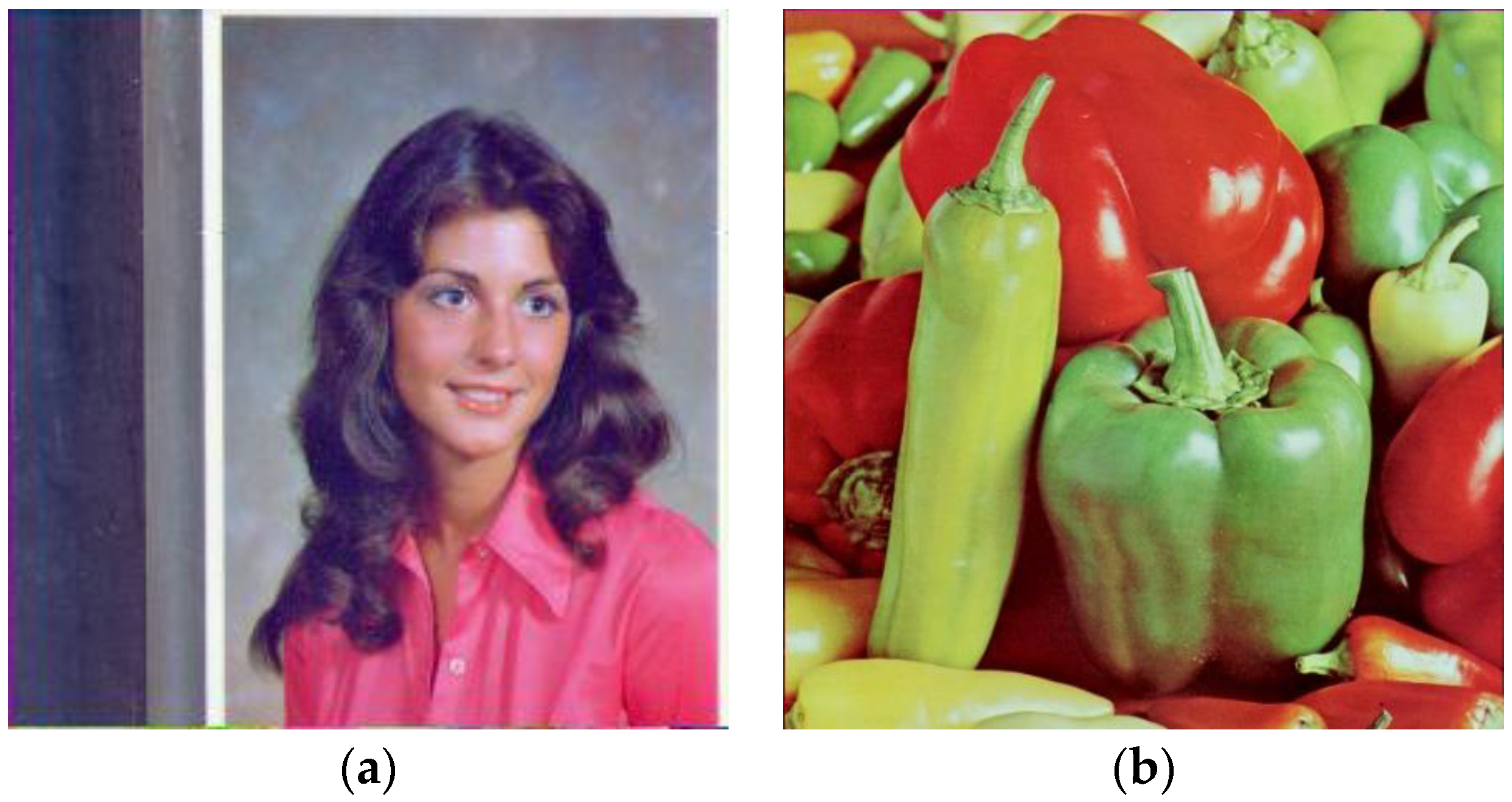
Figure 2.
Decoded image 4.1.04, ρ ≈ 0.10, obtained via: (a) JPEG; (b) F1-transform; (c):YUV F-transform; (d) YUV F1-transform.
Figure 2.
Decoded image 4.1.04, ρ ≈ 0.10, obtained via: (a) JPEG; (b) F1-transform; (c):YUV F-transform; (d) YUV F1-transform.


Figure 3.
Decoded image 4.1.04, ρ ≈ 0.25, obtained via: (a) JPEG; (b) F1-transform; (c):YUV F-transform; (d) YUV F1-transform.
Figure 3.
Decoded image 4.1.04, ρ ≈ 0.25, obtained via: (a) JPEG; (b) F1-transform; (c):YUV F-transform; (d) YUV F1-transform.
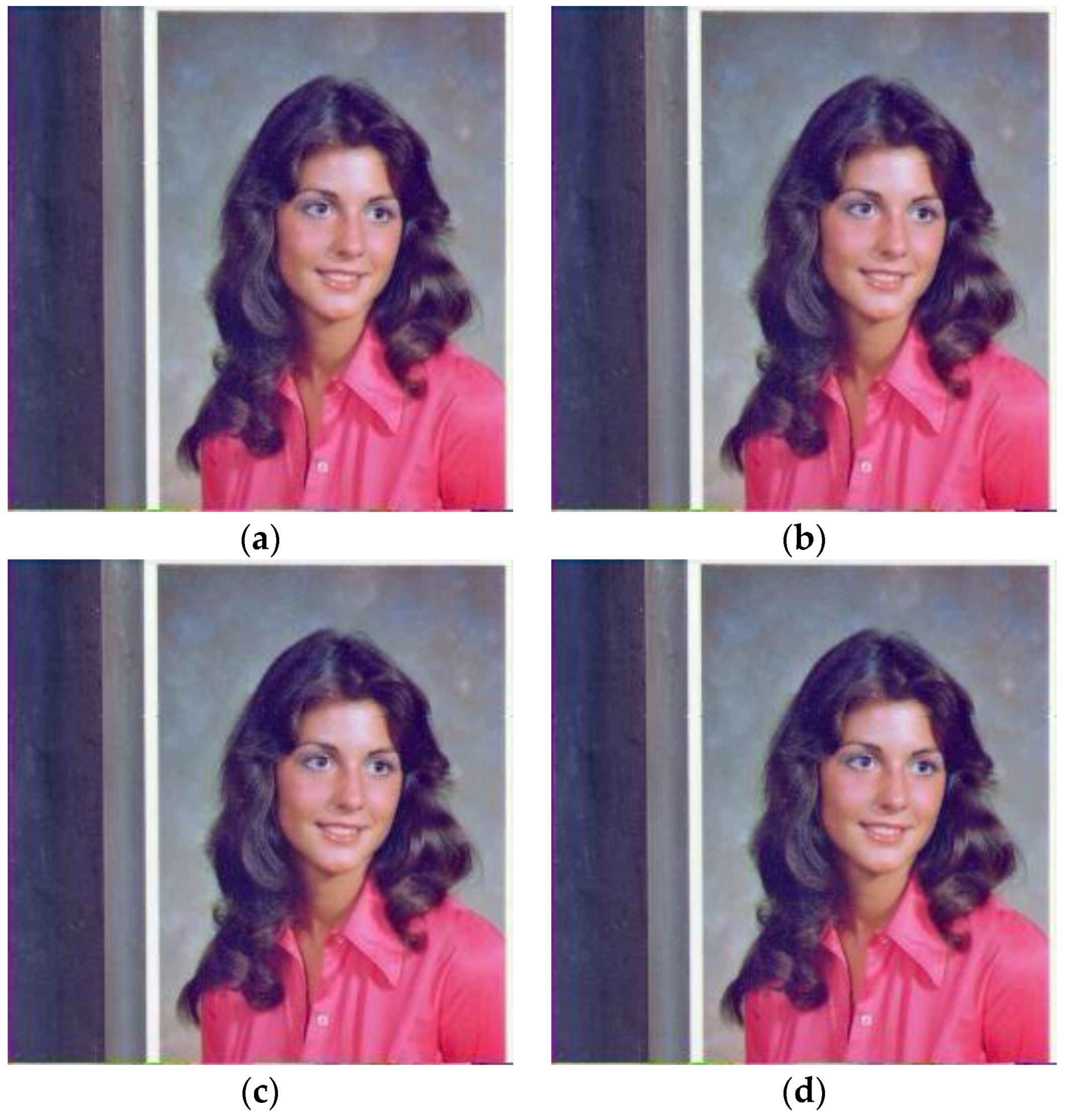
Figure 4.
PSNR trend for the color image 4.1.04 obtained by executing the four color image compressions algorithms.
Figure 4.
PSNR trend for the color image 4.1.04 obtained by executing the four color image compressions algorithms.
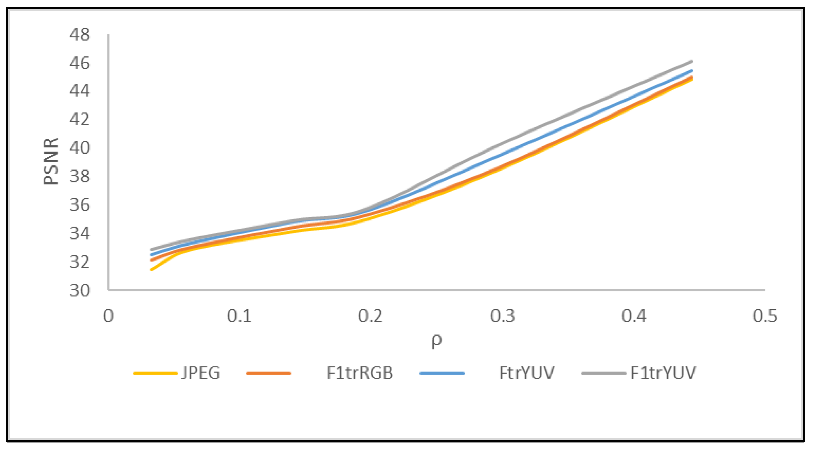
Figure 5.
Decoded image 4.2.07, ρ ≈ 0.10, obtained via: (a) JPEG; (b) F1-transform; (c):YUV F-transform; (d) YUV F1-transform.
Figure 5.
Decoded image 4.2.07, ρ ≈ 0.10, obtained via: (a) JPEG; (b) F1-transform; (c):YUV F-transform; (d) YUV F1-transform.
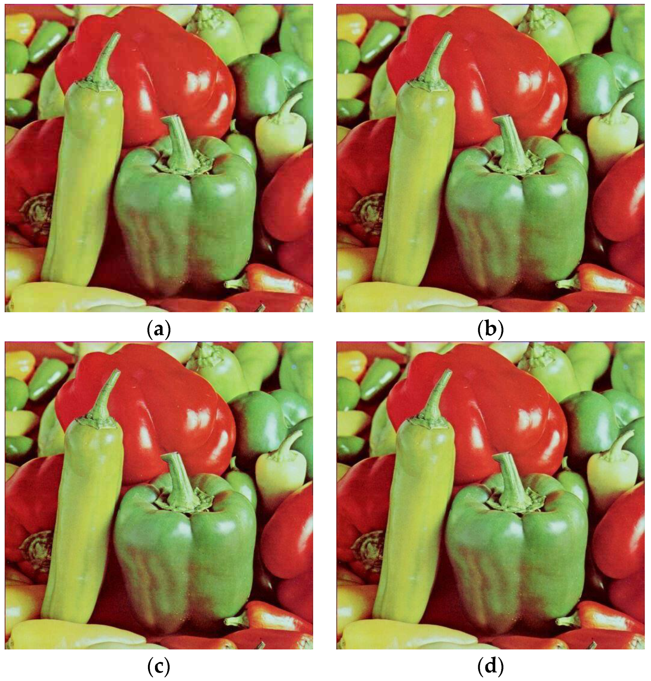
Figure 6.
Decoded image 4.2.07, ρ ≈ 0.25, obtained via: (a) JPEG; (b) F1-transform; (c):YUV F-transform; (d) YUV F1-transform.
Figure 6.
Decoded image 4.2.07, ρ ≈ 0.25, obtained via: (a) JPEG; (b) F1-transform; (c):YUV F-transform; (d) YUV F1-transform.

Figure 7.
PSNR trend for the color image 4.2.07 obtained by executing the four color image compressions algorithms.
Figure 7.
PSNR trend for the color image 4.2.07 obtained by executing the four color image compressions algorithms.
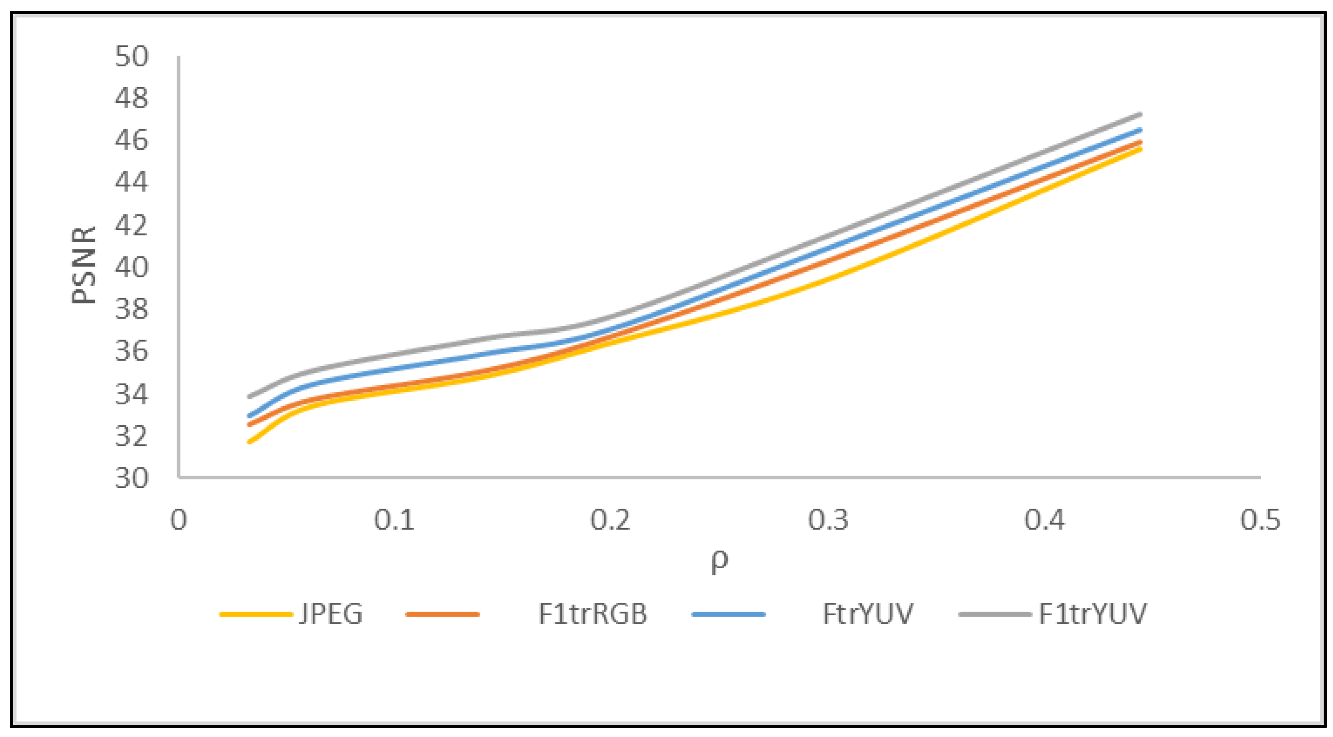
Figure 8.
Trend of the Gain of YUV-F1transform with respect to the other three color image compression methods.
Figure 8.
Trend of the Gain of YUV-F1transform with respect to the other three color image compression methods.
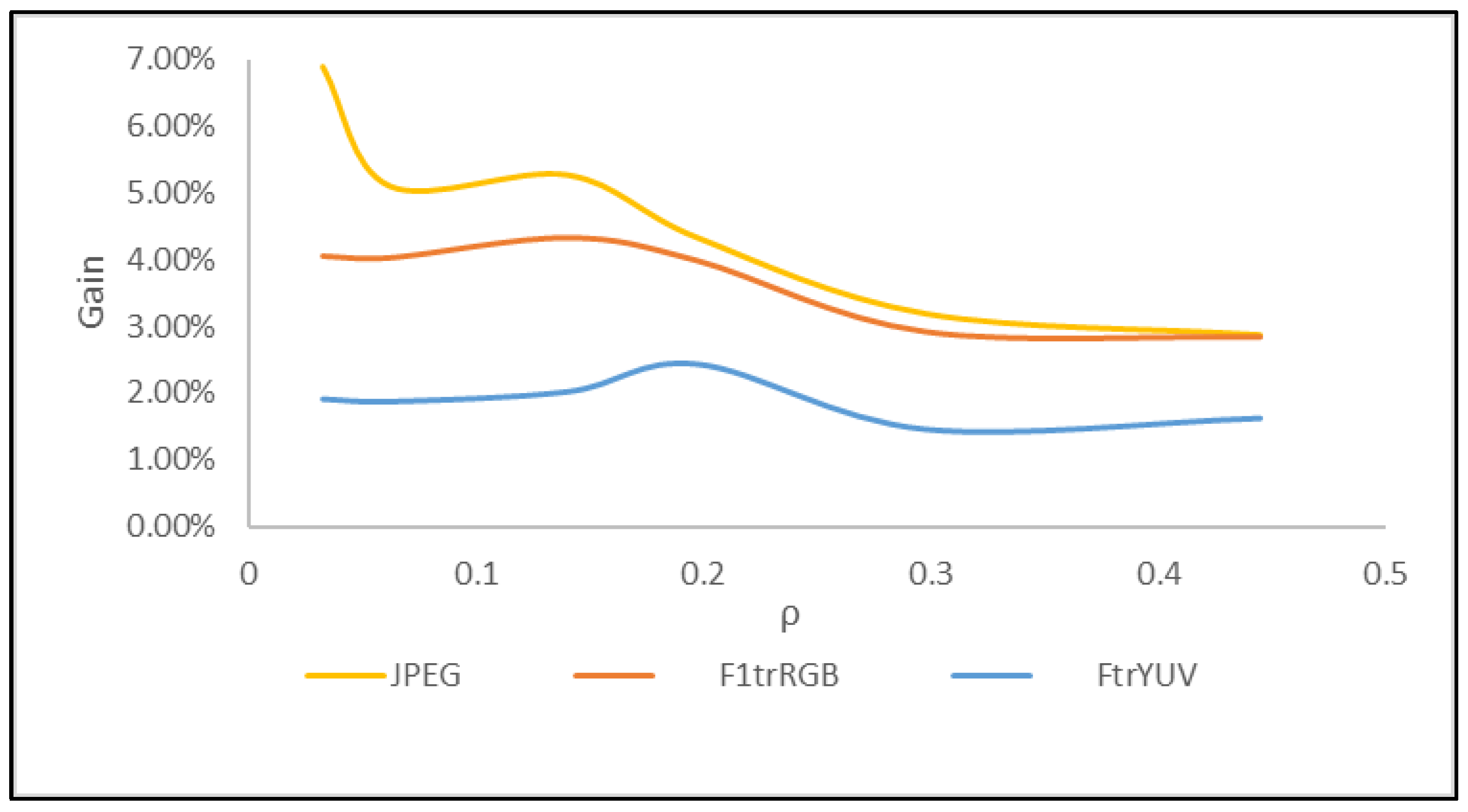

Table 1.
Mean coding and decoding CPU time obtained for the 256x256 and 512x512 images by executing the four image compression algorithms.
Table 1.
Mean coding and decoding CPU time obtained for the 256x256 and 512x512 images by executing the four image compression algorithms.
| CPU time | JPEG | F1trRGB | FtrYUV | F1trYUV | |
|---|---|---|---|---|---|
| Coding | 256x256 | 2.76 | 2.78 | 2.41 | 3.09 |
| 512x512 | 5.75 | 5.88 | 5.66 | 6.01 | |
| Decoding | 256x256 | 5.82 | 5.86 | 5.04 | 5.73 |
| 512x512 | 9.52 | 9.85 | 9.12 | 9.56 | |
Disclaimer/Publisher’s Note: The statements, opinions and data contained in all publications are solely those of the individual author(s) and contributor(s) and not of MDPI and/or the editor(s). MDPI and/or the editor(s) disclaim responsibility for any injury to people or property resulting from any ideas, methods, instructions or products referred to in the content. |
© 2023 by the authors. Licensee MDPI, Basel, Switzerland. This article is an open access article distributed under the terms and conditions of the Creative Commons Attribution (CC BY) license (http://creativecommons.org/licenses/by/4.0/).
Copyright: This open access article is published under a Creative Commons CC BY 4.0 license, which permit the free download, distribution, and reuse, provided that the author and preprint are cited in any reuse.


