A Novel Algorithm for Retrieval of Chlorophyll a in Marine Using Deep Learning

Chlorophyll-a (Chla) is a crucial pigment in phytoplankton, playing a vital role in determining phytoplankton biomass and water nutrient status. However, in optically complex water bodies, Chla concentration is no longer the primary factor influencing remote sensing spectral reflectance signals, leading to significant errors in traditional Chla concentration estimation methods. With advancements in in-situ measurements, synchronized satellite data, and computer technology, machine learning algorithms have become popular in Chla concentration retrieval. Nevertheless, when using machine learning methods to estimate Chla concentration, abrupt changes in Chla values can disrupt the spatiotemporal smoothness of the retrieval results. Therefore, this study proposes a two-stage approach to enhance the accuracy of Chla concentration estimation in optically complex water bodies. In the first stage, a one-dimensional convolutional neural network (1DCNN) is employed for precise Chla retrieval, and in the second stage, the regression layer of the 1DCNN is replaced with Support Vector Regression (SVR). The research findings are as follows: (1) In the first stage, the performance metrics (R², RMSE, RMLSE, Bias, MAE) of the 1DCNN outperform state-of-the-art algorithms (OCI, SVR, RFR) on the test dataset. (2) After the second stage, the performance further improves, with the metrics achieving values of 0.892, 11.243, 0.052, 1.056, and 1.444, respectively. (3) In mid-to-high latitude regions, the inversion performance of 1DCNN\SVR is superior to other algorithms, exhibiting richer details and higher noise tolerance in nearshore areas. (4) 1DCNN\SVR demonstrates high inversion capabilities in water bodies with medium to high nutrient levels.

Keywords:

Subject: Environmental and Earth Sciences - Remote Sensing

1. Introduction

Chlorophyll a (Chla) is an important biological indicator of phytoplankton biomass in aquatic ecosystems, and it plays a crucial role in measuring primary productivity of the ocean and assessing the ecological quality of water bodies [1]. Phytoplankton absorb carbon dioxide and produce oxygen through photosynthesis, and their presence in appropriate amounts can improve water quality, as well as help to reduce greenhouse gas emissions [2]. However, human activities have a particularly significant impact on coastal waters, leading to local eutrophication and rapid increases in the surface biomass of phytoplankton [3]. Harmful algal blooms caused by marine eutrophication are serious aquatic ecological disasters that can severely damage the ecological environment of water bodies and pose a threat to human society [4,5]. Therefore, constructing a chlorophyll a concentration field in coastal waters can provide detailed scientific data for ecological investigations, water quality monitoring, coastal aquaculture, and fisheries resource development, which is of great significance for improving the ecological quality of coastal waters.

Traditional methods of collecting water samples using buoys and cruises to measure chlorophyll a concentrations have limitations such as low spatial and temporal resolution, high cost, and time-consuming procedures, which restrict their application at large and long-term scales [6]. In contrast, remote sensing techniques for chlorophyll a concentration inversion can overcome these limitations and offer advantages such as high spatial and temporal resolution, low cost, and high efficiency [7,8]. Currently, commonly used satellite sensors include Sea-viewing Wide Field-of-view Sensor (SeaWiFS) launched by NASA in 1997, Moderate Resolution Imaging Spectroradiometer (MODIS) jointly launched by NASA and the US Geological Survey (USGS) in 1999, Medium Resolution Imaging Spectrometer (MERIS) launched by the European Space Agency (ESA) in 2002, and Ocean and Land Colour Instrument (OLCI) launched by ESA in 2016 [10]. Generic methods for chlorophyll a inversion in open ocean areas using these sensors have been well established, such as the OCx algorithm for chlorophyll a concentrations greater than 0.20 mg/m3 [11] and the CI algorithm for chlorophyll a concentrations less than 0.15 mg/m3 [12]. However, these algorithms have poor accuracy in chlorophyll a inversion in complex water bodies such as coastal waters, which cannot meet application requirements and therefore require further research and exploration.

Currently, there are mainly two types of chlorophyll a inversion algorithms for coastal waters, including band ratio algorithms [13,14] and fluorescence-based algorithms [15]. Some two-, three-, and four-band ratio algorithms in the band ratio method can consider the impact of water components and perform well in coastal waters, but their models only hold under certain assumptions and are difficult to adapt to highly turbid water bodies [14]. The fluorescence-based algorithms, including the Fluorescence Line Height (FLH), Normalized Fluorescence Height (NFH), and Fluorescence Envelope Area (FEA) methods, can reduce the impact of suspended particles, yellow substances, and aerosols on remote sensing reflectance and achieve good accuracy in regional coastal chlorophyll inversion. However, the fluorescence peak is influenced by chlorophyll concentration, and the rapid changes in water environment in coastal waters can limit the accuracy of this method [16,17]. The above-mentioned algorithms for chlorophyll a in coastal waters only yield ideal results in specific water areas and are difficult to extend to other coastal regions, making it challenging to determine their applicability and limitations on a global scale. To address this issue, classification or segmented inversion algorithms based on water component types have been widely used. For example, Neil et al. [18] divided the global inland and coastal aquatic systems into 13 different optical water types and used a dynamic ensemble algorithm to determine the inversion model parameters for specific water bodies, achieving a correlation coefficient of 0.89 for the inversion results. While this algorithm has high universality, its inversion results are directly limited by the optical water classification criteria and require the establishment of fusion algorithms between different optical water types, making it relatively complex. Therefore, a more objective and simpler algorithm is needed.

Due to the ability of machine learning algorithms to eliminate the limitations of chlorophyll a inversion based on water component classification and the fact that they do not require any prior knowledge to be established between response and prediction variables, chlorophyll a inversion based on machine learning algorithms has received increasing attention [19, 20]. The chlorophyll a concentration in water affects the absorption and reflection characteristics of spectra. Based on this feature, remote sensing reflectance (Rrs) can be used as an input feature of machine learning models to predict chlorophyll a concentrations [21]. Among them, multilayer perceptron (MLP), Gaussian process regression (GPR), support vector regression (SVR), and random forest regression (RFR) have been proven to have potential in chlorophyll a inversion in complex water bodies [22]. However, traditional machine learning algorithms have limitations in dealing with large-scale high-dimensional data, model parameter adjustment, and nonlinear model establishment compared to deep learning algorithms, which have better scalability and the ability to automatically learn feature patterns [23]. Among them, convolutional neural networks (CNNs) are a neural network architecture that can extract high-dimensional or complex features from raw data. As long as the training dataset covers a wide range of data, CNNs can effectively process spectral information in remote sensing data, thereby improving the accuracy of chlorophyll a inversion [24]. However, research on a general method based on one-dimensional convolutional neural networks (1D CNN) for chlorophyll a inversion is still relatively limited.

This paper proposes a universal method for Chla inversion in coastal waters, which combines 1D CNN and other traditional machine learning algorithms to establish a relationship model between remote sensing reflectance (Rrs) and Chla concentration. We use the original Rrs as input features to predict Chla concentration and demonstrate the performance of the model. Through comparison with other algorithms, we verify the high accuracy of the model in coastal waters with different nutrient levels. Finally, we conduct Chla inversion and relevant analysis in coastal waters based on this model. The proposed method provides an effective solution for global Chla inversion in coastal waters.

2. Data and Pre-Processing

2.1. Data source

This paper is based on the data from the Aerosol Robotic Network - Ocean Color (AERONET-OC) and utilizes the validation system provided by the NASA Ocean Biology Processing Group (OBPG) through the SeaBASS website (https://seabass.gsfc.nasa.gov) to perform spatiotemporal matching of sensor and in-situ data to obtain a remote sensing-in situ matched dataset. In-situ data for Chla concentration was obtained through cruise measurements, and the values obtained from both fluorescence and ion chromatography methods were found to be consistent. Therefore, in this paper, the Chla concentration values obtained from both methods are considered to be identical and are treated as true values. The Rrs values in this dataset were obtained from the Moderate Resolution Imaging Spectroradiometer (MODIS) aboard the Aqua satellite. Figure 1 shows the spatiotemporal distribution of MODIS-Aqua matched with true values. The matched data mainly covers open and coastal waters from low to high latitudes in 2003 and 2004. The remote sensing-in situ matched dataset was divided into a training set and a validation set in a 4:1 ratio, with their spatial distribution shown in Figure 2.

The inversion data is sourced from the Ocean Color SMI: Standard Mapped Image MODIS Aqua data provided by OBPG (https://oceancolor.gsfc.nasa.gov), which has a spatial resolution of 4 km and includes parameters such as Rrs and Chla concentration. 3. Results

This section may be divided by subheadings. It should provide a concise and precise description of the experimental results, their interpretation, as well as the experimental conclusions that can be drawn.

2.2. Data preprocessing

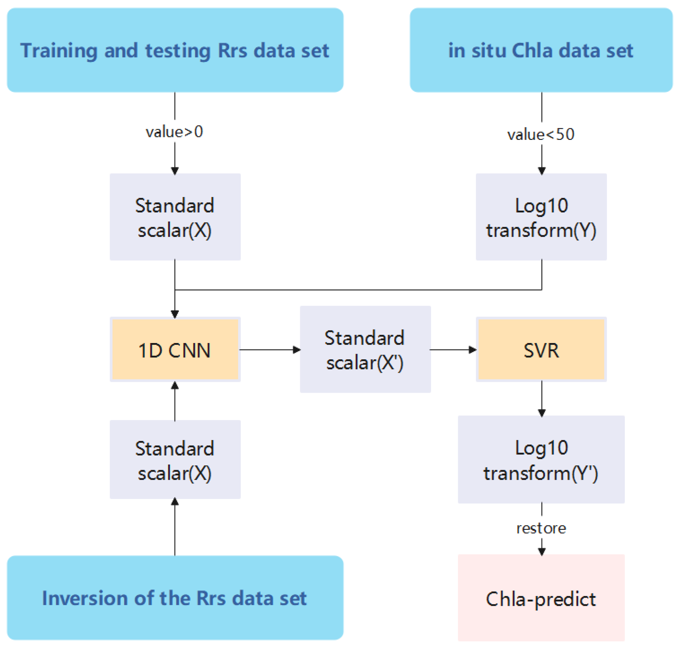
Based on the spectral characteristics of Chla and the complex features of coastal areas, the reflectance data from ten bands (412, 443, 469, 488, 531, 547, 555, 645, 667, and 678) were selected. To reduce noise in the dataset, paired points with Chla concentrations greater than 50 mg/m3 and negative Rrs values were excluded. Through these steps, a more consistent spectral reflectance curve was obtained, and the impact on the true situation was minimized, as shown in Table 1. The reflectance data was then standardized, and the Chla data was transformed using a log10 function. After preprocessing in this manner, both datasets contained no outliers or invalid values and were in approximate ranges, which was beneficial for building the inversion model. The final dataset contained 1271 matched pairs, reduced from the original 1351.

3. Model Development

3.1.1. D CNN/SVR model design

The model used in this paper consists of two algorithms, 1D CNN and SVR, to form a 1D CNN/SVR inversion model. The 1D CNN module is responsible for automatic feature extraction of Rrs, while the SVR module performs regression for fitting Chla concentration. Figure 3 shows the construction process of the inversion model.

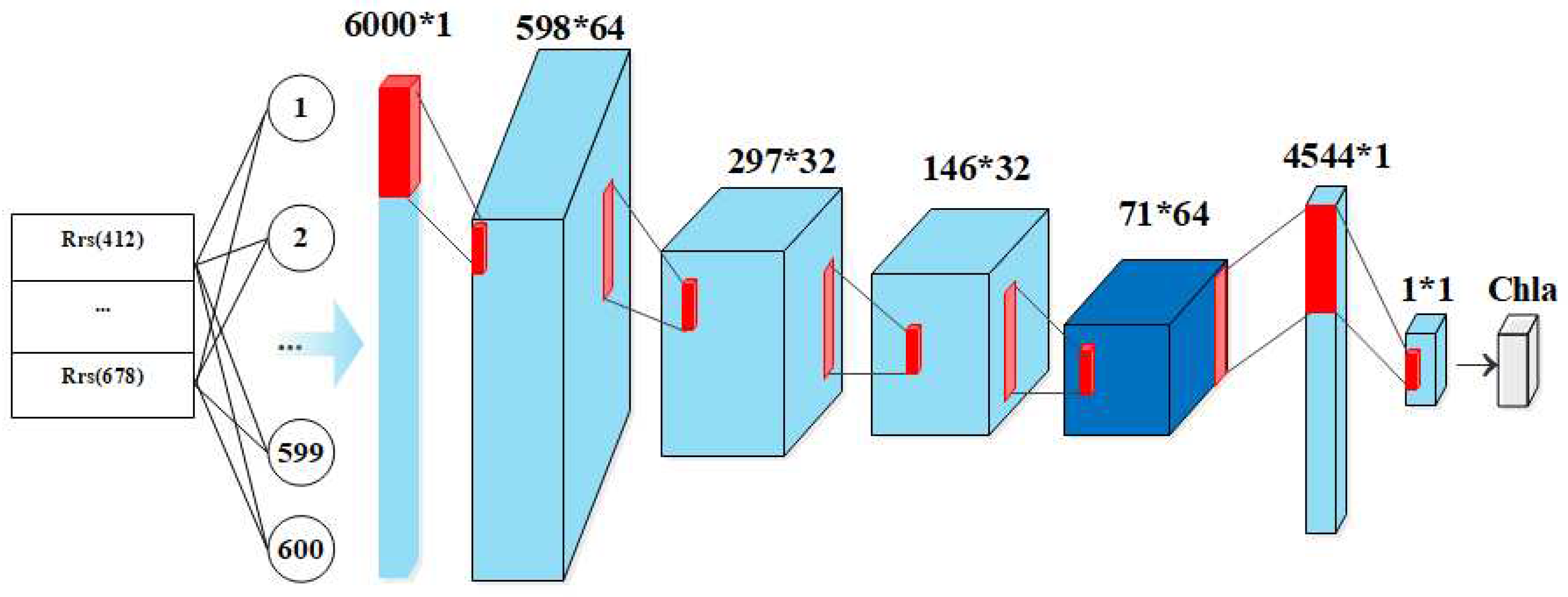
Traditional CNN structures usually consist of multiple convolutional layers, pooling layers, and fully connected layers [25]. The convolutional layers are used for feature extraction, while the pooling layers reduce the size and number of features, thereby reducing the computational complexity of the model. Finally, the fully connected layers transform the features into classification or regression results. However, 1D CNNs differ slightly from traditional CNNs in structure, as the input to the convolutional layer is a three-dimensional vector consisting of samples, time steps, and features, and the output is also a three-dimensional vector consisting of samples, time steps, and channels [26]. In short, 1D CNNs are a type of convolutional neural network designed specifically for processing one-dimensional sequence data. The original dataset used in this paper consisted of two-dimensional vectors, including samples and features, which needed to be converted into three-dimensional vectors. In addition, having too few features may limit the number of convolutional layers that can be used. Therefore, this paper adopted a method of adding features by expanding the feature volume through a fully connected layer. Specifically, we used a fully connected layer with n neuron nodes to perform a full connection operation (F, 1) on the input vector, with an output of (F, n). After the reshape operation, the volume can be restored to its original dimension. However, because 1D CNN is a deep learning model, it may overfit on the training set, while SVR is a non-linear regression model based on kernel functions with good generalization capabilities. Therefore, the final fully connected layer of the 1D CNN was replaced with an SVR module in this paper to achieve regression.

As shown in Figure 4, the 1D CNN/SVR inversion model consists of two modules, a feature extraction module and a regression module. Firstly, a fully connected layer is used to expand the 10 original features (412, 443, 469, 488, 531, 547, 555, 645, 667, and 678) to 600 new input features. The first convolutional layer uses a kernel size of 5, stride of 5, and 64 filters to extract 1200×64 high-dimensional features. Then, three CNN blocks with the same parameters and structure are used to further process the features, each consisting of two convolutional layers and one pooling layer. The kernel size of the convolutional layer is 3, the stride is 1, and there are 32 filters, while the pooling layer uses max pooling with a size of 2. The activation function is uniformly set to the ReLU function. The final regression module is composed of an SVR model, with a regularization parameter of 1 and a kernel function of polynomial kernel and radial basis function, and the other parameters are set to the default values of sklearn.

3.2. Inversion model evaluation metrics

Due to the limitations of standard statistical metrics in Chla inversion algorithms, this paper uses both raw and log-transformed Chla metrics for performance evaluation. The metrics used are as follows:

(1)

(2)

(3)

(4)

(5)

In the Chla concentration prediction process after log10 transformation, R2 is used to evaluate the fitting degree of the regression model, RMSLE is used to measure the difference between the predicted values and the true values, MAE and Bias are used to calculate the mean absolute error between the predicted values and the true values, and the average error of the predicted values, respectively. In addition, the RMSE of the untransformed Chla concentration is also calculated to evaluate the standard deviation.

4. Experiments and Results

4.1. Model performance evaluation

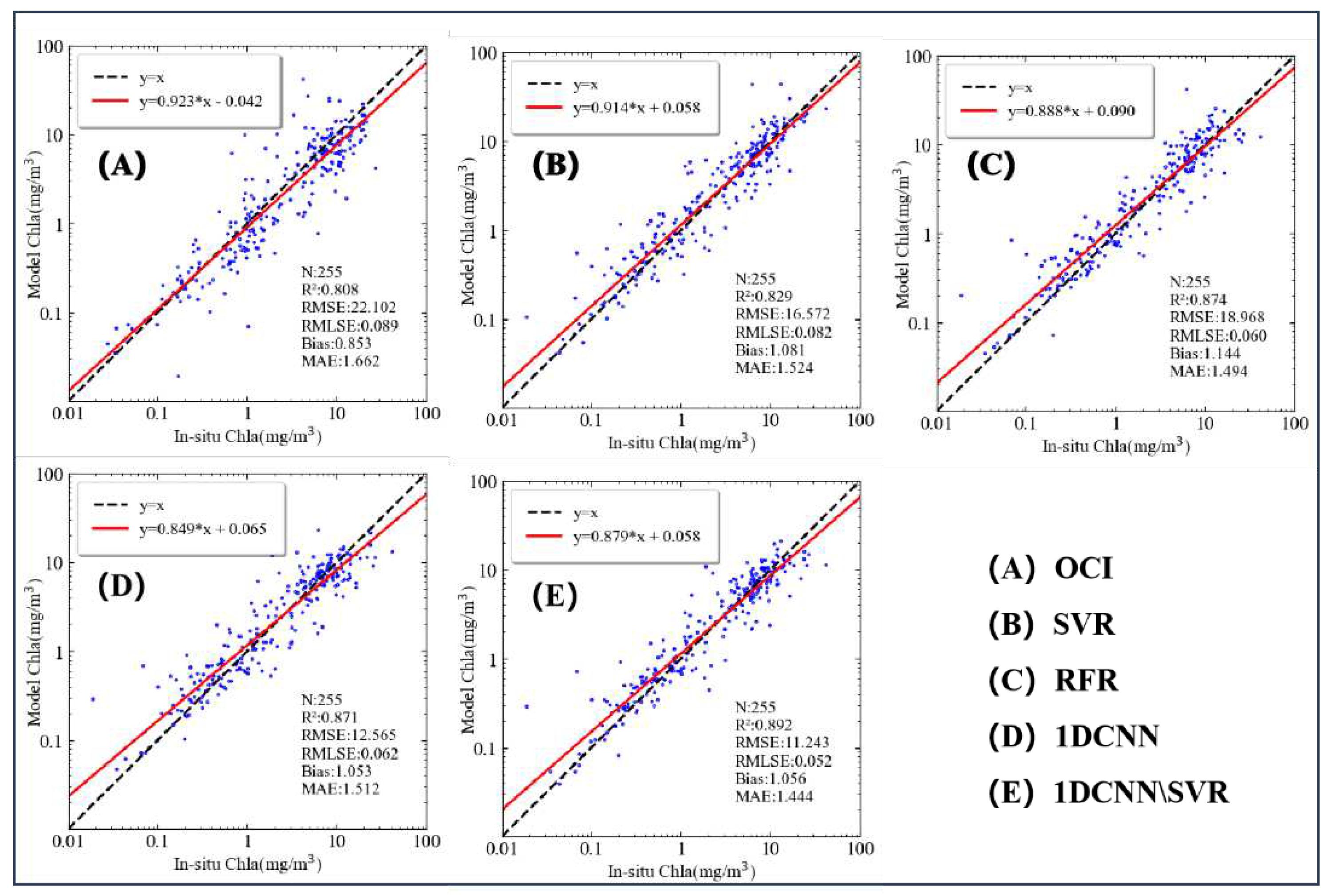
To evaluate the performance metrics of the 1D CNN/SVR inversion model, it was compared with the OCI algorithm, as well as SVR, RFR, and 1D CNN models using the product dataset. To ensure the objectivity of the experiments, the original inputs of all the models were kept consistent, i.e., 10 original features, the same training data (n=1016) and validation data (n=255), and the validation results are shown in Table 2 and Figure 5.

The performance is shown in Figure 6 A-E. The OCI algorithm has poor predictive ability because it is based on an empirical model constructed using global ocean data, while the Chla concentration in coastal waters is influenced by many nonlinear factors, leading to limited prediction accuracy. Among the machine learning algorithms, the SVR algorithm has poor predictive ability, with a total prediction error of 1.081. The predictive ability of the RFR algorithm is better than that of the SVR, with an R² of 0.871 and a reduced prediction error of 1.053. Although the 1D CNN algorithm has better predictive ability than the RFR, the prediction error is as high as 1.144. Finally, the 1D CNN/SVR algorithm has an R² of 0.892, explaining 89.2% of the variance of the target variable. The average error is 11.243 mg/m³, the RMSLE is 0.052, indicating that the prediction error follows a log-normal distribution, the Bias is 1.056, and the MAE is 1.444. These metrics indicate that the model has the strongest predictive ability, the smallest prediction error, and the smallest deviation between the predicted and actual values overall. Therefore, according to the results of this experiment, the 1D CNN/SVR model is the most suitable for Chla concentration inversion in coastal waters.

4.2. Evaluation of the inversion capability of the model at different trophic levels

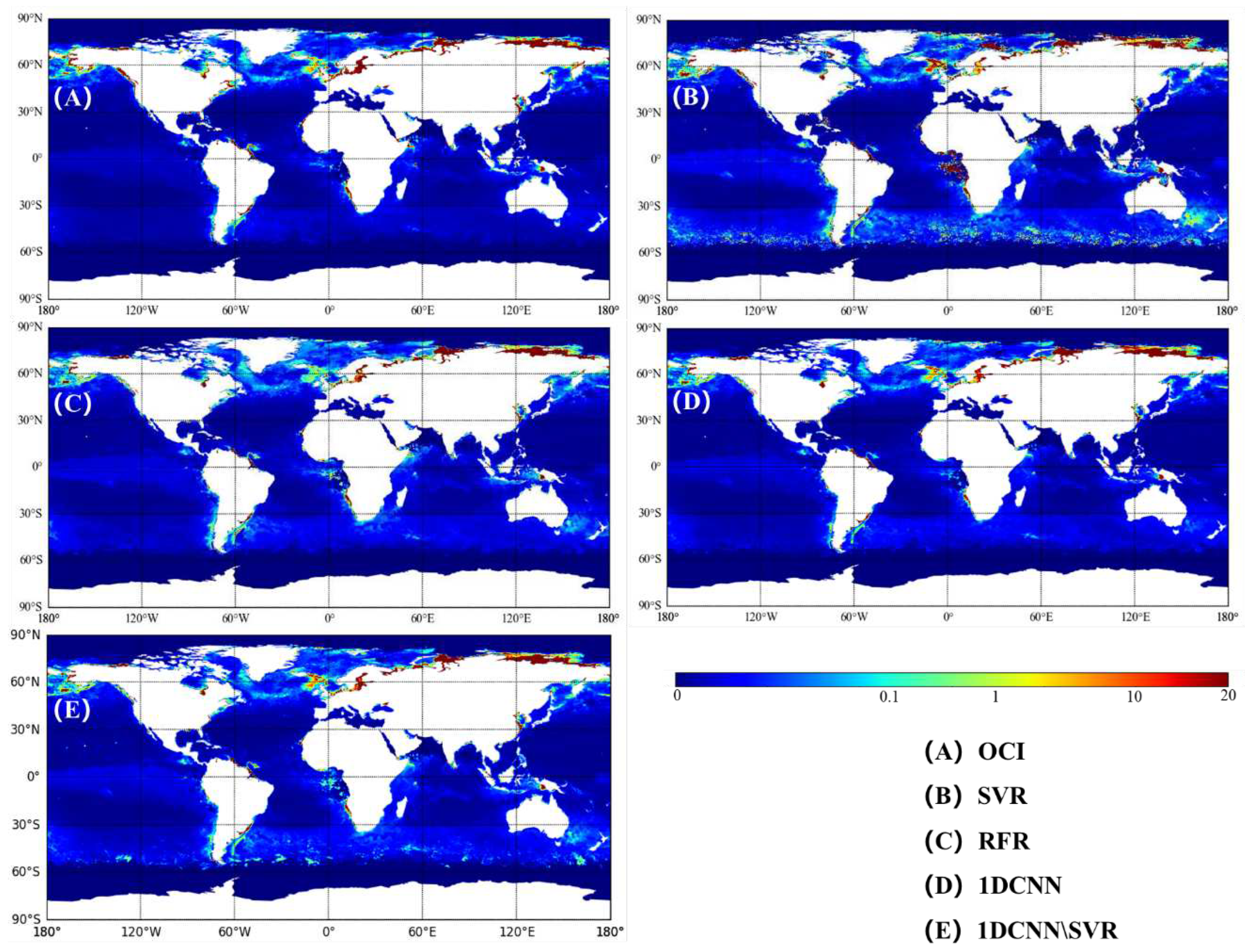
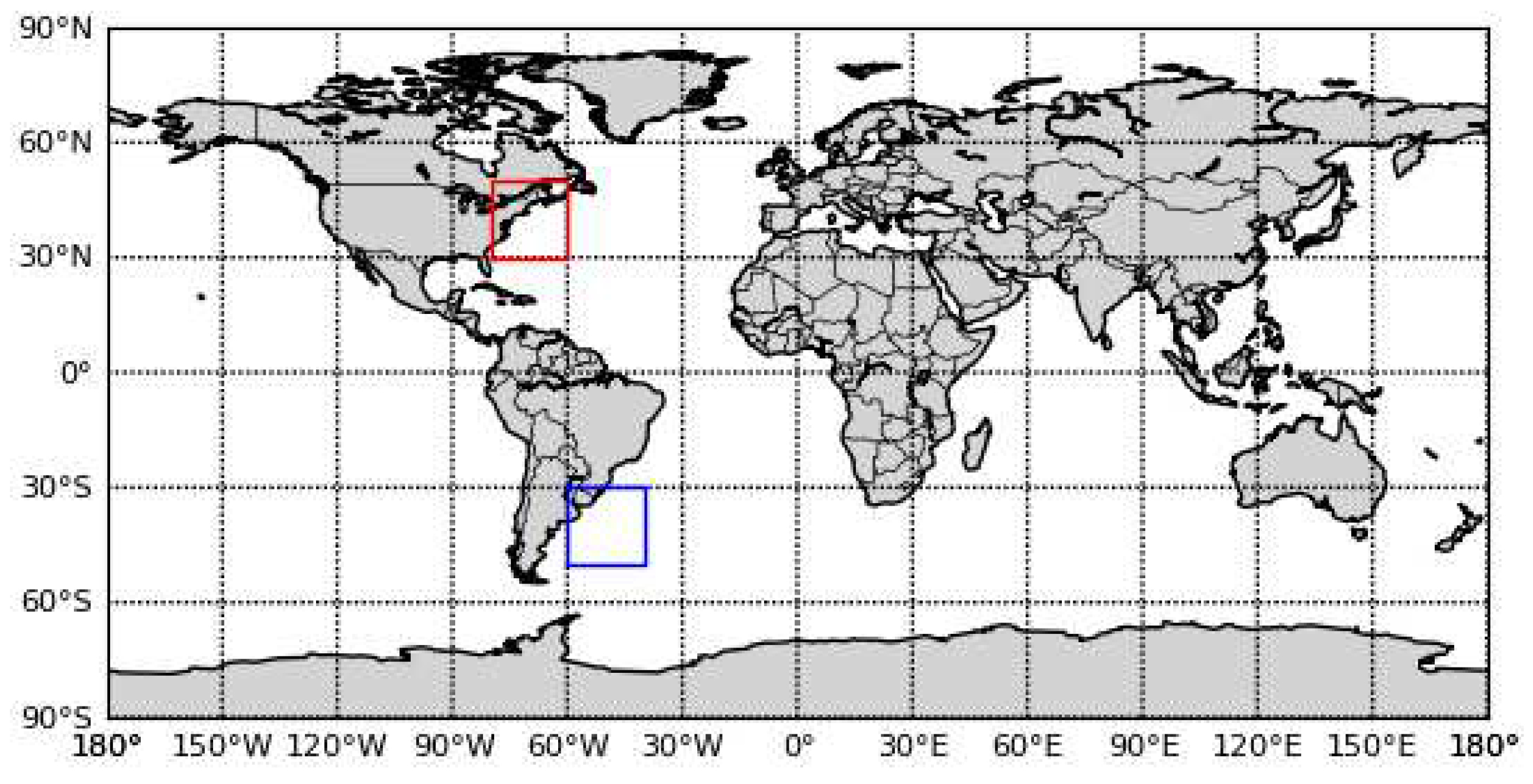
In this section, we evaluated the inversion capability of the model at different trophic levels on a global spatial scale using the monthly average data from August 2003. Figure 7 A-E shows the global spatial distribution of Chla concentration inversion results based on the OCI, SVR, RFR, and 1D CNN/SVR algorithms. The inversion results of these algorithms exhibit similar spatial patterns, such as the characteristics of upwelling near the equator and high Chla concentrations in coastal waters. However, the SVR algorithm shows overestimated Chla concentrations and noise points in the spatial regions of 30°-60°S and 60°-90°N, indicating that the inversion results of this algorithm are sensitive to noise in mid- to high-latitude regions, and the inversion capability is relatively weak. However, the 1D CNN/SVR algorithm did not exhibit this phenomenon, indicating that the 1D CNN used in the first phase of the model can effectively improve this drawback of the SVR algorithm. In addition, there are some differences in performance among the algorithms, as shown in Table 2, but it is difficult to observe the performance differences between the algorithms in the global Chla inversion results, and it is difficult to observe the spatial smoothness of Chla concentrations across different trophic levels, especially in coastal waters. Therefore, we further reduced the spatial scale and selected two regions for inversion, the coastal waters of the North Atlantic (60°-80°W, 30°-50°N) and the southern Indian Ocean (40°-60°E, 30°-50°S), represented as roi_1 (red box) and roi_2 (blue box), respectively, as shown in Figure 7. This is because roi_1 and roi_2 are located in mid- to high-latitude regions, have more in-situ measured points, and have coastal waters with low-nutrient, nutrient-rich, and eutrophic environments [27], which can fully verify the inversion capability of the model in mid- to high-latitude regions with different trophic levels and ensure the accuracy of the inversion results.

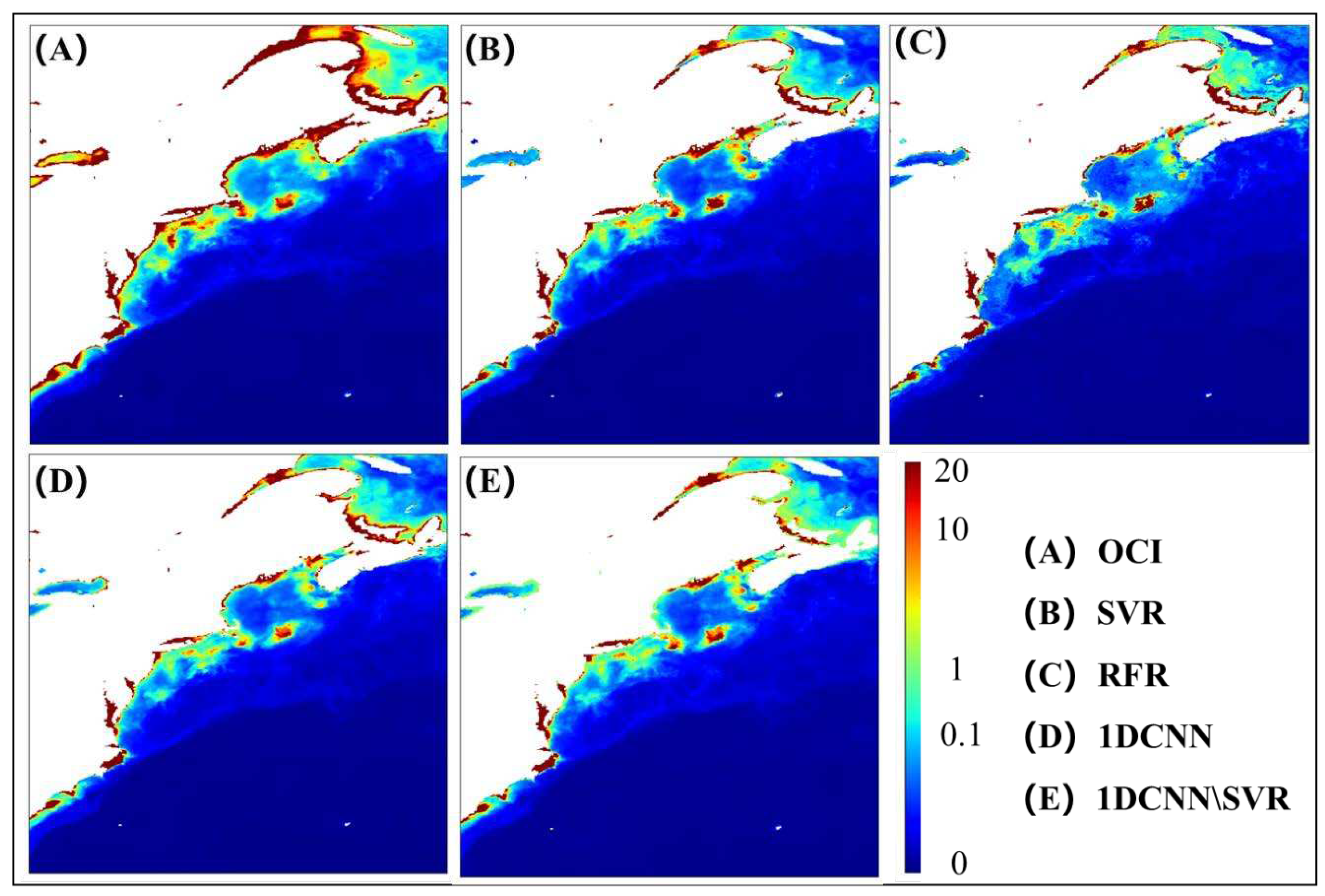
The inversion results of roi_1 are shown in Figure 8A-E. The inversion results of the 1D CNN/SVR model are smoother than those of other algorithms, and there are almost no noise points in the relatively open sea areas. The Chla concentration exhibits a smooth transition in the mesotrophic and eutrophic zones, while the OC3M, SVR, and RFR algorithms show sudden increases. This indicates that other algorithms may be more sensitive to noise, resulting in sudden changes or outliers. In contrast, the 1D CNN/SVR model can better capture and smooth the noise and outliers in the data, thereby improving the accuracy and stability of the inversion results for Chla concentration.

Figure 8 reflects the errors of the four algorithms, OCI, SVR, RFR, and 1D CNN/SVR, in the inversion results of roi_1 compared to the true values, using 100 in-situ data points (N=100). Figure 8A shows that in areas with high Chla concentrations, the OCI algorithm has poor overall fit to the true values, while the SVR and RFR algorithms have improved overall fit but may overestimate Chla concentration. The 1D CNN/SVR algorithm has a higher overall fit and has improved the overestimation of Chla concentration. From Figure 8B and Table 3, it can be seen that the inversion error of RFR is the smallest, but the inversion smoothness of RFR is poor, as shown in Figure 8C. In addition, the average inversion error of the 1D CNN/SVR algorithm is lower than that of SVR but higher than that of 1D CNN, while the maximum and minimum inversion errors are lower than those of 1D CNN. This indicates that 1D CNN/SVR is a combination of SVR and 1D CNN algorithms, complementing each other's disadvantages. However, the accuracy of the model still needs to be improved in practical predictions.

Figure 9. Comparison of inversion errors in roi_1.

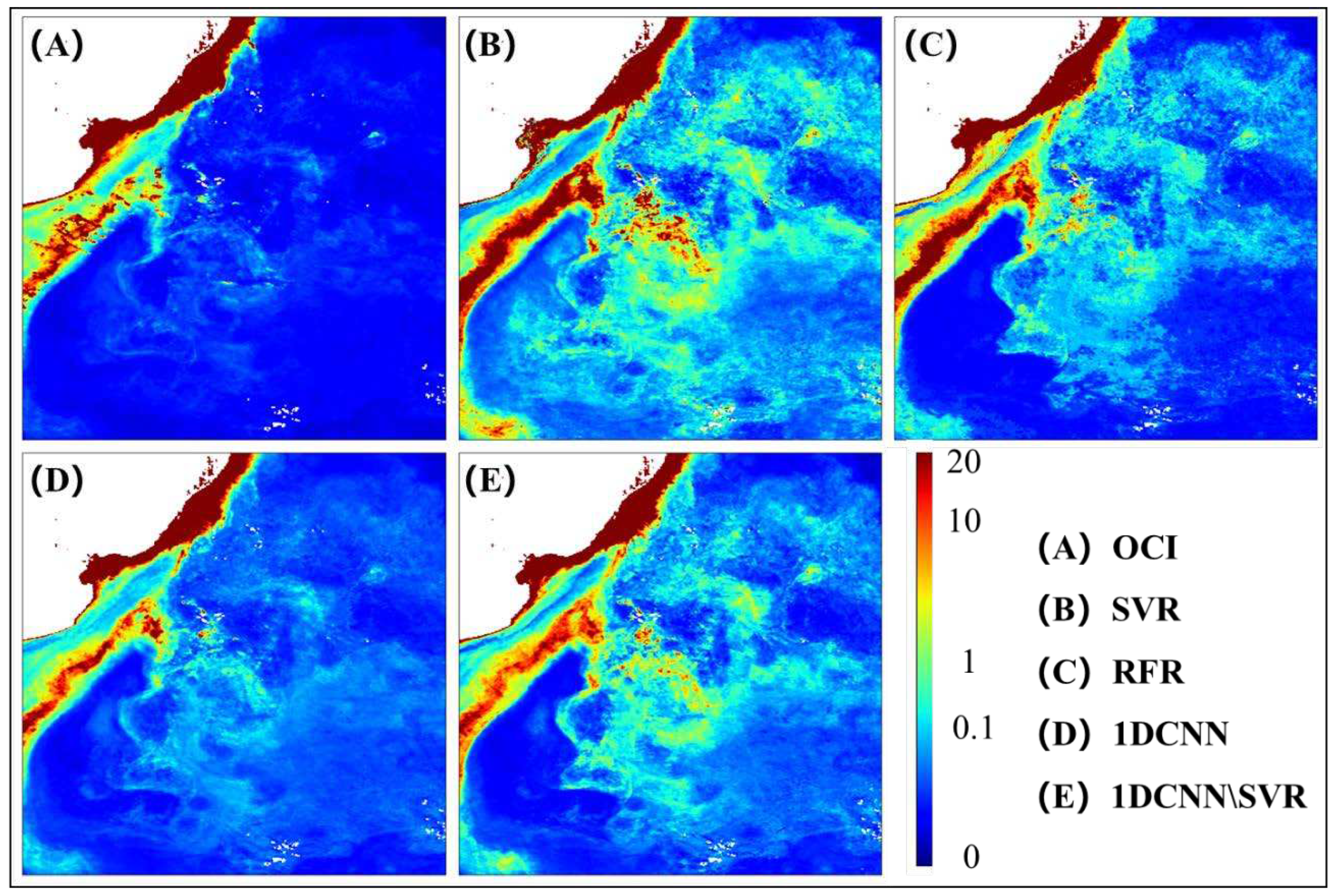
The inversion results of roi_2 are shown in Figure 10A-E. The inversion results of the 1D CNN/SVR model are similar to those of OC3M, indicating that the model has some ability to invert Chla concentration in low-nutrient areas. However, the spatial smoothness of the inversion results is greatly reduced. This is because the training data is mostly concentrated in the nearshore areas, and the 1D CNN/SVR model may pay more attention to the features and patterns of the nearshore areas during the training process, resulting in insufficient feature learning for low-nutrient areas and poor inversion results in these areas.

To further observe the inversion errors of the algorithms, we reduced the number of in-situ data points (N=27) and compared the inversion results of the four algorithms to the true values in roi_2, as shown in Figure 11 and Table 4. It can be observed from Figure 11A that the inversion errors of the algorithms are generally low, but their ability to handle outliers is poor, which is consistent with the inversion results in roi_1. From Figure 11B and Table 4, it can be seen that the minimum and maximum prediction errors of 1D CNN/SVR are lower than those of 1D CNN, confirming that 1D CNN/SVR is a combination of SVR and 1D CNN algorithms.

In summary, compared with other algorithms, the 1D CNN/SVR model can better capture and smooth the noise and outliers in the data, improve the accuracy and stability of the inversion results, and may show more details and fluctuations in the spatial smoothness of the inversion results. However, the ability of the model to invert Chla concentration in low-nutrient areas still needs to be improved.

5. Conclusions

In this study, we developed a global ocean surface chlorophyll-a inversion model based on machine learning. Using ocean chlorophyll-a concentration as the research object, we standardized and removed outliers from the original Rrs before inputting it into the model for prediction. Performance evaluation experiments showed that the 1D CNN/SVR model outperforms current mainstream algorithms, namely OC3M, SVR, RFR, and 1D CNN. Evaluation of inversion capabilities in different nutrient levels showed that the 1D CNN/SVR model addresses the weakness of SVR in inverting chlorophyll-a concentration in middle and high latitudes, and exhibits richer details and higher noise tolerance in the inversion results in nearshore areas, making it a viable alternative for inverting chlorophyll-a concentration in nearshore areas. At the same time, the model also has the ability to invert chlorophyll-a concentration in different nutrient waters, although its performance in low-nutrient areas is slightly weaker, which is a direction for further research.

Author Contributions

For research articles with several authors, a short paragraph specifying their individual contributions must be provided. The following statements should be used “Conceptualization, X.X. and Y.Y.; methodology, X.X.; software, X.X.; validation, X.X., Y.Y. and Z.Z.; formal analysis, X.X.; investigation, X.X.; resources, X.X.; data curation, X.X.; writing—original draft preparation, X.X.; writing—review and editing, X.X.; visualization, X.X.; supervision, X.X.; project administration, X.X.; funding acquisition, Y.Y. All authors have read and agreed to the published version of the manuscript.” Please turn to the CRediT taxonomy for the term explanation. Authorship must be limited to those who have contributed substantially to the work reported.

Funding

Please add: “This research received no external funding” or “This research was funded by NAME OF FUNDER, grant number XXX” and “The APC was funded by XXX”. Check carefully that the details given are accurate and use the standard spelling of funding agency names at https://search.crossref.org/funding. Any errors may affect your future funding.

Data Availability Statement

We encourage all authors of articles published in MDPI journals to share their research data. In this section, please provide details regarding where data supporting reported results can be found, including links to publicly archived datasets analyzed or generated during the study. Where no new data were created, or where data is unavailable due to privacy or ethical restrictions, a statement is still required. Suggested Data Availability Statements are available in section “MDPI Research Data Policies” at https://www.mdpi.com/ethics.

Acknowledgments

In this section, you can acknowledge any support given which is not covered by the author contribution or funding sections. This may include administrative and technical support, or donations in kind (e.g., materials used for experiments).

Conflicts of Interest

Declare conflicts of interest or state “The authors declare no conflict of interest.” Authors must identify and declare any personal circumstances or interest that may be perceived as inappropriately influencing the representation or interpretation of reported research results. Any role of the funders in the design of the study; in the collection, analyses or interpretation of data; in the writing of the manuscript; or in the decision to publish the results must be declared in this section. If there is no role, please state “The funders had no role in the design of the study; in the collection, analyses, or interpretation of data; in the writing of the manuscript; or in the decision to publish the results”.

References

Kasprzak, P. , et al., Chlorophyll a concentration across a trophic gradient of lakes: An estimator of phytoplankton biomass? Limnologica 2008, 38, 327–338. [Google Scholar] [CrossRef]
Amin, S. , et al., Interaction and signalling between a cosmopolitan phytoplankton and associated bacteria. Nature 2015, 522, 98–101. [Google Scholar] [CrossRef] [PubMed]
Ma, J. , et al., Controlling cyanobacterial blooms by managing nutrient ratio and limitation in a large hyper-eutrophic lake: Lake Taihu, China. Journal of Environmental Sciences 2015, 27, 80–86. [Google Scholar] [CrossRef] [PubMed]
Brooks, B.W. , et al., Are harmful algal blooms becoming the greatest inland water quality threat to public health and aquatic ecosystems? Environmental toxicology and chemistry 2016, 35, 6–13. [Google Scholar] [CrossRef]
Lopez, C. , et al., Scientific assessment of freshwater harmful algal blooms. 2008.
Madrid, Y. and Z.P. Zayas, Water sampling: Traditional methods and new approaches in water sampling strategy. TrAC Trends in Analytical Chemistry 2007, 26, 293–299. [Google Scholar] [CrossRef]
O'Reilly, J.E. and PJ. Werdell, Chlorophyll algorithms for ocean color sensors - OC4, OC5 & OC6. Remote Sensing of Environment 2019, 229, 32–47. [Google Scholar]
Hu, C. , A novel ocean color index to detect floating algae in the global oceans. Remote Sensing of Environment 2009, 113, 2118–2129. [Google Scholar] [CrossRef]
Blondeau-Patissier, D. , et al., A review of ocean color remote sensing methods and statistical techniques for the detection, mapping and analysis of phytoplankton blooms in coastal and open oceans. Progress in Oceanography 2014, 123, 123–144. [Google Scholar] [CrossRef]
Tilstone, G.H. , et al., Performance of Ocean Colour Chlorophyll a algorithms for Sentinel-3 OLCI, MODIS-Aqua and Suomi-VIIRS in open-ocean waters of the Atlantic. Remote Sensing of Environment 2021, 260, 112444. [Google Scholar] [CrossRef]
O'Reilly, J.E. and P.J. Werdell, Chlorophyll algorithms for ocean color sensors - OC4, OC5 & OC6. Remote Sensing of Environment 2019, 229, 32–47. [Google Scholar]
Hu, C. L. And and B. Franz, Chlorophyll aalgorithms for oligotrophic oceans: A novel approach based on three-band reflectance difference. Journal of Geophysical Research: Oceans 2012. [Google Scholar] [CrossRef]
Gurlin, D., A. A. Gitelson and W.J. Moses, Remote estimation of chl-a concentration in turbid productive waters — Return to a simple two-band NIR-red model? Remote Sensing of Environment 2011, 115, 3479–3490. [Google Scholar] [CrossRef]
Dall Olmo, G. and A.A. Gitelson, Effect of bio-optical parameter variability on the remote estimation of chlorophyll-a concentration in turbid productive waters: experimental results. Applied Optics 2005, 44, 412–422. [Google Scholar] [CrossRef] [PubMed]
Li, L. , et al., Estimating chlorophyll a concentration in lake water using space-borne hyperspectral data, in Geoscience & Remote Sensing Symposium. 2010.
Liu, F.F. , et al., Retrieval of chlorophyll a concentration from a fluorescence enveloped area using hyperspectral data. International Journal of Remote Sensin 2011, 32, 3611–3623. [Google Scholar] [CrossRef]
Gower, J. , On the use of satellite-measured chlorophyll fluorescence for monitoring coastal waters. International Journal of Remote Sensing 2015, 37, 1–10. [Google Scholar] [CrossRef]
Neil, C.S.E.H. , A global approach for chlorophyll-a retrieval across optically complex inland waters based on optical water types. Remote Sensing of Environment: An Interdisciplinary Journal 2019, 229. [Google Scholar] [CrossRef]
Pahlevan, N. , et al., Seamless retrievals of chlorophyll-a from Sentinel-2 (MSI) and Sentinel-3 (OLCI) in inland and coastal waters: A machine-learning approach. Remote Sensing of Environment 2020, 240, 111604. [Google Scholar] [CrossRef]
Hafeez, S. , et al., Comparison of Machine Learning Algorithms for Retrieval of Water Quality Indicators in Case-II Waters: A Case Study of Hong Kong. Remote Sensing 2019, 11, 617. [Google Scholar] [CrossRef]
Le, C. , et al., Evaluation of chlorophyll-a remote sensing algorithms for an optically complex estuary. Remote Sensing of Environment 2013, 129, 75–89. [Google Scholar] [CrossRef]
Sadaiappan, B. , et al., Applications of Machine Learning in Chemical and Biological Oceanography. ACS Omega 2023, 8, 15831–15853. [Google Scholar] [CrossRef]
Zhao, X. , et al., Comparing deep learning with several typical methods in prediction of assessing chlorophyll-a by remote sensing: a case study in Taihu Lake, China. 2021.
Yu, B. , et al., Global chlorophyll-a concentration estimation from moderate resolution imaging spectroradiometer using convolutional neural networks. Journal of Applied Remote Sensing 2020, 14. [Google Scholar]
Li, Z. , et al., A Survey of Convolutional Neural Networks: Analysis, Applications, and Prospects. IEEE Transactions on Neural Networks and Learning Systems 2021. [Google Scholar]
Tang, W. , et al., Rethinking 1D-CNN for Time Series Classification: A Stronger Baseline. 2020.
Seegers, B.N. , et al., Performance metrics for the assessment of satellite data products: an ocean color case study. Optics Express 2018, 26, 7404–7422. [Google Scholar] [CrossRef] [PubMed]

Figure 1. Shows the spatiotemporal distribution of MODIS-Aqua matched with true values.

Figure 2. Shows the spatial distribution of the training set (left) and validation set (right) point locations.

Figure 3. Shows the spatial distribution of the training set (left) and validation set (right) point locations.

Figure 4. Shows the structure of the 1D CNN/SVR inversion model.

Figure 5. Validation set prediction results.

Figure 6. Global Chla concentration inversion (August 2003).

Figure 7. Local inversion regions (roi_1 and roi_2).

Figure 8. Inversion results of roi_1 (60°-80°W, 30°-50°N).

Figure 10. Inversion results of roi_2 (40°-60°E, 30°-50°S).

Figure 11. Comparison of inversion errors in roi_2.

Table 1. Statistical results before and after data preprocessing.

Data type	Before preprocessing			After preprocessing
Data type	Min	Max	Mean	Min	Max	Mean
Rrs_412(sr-1)	-0.00354	0.01914	0.00336	0.00001	0.01914	0.00355
Rrs_443(sr-1)	-0.00201	0.02393	0.00327	0.00009	0.02393	0.00344
Rrs_469(sr-1)	-0.00129	0.02973	0.00373	0.00055	0.02973	0.00388
Rrs_488(sr-1)	-0.00073	0.03174	0.00378	0.00049	0.03174	0.00392
Rrs_531(sr-1)	0.000883	0.02765	0.00415	0.00088	0.02765	0.00425
Rrs_547(sr-1)	0.000846	0.02539	0.00418	0.00102	0.02539	0.00427
Rrs_555(sr-1)	0.000795	0.02306	0.00403	0.00102	0.02306	0.00410
Rrs_645(sr-1)	-0.00047	0.01438	0.00156	0.00001	0.01438	0.00159
Rrs_667(sr-1)	-0.00041	0.01277	0.00127	0.00001	0.01277	0.00130
Rrs_678(sr-1)	-0.00032	0.01226	0.00130	0.00002	0.01226	0.00133
Chl-a(mg/m³)	0.019	58.099	4.945	0.019	46.350	4.708

Table 2. Numerical values of evaluation metrics on the validation.

Algorithm	R²	Slope	RMSE(mg/m³)	RMLSE	Bias	MAE
OCI	0.808	0.923	22.102	0.089	0.853	1.662
SVR	0.829	0.914	16.572	0.082	1.081	1.524
RFR	0.871	0.849	12.565	0.062	1.053	1.512
1DCNN	0.874	0.888	18.968	0.060	1.144	1.494
1DCNN/SVR	0.892	0.879	11.243	0.052	1.056	1.444

Table 3. Minimum, Maximum, and Average Inversion Errors(roi_1).

	OCI	SVR	RFR	1DCNN	1DCNN\SVR
Min	-12.804	-5.747	-5.092	-5.429	-4.651
Max	14.619	6.810	5.968	12.940	12.669
Average	-1.416	-0.296	-0.130	-0.154	-0.190

Table 4. Minimum, Maximum, and Average Inversion Errors(roi_2).

	OCI	SVR	RFR	1DCNN	1DCNN\SVR
Min	-11.695	-2.096	-4.446	-3.254	-2.667
Max	11.156	4.553	1.5071	8.611	8.173
Average	-1.007	-0.219	-0.009	-0.254	-0.268

Disclaimer/Publisher’s Note: The statements, opinions and data contained in all publications are solely those of the individual author(s) and contributor(s) and not of MDPI and/or the editor(s). MDPI and/or the editor(s) disclaim responsibility for any injury to people or property resulting from any ideas, methods, instructions or products referred to in the content.

© 2023 by the authors. Licensee MDPI, Basel, Switzerland. This article is an open access article distributed under the terms and conditions of the Creative Commons Attribution (CC BY) license (http://creativecommons.org/licenses/by/4.0/).

Copyright: This open access article is published under a Creative Commons CC BY 4.0 license, which permit the free download, distribution, and reuse, provided that the author and preprint are cited in any reuse.

MDPI Initiatives

Important Links

Choose an area of interest and we will send you notifications of new preprints at your preferred frequency.

Disclaimer