Theoretical Validation and Hardware Implementation of Dynamic Adaptive Scheduling for Heterogeneous Systems-on-Chip

Domain-specific systems-on-chip (DSSoCs) aim to narrow the gap between general-purpose processors and application-specific designs. CPU clusters enable programmability, while hardware accelerators tailored to the target domain minimize task execution times and power consumption. Traditional operating system (OS) schedulers can diminish the potential of DSSoCs as their execution times can be orders of magnitude larger than the task execution time. To address this problem, we propose a dynamic adaptive scheduling (DAS) framework that combines the advantages of a fast, low-overhead scheduler and a sophisticated, high-performance scheduler with a larger overhead. We present a novel runtime classifier that chooses the better scheduler type as a function of the system workload, leading to improved system performance and energy-delay product (EDP). Experiments with five real-world streaming applications indicate that DAS consistently outperforms fast, low-overhead, and slow, sophisticated schedulers. DAS achieves a 1.29x speedup and 45% lower EDP than the sophisticated scheduler under low data rates and a 1.28x speedup and 37% lower EDP than the fast scheduler when the workload complexity increases. Furthermore, we demonstrate that the superior performance of the DAS framework also applies to hardware platforms, with up to a 48% and 52% reduction in execution time and EDP, respectively.

Keywords:

domain-specific SoC (DSSoC)

;

task scheduling

;

runtime classification

;

policy switching

Subject:

Computer Science and Mathematics - Hardware and Architecture

1. Introduction

Heterogeneous systems-on-chip (SoCs) combine the energy efficiency and performance of custom designs with the flexibility benefits of general-purpose cores. Domain-specific SoCs (DSSoCs), a subset of heterogeneous SoCs, are emerging examples that integrate general-purpose compute elements and hardware accelerators that target the commonly encountered tasks (i.e., computational kernels) in the target domain [2,3,4,5]. For example, a DSSoC for autonomous driving incorporates computer vision and deep learning accelerators, while a DSSoC for 5G/6G communication domain accelerates signal processing operations, such as fast Fourier transform (FFT). In addition, general-purpose CPU clusters and programmable accelerators, such as coarse-grained reconfigurable architectures (CGRA), offer alternative execution paths for a broader set of tasks, besides improving flexibility [3,6].

In contrast to fixed-function designs, a critical distinction of DSSoCs is their ability to run multiple applications from the same domain [7]. When multiple applications run concurrently, the number of ready tasks can exceed the capacity of the available accelerators resulting in resource contention. This resource contention leads to a complex runtime scheduling problem since there are many different ways to prioritize and run such tasks. For example, waiting for the most suitable resource to become available can lead to higher energy efficiency than resorting to an immediately available less suitable resource like a CPU core or a reconfigurable accelerator. Besides the complex runtime scheduling problem, recent studies show that execution times for applications of domain-specific systems are on the nanosecond scale [2,8]. Therefore, the classical scheduling problem encounters a new challenge in heterogeneous DSSoCs because domain-specific tasks can run in the order of nanoseconds, i.e., at least two or three orders of magnitude faster than general-purpose cores when they are executed on their specialized pipelines. If the scheduler takes a significantly longer amount of time to make a decision, it can undermine the benefits of hardware acceleration. For instance, Linux Completely Fair Scheduler (CFS) takes

1.2 μ s

to make a scheduling decision when running on an Arm Cortex-A53 core [9,10,11,12]. This overhead is clearly unacceptable when there are many tasks with orders of magnitude faster execution times.

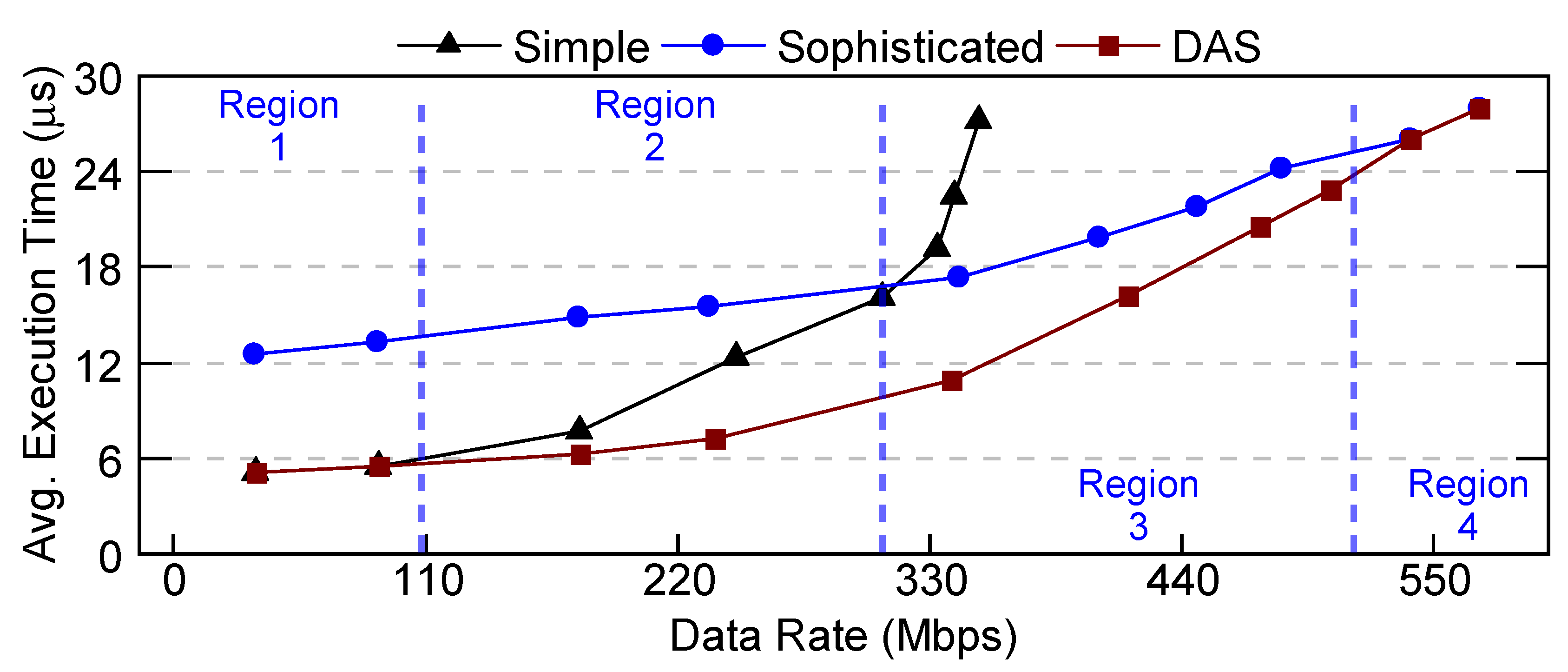
DSSoCs require fast scheduling algorithms to keep up with tasks that can run in the order of nanoseconds and achieve high efficiency. However, poor scheduling decisions of simple low-overhead schedulers can decrease the system performance, especially under heavy workloads. For example, Figure 1 shows the average execution time and energy-delay product for a workload mix of a wireless communication system. When the data rate is low (i.e., few frames are present concurrently), there is lower contention for the same SoC resources. Hence, a fast low-overhead scheduler (in this work, a lookup table) outperforms a more sophisticated scheduler (e.g., a complex heuristic or an integer programming-based scheduler) since it can make the same or very similar assignments with a significantly lower overhead. As the data rate increases, the number of concurrent frames, and hence the complexity of scheduling decisions, also grow. At the same time, the waiting times of the tasks in the core queues exceed their actual execution time in the accelerators. Therefore, a sophisticated scheduler outperforms the simple one (point A in Figure 1a), and the overhead of making better scheduling decisions pays off. In contrast, when an application involves a high degree of task-level parallelism, we expect more tasks in the ready queue waiting for a scheduling decision. For such applications, the scheduling overhead can dominate the execution time, even for lower data rates (Figure 1b). For these cases, using a sophisticated scheduler cannot outperform the scheduling decisions of a simple scheduler. As the data rate increases, a sophisticated scheduler can degrade the system performance because of its dependence on the number of ready tasks. Therefore, a simple scheduler outperforms a sophisticated scheduler under various data rates. Hence, the trade-off between the scheduling decision quality and the scheduling overhead is an opportunity to exploit.

To exploit the trade-off between the scheduler overhead and decision quality, we propose a dynamic adaptive scheduling (DAS) framework that combines the benefits of the sophisticated and simple low-overhead scheduling algorithms using an integrated support mechanism. Making a scheduling decision at the scale of nanoseconds is highly challenging because executing possibly complex decisions and loading the necessary context, such as performance counters, requires extra time. Hence, even the data movement part alone can violate the fast decision target. Moreover, the framework needs to determine at runtime whether the low-overhead or sophisticated scheduler should run. The DAS framework outperforms both underlying schedulers despite these challenges by following these key observations in the design process: First,, the scheduling will be called with 100% certainty and uses features (a subset of available performance counters). Therefore, prefetching the required features in a background process and writing them to a pre-allocated local memory location can hide the extra overhead. Second, the choice of a sophisticated or a simple scheduler can be made by the same prefetching process before the following scheduling process begins. If the simple scheduler is chosen, the only extra overhead on the critical path is the time to access the LUT, which is measured as 6 ns on Arm Cortex-A53. We run the sophisticated scheduler at runtime only if a more complex scheduler is needed.

A preliminary version of this work appeared in the IEEE Embedded Systems Letters [1], where we presented the concept of dynamic adaptive scheduling using high-level event-driven simulations. It showed that adaptively using a slow and fast scheduler can enable better performance and energy efficiency than any of the schedulers alone. However, the preliminary work relied on high-level simulations without theoretical ground and experimental evaluation. This paper expands the preliminary work significantly and makes the following novel contributions:

Theoretical proof of DAS framework and its experimental validation using a DSSoC simulator [13];
Integration of the DAS framework with an open-source runtime environment [6] and its training and deployment on Xilinx Zynq ZCU102 SoC [14];
Extensive performance evaluation in the trade space of execution time, energy, and scheduling overhead over the Xilinx Zynq ZCU102 SoC based on workload scenarios composed of real-life applications;

The rest of the paper is organized as follows. Section 2 reviews the related work. We describe the proposed DAS framework and algorithms in Section 3. Section 4 discusses and analyzes the experimental results on a DSSoC simulator with real-world applications, while Section 5 presents the training and implementation details of the DAS framework on an FPGA emulation environment using real-world applications. Finally, Section 6 concludes the paper.

2. Related Work

Schedulers have evolved significantly to adapt to different requirements and optimization objectives. Static [15,16] and dynamic [11,17,18,19] task scheduling algorithms have been proposed in the literature. Completely Fair Scheduler (CFS) [11] is a dynamic approach that is widely used in Linux-based OS and aims to provide resource fairness to all processes while the static approaches presented in [15,16] optimize the makespan of applications. CFS [11] was initially developed for homogeneous platforms, but it can also handle heterogeneous architectures (e.g., Arm big.LITTLE). While CFS may be effective for client and small-server systems, high-performance computing (HPC) and high-throughput computing (HTC) necessitate different scheduling policies. These policies, such as Slurm and HTCondor, are specifically designed to manage a large number of parallel jobs and meet high-throughput requirements [20,21]. On the other hand, DSSoCs demand a novel suite of efficient schedulers that execute at nanosecond-scale overheads since they deal with scheduling tasks that can execute in the order of nanoseconds.

The scheduling overhead problem and scheduler complexities are discussed in [22,23,24,25,26,27,28]. The authors in [22] propose two dynamic schedulers, named as CATS and CPATH, where CATS detect the longest and CPATH detects the critical paths in the application. CPATH algorithm shows inefficiency in terms of its higher scheduling overhead. Motivated by high scheduling overheads, [10] propose a new scheduler that approximates an expensive heuristic algorithm using imitation learning with low overhead. An imitation learning-based scheduler approximates an expensive heuristic with a low overhead [10]. However, the scheduling overhead is still approximately

1.1 μ s

, making it inapplicable for DSSoCs with nanosecond-scale task execution. Energy-aware schedulers for heterogeneous SoCs have limited applicability to DSSoCs because of their complexity and large overheads [29,30,31,32].

Several scheduling algorithms that demonstrate the benefits of using multiple schedulers are proposed in [33,34,35]. Specifically, the authors in [33] propose a technique that switches between three schedulers dynamically to adapt to varying job characteristics. However, the overheads of switching between policies are not considered as part of the scheduling overhead. The approach in [35] integrates static and dynamic schedulers to exploit both design-time and runtime characteristics for homogeneous processors. The hybrid scheduler in [35] uses a heuristic list-based schedule as a starting point and then improves it using genetic algorithms. However, it does not consider the scheduling overhead of the individual schedulers. The authors in [23] discuss the performance comparison of a simple round-robin scheduler and a complex earliest deadline first (EDF) scheduler and their applicability under different system load scenarios.

Using insights from literature, we propose a novel scheduler that combines the benefits of the low scheduling overhead of a simple scheduler and the decision quality of a sophisticated scheduler (described in Section 3.3) based on the system workload intensity. To the best of our knowledge, this is the first approach that uses a novel runtime preselection classifier to choose between simple and sophisticated schedulers at runtime to enable scheduling with low energy and nanosecond scale overheads in DSSoCs.

3. Dynamic Adaptive Scheduling Framework

In this section, we start with introducing the preliminaries used in the proposed DAS approach (Section 3.1) and then present the dataset generation process and the online usage of DAS models (Section 3.2). Finally, we present the selection of fast and sophisticated schedulers in Section 3.3.

3.1. Overview and Preliminaries

This work considers streaming applications that can be modeled by data flow graphs (DFGs). More precisely, consecutive data frames are pipelined through the tasks in the graph. The current practice of scheduling is limited to a single scheduler policy. On the other hand, DAS allows the OS to choose one scheduling policy

π \in Π_{S} = {F, S}

, where F and S refer to the fast and slow (or sophisticated) schedulers, respectively. When the task becomes ready (predecessors of the task are completed), the OS can call either a slow (

π = S

) or a fast (

π = F

) scheduler as a function of the workload and system state. The OS collects a set of performance counters during the execution to enable two aspects for the DAS framework: (1) precise assessment of the system state, (2) desirable features for the classifier to switch between the fast and slow schedulers at runtime. Table 1 shows the various types of performance counters that are collected for the DAS framework. The total number of performance counters is 62 for a DSSoC with 19 PEs. The goal of the slow scheduler S is to handle more complex scenarios when the task wait times dominate the execution times. In contrast, the fast scheduler F aims to approach the theoretically minimum (i.e., zero) scheduling overhead by making decisions in a few cycles with a minimum number of operations. The DAS framework aims to outperform both underlying schedulers by dynamically switching between them as a function of system state and workload.

3.2. DAS Preselection Classifier

The first runtime decision of DAS is the selection of the fast or slow scheduler. We should optimize this decision to approach the goal of zero scheduling overhead as it is on the critical path of both schedulers. One of the novel contributions of DAS is that we recognize this selection as a deterministic task that will be eventually executed with a probability of one. Therefore, we prefetch the relevant features that are required for this decision to a pre-allocated local memory. We re-use a subset of the performance counters which are shown in Table 1 as desirable features to minimize the scheduling overhead. The relevant subset of features is presented in Section 4.2. To reflect the system state at that point in time, the OS periodically refreshes the performance counters. DAS framework runs a light-weight classifier which determines whether the fast or slow scheduler should be used for the next ready task each time the features are refreshed. As it is refreshed with the features that reflect the most recent system state, we note that this decision will always be up to date. Thus, DAS can determine which scheduler should be called even before a task is ready for scheduling. Consequently, the preselection classifier of DAS framework introduces zero latency and minimal energy overhead, as described next.

Offline Classifier Design: The first step for the design process of the preselection classifier is to generate the training data based on the domain applications known at design time. Each scenario in the training data consists of concurrent applications and their respective data rates. For example, a combination of WiFi transmitter and receiver chains, at a specific upload and download speed, could be one such scenario. To this end, we run each scenario twice on an instrumented hardware platform or a simulator (see Figure 2).

First Execution: The instrumentation enables us to run both fast and slow schedulers each time a task scheduling decision is made. We note that the scheduler is invoked whenever a task is to be scheduled. If the decisions of the fast (

D_{F}

) and slow (

D_{S}

) schedulers for a task

T_{i}

are identical, then we label task

T_{i}

with F (i.e., the fast scheduler) and store a snapshot of the performance counters. The label F implies that the fast scheduler can reach the same scheduling decision as the sophisticated algorithm under the system states captured by the performance counters. If the decisions of the schedulers are different, then the label is left as pending and the execution continues by following the decision of the fast scheduler, as described in Figure 2. At the end of the execution, the training data contains a mix of both labeled (F) and pending decisions.

Second Execution: The same scenario is executed for the second time. This time the execution always follows the decisions of the slow scheduler. At the end of the execution, we analyze the target metric, such as the average execution time or the total energy consumption. If a better result can be achieved by using the slow scheduler, the pending labels are replaced with S to indicate that the slow scheduler is preferred despite its larger overhead. Otherwise, we conclude that the lower overhead of the fast scheduler pays off, and the pending labels are replaced with F. An alternative approach is to evaluate each pending instance individually; however, this would not offer a scalable solution as scheduling is a sequential decision-making problem, and a decision at time

t_{k}

affects the remaining execution.

In this work, the training data is generated using 40 distinct workloads. Each workload is a mix of multiple instances of five applications, consisting of approximately 140,000 tasks in total and executed at 14 different data rates, as detailed in Section 4.1 and Appendix B. A higher data rate presents a larger number of concurrent applications contending for the same SoC resources. Then, we design a low-overhead classifier using machine learning techniques and feature selection methods [36], as described in Section 4.2.

Online Use of the Classifier: At runtime, a background process periodically updates a pre-allocated local memory with the subset of performance counters that the classifier requires for the scheduler selection. After each update, the classifier determines whether the fast F or slow S scheduler should be used for the next available task. When a new ready task becomes available, the features are already loaded and we know which scheduler is a better choice for the read task. Therefore, DAS framework does not incur any extra delay on the critical path. Moreover, it has a negligible energy overhead, as demonstrated in Section 4, which is critical for the performance and applicability of such an algorithm.

3.3. Fast & Slow (F&S) Scheduler Selection

The proposed DAS framework can work with any choice of fast and slow scheduling algorithms. This work uses a lookup table (LUT) implementation as the fast scheduler as the goal of the fast scheduler is to achieve almost zero overhead. The LUT stores the most energy-efficient processor in the target system as a decision for each known task in the target domain. Unknown tasks are mapped to the next available CPU core. Hence, the LUT access at runtime is the only extra delay on the critical path and overhead of the fast scheduler. To profile the scheduling overhead of LUT, we developed an optimized C implementation with inline assembly code. Experiments show that our fast scheduler takes ∼7.2 cycles (6 ns on Arm Cortex-A53 at 1.2 GHz) on average, and incurs negligible (2.3 nJ) energy overhead.

The DAS framework uses a commonly used heuristic, earliest task first (ETF) as the slow scheduler [37]. ETF is chosen since it recursively iterates over the ready queue tasks and processors to provide the schedule that achieves the fastest finish time, as shown in Algorithm 1. It performs a comprehensive search which can make the best decision when the system is loaded with many tasks. Hence, its computational complexity is quadratic with respect to the number of ready tasks. The detailed computational and energy overhead of ETF are presented in Section 4.1.

Algorithm 1 ETF Scheduler

1:: while ready queue $T$ is not empty do
2:: for task $T_{i}$ $\in T$ do
3:: /* $P$ = set of PEs */
4:: for PE $p_{j}$ $\in P$ do
5:: $F T_{T_{i}, p_{j}}$ = Compute the finish time of $T_{i}$ on $p_{j}$
6:: end for
7:: end for
8:: ( $T^{'}$ , $p^{'}$ ) = Find the task and PE pair that has the minimum FT
9:: Assign task $T^{'}$ to PE $p^{'}$
10:: end while

The detailed theoretical proof that shows DAS achieves superior performance over the baseline schedulers and its experimental validation are presented in Appendix A.

4. Evaluation of DAS Using Simulations

Section 4.1 describes the experimental setup used in this work. Section 4.2 explores different machine learning methods and features for DAS. The evaluation and detailed analysis of DAS for different workloads is shown in Section 4.3. Finally, we demonstrate the latency and energy consumption overheads of DAS in Section 4.4.

4.1. Simulation Setup

This section presents the setup used for profiling scheduling overhead of complex and basic schedulers, simulation framework that has been used for performance analysis and training data generation, and SoC configuration that we used.

Domain Applications: The DAS framework is evaluated using five real-world streaming applications: range detection, temporal mitigation, WiFi-transmitter, WiFi-receiver applications and a proprietary industrial application (App-1), as summarized in Table 2. We then construct 40 different workloads for runtime analysis of the schedulers used in this paper. All workloads are run in streaming mode, and for each data point in the figures in Section 4.3, approximately 10,000 tasks are scheduled. Details of the workload mixes are given in Appendix B.

Emulation Environment: Conducting a realistic runtime overhead and energy analysis is one of our key goals in this study. For this purpose, we leverage a Compiler-integrated, Extensible DSSoC Runtime (CEDR) framework introduced by Mack et al. [6]. The CEDR has been validated extensively on x86 and Arm-based platforms. It enables pre-silicon performance evaluations of heterogeneous hardware configurations composed of mixtures of CPU cores and accelerators based on dynamically arriving workload scenarios. Compared to the other emulation frameworks (e.g., ZeBu [38] and Veloce [39]), this portable and open-source environment offers distinct plug-and-play integration points where developers can individually integrate and evaluate their applications, scheduling heuristics, and accelerator IPs in a realistic system.

The emulation framework [40] combines compile-time analysis with the run-time system. The compilation process involves converting each application to LLVM intermediate representation (IR), identifying what section of the code should be labeled as “kernels” (frequently executing IR-level blocks) or “non-kernels”, and automatically refactoring the LLVM IR into a directed acyclic graph (DAG), where each node represents a kernel. By abstracting the application with a DAG, compile-time flow generates a flexible binary structure for the run-time system to be able to invoke each function call on all its supported processing elements (PEs) in the target architecture. The runtime system monitors the state of system resources, parses dynamically the arriving applications, generates the queue of tasks that have resolved dependencies (called ready queue), schedules the ready queue tasks based on the user-defined scheduling policy and manages the data transfers to and from the PEs. The run-time system supports scheduling heuristics, such as Round Robin, Earliest Finish Time (EFT), and Earliest Task First (ETF). We selected ETF scheduler as the complex scheduler of our analysis because of its complexity and quality decisions that it provides. As shown in Algorithm 1, ETF recursively iterates over the ready queue tasks and PEs with the objective of finding the task to PE mapping decisions that result with the minimum finish time. It does this process recursively until each ready task is scheduled to a PE.

We generate a wide range of workloads – ranging from all application instances belonging to a single application to a uniform distribution from all five applications to evaluate the impact of the scheduling overhead of ETF. We present the impact of the number of tasks in the ready queue on the scheduling overhead of ETF in Figure 3, as measured on the Xilinx Zynq ZCU102. The x-axis in the plot shows the number of tasks that are in the ready queue for each workload scenario, and the y-axis shows the scheduling overhead of the ETF scheduler. We generate a quadratic equation to formulate the ETF scheduling overhead observed at runtime based on these measurements. Later, we utilize this equation to evaluate the average execution time and the EDP of the DAS scheduler on the simulator. We note that the DAS framework is by no means limited to the processors, schedulers, and applications that are used for demonstration purposes.

Simulation Environment: We use DS3 [13], an open-source domain-specific system-on-chip simulation framework, to perform detailed evaluations of our proposed scheduling approach. DS3 is a high-level simulation tool that includes built-in scheduling algorithms, models for PEs, interconnect, and memory systems. The framework has been validated with Xilinx Zynq ZCU102 and Odroid-XU3 (with a Samsung Exynos 5422 SoC) platforms. Therefore, it is a robust and reliable tool to perform detailed exploration and evaluation of our proposed scheduling approach. DS3 supports the execution of streaming applications (represented as directed flow graphs). It allows multiple modes of injecting new applications at run-time, which include a fixed-interval injection and an exponential distribution-based job injection. The inputs to the tool are the execution profiles of the processing elements in the SoC, application DFGs, and the interconnect configuration. At the end of the simulation, DS3 provides various workload statistics, including the injection rate, execution time, throughput, and PE utilization. We use these metrics provided by DS3 in our extensive evaluation to demonstrate the benefits of the DAS scheduling methodology.

DSSoC Configuration: We construct a DSSoC configuration that comprises clusters of general-purpose cores and hardware accelerators. The hardware accelerators include fixed-function designs, and a multi-function systolic array processor (SAP). The application domains used in this study are wireless communications and radar systems, and hence, accelerators that expedite the execution of relevant tasks are included.

The DSSoC used in our experiments includes the Arm big.LITTLE architecture with 4 cores each. We also include dedicated accelerators for fast Fourier transform (FFT), forward error correction (FEC), finite impulse response (FIR), and SAP. We include 4 cores each for the FFT and FIR accelerators, one core for the FEC and two cores of the SAP. The FEC accelerator accelerates the execution of encoder and decoder operations while the SAP accelerator accelerates multiple tasks for the application domain. In total, the DSSoC integrates 19 PEs with a mesh-based network-on-chip (NoC) to enable efficient on-chip data movement. This configuration is summarized in Table 3.

4.2. Exploration of Machine Learning Techniques and Feature Space for DAS

We train DAS models using various machine learning methods. As we target a model with a very-low scheduling overhead, our analysis on the method selection considers classification accuracy and model size as main metrics. Specifically, we investigated support vector classifiers (SVC), decision tree (DT), multi-layer perceptron (MLP), and logistic regression (LR). The training process with SVCs with simple kernels exceeded 24 hours, rendering it infeasible. The latency and storage requirements of the MLP (one hidden layer and 16 neurons) did not fit the budgets of low-overhead requirements. Therefore, these two techniques are excluded from the rest of the analysis. Table 4 summarizes the classification accuracy and storage overheads for the logistic regression and decision tree classifiers as a function of the number of features and depth of tree for the decision trees.

Machine Learning Technique Exploration: DT classifiers achieve similar or higher accuracies compared to LR classifiers with lower storage overheads. While a DT with a depth of 16 which uses all the features achieves the best classification accuracy, there is a significant impact on the storage overhead, which, in turn, affects the latency and energy consumption of the classifier. In comparison, DTs with tree depths of 2 and 4 have negligible storage overheads with competitive accuracies (

> 85 %

). Hence, we adopt the DT classifier with depth 2 for the DAS framework.

Feature Space Exploration: We collect 62 performance counters in our training data. Selecting a subset of these counters as the DAS classifier features is crucial to minimize the energy and performance overheads. A systematic feature space exploration is performed using feature selection and importance methods such as analysis of variance (ANOVA), F-value and Chi-squared stats [36]. Among the top six features, growing the feature list from a single feature (input data rate) to two features with the addition of earliest availability time of the Arm big cluster increases the accuracy from 63.66% to 85.48%. We use an 8-entry×16-bit shift register to track the data rate at runtime. Therefore, we selected the two most important features: data rate and the earliest availability time of the Arm big cluster to design the DAS classifier model with a decision tree of depth 2.

4.3. Performance Analysis for Different Workloads

This section compares the DAS framework with LUT (fast), ETF (sophisticated), and ETF-ideal schedulers. ETF-ideal is a version of the ETF scheduler which ignores the scheduling overhead component. Therefore, ETF-ideal is an idealized version of a sophisticated scheduler that helps us establish the theoretical upper bound of the achievable execution time and EDP. Out of the 40 workloads described in Section 3.2, three representative workloads are chosen for a detailed analysis of execution time and EDP trends. The three chosen workloads present different data rates, which are a function of the applications in the workload. Workload-1 (Figures 4a,d) presents low data rate (complex applications), Workload-2 (Figures 4b,e) presents moderate data rates, and Workload-3 (Figures 4c,f) represents a high data rate workload (simplest applications).

Figures 4a–c compare the execution times of DAS, LUT, ETF, and ETF-ideal schedulers for three different workloads, while Figures 4d–f show their corresponding EDP trends. For Workload-1 and Workload-2, the system is not congested at low data rates. Hence, the performance of the DAS is similar to the LUT, as expected. As data rates increase, DAS aptly chooses between LUT and ETF at runtime to achieve an execution time and EDP that is 14%, 15% better than LUT, and 15%, 42% better than ETF when taken individually. For workload-3, the execution time and EDP of LUT are significantly lower than ETF. DAS chooses LUT for >99% of the decisions and closely follows its execution time and EDP. These results successfully demonstrate that DAS adapts to the workloads at runtime and aptly chooses between LUT and ETF schedulers to achieve low execution time and EDP.

The same study is extended to all 40 different workloads. DAS consistently outperforms both LUT and ETF schedulers when they are used individually. At low data rates, i.e., when LUT is better than ETF, the DAS framework achieves more than 1.29× speed up and 45% lower EDP compared to ETF while outperforming the LUT scheduler. Moreover, the DAS framework achieves by as much as 1.28× speed up and 37% lower EDP than LUT when the workload complexity increases. In summary, DAS is always significantly better than either one of the underlying schedulers.

Figure 5 summarizes the impact of change in workload composition on DAS performance using 25 workloads. The first three workloads are App-1 intensive, workloads 4 to 8 are WiFi intensive, and the last 11 are different mixes of applications. Average job slowdown is normalized to ETF-ideal scheduler results. The plot shows that DAS performs better than LUT and ETF schedulers for these different scenarios, bringing the slowdown to 1. It shows that DAS moves the execution time closer to the ideal scenario where the overhead of the scheduler is zero.

We also compare DAS against a heuristic approach. This approach selects the fast scheduler when the data rate is lower than a predetermined threshold and the slow scheduler when the data rate is higher than the threshold. The predetermined threshold is selected based on analyzing the training data used for DAS. Simulation result for this comparison for Workload-2 of Figure 4 is given in Figure 6. Results show that the heuristic approach closely mimics the behavior of LUT and ETF schedulers below and above the threshold, respectively, without exhibiting intelligent adaptability. In contrast, DAS outperforms both schedulers, achieving a 13% reduction in execution time compared to the heuristic scheduler.

4.4. Scheduling Overhead and Energy Consumption Analysis

This section analyzes the runtime selections made by the DAS framework between LUT and ETF schedulers. Figure 7 plots the decision distribution of DAS for a workload that comprises all five applications on the primary axis. As a reminder, the low-overhead fast scheduler (LUT) performs well under low system load. In contrast, the sophisticated scheduler (ETF) is superior under heavy system load to achieve better performance and EDP. We note that DAS exploits the benefits of LUT at low system loads and the ETF scheduler under heavy loads. As the data rate increases, the DAS framework judiciously utilizes the ETF scheduler more frequently, as observed in Figure 7. Specifically, the DAS framework uses the LUT scheduler for all decisions at a low data rate of 135 Mbps and the ETF scheduler for 95% of the decisions at the highest data rate of 2098 Mbps. At a moderate workload of 1352 Mbps, the DAS framework still uses the LUT scheduler for 96% of the decisions. As a result, the average scheduling latency overhead of the DAS framework for all workloads is 65 ns.

The secondary axis of Figure 7 shows the total energy overhead of using different schedulers. As DAS uses LUT and ETF approaches based on the system load, its energy consumption varies from LUT to ETF. DAS energy consumption is slightly higher than LUT for low data rates because DAS preselection model itself consumes a small amount of energy. On average of all workloads, the energy overhead of DAS per scheduling decision is 27.2 nJ.

5. Evaluation of DAS using FPGA Emulation

Section 4 presented detailed evaluations of the proposed DAS scheduler in a system-level simulation framework. This section focuses on its implementation on a real hardware platform that includes: (1) heterogeneous PEs comprising general-purpose cores and hardware accelerators and (2) a runtime framework that implements domain applications on heterogeneous SoCs and allows integrating customized schedulers. Section 5.1 first describes the SoC configuration, followed by an overview of the runtime environment and the data generation setup to train DAS models and their deployment in the runtime framework. Finally, Section 5.2 presents performance evaluations of the proposed DAS scheduler on a hardware platform.

5.1. Experimental Setup

DSSoC Configuration: The domain applications presented in Section 4.1 frequently perform the FFT and matrix multiplication operations. To this end, we construct a hardware platform comprising hardware accelerators for FFT and matrix multiplication. Additionally, we include three general-purpose cores to execute the other tasks. The full-system hardware that integrates the cores and accelerators is implemented on a Xilinx Zynq UltraScale+ ZCU102 FPGA [14].

Runtime Environment: This study utilizes the CEDR runtime framework [6] to implement DAS and evaluate its benefits for a DSSoC. CEDR allows users to compile and execute applications on heterogeneous SoC architectures. Furthermore, CEDR launches the execution of workloads comprising a mix of applications, each streaming with user-specified injection intervals. It offers a suite of schedulers and allows users to plug-and-play custom scheduling algorithms, making it a highly suitable environment for evaluating DAS. Therefore, we integrate DAS into CEDR and execute workloads on the customized domain-specific hardware.

To support the evaluation of DAS for the EDP objective, measuring power on the hardware platform at runtime is crucial. The ZCU102 FPGA integrates several on-board current and voltage sensors for the different power rails on the board [41]. These per-rail sensors allow us to accurately measure power for the processing system (which contains the CPU cores) and the programmable fabric (which includes the hardware accelerators). Sysfs interfaces in the Linux operating system enable users to read data from these sensors [42]. To this end, we integrated functions that read the sysfs power values into CEDR. CEDR invokes these functions at runtime to accurately measure power consumption and thereby, EDP.

Training Setup: We utilized four real-world applications from the telecommunication and radar domains: WiFi-TX, Temporal Mitigation, Range Detection, and Pulse Doppler to generate the training data for the DAS preselection classifier. Fifteen different workloads are generated from these four applications by varying the constitution of the number of jobs and their injection intervals to represent a variety of data rates. For example, a workload has 80 Temporal Mitigation and 20 WiFi-TX instances, while another one has 100 Range Detection instances. Details of the workload mixes are given in Appendix C. Each workload is run in streaming mode and repeated for hundred trials of twelve data points on the FPGA to mitigate runtime variations due to the operating system and memory. Consequently, each data point in Figure 8 represents approximately 150,000 scheduled tasks with 100 jobs per trial and an average of 15 tasks per job using a specific scheduler. We utilize the same subset of performance counters described in Section 4.2 on the hardware platform to train the DAS preselection classifier model. The model employs a decision tree classifier with a maximum depth of 2. It achieves a classification accuracy of 82.02% in choosing between the slow and the fast scheduler at runtime. The accuracy on the hardware platform is lower than observed on the system-level simulator (85.48%) due to runtime variations of the operating system and memory.

5.2. Performance Results

This section compares the average execution time and EDP of the proposed DAS framework with ETF and LUT schedulers running on the DSSoC configuration implemented on the ZCU102 FPGA. We note that the ETF-Ideal scheduler is not implemented in the FPGA since achieving zero overheads on a real system is infeasible. Figure 8 compares DAS with the LUT and ETF schedulers for three representative workloads. Figure 8 (a),(d), Figure 8 (b),(e), and Figure 8 (c),(f) present the average execution time and EDP results for a low data rate (Workload-1), moderate data rate (Workload-2), and high data rate workload (Workload-3), respectively. At the lower data rates of each workload, the system experiences low congestion levels and presents simpler scenarios for task scheduling. Therefore, the DAS classifier predominantly chooses the LUT (fast) scheduler resulting in similar execution times, as shown in Figure 8 (a)–(c). As data rates increase for Workload-1 and Workload-2, the system experiences more congestion, and hence, the scheduling decision of LUT are less optimal. DAS thereby switches between LUT and ETF, trading off the scheduling overheads of LUT with the optimality of ETF. Consequently, DAS achieves an execution time that is notably lower than that of LUT and ETF schedulers for both Workload-1 and Workload-2. Specifically, DAS achieves an execution time improvement of up to 35% and 41% than LUT and ETF, respectively, for Workload-1, and 21% and 13% for Workload-2. The DAS framework also reduces the energy-delay product (EDP) by up to 15% for Workload-1 and up to 21% for Workload-2. As the data rate increases for Workload-3, DAS evaluates and selects the better-performing scheduler between LUT and ETF at runtime. In this scenario, the DAS framework favors the LUT scheduler since the ETF’s overhead results in a longer execution time due to the substantial number of ready tasks. Specifically, DAS reduces the execution time by up to 35% and 48% and lowers EDP by up to 52% compared to LUT and ETF schedulers for Workload-3. These results show that the DAS framework on a real system dynamically adapts to the runtime conditions, leading to better performance than the schedulers it utilizes.

6. Conclusions

Task scheduling is a critical area for DSSoC designs as it targets improving performance and energy efficiency without losing the flexibility of general-purpose processors. In this paper, we presented the DAS framework that combines the advantages of a fast, low-overhead and a sophisticated, high-performance scheduler with a larger overhead for heterogeneous SoCs. The DAS framework achieves as low as 6 ns performance and 4.2 nJ energy overhead for a wide range of workload scenarios and 65 ns (27.2 nJ) under heavy workload conditions for applications from wireless communications and radar systems. We also included the theoretical proof of the DAS framework and its validation using a DSSoC simulator. Experimental results on a hardware platform showed that the DAS framework reduces the average execution time per application instance by up to 48% and energy-delay product by up to 52%. Experimental results on a DSSoC simulator show a speedup up to

1.29 \times

and up to a 45% lower EDP on 40 different workloads. The DAS framework paves the way for DSSoCs to leverage their superior potential to enable peak performance and energy efficiency of applications within their domain.

Author Contributions

Conceptualization, A. Alper Goksoy, Radu Marculescu, Ali Akoglu and Umit Ogras; Formal analysis, A. Alper Goksoy, Radu Marculescu, Ali Akoglu and Umit Ogras; Methodology, A. Alper Goksoy, Anish Krishnakumar and Umit Ogras; Software, A. Alper Goksoy, Sahil Hassan and Anish Krishnakumar; Supervision, Umit Ogras; Validation, A. Alper Goksoy, Sahil Hassan and Anish Krishnakumar; Visualization, A. Alper Goksoy and Anish Krishnakumar; Writing – original draft, A. Alper Goksoy and Sahil Hassan; Writing – review & editing, A. Alper Goksoy, Sahil Hassan, Anish Krishnakumar, Radu Marculescu, Ali Akoglu and Umit Ogras. All authors have read and agreed to the published version of the manuscript.

Funding

This material is based on research sponsored by Air Force Research Laboratory (AFRL) and Defense Advanced Research Projects Agency (DARPA) under agreement number FA8650-18-2-7860. The U.S. Government is authorized to reproduce and distribute reprints for Governmental purposes, notwithstanding any copyright notation thereon. The views and conclusion contained herein are those of the authors and should not be interpreted as necessarily representing the official policies or endorsements, either expressed or implied, of Air Force Research Laboratory (AFRL) and Defense Advanced Research Projects Agency (DARPA) or the U.S. Government.

Institutional Review Board Statement

Not applicable.

Informed Consent Statement

Not applicable.

Data Availability Statement

Publicly available datasets were analyzed in this study. This data can be found here: [https://github.com/segemena/DS3]

Conflicts of Interest

The authors declare no conflict of interest.

Appendix A. Theoretical Proof for DAS Framework

Figure A1. Possible regions that cover the comparison between DAS, the fast, and the slow schedulers.

This section presents the mathematical background to prove that the DAS framework performs better than both of the underlying schedulers. First, Appendix A.1 derives the conditions required to guarantee that DAS outperforms both the slow and fast schedulers. Then, Appendix A.2 shows that these requirements are satisfied for the trained DAS model using extensive simulations.

Appendix A.1. Necessary Conditions for the Superiority of DAS

To understand the behavior of DAS, slow, and fast schedulers, we divide a representative data rate–execution time plot into four distinct regions. Each region represents a unique scenario of one scheduler performing better than the others, as shown in Figure A1 and denoted by Equations A1a, A1b, A1c, and A1d. In Region-1, the system experiences very low congestion levels; hence, both DAS and the fast scheduler perform equally well, while the slow scheduler performs poorly. Although the decisions of the slow scheduler are optimal, its benefits are outweighed by the overheads during low system utilization. In Region-2, DAS performs better than both schedulers, but the fast scheduler is still better than the slow scheduler. In Region-3, DAS performs better than both schedulers, but in this case, the slow scheduler is superior to the fast scheduler. In Region-4, DAS performs the same as the slow scheduler, and both perform better than the fast scheduler. We note that none of our extensive simulations experienced Region-4. This region represents very high data rates where every decision made by the slow scheduler differs from the fast scheduler, which is practically infeasible to encounter. So, we exclude this region from the proof to simplify the problem. All these four regions are established on the premise that DAS performs better than or equal to the underlying schedulers.

\begin{matrix} T_{D A S} = T_{F A S T} & < T_{S L O W} \end{matrix}

(A1a)

\begin{matrix} T_{D A S} = m i x (T_{F A S T}, T_{S L O W}) & < T_{F A S T} < T_{S L O W} \end{matrix}

(A1b)

\begin{matrix} T_{D A S} = m i x (T_{F A S T}, T_{S L O W}) & < T_{S L O W} < T_{F A S T} \end{matrix}

(A1c)

\begin{matrix} T_{D A S} = T_{S L O W} & < T_{F A S T} \end{matrix}

(A1d)

We direct our attention solely towards Region-2 due to the following two reasons: (1) Region-1 is a subset of Region-2, and (2) Region-3 is an inverted form of Region-2; hence, we can easily re-derive the criteria by reversing the conditions from Region-2. Furthermore, it is sufficient to prove that DAS consistently outperforms the fast scheduler, as evidenced by Equation A1b. Therefore, we compare the selection of DAS against the fast scheduler, while the ideal selection can be the fast or slow scheduler.

Table A1. Notations for theoretical proof of DAS scheduler

Notation	Definition
$D_{i, i d e a l}$	Ideal scheduler decision for Task-i
$D_{i, D A S}$	Decision of DAS scheduler for Task-i
$p_{x y}$	Selecting scheduler-X when the ideal selection is Y
$Δ_{i, f}^{x y}$	Execution time difference for Task-i w.r.t. the fast scheduler if selecting scheduler-X when the ideal selection is Y
$Δ$	Total execution time difference for all tasks
$t_{e x e - n}$	Execution time for $n^{t h}$ simulation

Table A1 summarizes the notations we use in this section. Specifically, we use

D_{i, i d e a l}

to refer to the ideal scheduler selection that will yield optimal performance for Task-i. On the other hand,

D_{i, D A S}

represents the scheduler selection made by the DAS preselection classifier.

p_{x y}

denotes the probability of selecting scheduler-X, given that the ideal scheduler is Y.

Δ_{i, f}^{x y}

and

Δ

denote the difference in execution time DAS achieves for Task-i and the entire workload, respectively, with respect to the fast scheduler. We propose the following lemmas to support that DAS is superior to the underlying schedulers theoretically.

Lemma A1.

Δ_{i, f}^{f f} = Δ_{i, f}^{f s} = 0

Proof.

In Region-2, we define

Δ_{i}

as the difference in execution time between using DAS and the fast scheduler for Task-i. If DAS always makes the same decisions as the fast scheduler, then both schedulers will achieve the same execution time, and hence

Δ_{i, f}^{f f} = 0

and

Δ_{i, f}^{f s} = 0

. □

Lemma A2.

Δ_{i, f}^{s s} < 0

Proof.

Suppose the DAS scheduler selects the slow scheduler when the ideal decision is indeed the slow scheduler. Then, DAS will perform better than the fast scheduler resulting in a reduction in execution time and hence,

Δ_{i, f}^{s s} < 0

. □

Lemma A3.

Δ_{i, f}^{s f} > 0

Proof.

If the DAS scheduler selects the slow scheduler for Task-i when the ideal decision is the fast scheduler, it will perform poorly because the slow scheduler incurs additional overheads. Consequently, the execution time will be longer than the fast scheduler. □

Using the lemmas described above, we can formulate

Δ_{i, f}

as follows:

\begin{matrix} Δ_{i, f} & = p_{f f} Δ_{i, f}^{f f} + p_{f s} Δ_{i, f}^{f s} + p_{s f} Δ_{i, f}^{s f} + p_{s s} Δ_{i, f}^{s s} \end{matrix}

(A2a)

\begin{matrix} Δ_{i, f} & = p_{s f} Δ_{i, f}^{s f} + p_{s s} Δ_{i, f}^{s s} \end{matrix}

(A2b)

\begin{matrix} Δ_{i, f} & = p_{s f} Δ_{i, f}^{L} + p_{s s} Δ_{i, f}^{G}, 1 \leq i \leq N \end{matrix}

(A2c)

where each

p_{x y} Δ_{i, f}^{x y}

represents a different combination of DAS selecting scheduler-X given that the ideal scheduler is Y. As

Δ_{i, f}^{f f}

and

Δ_{i, f}^{f s}

are zero from Lemma A1, we can simplify Equation A2a as Equation A2b.

Δ_{i, f}^{G}

and

Δ_{i, f}^{L}

denote the gain and loss in execution time compared to the fast scheduler in Equation A2c, respectively. Equation A2 shows the execution time difference for Task-i. To show the total difference in the execution time, we follow these steps:

Definition A1.

Let Δ be the total change in the execution time from always choosing the fast scheduler in Region-2.

\begin{matrix} Δ & = \sum_{i = 1}^{N} Δ_{i, f} = \sum_{i = 1}^{N} p_{s f} Δ_{i, f}^{L} + p_{s s} Δ_{i, f}^{G} \end{matrix}

(A3a)

\begin{matrix} Δ & = p_{s f} \sum_{i = 1}^{N} Δ_{i, f}^{L} + p_{s s} \sum_{i = 1}^{N} Δ_{i, f}^{G} \end{matrix}

(A3b)

\begin{matrix} Δ & = p_{s f} Δ^{L} + p_{s s} Δ^{G} \end{matrix}

(A3c)

The overall change in execution time,

Δ

, can be calculated by summing the changes in execution time for each task, as demonstrated in Equation A3a. In this equation, the selection probabilities,

p_{s f}

and

p_{s s}

, are constant values and can be moved outside the summation as common sub-terms. Therefore, we can represent

Δ

using Equation A3b. Then, we define the total gain and loss in execution time as

Δ^{G}

and

Δ^{L}

in Equation A3c.

Theorem A1.

Δ < 0

for DAS scheduler.

In order to prove that the DAS scheduler is superior to both the fast and slow schedulers, it is necessary to demonstrate that it achieves a lower total execution time. This implies that the overall change in execution time, denoted by

Δ

, must be negative.

\begin{matrix} Δ = p_{s f} Δ^{L} + p_{s s} Δ^{G} & < 0 \end{matrix}

(A4a)

\begin{matrix} p_{s f} Δ^{L} & < - p_{s s} Δ^{G} \end{matrix}

(A4b)

\begin{matrix} Sin ce Δ^{G} < 0 and Δ^{L} > 0, p_{s f} | Δ^{L} | & < p_{s s} | Δ^{G} | \end{matrix}

(A4c)

\begin{matrix} \frac{p_{s f}}{p_{s s}} & < \frac{| Δ^{G} |}{| Δ^{L} |} \end{matrix}

(A4d)

Δ^{G}

is always negative since it denotes the gain in the total execution time. Therefore, we use the absolute value of

Δ^{G}

to transform Equation A4b into Equation A4c. In Equation A4d, we derive the criterion that DAS must achieve to always outperform the underlying schedulers. To ensure superior performance than the fast scheduler in Region-2, the DAS preselection classifier must possess a high value of

p_{s s}

, representing the similarity to ideal decisions, and a low value of

p_{s f}

. Hence, the ratio of

p_{s f} / p_{s s}

should be low and less than the ratio of

| Δ^{G} | / | Δ^{L} |

Appendix A.2. Experimental Validation of the Proof

We validate the proof by finding empirical values of the quantities used in Appendix A.1 through a systematic simulation study. This systematic study comprises two steps described next.

Appendix A.2.1. Finding the Empirical Values for Δ L and Δ G

Algorithm A1 Algorithm to find ideal decisions,

Δ^{L}

, and

Δ^{G}

values.

1:: $T$ = All tasks in the simulation
2:: $t_{e x e - n}$ = Execution time for nth simulation
3:: $t_{f a s t - n}$ = Execution time for nth simulation using fast scheduler
4:: for task $T_{i}$ $\in T$ do
5:: Check $D_{i, f a s t}$ and $D_{i, s l o w}$
6:: if $D_{i, f a s t} = = D_{i, s l o w}$ then
7:: $D_{i, i d e a l} =$ Fast
8:: else
9:: Use $D_{i, s l o w}$ for $T_{i}$ , and $D_{i, f a s t}$ for all following tasks till the end of simulation $e x e - n$
10:: if $t_{e x e - n} < t_{f a s t - n}$ then
11:: $D_{i, i d e a l} =$ Slow
12:: $Δ^{G} = Δ^{G} + t_{e x e - n} - t_{f a s t}$
13:: else
14:: $D_{i, i d e a l} =$ Fast
15:: $Δ^{L} = Δ^{L} + t_{e x e - n} - t_{f a s t}$
16:: end if
17:: end if
18:: end for

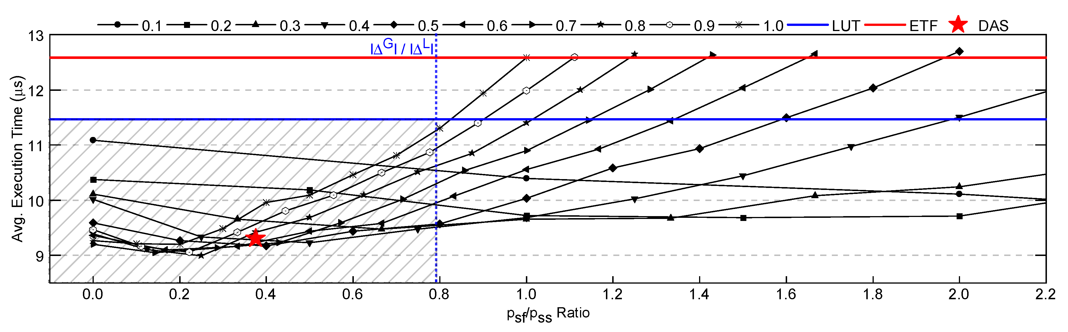
Figure A2. Experimental results that shows average execution time for different

p_{s f} / p_{s s}

ratios. Fast and slow scheduler results are also shown in the figure using straight lines. It also shows the DAS preselection classifier model used in Appendix 4 as a point in a red star shape. The shaded region is where the expected trained model results should be.

Figure A2. Experimental results that shows average execution time for different

p_{s f} / p_{s s}

In order to utilize the equations discussed in Appendix A.1, it is necessary to determine the ideal scheduler decisions and compute the

Δ^{L}

and

Δ^{G}

values, which is outlined in Algorithm A1. For each ready task

T_{i}

, the algorithm checks if the decisions of fast and slow schedulers are identical. If this is the case, the ideal scheduler decision for

T_{i}

is the fast scheduler because it incurs a lower overhead for the same decision. If the decisions of fast and slow schedulers are different, the algorithm employs the decision of the slow scheduler for

T_{i}

and the fast scheduler for all other remaining tasks until the end of the simulation,

e x e - n

. Following the simulation, the algorithm compares the execution time of the simulation,

t_{e x e - n}

, to that of

t_{f a s t - n}

, which utilizes the decisions of the fast scheduler for all tasks. If

t_{e x e - n}

is less than

t_{f a s t - n}

, it implies that the ideal scheduler decision for

T_{i}

is the slow scheduler as it yielded better performance than the fast scheduler. Furthermore, the algorithm adds

t_{e x e - n} - t_{f a s t - n}

Δ^{G}

since it represents the gain in the total execution time. If

t_{e x e - n}

is greater than

t_{f a s t - n}

, the ideal scheduler decision for

T_{i}

is the fast scheduler since utilizing the slow scheduler resulted in a higher execution time. For this scenario, the algorithm adds

t_{e x e - n} - t_{f a s t - n}

Δ^{L}

since it represents the loss in the total execution time.

We used the applications listed in Table 2 for the simulations. The simulations were repeated for ten trials of five data rates to account for runtime variations, scheduling approximately 125,000 tasks each run. After the simulations, we calculated the

| Δ^{G} | / | Δ^{L} |

ratio to be 0.793. Therefore, we must demonstrate that a DAS preselection scheduler with a

p_{s f} / p_{s s}

ratio less than 0.793 would outperform the fast scheduler.

Appendix A.2.2. Validating the DAS Framework Superiority

We conducted a comprehensive set of simulations to verify the validity of Equation A4d for the DAS preselection classifier by varying the

p_{s s}

and

p_{s f}

values. We incremented the probability values by 10% in these simulations and performed 121 simulations, with five iterations per

p_{s s}

and

p_{s f}

combination. This resulted in approximately 12,500 scheduled tasks per data point. Figure A2 presents the average execution time with an extensive sweep of the parameters

p_{s s}

and

p_{s f}

. The figure shows an overall trend of increasing execution time when

p_{s f}

increases while

p_{s s}

remains the same. The reason for the increasing execution time is that using a slow scheduler instead of its fast counterpart results in additional overhead. Similarly, when we decrease

p_{s s}

while keeping

p_{s f}

the same, we see a trend of increasing execution time. The plot also includes the results of slow and fast schedulers as solid lines and the empirically found delta ratio as a dashed vertical line. In the region where the

p_{s f} / p_{s s}

ratio is less than 0.793, the lines are always in the shaded area. This indicates that whenever the relation in Equation A4c holds, the execution time is always better than that achieved with the fast scheduler and, therefore, better than the slow scheduler in Region-2. Thus, for a trained DAS preselection classifier model to guarantee outperforming both schedulers, the

p_{s f} / p_{s s}

ratio must be less than 0.793. We analyzed the performance of the trained DAS preselection classifier model used in Appendix 4 and included a star-shaped point in Figure A2 to represent it. Our trained DAS preselection classifier model has a

p_{s f} / p_{s s}

ratio of 0.376. Therefore, our DAS framework is guaranteed to perform better than both schedulers as its

p_{s f} / p_{s s}

ratio is less than the threshold.

Appendix B. DSSoC Simulator Workload Mixes

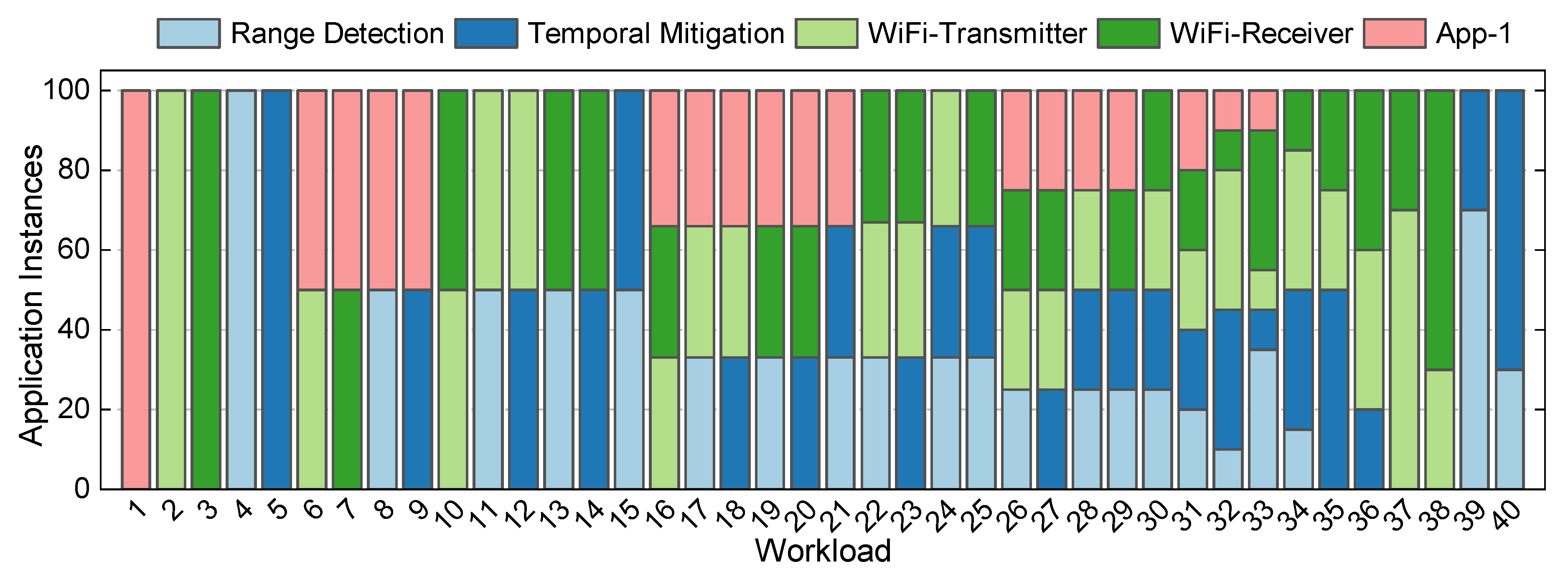
Figure A3 presents the workload mixes used in the DSSoC simulator. Each workload consists of 100 jobs and the stacked bar for each workload denotes the number of instances of each type of application. For instance, Workload-6 (WKL-6) uses 50 instances of WiFi-Transmitter and 50 instances of App-1, and Workload-31 (WKL-31) uses 20 instances of each type. The distribution is selected so that it represents a variety of low, medium, and high data rates.

Figure A3. The distribution of number and type of application instances in the 40 workloads used for evaluation of the DAS framework on the DSSoC simulator.

Appendix C. Runtime Framework Workload Mixes

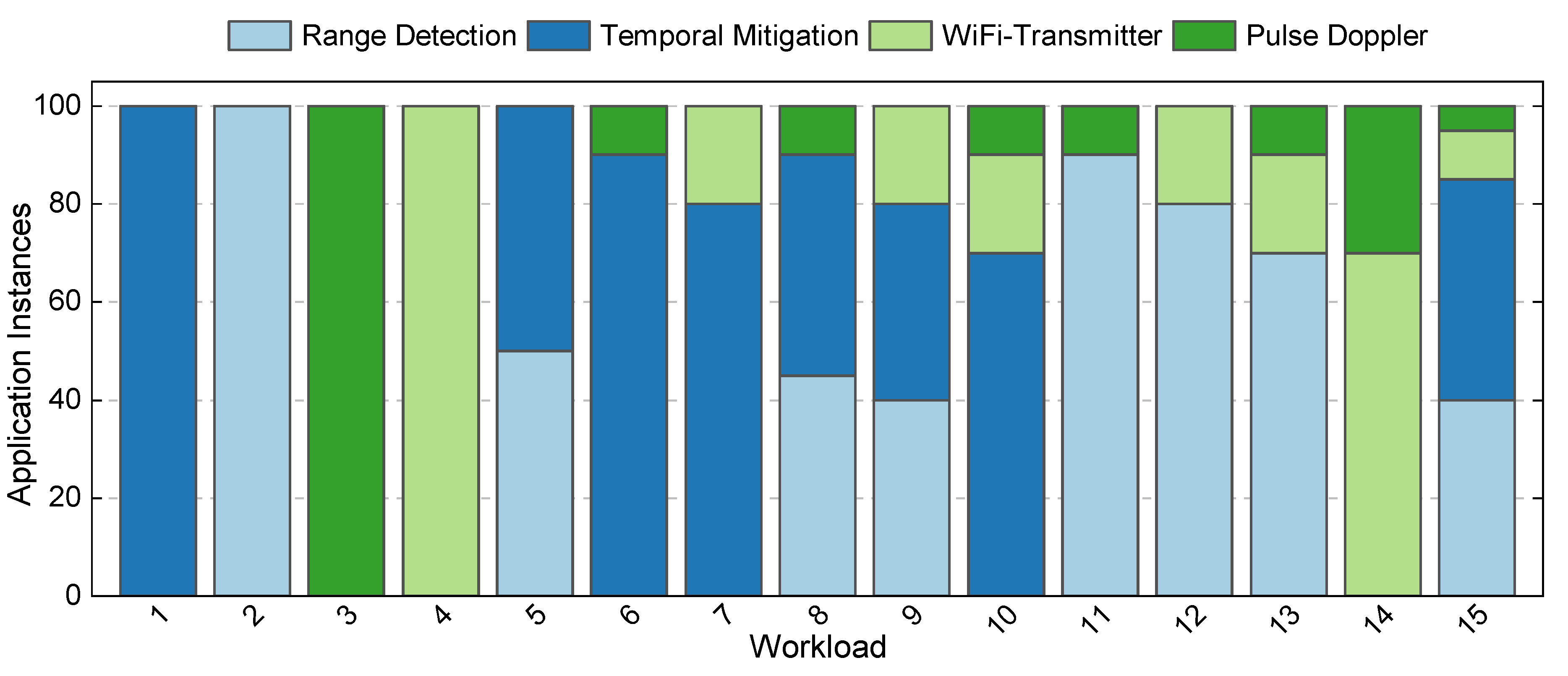
Figure A4 presents the workload mixes used in the DSSoC simulator. Each workload consists of 100 jobs, and the stacked bar for each workload denotes the number of instances of each type of application. For example, Workload-7 (WKL-7) uses 80 instances of Temporal Mitigation and 20 instances of WiFi-Transmitter, and Workload-14 (WKL-14) uses 30 instances of Pulse Doppler and 70 instances of WiFi-Transmitter. The distribution is selected so that it represents a variety of low, medium, and high data rates. Also, we try to balance the distribution of applications. For example, the Pulse Doppler application has highly parallel FFT tasks which dominate the system. Therefore, we try to minimize the number of Pulse Doppler instances. Otherwise, the system is overwhelmed by the FFT tasks from a few instances of Pulse Doppler.

Figure A4. The distribution of number and type of application instances in the 15 workloads used for evaluation of the DAS framework on the runtime framework.

References

Goksoy, A.A.; Krishnakumar, A.; Hassan, M.S.; Farcas, A.J.; Akoglu, A.; Marculescu, R.; Ogras, U.Y. DAS: Dynamic adaptive scheduling for energy-efficient heterogeneous SoCs. IEEE Embedded Systems Letters 2021, 14, 51–54. [Google Scholar] [CrossRef]
Hennessy, J.L.; Patterson, D.A. A New Golden Age for Computer Architecture. Commun. of the ACM 2019, 62, 48–60. [Google Scholar] [CrossRef]
Green, D.; et al. Heterogeneous Integration at DARPA: Pathfinding and Progress in Assembly Approaches. ECTC, 2018. [Google Scholar]
RF Convergence: From the Signals to the Computer by Dr. Tom Rondeau (Microsystems Technology Office, DARPA). https://futurenetworks.ieee.org/images/files/pdf/FirstResponder/Tom-Rondeau-DARPA.pdf. [Online; last accessed 19-March-2023.].
Moazzemi, K.; Maity, B.; Yi, S.; Rahmani, A.M.; Dutt, N. HESSLE-FREE: Heterogeneous Systems Leveraging Fuzzy Control for Runtime Resource Management. ACM Transactions on Embedded Computing Systems (TECS) 2019, 18, 1–19. [Google Scholar] [CrossRef]
Mack, J.; Hassan, S.; Kumbhare, N.; Gonzalez, M.C.; Akoglu, A. CEDR-A Compiler-integrated, Extensible DSSoC Runtime. ACM Transactions on Embedded Computing Systems (TECS) 2022. [Google Scholar] [CrossRef]
Magarshack, P.; Paulin, P.G. System-on-chip Beyond the Nanometer Wall. In Proceedings of the Design Automation Conference; 2003; pp. 419–424. [Google Scholar]
Choi, Y.K.; et al. In-depth Analysis on Microarchitectures of Modern Heterogeneous CPU-FPGA Platforms. ACM Transactions on Reconfigurable Technology and Systems 2019, 12, 1–20. [Google Scholar] [CrossRef]
Krishnakumar, A.; Ogras, U.; Marculescu, R.; Kishinevsky, M.; Mudge, T. Domain-Specific Architectures: Research Problems and Promising Approaches. ACM Transactions on Embedded Computing Systems 2023, 22, 1–26. [Google Scholar] [CrossRef]
Krishnakumar, A.; et al. Runtime Task Scheduling using Imitation Learning for Heterogeneous Many-core Systems. IEEE Trans. CAD Integr. Circuits Syst. 2020, 39, 4064–4077. [Google Scholar] [CrossRef]
Pabla, C.S. Completely Fair Scheduler. Linux Journal 2009. [Google Scholar]
Beisel, T.; Wiersema, T.; Plessl, C.; Brinkmann, A. Cooperative Multitasking for Heterogeneous Accelerators in the Linux Completely Fair Scheduler. In Proceedings of the IEEE International Conference on Application-Specific Systems, Architectures and Processors; 2011; pp. 223–226. [Google Scholar]
Arda, S.E.; et al. DS3: A System-Level Domain-Specific System-on-Chip Simulation Framework. IEEE Trans. Computers 2020, 69, 1248–1262. [Google Scholar] [CrossRef]
Zynq ZCU102 Evaluation Kit. https://www.xilinx.com/products/boards-and-kits/ek-u1-zcu102-g.html, Accessed 10 March 2023.
Topcuoglu, H.; Hariri, S.; Wu, M.Y. Performance-Effective and Low-Complexity Task Scheduling for Heterogeneous Computing. IEEE Trans. on Parallel and Distrib. Syst. 2002, 13, 260–274. [Google Scholar] [CrossRef]
Bittencourt, L.F.; Sakellariou, R.; Madeira, E.R. DAG Scheduling Using a Lookahead Variant of the Heterogeneous Earliest Finish Time Algorithm. In Proceedings of the IEEE Euromicro Conf. on Parallel, Distrib. and Network-based Process. 2010; pp. 27–34. [Google Scholar]
Vasile, M.A.; Pop, F.; Tutueanu, R.I.; Cristea, V.; Kołodziej, J. Resource-Aware Hybrid Scheduling Algorithm in Heterogeneous Distributed Computing. Future Generation Computer Systems 2015, 51, 61–71. [Google Scholar] [CrossRef]
Yang, H.; Ha, S. ILP based data parallel multi-task mapping/scheduling technique for MPSoC. In Proceedings of the 2008 International SoC Design Conference; 2008; Volume 1, pp. 1–134. [Google Scholar]
Benini, L.; Bertozzi, D.; Milano, M. Resource Management Policy Handling Multiple Use-Cases in MpSoC Platforms using Constraint Programming. In Proceedings of the Logic Programming: 24th International Conference, ICLP 2008, Udine, Italy, 9-13 December 2008; 2008; pp. 470–484. [Google Scholar]
Yoo, A.B.; Jette, M.A.; Grondona, M. Slurm: Simple Linux Utility for Resource Management. In Proceedings of the Workshop on Job Scheduling Strategies for Parallel Processing; 2003; pp. 44–60. [Google Scholar]
Thain, D.; Tannenbaum, T.; Livny, M. Distributed computing in practice: the Condor experience. Concurrency and Computation: Practice and Experience 2005, 17, 323–356. [Google Scholar] [CrossRef]
Chronaki, K.; et al. Task Scheduling Techniques for Asymmetric Multi-core Systems. IEEE Trans. on Parallel and Distrib. Systems 2016, 28, 2074–2087. [Google Scholar] [CrossRef]
Zhou, J. Real-time Task Scheduling and Network Device Security for Complex Embedded Systems based on Deep Learning Networks. Microprocessors and Microsystems 2020, 79, 103282. [Google Scholar] [CrossRef]
Namazi, A.; Safari, S.; Mohammadi, S. CMV: Clustered Majority Voting Reliability-aware Task Scheduling for Multicore Real-time Systems. IEEE Trans. on Reliability 2018, 68, 187–200. [Google Scholar] [CrossRef]
Xie, G.; Zeng, G.; Liu, L.; Li, R.; Li, K. Mixed Real-Time Scheduling of Multiple DAGs-based Applications on Heterogeneous Multi-core Processors. Microprocessors and Microsystems 2016, 47, 93–103. [Google Scholar] [CrossRef]
Xiaoyong, T.; Li, K.; Zeng, Z.; Veeravalli, B. A Novel Security-Driven Scheduling Algorithm for Precedence-Constrained Tasks in Heterogeneous Distributed Systems. IEEE Transactions on Computers 2010, 60, 1017–1029. [Google Scholar] [CrossRef]
Kwok, Y.K.; Ahmad, I. Dynamic Critical-Path Scheduling: An Effective Technique for Allocating Task Graphs to Multiprocessors. IEEE Trans. Parallel Distrib. Syst. 1996, 7, 506–521. [Google Scholar] [CrossRef]
Sakellariou, R.; Zhao, H. A Hybrid Heuristic for DAG Scheduling on Heterogeneous Systems. In Proceedings of the Int. Parallel and Distributed Processing Symposium; 2004; p. 111. [Google Scholar]
Jejurikar, R.; Gupta, R. Energy-aware Task Scheduling with Task Synchronization for Embedded Real-time Systems. IEEE Trans. CAD of Integr. Circuits Syst. 2006, 25, 1024–1037. [Google Scholar] [CrossRef]
Azad, P.; Navimipour, N.J. An Energy-aware Task Scheduling in the Cloud Computing using a Hybrid Cultural and Ant Colony Optimization Algorithm. Int. Journal of Cloud Applications and Computing 2017, 7, 20–40. [Google Scholar] [CrossRef]
Baskiyar, S.; Abdel-Kader, R. Energy Aware DAG Scheduling on Heterogeneous Systems. Cluster Computing 2010, 13, 373–383. [Google Scholar] [CrossRef]
Swaminathan, V.; Chakrabarty, K. Real-Time Task Scheduling for Energy-Aware Embedded Systems. Journal of the Franklin Institute 2001, 338, 729–750. [Google Scholar] [CrossRef]
Streit, A. A Self-tuning Job Scheduler Family with Dynamic Policy Switching. In Proceedings of the Workshop on Job Scheduling Strategies for Parallel Process; 2002; pp. 1–23. [Google Scholar]
Daoud, M.I.; Kharma, N. A Hybrid Heuristic–genetic Algorithm for Task Scheduling in Heterogeneous Processor Networks. Journal of Parallel and Distrib. Computing 2011, 71, 1518–1531. [Google Scholar] [CrossRef]
Boeres, C.; Lima, A.; Rebello, V.E. Hybrid Task Scheduling: Integrating Static and Dynamic Heuristics. In Proceedings of the Proc. of 15th Symp. on Computer Arch. and High Perform. Computing; 2003; pp. 199–206. [Google Scholar]
McHugh, M.L. The Chi-square Test of Independence. Biochemia Medica 2013, 23, 143–149. [Google Scholar] [CrossRef] [PubMed]
Hwang, J.J.; Chow, Y.C.; Anger, F.D.; Lee, C.Y. Scheduling Precedence Graphs in Systems with Interprocessor Communication Times. SIAM Journal on Computing 1989, 18, 244–257. [Google Scholar] [CrossRef]
ZeBu server 4. https://www.synopsys.com/verification/emulation/zebu-server.html. accessed date: Jan. 2, 2020.
Veloce2 emulator. https://www.mentor.com/products/fv/emulation-systems/veloce. accessed date: Jan. 2, 2020.
Mack, J.; Kumbhare, N.; NK, A.; Ogras, U.Y.; Akoglu, A. User-Space Emulation Framework for Domain-Specific SoC Design. In Proceedings of the 2020 IEEE Int. Parallel and Distrib. Process. Symp. Workshops; 2020; pp. 44–53. [Google Scholar]
Xilinx - Accurate Power Measurement. https://www.xilinx.com/developer/articles/accurate-design-power-measurement.html. accessed date: Feb. 11, 2023.
Sysfs Interface in Linux. https://www.kernel.org/doc/Documentation/hwmon/sysfs-interface. accessed date: Feb. 11, 2023.

Figure 1. An example of the relationship of (a) execution time and (b) energy-delay product (EDP) between simple low-overhead (lookup table or LUT) and sophisticated high-overhead schedulers.

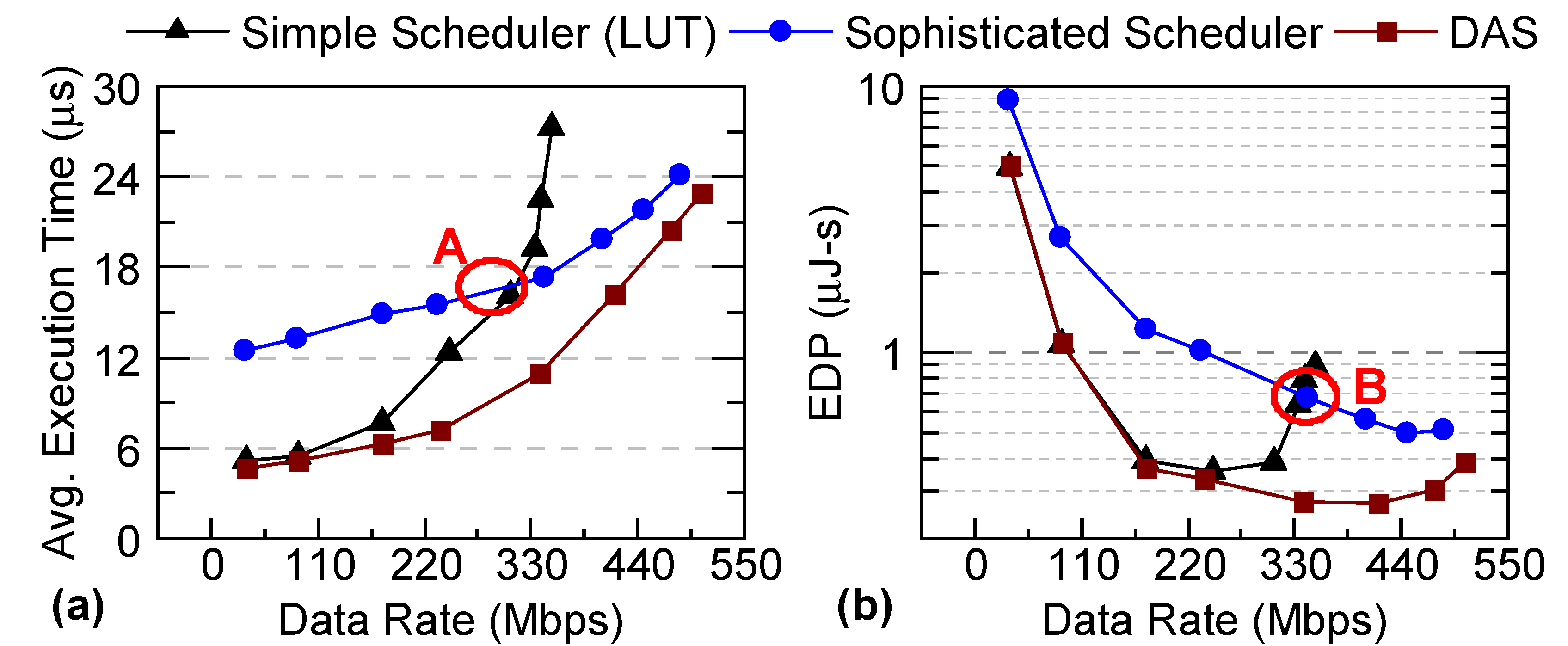
Figure 2. Flowchart describing the construction of an Oracle to dynamically choose the best-performing scheduler at runtime.

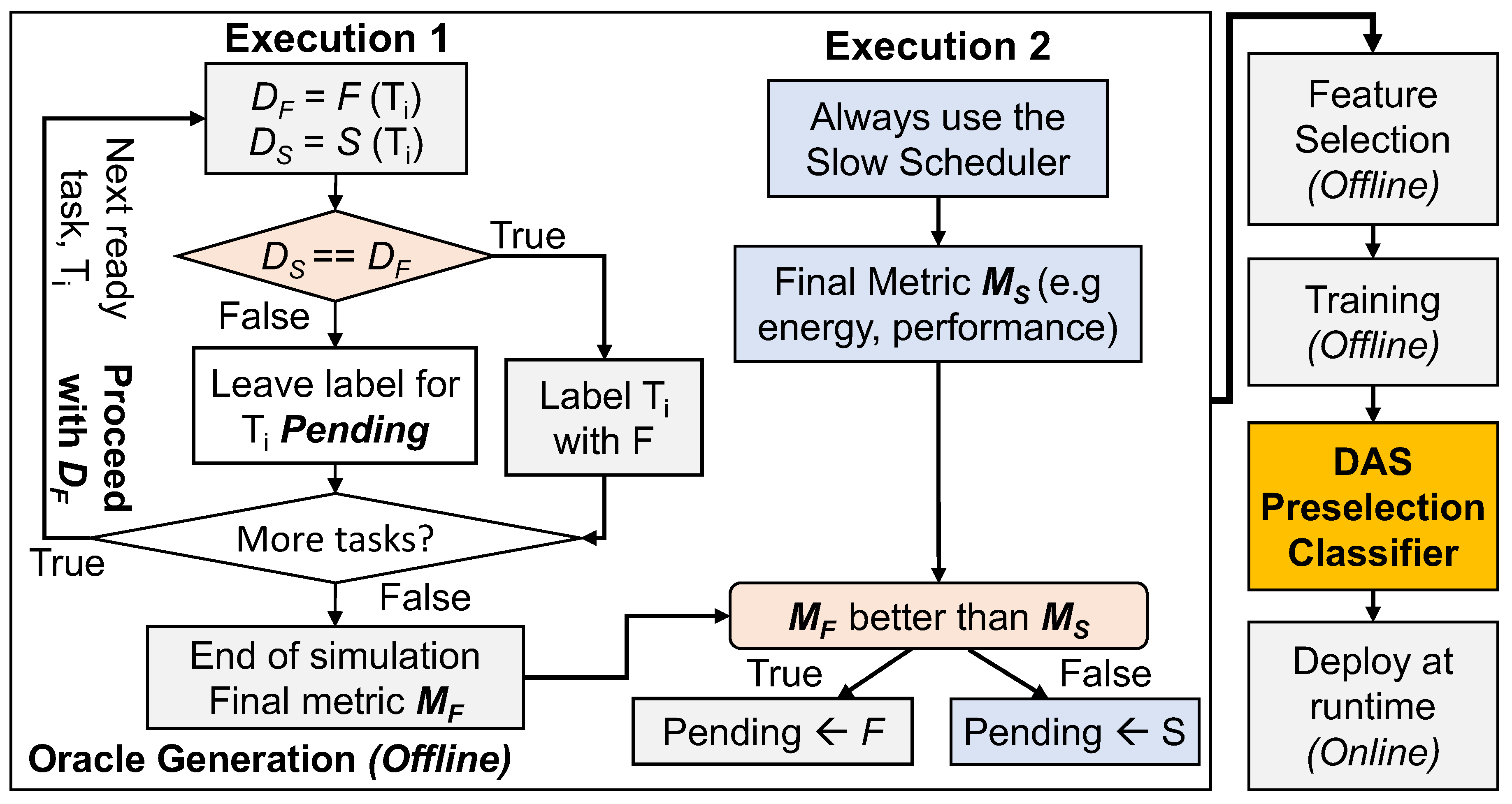
Figure 3. ETF scheduling overhead and fitted quadratic curve.

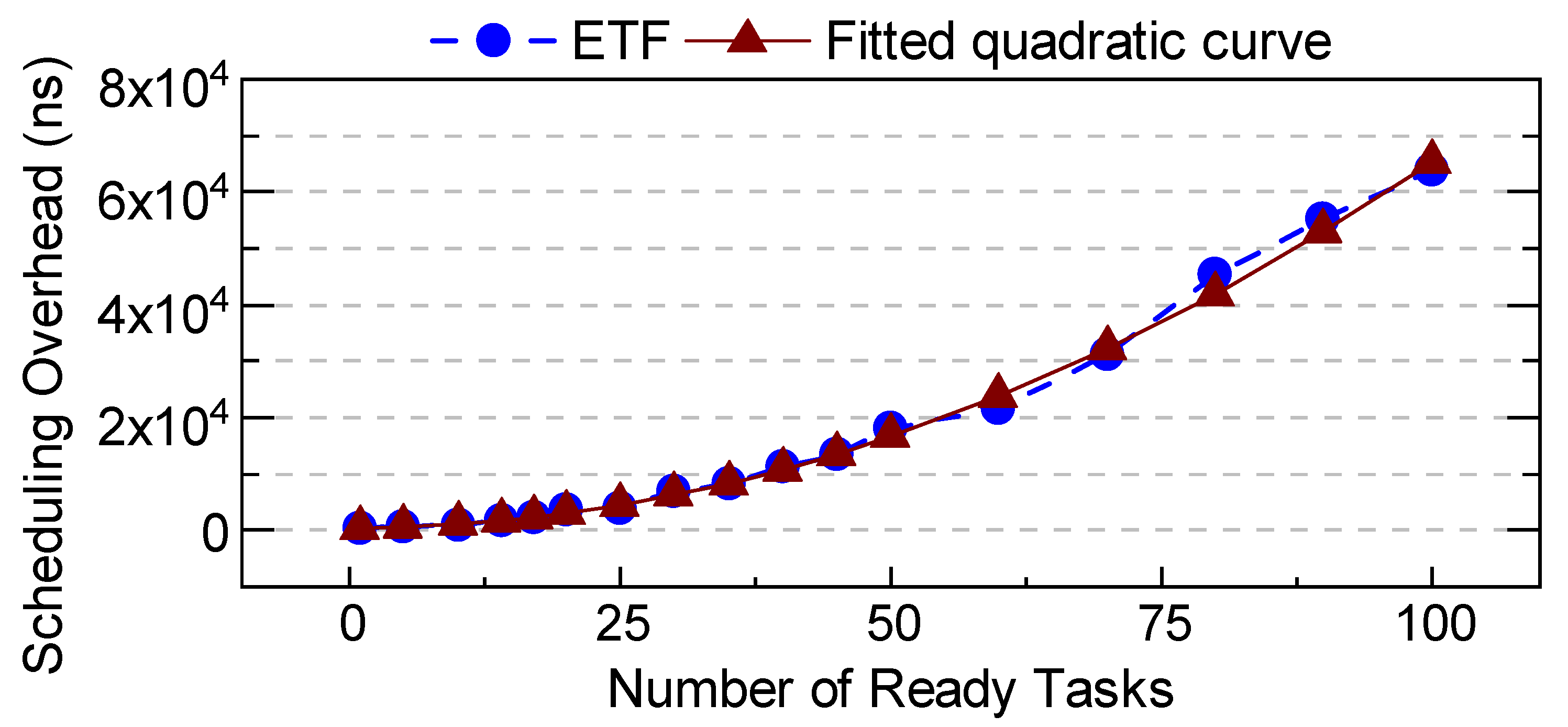
Figure 4. A comparison of average execution time (a–c) and energy-delay product (EDP) (d–f) between DAS, lookup table (LUT), earliest task first (ETF) and ETF-ideal for three different workloads.

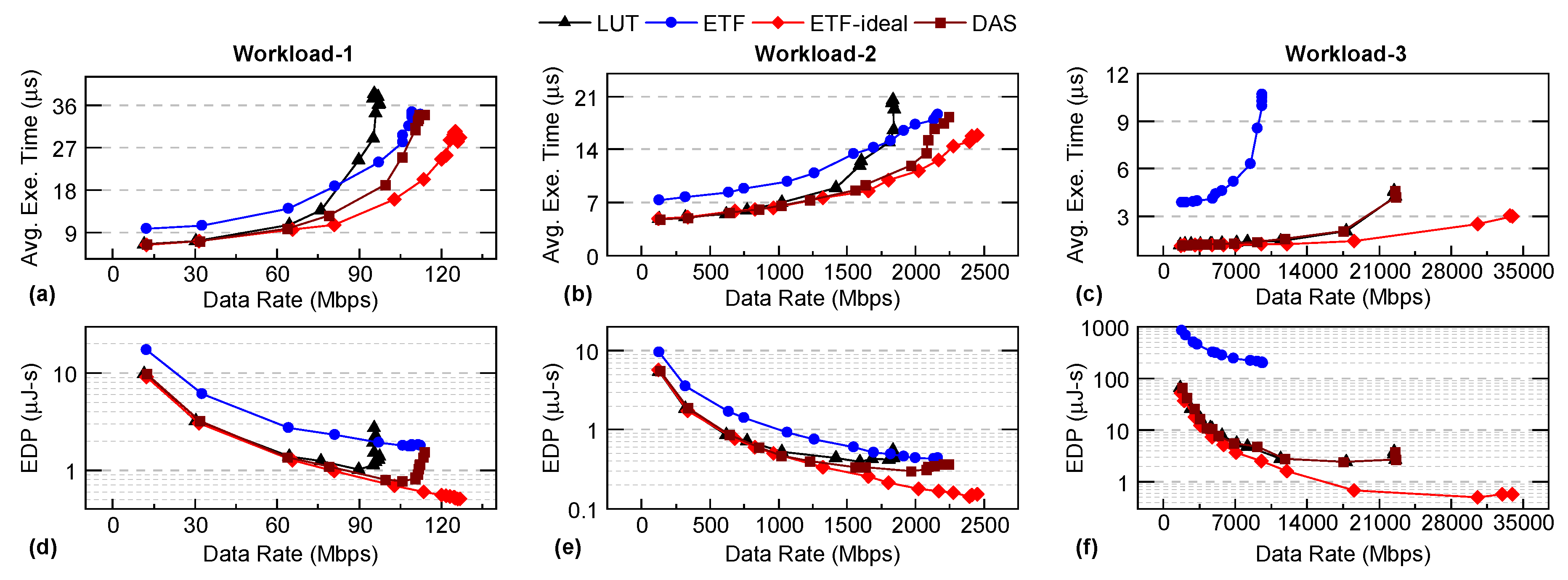
Figure 5. A comparison of average job slowdown of between DAS, LUT, and ETF for twenty five workloads.

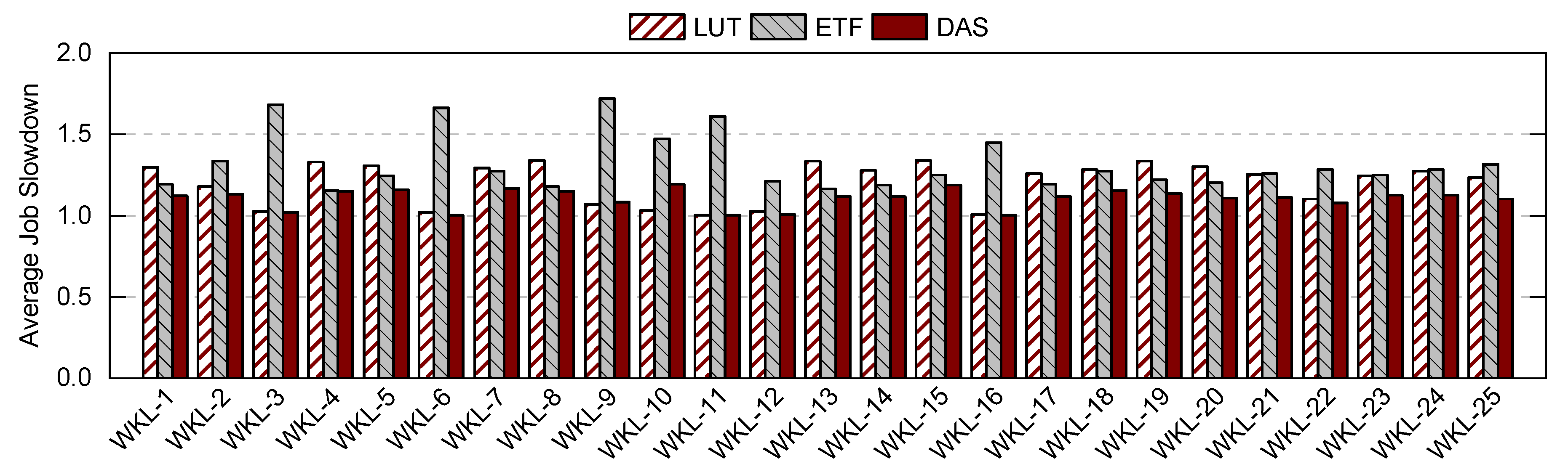
Figure 6. A comparison of average execution time between DAS, LUT, ETF, ETF-ideal, and the heuristic approach.

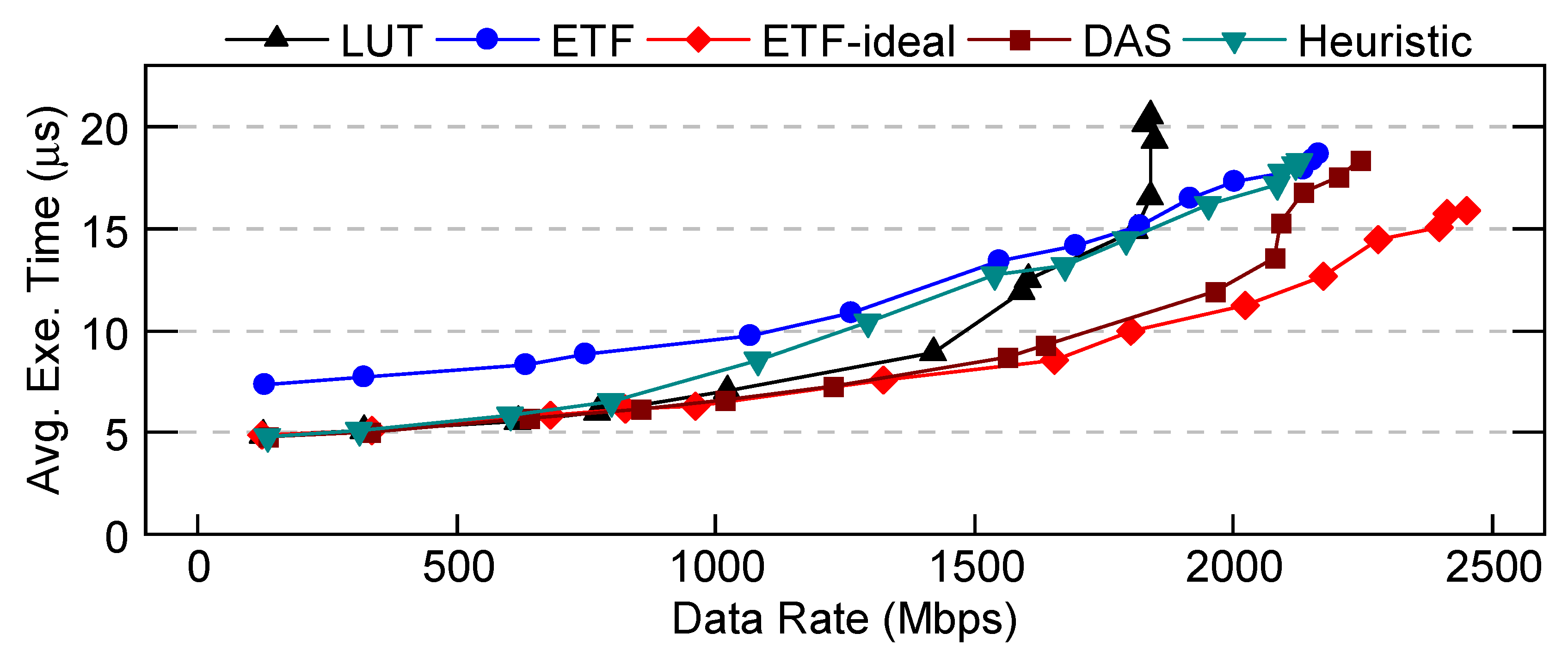
Figure 7. Decisions taken by the DAS framework as bar plots and total scheduling energy overheads of LUT, ETF and DAS as line plots.

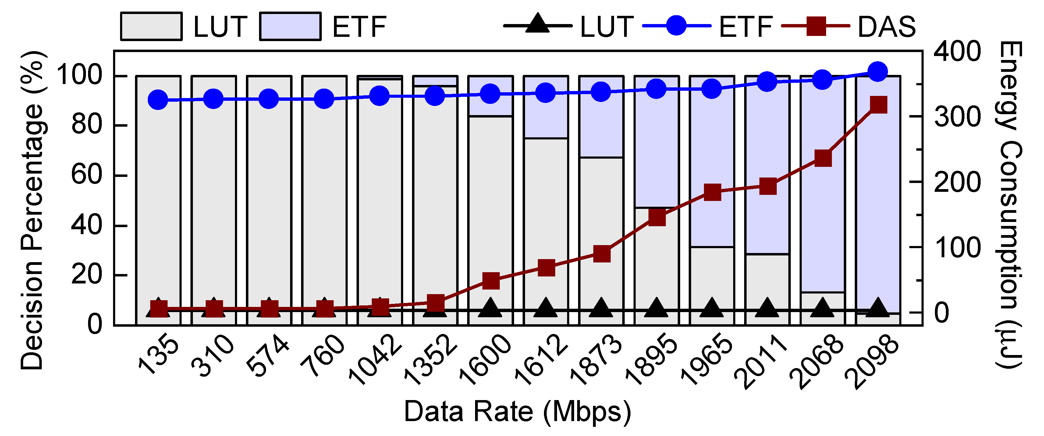
Figure 8. A comparison of average execution time (a–c) and energy-delay product (EDP) (d–f) between DAS, LUT, ETF on a hardware platform for three different workloads.

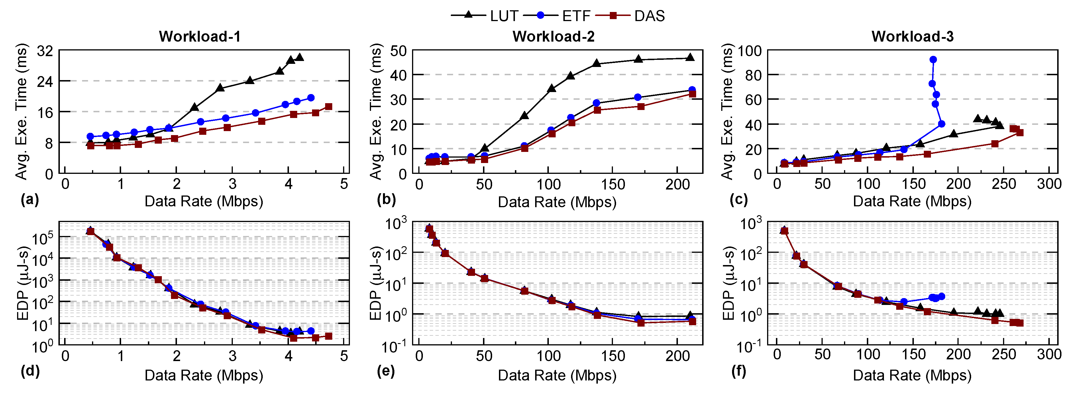
Table 1. Type of performance counters used by DAS for system state representation and runtime classification between schedulers.

Type	Features
Task	Task ID, Execution time, Power consumption, Depth of task in DFG, Application ID, Predecessor task ID and cluster IDs, Application type
Processing Element (PE)	Earliest time when PE is ready to execute, Earliest availability time of each cluster, PE utilization, Communication cost
System	Input data rate

Table 2. Characteristics of applications from radar processing and wireless communication domains used in this study. (FFT=fast Fourier transform, FEC=forward error correction, FIR=finite impulse response, SAP=systolic array processor)

Application	Number of Tasks	Supported Clusters
Range Detection	7	big, LITTLE, FFT, SAP
Temporal Mitigation	10	big, LITTLE, FIR, SAP
WiFi-TX	27	big, LITTLE, FFT, SAP
WiFi-RX	34	big, LITTLE, FFT, FEC, FIR, SAP
App-1	10	LITTLE, FIR, SAP

Table 3. DSSoC configuration used for DAS evaluation

Processing Cluster	No. of Cores	Functionality
LITTLE	4	General-purpose
big	4	General-purpose
FFT	4	Acceleration of FFT
FEC	1	Acceleration of encoding and decoding operations
FIR	4	Acceleration of FIR
SAP	2	Multi-function acceleration
TOTAL	19

Table 4. Classification accuracies and storage overhead of DAS models with different machine learning classifiers and features

Classifier	Tree Depth	Number of Features	Classification Accuracy (%)	Storage (KB)
LR	-	2	79.23	0.01
LR	-	62	83.1	0.24
DT	2	1	63.66	0.01
DT	2	2	85.48	0.01
DT	3	6	85.51	0.03
DT	2	62	85.9	0.01
DT	16	62	91.65	256

Disclaimer/Publisher’s Note: The statements, opinions and data contained in all publications are solely those of the individual author(s) and contributor(s) and not of MDPI and/or the editor(s). MDPI and/or the editor(s) disclaim responsibility for any injury to people or property resulting from any ideas, methods, instructions or products referred to in the content.

© 2023 by the authors. Licensee MDPI, Basel, Switzerland. This article is an open access article distributed under the terms and conditions of the Creative Commons Attribution (CC BY) license (http://creativecommons.org/licenses/by/4.0/).

Copyright: This open access article is published under a Creative Commons CC BY 4.0 license, which permit the free download, distribution, and reuse, provided that the author and preprint are cited in any reuse.

Downloads

127

Views

Comments

Subscription

Notify me about updates to this article or when a peer-reviewed version is published.

MDPI Initiatives

Important Links

Choose an area of interest and we will send you notifications of new preprints at your preferred frequency.

Disclaimer

Theoretical Validation and Hardware Implementation of Dynamic Adaptive Scheduling for Heterogeneous Systems-on-Chip

Abstract

Keywords:

Subject:

1. Introduction

2. Related Work

3. Dynamic Adaptive Scheduling Framework

3.1. Overview and Preliminaries

3.2. DAS Preselection Classifier

3.3. Fast & Slow (F&S) Scheduler Selection

4. Evaluation of DAS Using Simulations

4.1. Simulation Setup

4.2. Exploration of Machine Learning Techniques and Feature Space for DAS

4.3. Performance Analysis for Different Workloads

4.4. Scheduling Overhead and Energy Consumption Analysis

5. Evaluation of DAS using FPGA Emulation

5.1. Experimental Setup

5.2. Performance Results

6. Conclusions

Author Contributions

Funding

Institutional Review Board Statement

Informed Consent Statement

Data Availability Statement

Conflicts of Interest

Appendix A. Theoretical Proof for DAS Framework

Appendix A.1. Necessary Conditions for the Superiority of DAS

Appendix A.2. Experimental Validation of the Proof

Appendix A.2.1. Finding the Empirical Values for Δ L and Δ G

Appendix A.2.2. Validating the DAS Framework Superiority

Appendix B. DSSoC Simulator Workload Mixes

Appendix C. Runtime Framework Workload Mixes

References

MDPI Initiatives

Important Links

Subscribe