Submitted:
30 August 2023
Posted:
31 August 2023
You are already at the latest version
Abstract
An automatic recognizing system of white blood cells can assist hematologists in the diagnosis of many diseases, where accuracy and efficiency are paramount for computer-based system. In this paper, we present a new image processing system to recognize the five types of white blood cells in peripheral blood with marked improvement in efficiency when juxtaposed against mainstream methods. The prevailing deep learning segmentation solutions often utilize millions of parameters to extract high-level image features and neglect the incorporation of prior domain knowledge, which consequently consume substantial computational resources and increase the risk of overfitting, especially when limited medical image samples are available for training.
To address these challenges, we propose a novel memory-efficient strategy that exploits graph structures derived from the images.
Specifically, we introduce a lightweight superpixel-based Graph Neural Network (GNN) and break new ground by introducing superpixel metric learning to segment nucles and cytoplasm. Remarkably, our proposed segmentation model (SMGNN) achieves state-of-the-art segmentation performance while utilizing at most 10000$\times$ less than the parameters compared to existing approaches. The subsequent segmentation-based cell type classification processes show satisfactory results that such automatic recognizing algorithms are accurate and efficient to execeute in hematological laboratories.
Keywords:
Graph Neural Networks
; Superpixel metric learning
; Memory efficient model
; White blood cell segmentation
; Cell type classification
0. Introduction
White blood cells (WBCs), also known as leukocytes, play a pivotal role in the immune system’s defense against various infections. Accurate quantification and classification of WBCs can provide valuable insights for diagnosing a wide range of diseases, including infections, leukemia [1], and AIDS [2]. In the laboratory environment, the traditional examination of blood smears was a laborious and time-consuming manual task. However, with the advent of computer-aided automatic cell analysis systems, rapid and high-throughput image analysis tasks can now be accomplished [3]. This automated system typically entails three major steps: image acquisition, cell segmentation, and cell type classification. Among these steps, cell segmentation is widely recognized as the most crucial and challenging one, as it significantly influences the accuracy and computational complexity of subsequent processes [4].
Accurately segmenting WBCs in cell images, thereby distinguishing between lymphocytes, monocytes, eosinophils, basophils, and neutrophils as shown in Figure 1, provides a wealth of crucial information for hematological diagnostics [5,6]. However, capturing these images necessitates meticulous attention to factors such as image resolution, exposure duration, illumination levels, and the appropriate use of optical filters. Suboptimal choices in imaging technology or parameters can compromise image quality, presenting challenges for white blood cell image analyses.
Deep learning, particularly convolutional neural networks (CNNs), has revolutionized medical image segmentation. U-Net [7], a symmetrical encoder-decoder convolutional network featuring skip connections, stands as a prime example. Subsequent iterations, like U-Net++ [8], U-Net3+ [9], and RU-Net [10], have enhanced its capabilities. Parallelly, Transformer-based approaches, such as Vision Transformer (ViT) [11] and Swin Transformer [12], have emerged, leveraging self-attention mechanisms for better feature extraction. Specifically, the ViT partitions images into non-overlapping patches and treats the patches as sequence data, where the self-attention mechanism is subsequently used to extract long-range information among patches. Furthermore, the Swin Transformer applies a shifted window to make ViT more computationally efficient. Though ViT exhibits significantly better performance on large objects, it obtains lower performance on small objects [13]. This may be caused by the fixed scale of patches generated by Transformer-based methods. Notably, U-Net architectures have also incorporated transformers, yielding U-Net Transformer [14], Medical Transformer [15], and Swin-Unet [16]—all of which have set new performance benchmarks in medical image segmentation. However, these architectures, rooted in pixel-based learning, demand substantial memory resources, leading to inefficiencies, especially when available training samples are scanty [17]. Here, large models might face narrowing expressivity gaps against parameter-efficient counterparts. To mitigate this, embedding prior knowledge can reduce the computational burden.
Graph structure data provides an elegant way of describing the geometry of data, which contains abundant relational information. For example, diverse types of relational systems or structured entities can be described by graphs to include the interior connections, where some typical examples include particle system analysis [18,19], social networks [20], and molecular properties prediction [21]. Correspondingly, graph neural networks (GNNs) are specifically designed to process graph data [22,23,24,25,26], where researchers have developed graph convolutional networks (GCNs) and various variants to update node features by aggregating information from neighboring nodes.
The transformation of image data, particularly those without an inherent geometric structure, into graph data, represents a substantial challenge. This challenge is twofold: encoding Euclidean space data into graph representations and decoding them back to their original image domain. A prevalent approach to address this involves the use of a patch graph method, where image patches are treated as graph nodes. For example, the Graph-FCN [27] applies a fully convolutional network (FCN) to extract image features, and the graph structure is constructed based on the k nearest neighbor (kNN) methods where the weight adjacent matrix is generated with the Gaussian kernel function. In [28], the dual graph convolution network (DGCNet) constructs the graph structure not only on the spatial domain but also on the feature domain. In the semantic segmentation task, the bilinear interpolation upsampling operation acted on the down-sampled output of the DGCNet to recover the same image size as the label.
However, while the patch-based method offers convenience in graph construction, it has its limitations. The fixed structure of image patches can lead to the omission of critical boundary details. An alternative lies in the superpixel approach. Superpixels, by design, can dramatically lower both computational and memory costs for image processing. Since image superpixel can significantly reduce the computational and memory overhead for image processing tasks, superpixel methods are commonly implemented as a pre-processing step before the deep reasoning models [29,30,31,32,33,34,35,36]. Various superpixel methods over-segment the image into multiple non-overlapped regions based on the pixel features and homogeneous pixels are grouped inside single superpixel. Traditional superpixel generation method can be roughly divided into graph-based [37,38,39] and clustering-based [40,41,42,43] methods. These methods are efficient and fast to generate high-quality superpixels and require no human label and less memory in computing. Recently, the deep learning based approaches are employed in superpixel sampling [44,45,46,47,48]. These methods are accurate but not efficient in memory saving since learning high-level image features requires a relatively large amount of convolution kernel parameters. Based on the pre-computed superpixel graph and graph neural network, [49] captures global feature interactions for brain tumor segmentation. In [50], superpixel-based graph data and edge-labeling graph neural network (EGNN) [51] are implemented for biological image segmentation.
Medical image segmentation has long depended on the precision achieved by supervised learning methods. Yet, the perennial issue remains, that is the paucity of richly labeled datasets in clinical contexts. This limitation has driven the pivot to metric learning, which disrupts the entrenched belief that robust intelligence is the sole preserve of abundant labeled data [52,53,54,55]. Metric learning approaches, such as contrastive methods, learn representations in a discriminative manner by contrasting positive sample pairs against negative pairs. By tapping into vast reservoirs of unlabeled samples, they set the stage for pretraining deep learning models. The subsequent phase involves meticulous fine-tuning, utilizing just a fraction of labeled samples. Remarkably, the outcome is a model performance that stands shoulder to shoulder with traditional supervised strategies. Notably, there’s a burgeoning interest in supervised metric learning methods, specifically tailored to unravel cross-image intricacies. These techniques use sample labels as the blueprint to categorize them into positive and negative sets [56]. The confluence of metric learning methods offers deep learning models a unique advantage. By bridging labeled and unlabeled data, they are empowered to deliver stellar results, even when navigating the constraints of scantily labeled samples.
In this work, we propose a novel approach for white blood cells segmentation, namely Superpixel Metric Graph Neural Network (SMGNN). The core strength of SMGNN lies in its dual promise: delivering unparalleled accuracy while simultaneously optimizing memory efficiency. The foundation of our technique is a superpixel graph constructed from image data. This restructuring drastically diminishes the problem’s dimensionality and serves as a conduit for infusing abundant prior information into the graph data. In addition to leveraging prior knowledge on a single training sample, our proposed approach introduces superpixel metric learning to capture “global” context across the training samples. In clinical image segmentation scenarios with limited training samples, we believe incorporating this “global” context can enhance the expressivity of deep learning models. Our proposed metric learning operates on the superpixel embeddings rather than the vast number of pixel embeddings, which offers the advantage of memory saving.
The contributions of this paper can be summarized as follows.
- Our proposed lightweight superpixel metric graph neural network significantly reduces the learnable parameters by at most 10000 times compared with mainstream segmentation models.
- Our proposed superpixel-based model reduces the problem size and poses rich prior knowledge to the rarely considered graph structure data, which helps SMGNN achieve SOTA performance on white blood cell images.
- We innovatively propose superpixel metric learning according to the definition of superpixel metric score, which is more efficient than pixel-level metric learning.
- The whole deep learning based nucleus and cytoplasm segmentation and cell type classification system is accurate and efficient to execute in hematological laboratories.
The remaining sections of this article are structured as follows. Section 1 describes our methodology in depth. Section 2 depicts the workflow and architecture of our proposed model. In Section 3, through extended segmentation experiments, the SMGNN model achieves state-of-the-art performance in terms of both accuracy and memory efficiency and the five cell types classification task
Figure 2.
The main idea underlying our approach is to learn the distance between superpixel embeddings using the superpixel metric score, which is the ratio of the majority class inside the superpixel. Given the anchor embedding, similar embeddings with approximate metric scores will be pulled close, and dissimilar embeddings will be pushed away. With the help of metric learning, the cross-image global context can be captured and a better embedding space will be learned.

1. Methodolgy of Superpixel Metric
Deep learning methods for medical image processing have predominantly concentrated on discerning the local context, which refers to inter-pixel dependencies within individual images [56]. However, there’s a missed opportunity: capturing the “global” context that exists between training samples. While pixel-level contrast or metric learning provides a way to bridge this gap, the sheer computational and memory overheads—due to contrast or metric computations spanning every pixel pair—render them less feasible. We propose an innovative efficient superpixel-level metric learning on metric loss, which not only captures the desired global context but does so while drastically cutting computational and memory costs.
1.1. Compression Ratio on Image Data
The utility of superpixel methods in image data preprocessing is well-acknowledged, particularly for their ability to condense data and reduce computational demands. Consequently, this study capitalizes on these advantages, transforming the image data into a more compact graph representation. Within this framework, each superpixel evolves into a graph node. The interconnectedness of these nodes—whether driven by spatial positioning or feature similarity—determines the graph’s topology. These node features aren’t rigid; their definition can range from basic 5-dimensional attributes encompassing color (3 dimensions) and location (2 dimensions) to more intricate data points like histograms, positional variance, and variations in pixel values.
Given that the adjacency matrix exhibits sparse characteristics, it’s predominantly the node features that dictate memory consumption. Opting for the more straightforward features facilitates significant data compression. Specifically, for 3-channel RGB images, we’ve discerned a compression ratio roughly represented as . Importantly, this efficient compression does not compromise on quality. Our subsequent numerical experiments demonstrate that this ratio is concomitant with optimal segmentation outcomes.
1.2. Quality of Superpixel and Reconstruction Score
The segmentation task relies on the quality of the generated superpixels, and good superpixel results coherent with the boundary of labeled images. Suppose is the input image. Let be the set of all superpixels, be the number of pixels, be the number of superpixels, and be the association matrix between pixels and superpixels, then we have
where is the jth superpixel, Flatten operation converts a two-dimensional image matrix into a one-dimensional vector. The role of the association matrix build the bridge between image space and graph space. For computation convenience, we define column normalized association matrix as
Let be the label of the image pixels and be superpixel metric or metric score of the graph data. Using the pixel label, we can formulate metric score as
for the superpixel. can also be efficiently computed with column normalized association matrix, i.e., . We can back-project the supepixel label to image space by association matrix, i.e., . We define the IoU reconstruction score to evaluate the quality, which reads
where denotes the set of pixels whose class label equal i, c is the number of classes.
1.3. Lightweight Graph Neural Networks for Superpixel Embedding
Graph neural networks have the advantage of being lightweight compared to other deep learning models that often require deeper and larger networks to achieve higher performance. GNNs leverage relational information and utilize shallow layers to achieve satisfactory results.
Given an undirected attributed graph , consists of a nonempty finite set of nodes and a set of edges between node pairs. Denote the graph adjacency matrix and the node attributes. A graph convolution learns a matrix representation that embeds the structure and feature matrix with for node j. Most graph convolutions follow the message passing [57] update scheme, which finds a central node’s smooth representation by aggregating its 1-hop neighbor information. At layer ℓ, the propagation for the ith node reads
where is a differentiable and permutation invariant aggregation function, such as summation, average, or maximization. The set includes and its 1-hop neighbors. Both and are differentiable aggregation functions, such as MultiLayer Perceptrons (MLPs).
In our approach, we construct graph data using superpixels and their predefined relationships. GNNs learn features from the graph space to enhance the segmentation capability. We employ the Graph Isomorphism Network (GIN) [26] as the backbone graph representation network. At each layer ℓ, the GIN model updates the ith node representation as follows:
where is a learnable weight.
GIN has been proven to possess expressive power equivalent to the 2-Weisfeiler-Lehman test [58]. By utilizing GIN, we can effectively extract informative features from the superpixel graph, enabling accurate and efficient segmentation performance.
1.4. Memory Efficient Metric Learning
Although pixel-wise contrast can learn the global context to form a good segmentation embedding space [56], computing the contrastive loss requires using training image pixels, which leads to a significant amount of computation and memory cost. In this study, we propose superpixel-based methods that can significantly reduce the number of data samples from N to K, and we introduce a memory-efficient distance-based metric loss function.
The fundamental concept of metric learning is to bring similar samples closer together in the embedding space while pushing dissimilar samples further apart. However, pixel-wise contrast methods that involve setting a large number of anchor pixels and using tensor multiplication to compute positive similarity incur high memory costs. To address this, we define the superpixel metric loss using the mean square error (MSE) between the similarity and metric score of the embeddings, as follows:
where and represent the number of anchor samples and reference samples , respectively. Here, d denotes the dimension of the embedding, and a and b are learnable parameters. Additionally, represents the superpixel label of node x, which is defined by Eq. (1). It’s important to note that the anchor/reference samples are not restricted to being from the same image . The objective of Eq. (5) is to bring the embeddings of similar superpixel samples closer together and push dissimilar ones apart.
2. The Work-Flow and Architecture of SMGNN
We use the parameter-free methods to generate superpixels [40,59], on which we construct graph structure with two alternative strategies. Each superpixel is treated as a node and the mean RGB values and mean postion value consist five dimension node features. Suppose the mean scale of superpixels , we can define the adjacency between nodes according to their positional relation as
where and are the positions of superpixel i and superpixel j respectively, and is a hyper-parameter to control the number of neighbouring nodes. The above definition will pose strong local connectivity to the graph data. For batched images, we can use parallel computing to accelerate the graph generation process and then multiple subgraphs combine as a large graph, where only connected nodes can perform message passing with the graph neural networks.
Regarding the model architecture, we utilize three layers of Graph Isomorphism Network to generate the embeddings of superpixels, upon which metric learning is performed. In addition to the transformed graph data derived from superpixels, we retain the original image data. We concatenate the features of superpixels and pixels and pass them through a lightweight convolutional neural network (CNN) to smooth out small pixel groups in the output of the GNNs. This process helps enhance the segmentation accuracy by incorporating non-degraded image information. The overall architecture of our proposed model, named SMGNN, is illustrated in Figure 3.
To tackle the clinical image segmentation, we employ the Dice loss [60], which is a structure-aware and widely used loss function for medical image segmentation. This loss function is designed to measure the similarity between predicted and ground truth segmentation masks. We also use the Dice coefficient to evaluate the performance of different models [60], which a widely used metric on image segmentation. To be more specific, given a set G, we define its characteristic/label function by . The Dice coefficient of two sets G and is defined as
where indicates the domain containing the two sets. The Dice metric is also directly used as loss function to train a supervised segmentation task. The Dice loss function is formulated as
The joint loss function for both the superpixel metric learning and segmentation tasks is defined as a combination of the Dice loss and the superpixel metric loss. This joint loss function enables us to optimize the model parameters simultaneously for both tasks, effectively leveraging the benefits of both superpixel-based metric learning and pixel-wise segmentation. The joint loss function is formulated as
where is a hyperparameter to trade off the learning on image space and graph space.
3. Numerical Experiments
We employed a widely used White Blood Cells dataset to evaluate the effectiveness of our proposed recognizing system. We employed the widely-acclaimed Adam optimization technique [61] for model training during the backpropagation phase. The implementations are programmed with PyTorch-Geometric (ver 2.2.0) and PyTorch (version 1.12.1) and executed on an NVIDIA® Tesla A100 GPU with CUDA cores and 80GB HBM2 installed on an HPC cluster.
3.1. Dataset Description
We verify the robustness of our methods on a small white blood cell image dataset collected from the CellaVision blog 1, which consists of one hundred 300×300 color images (30 neutrophils, 12 eosinophils, 3 basophils, 18 monocytes and 37 lymphocytes). The WBCs dataset leverages three-channel RGB images, which are processed via neural networks in an end-to-end training regimen. Each white blood cell image is manually-labeled, marking three primary regions: nuclei (represented in white), cytoplasm (depicted in grey), and the surrounding peripheral blood (captured in black). The white blood cell type is also A visual representation can be seen in Figure 5. The number of training/validation/testing data is 80%/10%/10% and the Dice loss function is applied. The dataset comprises five different cell types, staining effect, and illumination conditions which causes large variations in the sample distribution.
3.2. Evaluation of Superpixel Scale
To efficiently over-segment our input images, we adopted the SNIC superpixel generation methodology [59]. A distinctive feature of SNIC is its ability to visit each pixel just once—with the sole exception being those situated on superpixel boundaries. The computational traversal is characterized by the total number of pixels, N, augmented by a variable dictated by the desired superpixel count, K. Such a design renders SNIC more computationally nimble compared to alternatives like SLIC [40].
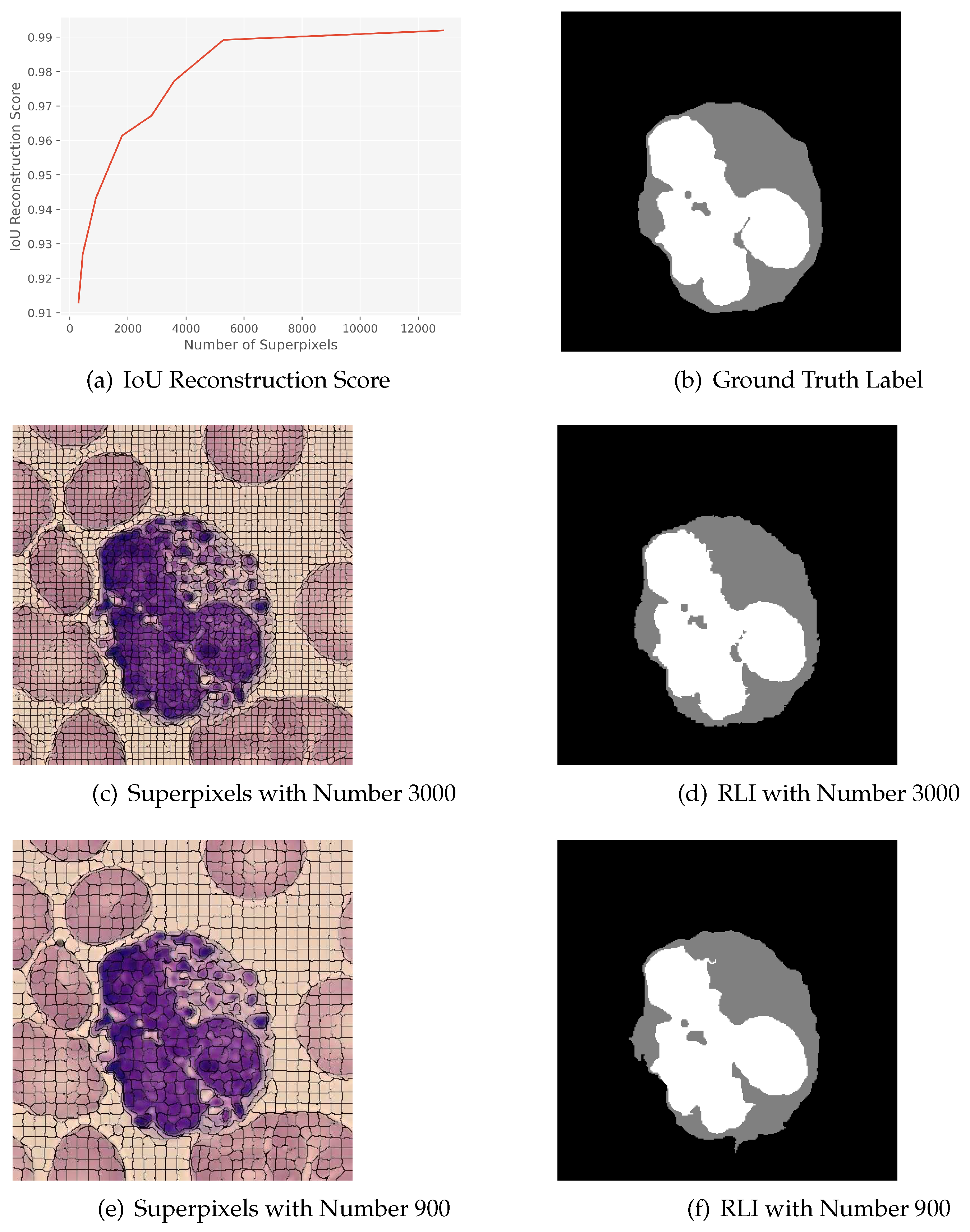
The superpixel quality, and its potential ramifications on segmentation, is an aspect we delve deeply into. By modulating the number of superpixels, we could ascertain its influence. For instance, the WBCs dataset results (illustrated by the red trajectory in Figure 4) signify that as the granularity of the superpixel method amplifies, there’s a corresponding upswing in the mIoU (mean Intersection over Union) score. Balancing optimal segmentation outcomes with computational practicality, we’ve pegged the mean scale of superpixels (S) at 16 for all ensuing experiments.
3.3. Comparison with Mainstream Deep Learning Segmentation Methods
A particularly intricate aspect of the WBCs dataset segmentation is the differentiation between the cytoplasm and the nuclei. Several images present nuclei that are sub-optimally stained, leading to a coloration reminiscent of the cytoplasm. This color overlap often ensnares traditional CNN-based segmentation models, resulting in predicted segmentations marred by interruptions or holes. Ideally, accurate segmentation demands that the representation of the nucleus be a cohesive, uninterrupted region. Our introduced SMGNN model takes an innovative approach by bolstering the connectivity of adjacent superpixels. Therefore, it is proficient in preserving the integrity of the nucleus region, where the capability is vividly showcased in Figure 5.
Figure 4.
(a) The IoU reconstruction score VS number of superpixels. (b) Ground truth label image. (c)(d)(e)(f) Superpixel images and reconstructed label images (RLIs) of two different superpixel numbers. With an increase in the number of superpixels, the RLI tends to converge towards the ground truth label image. This trend indicates that the boundaries of the superpixels become more consistent with the boundaries of the cells, leading to improved quality of the superpixel segmentation.
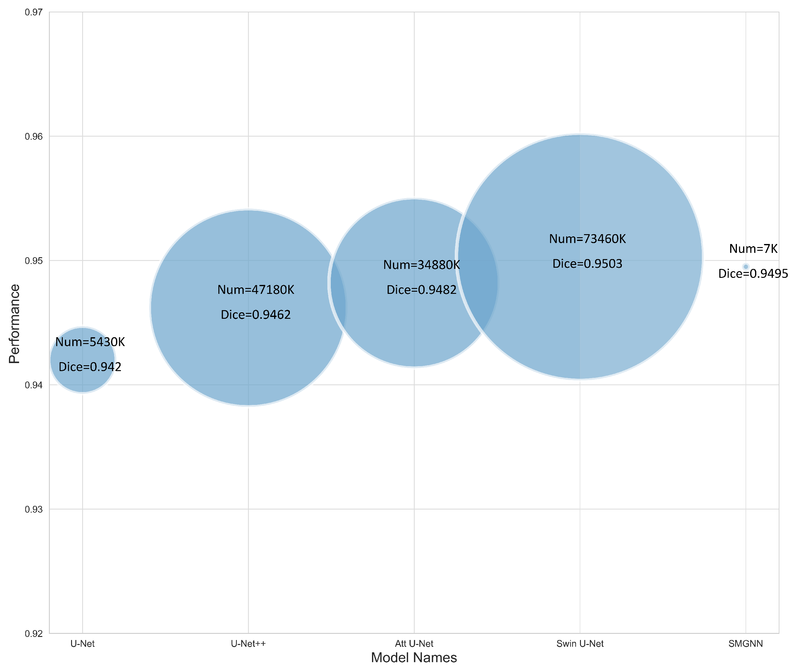
In Figure 6, we show the performance and number of learnable parameters of different deep learning models. Our SMGNN model can reach the SOTA performance while using far fewer parameters.
Figure 5.
The segmentation results on the WBCs dataset. The ground truth (GT) annotation image contains a connected nuclei region without holes inside. Most CNN based methods tend to over-segment the nuclei region induced by the model bias. The SMGNN model can well preserve local connectivity and achieve comparable performance.
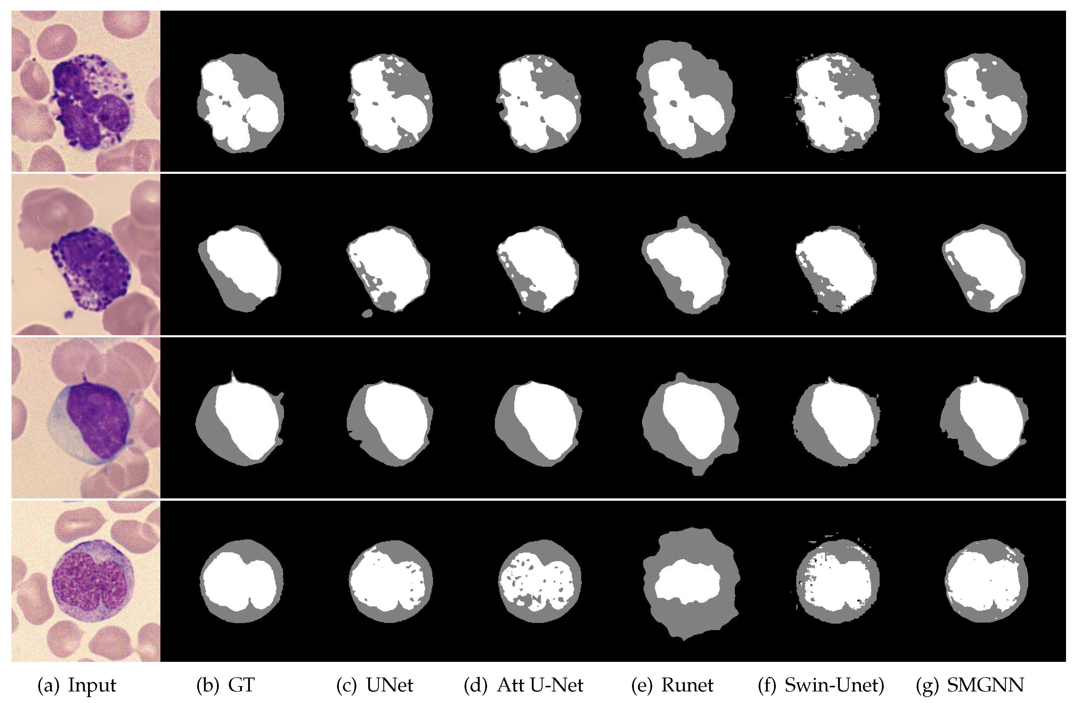
Figure 6.
The comparison of model performance and network parameter size across different models on the WBCs dataset. The center of the circle indicates the Dice score of the model. The radius of the circle indicates the number of learnable parameters. The SMGNN model, utilizing approximately 7000 parameters, achieves comparable performance to models with millions of parameters.
3.4. Ablation Study
To optimize node embeddings within our methodology, we selected the GIN model for the GNN module due to its superior discriminative capacity. Comparative tests with popular GNN models like GCN and GAT revealed that a configuration using three layers of GIN demonstrated an enhanced performance, significantly improving node classification accuracy.
Beyond the conventional setup detailed in Figure 3, which incorporates pixel-level embedding, we ventured into an approach that solely leverages a GNN, transitioning from image-level segmentation components to a strictly node-based classification method, as illustrated in Figure 7. The training for this node classification is driven by a cross-entropy loss function, delineated as follows:
where we use the majority voting rule to define the supepixel label as
guiding the supervised learning in graph space. In Eq. (12), is the round down function, and is the predicted probability of superpixel, and C is the number of semantic classes. Though such a rule may group mistaken pixels whose pixel label is not the majority, the pure GNN methods may achieve good performance when the scale of the superpixel is small. Our ablation studies, as depicted in Figure 8, offer keen insights into the performance nuances of pure GNN-based segmentation models. These models manifest commendable segmentation outcomes when oriented to small-scale superpixel environments. However, as we scale the superpixels, the model’s performance is inversely impacted by its heightened sensitivity to superpixel quality, leading to notable performance drops. Introducing convolutional filters via CNN feature embedding for image-level segmentation does augment the model with additional parameters. Nevertheless, the significance of these filters is evident in the stability they confer upon the model, especially when navigating varying superpixel scales.
This investigation underpins a critical takeaway: the scale of superpixels and a model’s sensitivity to their quality must be harmoniously calibrated. Relying exclusively on GNN-driven segmentation models may prove suboptimal when maneuvering larger superpixel frameworks.
3.5. Effectiveness of Metric Learning on Embedding Space
To understand the impact of metric learning on the embedding space, we visually represent the spatial relationships of superpixels. We assign different colors to these superpixels based on their labels, as determined by Eq. (12). Figure 9, created using UMAP [62], demonstrates the distances among embeddings derived from the GNN. A notable observation from this visualization is the pronounced separation between superpixels with distinct labels—a testament to the efficacy of incorporating metric learning. Furthermore, there’s a heightened cosine similarity between samples that are alike, while distinct samples exhibit reduced similarity. This distinction underscores the model’s ability to effectively differentiate and group superpixels in the embedding space.
3.6. White Blood Cells Type Classification Results
Though the segmentation of cell salient regions, such as the nucleus and cytoplasm, is fundamental and challenging, there are various off-the-shelf methods available for subsequent cell type classification [63,64,65]. Segmentation may provide a direct means to obtain distinguishing characteristics for cell type classification, as cell morphology is closely related to type.
In this research, we employ a light-eight ResNet neural network [66,67] and train a classifier based on the output of segmentation network, as shown in Figure 10. We sample about training images from each classes and leave the remaining for testing. The classification result is shown on Table 1, and our classification method can achieve about overall accuracy. In addition to our proposed segmentation-based cell type recognition system, we also implemented a baseline method to predict cell types without utilizing segmented cell regions. The corresponding results are presented in Table 2, and such method without extraction on slient cell regions can barely achieve overall accuracy. There are also traditional methods employ hand-crafted features extracted from segmented regions, combined with machine learning classifiers like Support Vector Machine (SVM) [63], and such method can get overall accuracy ranging from to . Our proposed deep learning-based automatic recognition system demonstrates high efficiency, and its accuracy can be further improved with an increase in the number of available training samples.
4. Conclusion
In this research paper, we propose a deep learning based automatic recognizing system for the challenging white blood cell image recognizing task. In the first part, our proposed SMGNN segmentation model, which combines superpixel methods and a lightweight Graph Isomorphism Network to significantly reduce memory usage while preserving segmentation capabilities. We innovatively propose superpixel metric learning to capture cross-image global context information, making it highly suitable for medical images with limited training samples. Comparing our model to other mainstream deep learning models, we achieve comparable segmentation performance with a remarkable reduction of at most 10000 times fewer parameters. Through extended numerical experiments, we further investigate the effectiveness of metric learning and the quality of superpixels In the second part, the segmentation-based cell type classification processes exhibit satisfactory results, indicating that the overall automatic recognition algorithms are accurate and efficient for execution in hematological laboratories. We have made our code publicly available at https://github.com/jyh6681/SPXL-GNN, and we encourage its widespread implementation in portable devices of hematologists and remote rural areas.
References
- Mohamed, H.; Omar, R.; Saeed, N.; Essam, A.; Ayman, N.; Mohiy, T.; AbdelRaouf, A. Automated detection of white blood cells cancer diseases. 2018 First international workshop on deep and representation learning (IWDRL). IEEE, 2018, pp. 48–54.
- Kruskall, M.S.; Lee, T.H.; Assmann, S.F.; Laycock, M.; Kalish, L.A.; Lederman, M.M.; Busch, M.P. Survival of transfused donor white blood cells in HIV-infected recipients. Blood, The Journal of the American Society of Hematology 2001, 98, 272–279. [Google Scholar] [CrossRef] [PubMed]
- Xing, F.; Yang, L. Robust nucleus/cell detection and segmentation in digital pathology and microscopy images: a comprehensive review. IEEE reviews in biomedical engineering 2016, 9, 234–263. [Google Scholar] [CrossRef] [PubMed]
- Zheng, X.; Wang, Y.; Wang, G.; Liu, J. Fast and robust segmentation of white blood cell images by self-supervised learning. Micron 2018, 107, 55–71. [Google Scholar] [CrossRef] [PubMed]
- Zhou, Y.; Wu, Y.; Wang, Z.; Wei, B.; Lai, M.; Shou, J.; Fan, Y.; Xu, Y. Cyclic Learning: Bridging Image-level Labels and Nuclei Instance Segmentation. IEEE Transactions on Medical Imaging 2023. [Google Scholar] [CrossRef] [PubMed]
- Gao, Z.; Shi, J.; Zhang, X.; Li, Y.; Zhang, H.; Wu, J.; Wang, C.; Meng, D.; Li, C. Nuclei grading of clear cell renal cell carcinoma in histopathological image by composite high-resolution network. Medical Image Computing and Computer Assisted Intervention–MICCAI 2021: 24th International Conference, Strasbourg, France, September 27–October 1, 2021, Proceedings, Part VIII 24. Springer, 2021, pp. 132–142.
- Ronneberger, O.; Fischer, P.; Brox, T. U-net: Convolutional networks for biomedical image segmentation. International Conference on Medical image computing and computer-assisted intervention. Springer, 2015, pp. 234–241.
- Zhou, Z.; Rahman Siddiquee, M.M.; Tajbakhsh, N.; Liang, J. Unet++: A nested u-net architecture for medical image segmentation. In Deep learning in medical image analysis and multimodal learning for clinical decision support; Springer, 2018; pp. 3–11.
- Huang, H.; Lin, L.; Tong, R.; Hu, H.; Zhang, Q.; Iwamoto, Y.; Han, X.; Chen, Y.W.; Wu, J. Unet 3+: A full-scale connected unet for medical image segmentation. ICASSP 2020-2020 IEEE International Conference on Acoustics, Speech and Signal Processing (ICASSP). IEEE, 2020, pp. 1055–1059.
- Jia, F.; Liu, J.; Tai, X.C. A regularized convolutional neural network for semantic image segmentation. Analysis and Applications 2021, 19, 147–165. [Google Scholar] [CrossRef]
- Dosovitskiy, A.; Beyer, L.; Kolesnikov, A.; Weissenborn, D.; Zhai, X.; Unterthiner, T.; Dehghani, M.; Minderer, M.; Heigold, G.; Gelly, S. ; others. An image is worth 16x16 words: Transformers for image recognition at scale. arXiv preprint arXiv:2010.11929, 2020. [Google Scholar]
- Liu, Z.; Lin, Y.; Cao, Y.; Hu, H.; Wei, Y.; Zhang, Z.; Lin, S.; Guo, B. Swin transformer: Hierarchical vision transformer using shifted windows. Proceedings of the IEEE/CVF International Conference on Computer Vision, 2021, pp. 10012–10022.
- Nicolas Carion, Francisco Massa, G. S.N.U.A.K.; Zagoruyko, S. End-to-End Object Detection with Transformers. ECCV 2020, 2020, pp. 213–229.
- Petit, O.; Thome, N.; Rambour, C.; Themyr, L.; Collins, T.; Soler, L. U-net transformer: Self and cross attention for medical image segmentation. International Workshop on Machine Learning in Medical Imaging. Springer, 2021, pp. 267–276.
- Valanarasu, J.M.J.; Oza, P.; Hacihaliloglu, I.; Patel, V.M. Medical transformer: Gated axial-attention for medical image segmentation. Medical Image Computing and Computer Assisted Intervention–MICCAI 2021: 24th International Conference, Strasbourg, France, September 27–October 1, 2021, Proceedings, Part I 24. Springer, 2021, pp. 36–46.
- Cao, H.; Wang, Y.; Chen, J.; Jiang, D.; Zhang, X.; Tian, Q.; Wang, M. Swin-unet: Unet-like pure transformer for medical image segmentation. Computer Vision–ECCV 2022 Workshops: Tel Aviv, Israel, October 23–27, 2022, Proceedings, Part III. Springer, 2023, pp. 205–218.
- Chi, Z.; Wang, Z.; Yang, M.; Li, D.; Du, W. Learning to capture the query distribution for few-shot learning. IEEE Transactions on Circuits and Systems for Video Technology 2021, 32, 4163–4173. [Google Scholar] [CrossRef]
- Li, G.D.; Masuda, S.; Yamaguchi, D.; Nagai, M. The optimal GNN-PID control system using particle swarm optimization algorithm. International Journal of Innovative Computing, Information and Control 2009, 5, 3457–3469. [Google Scholar]
- Wang, Y.; Yi, K.; Liu, X.; Wang, Y.G.; Jin, S. ACMP: Allen-cahn message passing with attractive and repulsive forces for graph neural networks. The Eleventh International Conference on Learning Representations, 2022.
- Min, S.; Gao, Z.; Peng, J.; Wang, L.; Qin, K.; Fang, B. STGSN—A Spatial–Temporal Graph Neural Network framework for time-evolving social networks. Knowledge-Based Systems 2021, 214, 106746. [Google Scholar] [CrossRef]
- Bumgardner, B.; Tanvir, F.; Saifuddin, K.M.; Akbas, E. Drug-Drug Interaction Prediction: a Purely SMILES Based Approach. 2021 IEEE International Conference on Big Data (Big Data). IEEE, 2021, pp. 5571–5579.
- Bruna, J.; Zaremba, W.; Szlam, A.; LeCun, Y. Spectral networks and locally connected networks on graphs. arXiv preprint arXiv:1312.6203, 2013. [Google Scholar]
- Defferrard, M.; Bresson, X.; Vandergheynst, P. Convolutional neural networks on graphs with fast localized spectral filtering. Advances in neural information processing systems 2016, 29. [Google Scholar]
- Kipf, T.N.; Welling, M. Semi-supervised classification with graph convolutional networks. arXiv preprint arXiv:1609.02907, 2016. [Google Scholar]
- Veličković, P.; Cucurull, G.; Casanova, A.; Romero, A.; Liò, P.; Bengio, Y. Graph Attention Networks. International Conference on Learning Representations, 2018.
- Xu, K.; Hu, W.; Leskovec, J.; Jegelka, S. How powerful are graph neural networks? arXiv preprint arXiv:1810.00826, 2018. [Google Scholar]
- Lu, Y.; Chen, Y.; Zhao, D.; Chen, J. Graph-FCN for Image Semantic Segmentation; Advances in Neural Networks – ISNN 2019, 2019.
- Zhang, L.; Li, X.; Arnab, A.; Yang, K.; Tong, Y.; Torr, P.H. Dual graph convolutional network for semantic segmentation. arXiv preprint arXiv:1909.06121, 2019. [Google Scholar]
- Tian, Z.; Liu, L.; Zhang, Z.; Fei, B. Superpixel-based segmentation for 3D prostate MR images. IEEE transactions on medical imaging 2015, 35, 791–801. [Google Scholar] [CrossRef] [PubMed]
- Monti, F.; Boscaini, D.; Masci, J.; Rodola, E.; Svoboda, J.; Bronstein, M.M. Geometric deep learning on graphs and manifolds using mixture model cnns. Proceedings of the IEEE conference on computer vision and pattern recognition, 2017, pp. 5115–5124.
- Gadde, R.; Jampani, V.; Kiefel, M.; Kappler, D.; Gehler, P.V. Superpixel Convolutional Networks using Bilateral Inceptions. Springer, Cham, 2015. [Google Scholar]
- Avelar, P.H.; Tavares, A.R.; da Silveira, T.L.; Jung, C.R.; Lamb, L.C. Superpixel image classification with graph attention networks. 2020 33rd SIBGRAPI Conference on Graphics, Patterns and Images (SIBGRAPI). IEEE, 2020, pp. 203–209.
- Zhao, W.; Jiao, L.; Ma, W.; Zhao, J.; Zhao, J.; Liu, H.; Cao, X.; Yang, S. Superpixel-based multiple local CNN for panchromatic and multispectral image classification. IEEE Transactions on Geoscience and Remote Sensing 2017, 55, 4141–4156. [Google Scholar] [CrossRef]
- Cui, B.; Xie, X.; Ma, X.; Ren, G.; Ma, Y. Superpixel-based extended random walker for hyperspectral image classification. IEEE Transactions on Geoscience and Remote Sensing 2018, 56, 3233–3243. [Google Scholar] [CrossRef]
- Zhang, S.; Li, S.; Fu, W.; Fang, L. Multiscale superpixel-based sparse representation for hyperspectral image classification. Remote Sensing 2017, 9, 139. [Google Scholar] [CrossRef]
- Liu, Q.; Xiao, L.; Yang, J.; Wei, Z. CNN-enhanced graph convolutional network with pixel-and superpixel-level feature fusion for hyperspectral image classification. IEEE Transactions on Geoscience and Remote Sensing 2020, 59, 8657–8671. [Google Scholar] [CrossRef]
- Felzenszwalb, P.F.; Huttenlocher, D.P. Efficient graph-based image segmentation. International journal of computer vision 2004, 59, 167–181. [Google Scholar] [CrossRef]
- Ren, X.; Malik, J. Learning a classification model for segmentation. Computer Vision, IEEE International Conference on. IEEE Computer Society, 2003, Vol. 2, pp. 10–10.
- Liu, M.Y.; Tuzel, O.; Ramalingam, S.; Chellappa, R. Entropy rate superpixel segmentation. CVPR 2011. IEEE, 2011, pp. 2097–2104.
- Achanta, R.; Shaji, A.; Smith, K.; Lucchi, A.; Fua, P.; Süsstrunk, S. SLIC superpixels compared to state-of-the-art superpixel methods. IEEE transactions on pattern analysis and machine intelligence 2012, 34, 2274–2282. [Google Scholar] [CrossRef] [PubMed]
- Li, Z.; Chen, J. Superpixel segmentation using linear spectral clustering. Proceedings of the IEEE conference on computer vision and pattern recognition, 2015, pp. 1356–1363.
- Liu, Y.J.; Yu, C.C.; Yu, M.J.; He, Y. Manifold SLIC: A fast method to compute content-sensitive superpixels. Proceedings of the IEEE conference on computer vision and pattern recognition, 2016, pp. 651–659.
- Achanta, R.; Susstrunk, S. Superpixels and polygons using simple non-iterative clustering. Proceedings of the IEEE conference on computer vision and pattern recognition, 2017, pp. 4651–4660.
- Tu, W.C.; Liu, M.Y.; Jampani, V.; Sun, D.; Chien, S.Y.; Yang, M.H.; Kautz, J. Learning superpixels with segmentation-aware affinity loss. Proceedings of the IEEE Conference on Computer Vision and Pattern Recognition, 2018, pp. 568–576.
- Jampani, V.; Sun, D.; Liu, M.Y.; Yang, M.H.; Kautz, J. Superpixel sampling networks. Proceedings of the European Conference on Computer Vision (ECCV), 2018, pp. 352–368.
- Yang, F.; Sun, Q.; Jin, H.; Zhou, Z. Superpixel segmentation with fully convolutional networks. Proceedings of the IEEE/CVF conference on computer vision and pattern recognition, 2020, pp. 13964–13973.
- Suzuki, T. Superpixel segmentation via convolutional neural networks with regularized information maximization. ICASSP 2020-2020 IEEE International Conference on Acoustics, Speech and Signal Processing (ICASSP). IEEE, 2020, pp. 2573–2577.
- Zhu, L.; She, Q.; Zhang, B.; Lu, Y.; Lu, Z.; Li, D.; Hu, J. Learning the superpixel in a non-iterative and lifelong manner. Proceedings of the IEEE/CVF Conference on Computer Vision and Pattern Recognition, 2021, pp. 1225–1234.
- Saueressig, C.; Berkley, A.; Munbodh, R.; Singh, R. A joint graph and image convolution network for automatic brain Tumor segmentation. International MICCAI Brainlesion Workshop. Springer, 2021, pp. 356–365.
- Kulikov, V.; Lempitsky, V. Instance segmentation of biological images using harmonic embeddings. Proceedings of the IEEE/CVF Conference on Computer Vision and Pattern Recognition, 2020, pp. 3843–3851.
- Kim, J.; Kim, T.; Kim, S.; Yoo, C.D. Edge-labeling graph neural network for few-shot learning. Proceedings of the IEEE/CVF conference on computer vision and pattern recognition, 2019, pp. 11–20.
- Chen, T.; Kornblith, S.; Norouzi, M.; Hinton, G. A simple framework for contrastive learning of visual representations. International conference on machine learning. PMLR, 2020, pp. 1597–1607.
- Chen, X.; Fan, H.; Girshick, R.; He, K. Improved baselines with momentum contrastive learning. arXiv preprint arXiv:2003.04297, 2020. [Google Scholar]
- He, K.; Fan, H.; Wu, Y.; Xie, S.; Girshick, R. Momentum contrast for unsupervised visual representation learning. Proceedings of the IEEE/CVF conference on computer vision and pattern recognition, 2020, pp. 9729–9738.
- Caron, M.; Misra, I.; Mairal, J.; Goyal, P.; Bojanowski, P.; Joulin, A. Unsupervised learning of visual features by contrasting cluster assignments. Advances in neural information processing systems 2020, 33, 9912–9924. [Google Scholar]
- Wang, W.; Zhou, T.; Yu, F.; Dai, J.; Konukoglu, E.; Van Gool, L. Exploring cross-image pixel contrast for semantic segmentation. Proceedings of the IEEE/CVF International Conference on Computer Vision, 2021, pp. 7303–7313.
- Gilmer, J.; Schoenholz, S.S.; Riley, P.F.; Vinyals, O.; Dahl, G.E. Neural message passing for quantum chemistry. ICML, 2017.
- Weisfeiler, B.; Leman, A. A reduction of a graph to a canonical form and an algebra arising during this reduction, Nauchno–Technicheskaja Informatsia, 9 (1968), 12–16.
- Achanta, R.; Susstrunk, S. Superpixels and Polygons using Simple Non-Iterative Clustering. IEEE Conference on Computer Vision and Pattern Recognition (CVPR), 2017.
- Milletari, F.; Navab, N.; Ahmadi, S.A. V-net: Fully convolutional neural networks for volumetric medical image segmentation. 2016 fourth international conference on 3D vision (3DV). IEEE, 2016, pp. 565–571.
- Kingma, D.P.; Ba, J. Adam: A Method for Stochastic Optimization. ICLR (Poster), 2015.
- McInnes, L.; Healy, J.; Melville, J. Umap: Uniform manifold approximation and projection for dimension reduction. arXiv preprint arXiv:1802.03426, 2018. [Google Scholar]
- Acevedo, A.; Merino, A.; Alférez, S.; Molina, Á.; Boldú, L.; Rodellar, J. A dataset of microscopic peripheral blood cell images for development of automatic recognition systems. Data in brief 2020, 30. [Google Scholar] [CrossRef] [PubMed]
- Yampri, P.; Pintavirooj, C.; Daochai, S.; Teartulakarn, S. White blood cell classification based on the combination of eigen cell and parametric feature detection. 2006 1ST IEEE conference on industrial electronics and applications. IEEE, 2006, pp. 1–4.
- Livieris, I.E.; Pintelas, E.; Kanavos, A.; Pintelas, P. Identification of blood cell subtypes from images using an improved SSL algorithm. Biomedical Journal of Scientific & Technical Research 2018, 9, 6923–6929. [Google Scholar]
- Banerjee, R.; Ghose, A. A Light-Weight Deep Residual Network for Classification of Abnormal Heart Rhythms on Tiny Devices. Joint European Conference on Machine Learning and Knowledge Discovery in Databases. Springer, 2022, pp. 317–331.
- He, K.; Zhang, X.; Ren, S.; Sun, J. Deep residual learning for image recognition. Proceedings of the IEEE conference on computer vision and pattern recognition, 2016, pp. 770–778.
| 1 |
Figure 1.
Sample images of five different types of white blood cells. The colors of different images exhibit significant variations, and the boundaries of the cytoplasm are often ambiguous, posing a considerable challenge in accurately recognizing the shape of WBCs.
Figure 1.
Sample images of five different types of white blood cells. The colors of different images exhibit significant variations, and the boundaries of the cytoplasm are often ambiguous, posing a considerable challenge in accurately recognizing the shape of WBCs.
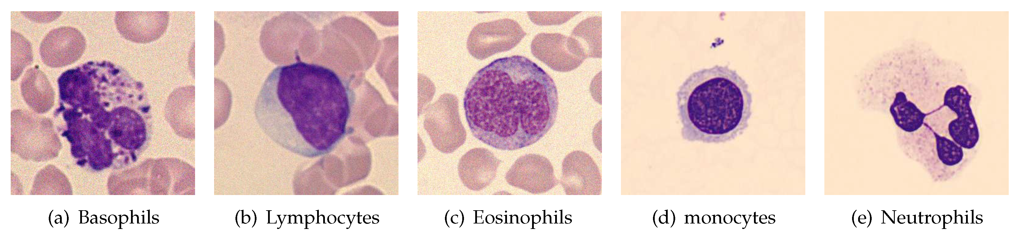
Figure 3.
The framework of our proposed SMGNN for medical image segmentation consists of three main stages: (1) Create Superpixel Graph: The input images are initially over-segmented, generating multiple superpixels. Subsequently, a superpixel graph is constructed based on these segments. (2) Graph Representation Network: The superpixel embeddings are learned using a combination of GNN and metric learning techniques. This stage focuses on capturing the relationships and representations within the superpixel graph. (3) Convert to Image Space Feature: To facilitate segmentation, the superpixel graph is projected back to the image domain using the association matrix. CNN layer is utilized to perform the segmentation task in the image space. The training process is supervised by superpixel metric loss function in the graph space and Dice loss function in the image space.
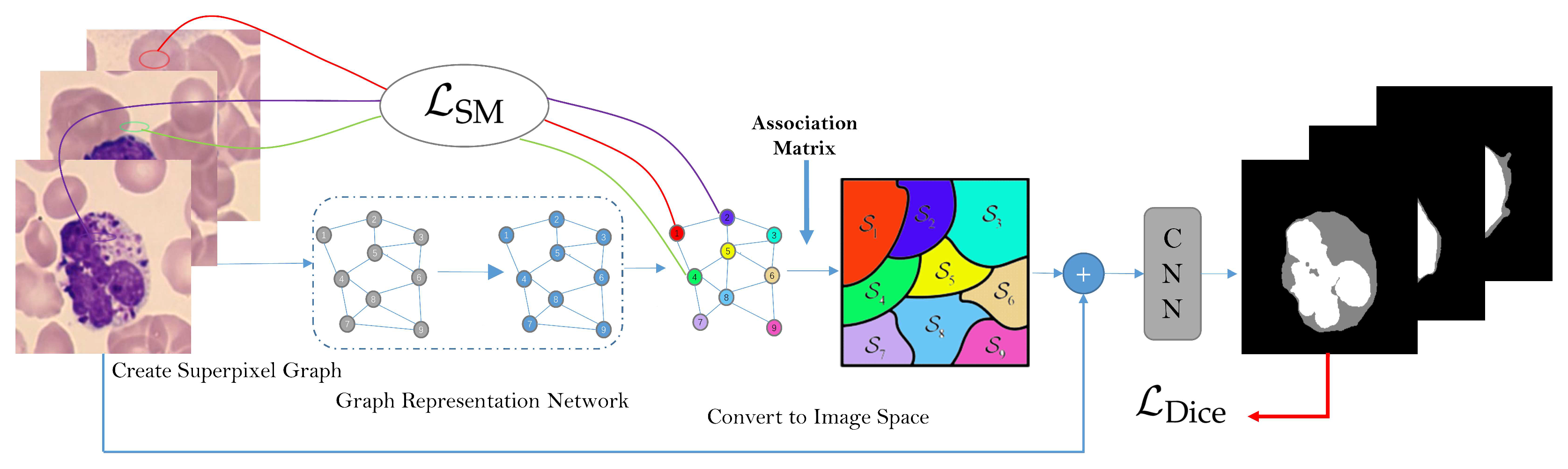
Figure 7.
Pure GNN method converts segmentation task as the superpixel classification task, without involving learning in image space. The classification task is trained with cross entropy loss function . The classified superpixels are projected back to the image domain through an association matrix.
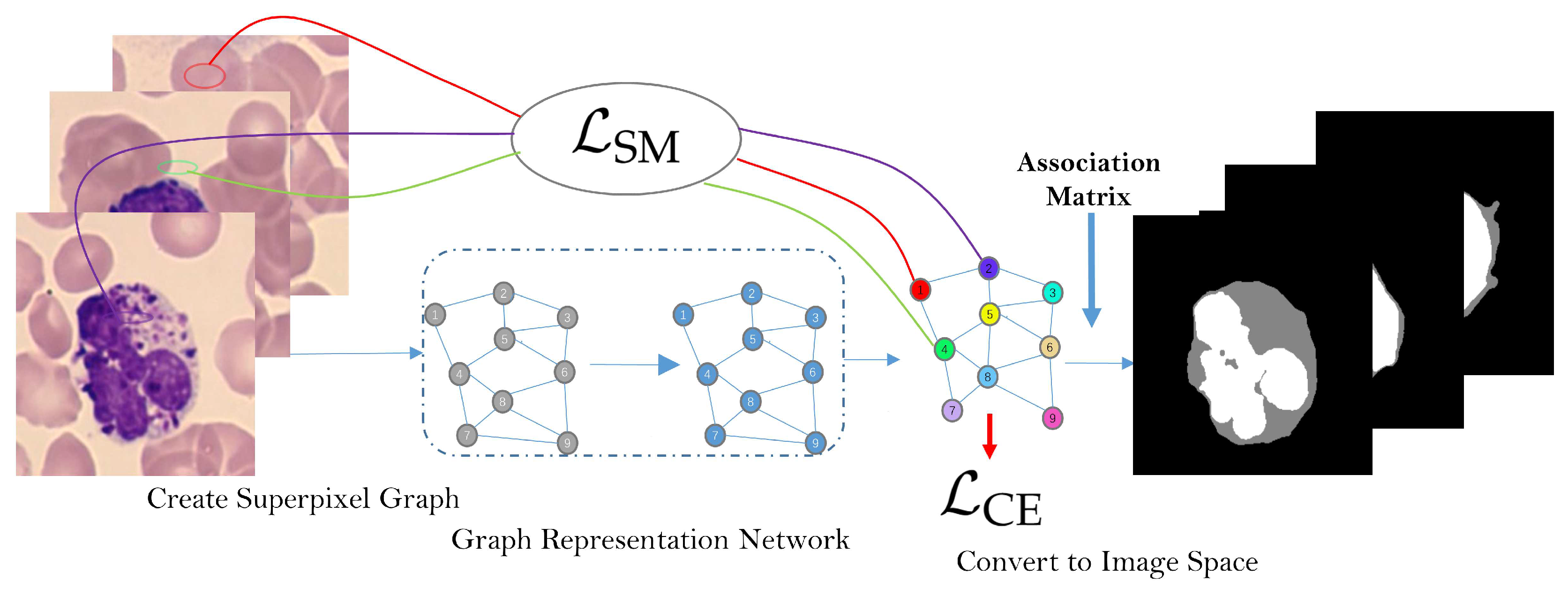
Figure 8.
This ablation study delves into the impact of metric learning and convolutional filtering within the image domain. Segmentation trials were undertaken on WBCs datasets.
Figure 8.
This ablation study delves into the impact of metric learning and convolutional filtering within the image domain. Segmentation trials were undertaken on WBCs datasets.
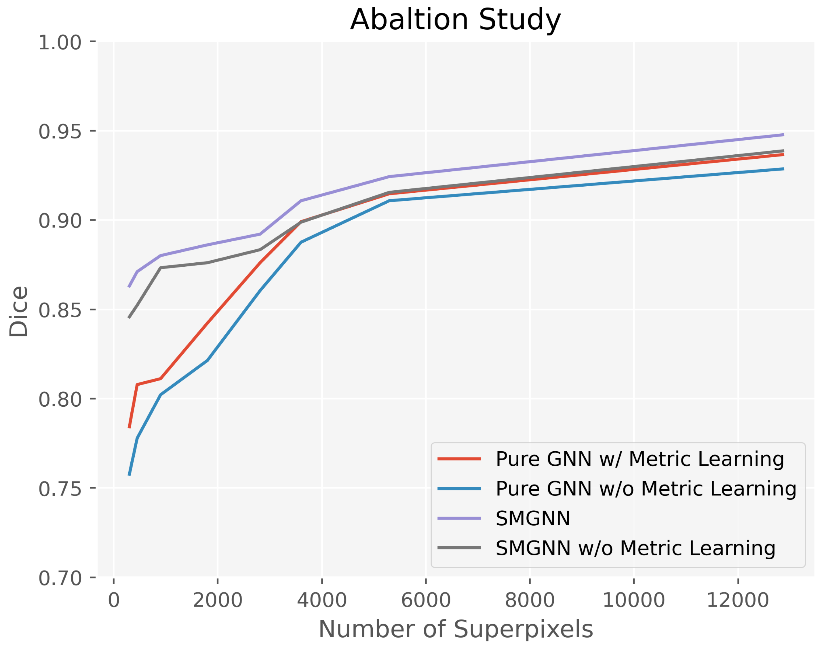
Figure 9.
(a) Without superpixel metric learning, the embeddings are hardly able to separate. (b) With superpixel metric learning, the well learned embeddings will form into three groups corresponding to nuclei, cytoplasm and background.
Figure 9.
(a) Without superpixel metric learning, the embeddings are hardly able to separate. (b) With superpixel metric learning, the well learned embeddings will form into three groups corresponding to nuclei, cytoplasm and background.
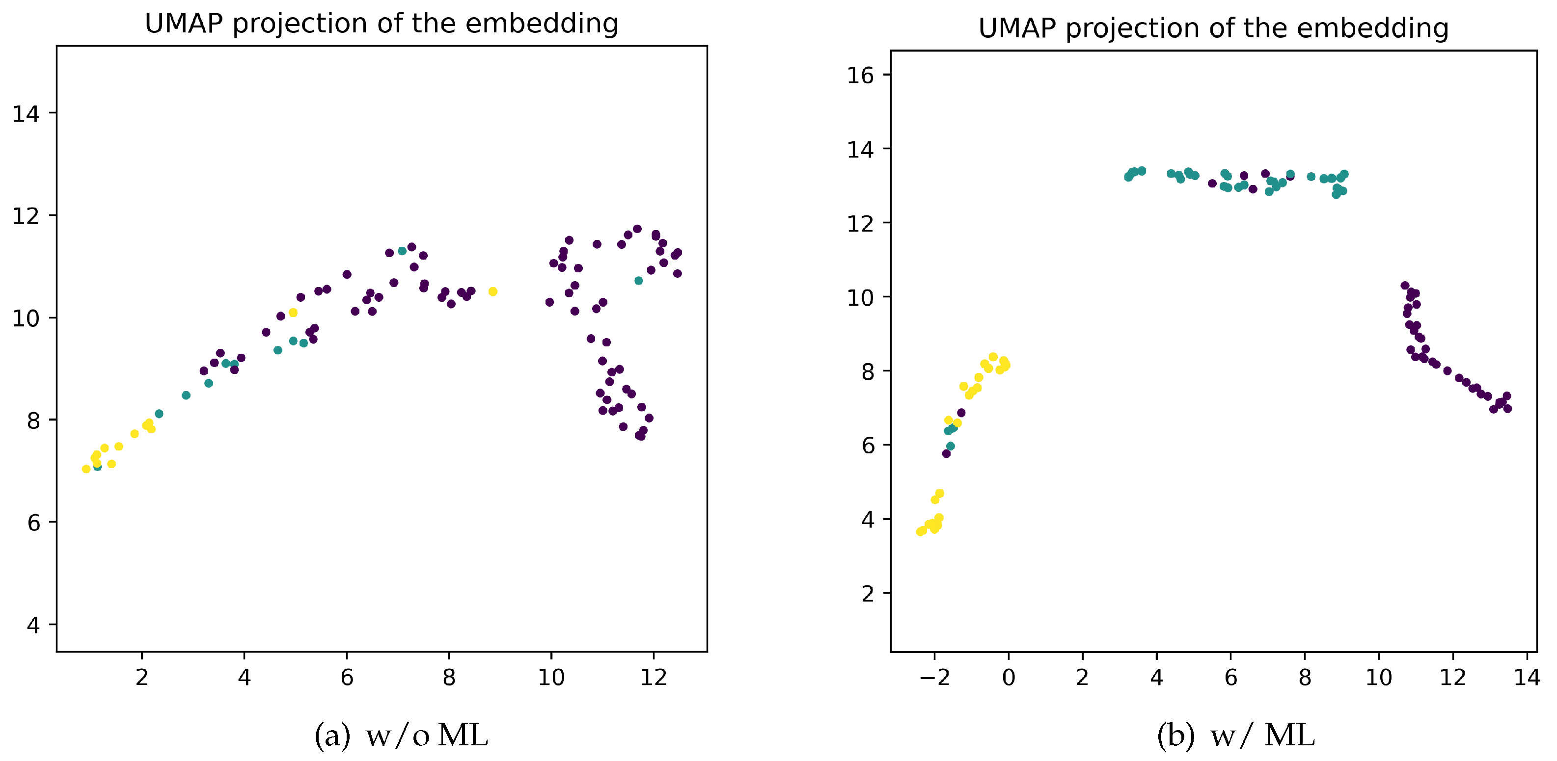
Figure 10.
The segmentation-based cell type classification workflow. The segmented salient region implicitly provides important cell features, such as shape, perimeter, mean and variance of the nucleus boundaries. The light-weight ResNet extract region-level embeddings to classify five cell types.
Figure 10.
The segmentation-based cell type classification workflow. The segmented salient region implicitly provides important cell features, such as shape, perimeter, mean and variance of the nucleus boundaries. The light-weight ResNet extract region-level embeddings to classify five cell types.
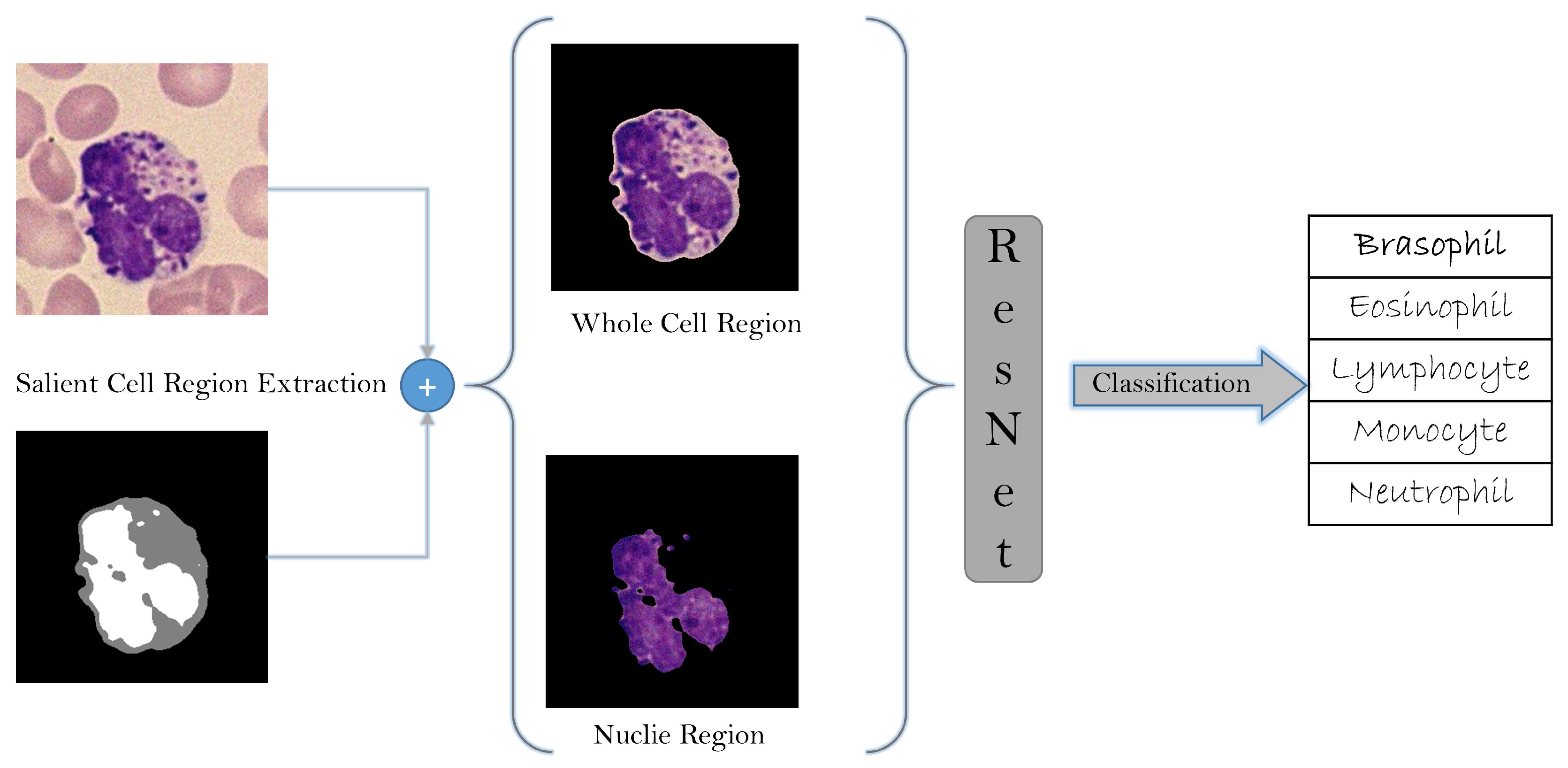

Table 1.
Confusion matrix, Accuracy, and overall accuracy with Resnet classification network using segmenteation results of SMGNN.
Table 1.
Confusion matrix, Accuracy, and overall accuracy with Resnet classification network using segmenteation results of SMGNN.
| Accuracy | ||||||
|---|---|---|---|---|---|---|
| Basophil | 2 | 0 | 0 | 0 | 0 | |
| Eosinophil | 0 | 8 | 0 | 0 | 0 | |
| Lymphocyte | 0 | 0 | 23 | 1 | 0 | |
| Monocyte | 0 | 0 | 0 | 10 | 0 | |
| Neutrophil | 1 | 0 | 0 | 0 | 16 | |
| Overall Accuracy | - | - | - | - | - |
Table 2.
Confusion matrix, Accuracy, and overall accuracy with Resnet classification network without segmenteation methods.
Table 2.
Confusion matrix, Accuracy, and overall accuracy with Resnet classification network without segmenteation methods.
| Accuracy | ||||||
|---|---|---|---|---|---|---|
| Basophil | 1 | 1 | 0 | 0 | 0 | |
| Eosinophil | 2 | 5 | 0 | 0 | 1 | |
| Lymphocyte | 0 | 1 | 20 | 2 | 1 | |
| Monocyte | 0 | 0 | 3 | 6 | 1 | |
| Neutrophil | 2 | 1 | 2 | 0 | 12 | |
| Overall Accuracy | - | - | - | - | - |
Disclaimer/Publisher’s Note: The statements, opinions and data contained in all publications are solely those of the individual author(s) and contributor(s) and not of MDPI and/or the editor(s). MDPI and/or the editor(s) disclaim responsibility for any injury to people or property resulting from any ideas, methods, instructions or products referred to in the content. |
© 2023 by the authors. Licensee MDPI, Basel, Switzerland. This article is an open access article distributed under the terms and conditions of the Creative Commons Attribution (CC BY) license (http://creativecommons.org/licenses/by/4.0/).
Copyright: This open access article is published under a Creative Commons CC BY 4.0 license, which permit the free download, distribution, and reuse, provided that the author and preprint are cited in any reuse.


