Submitted:
25 August 2023
Posted:
29 August 2023
You are already at the latest version
Abstract
The average sizes \ {\bar{L}}_{i\ } and their dispersion W_i along the i-th axis of crystallites in powders are used to determine the X-ray diffraction sizes, D_{i\ XRD}, averaged over crystallite columns within the BWA method. Numerical calculations have been carried out for an orthorhombic lattice of crystallites, such as LiFePO4, NMC, having Lamé's g-type superellipsoid shape. For Lognormal distributions, the analytical expression for the normalized coefficient Kn is found and includes two constants. The first K_{g,0} is a constant at W→0, the second K_g is a constant depending on the g -type shape. The dependences of D_{i\ XRD} are also calculated for Normal distribution. A fairly simple equation can be obtained as a result of analytical transformations in the framework of experimentally validated approximations. However, a simpler way is to carry out numerical computer calculations with subsequent approximation of the calculated curves. Using the obtained analytical expressions to control technologies from nuclear fuel to cathode materials will improve the efficiency of flexible energy network especially storage in autonomous and standby power plants.
Keywords:
crystallites in powders
; Lamé's shape
; X-ray sizes
; Bertaut-Warren-Averbach
; Normal distributions
; Lognormal distribution
; energy storage
; energy optimization
1. Introduction
P. Scherrer began studying the shape of X-ray lines (LPA - line-profile analysis) to determine the sizes of nanometer objects in 1918. The history is described in [1, 2], and the latest results in [3]. In 1950, Bertaut [4] and Warren, Averbach [5] showed that the total diffraction intensity is the sum of individual diffractions from columns perpendicular to the planes that make up the crystallite. The magnitude of the size-induced broadening of diffraction reflections depends not only on the average sizes of crystallites, but also on the statistics of their distributions. The situation is described in detail in [4-9] and the following equation is assumed to hold
Thus, the task of using the BWA method is reduced to determining the normalized coefficient by integrating (1) and summing over all crystallites, taking into account their shape, as well as the statistics of their distributions.
Based on TEM and SEM studies [2, 7, 10, 11], various size distribution functions: Lognormal, Normal, Gamma, and Poisson are normally used, more precisely, their one-dimensional projections onto some linear dimension. The first two of them can be used in their 3-dimensional versions with pairwise correlations between sizes along the coordinate axes [12-14], while for the last two such a possibility is not “transparent and easily accessible” [15-17]. In some exceptional cases, analytical approximations of distributions with a large dispersion of sizes may be useful [11]. This is probably also due to the fact that in some ranges of dispersion and average sizes, the Lognormal distribution is visually close, for example, to the Gamma distribution (see SI).
Currently, a large number of programs for processing diffractograms and determining have been developed. First of all, it is necessary to take into account the instrumental contribution to diffraction line width [18, 19], and then the general microstructure refinement of all peak profiles (WPPM – Whole Powder Pattern Modeling) procedure can be used [3, 10, 11]. The size–strain line broadening analysis can be combined with evaluating the crystallographic texture of various nanosized powders [20,21,22] in the Rietveld refinement software known as Material Analysis Using Diffraction (MAUD) [23]. In TOPAS (Bruker) software anisotropic crystallite size analysis is also implemented. The accuracy of the double-Voigt approach and the dimensional parameters obtained for triaxial ellipsoid, elliptic cylinder and cuboid is discussed in [24, 25].
Thus, there is a fairly reliable procedure for determining the X-ray diffraction sizes of anisotropic powders, in which their size distribution is assumed to be known a priori, or by inspecting histograms obtained by counting a small number of particles. In the absence of more complete information about the 3-dimensionality of these distributions, the use of the BWA method in the form of equation (1) loses its meaning due to a large error. The known value of the coefficient can reduce the error that is very useful for more precise control of technology and predicting the target parameters of powders.
In this work, this problem is solved by the following numerical calculations: 1) the histograms of particle size distributions are simulated using 3D Lognormal or Normal functions in the form of a 3-dimensional and N-bit matrix, 2) the matrix of averaged columns of crystallites is calculated with the shape of g-type superellipsoids and the sizes corresponding to the histogram bins, 3) the value of , defined as the average column length of the whole powder sample along the i-th axis, is calculated by element-by-element multiplication of these two matrices and then summing the matrix elements along the i-th axis.
2. Calculation model
2.1. Shape of crystallites
Lamé's surface of g-type superellipsoids is described by the implicit equation
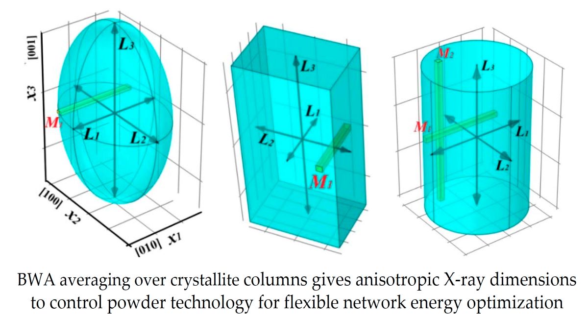
Figure 1 shows anisotropic crystallites and columns along the 1st crystallographic direction. These forms are also used in the TOPAS Rietveld refinement [25]. Replacing x1 in (2) with , we obtain for the length
For we get
The double integration in (5) is carried out over the integration region Reg of the central section of the ellipsoid perpendicular to the 1st axis,
The advantage of using Lamé's superellipsoids is the ability to determine their volume and cross-sectional area perpendicular to column M1 [26, 29], respectively, by using beta functions
In particular, knowing the mass of the cathode powder, its density and the statistics of the size distribution of crystallites, with the equations (7, 8) it is possible to determine the inner surface of the cathode and use it to improve the accuracy of determining the diffusion coefficient using the Randles-Sevcik equation [14], as well as for quantitative calculations of the rate of electrochemical reactions using the Butler–Volmer equation [27]. In this case, the shape of crystallites must be preliminarily determined by analyzing TEM and SEM images of crystallites either visually or using software processing methods [29-32].
2.2. Crystallite statistics
In the study of the structural and electrochemical properties of LiFePO4 powders, Lognormal [33,34,35,36,37,38,39], Normal [40,41,42], and Weibull [36, 37] distributions were observed earlier. The latter was also used to describe carbon conglomerates of anode electrodes [39, 43]. Gamma and Lognormal distributions, as noted above [10, 11], were used in the analysis of specially tested CeO2 powders. There are the following structural and technological justifications for their use:
- In [44], it was shown that during the crushing of rocks, a Lognormal distribution of products occurs, which is due to the multifactorial character of the crushing process itself;
- In [45], the Normal distribution arises as a result of aggregative growth and oriented attachment of nanocrystals;
- In [43], the Weibull distribution results from the restructuring of the electrode morphology during battery usage;
In the SI section, these 4 functions are used to construct the one-dimensional histograms of size (diameter) distributions for 8000 virtual spherical particles. They can be used at the first stage of visual selection of the experimental distribution type.
It was noted above that only the Lognormal [13,14] and Normal [12] distributions can be used to describe anisotropic particles, taking into account their pairwise covariances between the sizes. For the remaining two, they can also be adjusted to Lognormal and Normal with smaller errors compared to those arising when covariances are not taken into account.
In [49], marginal size distributions of crystallites in LiFePO4 powders were determined along all three crystallographic axes, and in [14] the parameters of the 3-dimensional lognormal function were determined
Below we also use the Normal distribution in the form [15]
The most significant difference between (10) and (9) is the linear scale used in (10), and the dimension of the dispersion: in (9) the dispersion W is dimensionless, and in (10) it has the dimension of length. In the calculations, it will be normalized to the average length along the i-th direction, which makes the calculations more general.
2.3. X-ray size calculation
According to (1), the X-ray diffraction size along the 1st axis is the average of the lengths of the columns , shown in Figure 1, over all powder crystallites. We obtain it by averaging over the i-th crystallite using integration (5) over the cross section (6) followed by averaging over all N powder crystallites using function (9) or (10). To do this, we use the Mathematica 12 software for element-by-element matrix multiplication and their summation in the following form, for example, for the Lognormal distribution
Thus, the task of numerical calculations (11) is to determine the dependence of the coefficient in (5) on g – the type of superellipsoids and on the following parameters of the Lognormal (9) or Normal (10) distributions: – average sizes, Wi – dispersion, and – correlation coefficients of the matrix .
3. Results of calculations and their discussion
In the presence of a large number of parameters, it is necessary to establish their hierarchy, evaluate their possible ranges, and also determine the number of bins (discreteness or dimension) of the histograms [50, 51], which is equal to the matrix dimensions used in (11) in our case. It has been verified that the bin number should be at least 15-20 for a small discretization error, comparable to the errors of powder structural studies (see SI).
3.1. Lognormal distribution
Parameter ranges. For high quality LiFePO4 powders, the parameters of the function fall in the following ranges: 40÷500 nm, ~ 0.3÷0.6, r12,13,23 ~ 0.4÷0.7 [27].
To explain the calculation algorithm, the test results for 8000 crystallites and a 20-bin distribution histogram by analogy with [27, 49] are shown in Figure 2. SI contains similar figures and numerical values of 6-bit matrices, which were used to check and control the stages of calculations and to determine the discretization error. From Figure 2b it can be seen that the histogram of X-ray diffraction size distribution shifts to the region of large sizes. This usually occurs with an increase in the dimensionality of the averages: from 1D to 3D. The linear dependence of on L1 exactly corresponds to the value of Kn = ¾ (¾ of ) in (5), Figure 2a (right scale). The sum of 270.41 nm is much larger than 240 nm, that suggests Kn > ¾, which is larger than expected for ellipsoidal crystallites with a small dispersion value W.
Dependences of Kn on correlation coefficients. The calculations illustrated in Figure 2 ignore the dependence of Kn on the correlation coefficients and on their anisotropy. Figure 3 shows the results of testing these assumptions and draws the following conclusions:
- 1. After normalization , the coefficients Kn do not depend on the values of the average sizes in the tested range from 80 to 600 nm, i.e. the normalization significantly expands the universality of the developed calculation procedure.
- 2. A weak dependence of Kn on r is observed at r < 0.7, i.e. in the range of values observed in high quality LiFePO4 samples. However, as shown in [27], this dependence is quite significant for the values of their electrochemical capacitances. Therefore, here and below the calculations are performed for the value r12 = r13 = r23 = r = 0.5.
- 3. The observed dependence at r > 0.7 is related to the histogram discreteness. Only in this region anisotropy of crystallite sizes along other crystallographic directions can affect the calculation results. It also expands the universality of the developed calculation procedure.
Dependencies of Kn on the dispersion W1. Figure 4 shows the results of calculations that can already be directly used in the development of technology for electrode crystalline powders with a higher accuracy in determining their structural parameters compared to those previously used in [14, 27] to determine the block structure of crystallites [49], to assess the potential of the developed technologies, and to optimize it [14]. From Figure 4, the following conclusions can be drawn:
- 1. For the Lognormal crystallite size distribution the following analytical expression for Kn is foundwhere Kg,0 is a constant at W→0, Kg is a constant depending on the g-type shape. The values of these constants are collected in Table 1.Kn =( Kg,0 + Kg W2 )
- 2. Equation (12) is valid up to the values of W1 ~ 0.6. For larger values, it is necessary to increase the bit length of the histograms, which is possible with a 2÷3-fold increase in the number of measured particles. On the other hand, the error of using 6-bit histograms with 2÷3 times smaller number of particles (up to 1000÷2000) will be no more than 1%.
3.2. Normal distribution
Parameter ranges. The examples of 20-bit histograms for 8000 particles given in SI show their main feature: at W > 1, the proportion of small-sized particles increases due to the impossibility of negative values of the particle size, and at W < 1, it is located entirely on the positive part of the abscissa axis. Thus, the average dimensions of ~ 40–500 nm and the value of the normalized dispersion covering the point W=1 were used in the calculations.
Dependences of Kn on the correlation coefficients. Based on Figure 5, the following conclusions are made:
- At small W < 0.5-0.8, there is no dependence of Kn on r and W, as well as no dependence of the calculated values on the values of the distribution parameters along the 2nd 3rd axes, as is observed in Figure 3 for the values of r > 0.7 of Lognormal distributions. The values of Kn calculated at small W, up to nearly 1, can be considered universal constants equal to Kg,0 with a small error (Table 1).
- For large W up to 2, the dependences along the 2nd and 3rd axes are significantly weak. In particular, as can be seen from Figure 5 for the curves with W=2, the 30% changes in the values of dispersion lead to much smaller changes of less than 3% in Kn.
Thus, the calculations with equal parameters along all three axes can be considered accurate. With anisotropic deviations of up to 30% in the distribution parameters at large W, the error of 3% can occur.
Dependences of Kn on dispersion W1. Figure 6 shows the results of calculations that can also be directly used in the development of technology for electrode crystalline powders with Normally distributed crystallite sizes to determine block structure [49], assess the potential of the developed technologies, and optimize it [14].
As can be seen from Figure 6, the solid lines for W1=W2 =W3 can be approximated by two straight lines in the region W1 < 2.4 that intersect at the point W = 1. Analytically, the situation can be described by the so-called piecewise-continuous function [52]
Obviously, the rather simple equations (12, 13) can be obtained as a result of analytical transformations within the framework of the corresponding approximations. However, a simpler way was to carry out numerical calculations with subsequent approximation of the calculated curves.
4. Conclusions
The use of the BWA (Bertaut-Warren-Averbach) method is an important tool for studying the structure of crystalline powders, namely, for relating the anisotropic X-ray diffraction sizes of crystallites to their anisotropic linear sizes (1). First, the lengths of the columns are averaged over the volume of a typical crystallite. Here the anisotropic shape of the crystallite is important. Second, the lengths of the columns are averaged over all crystallites of the powder under study. Here, the distribution of crystallites over their anisotropic linear dimensions is important. A sign of these averaging is the presence of a relation for the dimensions (length)4/(length)3. In particular, therefore, the result of averaging over a crystallite is divided by the volume of this crystallite. Using these principles of the BWA method, the following results were obtained:
- Numerical calculations have been carried out for the crystallites with orthorhombic lattice, such as LiFePO4, NMC. The shape of crystallites was approximated with the Lamé's g-type superellipsoids including cuboids at large g > 20÷30. The values of the dimensional parameters of the powders were close to the ones observed experimentally.
- In the presence of anisotropy, the equations (12, 13) can be normalized to the length of the crystallite along its i-th axis; the normalized (dimensionless) distribution dispersions can also be used for Lognormal and Normal distributions. The universality of the calculation results is limited by the discreteness of the matrices, which is due to the discreteness of the experimental histograms of crystallite sizes in the powders under study.
- For Lognormal distributions, the coefficient Kn depend weakly on the correlation parameter r for r < 0.7, i.e. in the range of values observed in high quality LiFePO4 samples. The observed dependence at r > 0.7 is related to the discreteness of the histograms and to the effect of crystallite size anisotropy along other crystallographic directions.
- For the Lognormal size distribution of crystallites, the following universal analytical expression for Kn (12) is found, which is applicable up to values of W1 ~ 0.6. For larger values, it is necessary to increase the bit number of the histograms, which requires a 2-3-times increase in the number of measured particles.
- For Normal distributions with small W < 0.5-0.7, there is no dependence of Kn on r and W, and the calculated values are independent of the values of the distribution parameters along the 2nd 3rd axes. The calculated Kn for small W ≤ 1, can be considered as universal constants.
- For Normal distributions at large W ≤ 2, the dependences of Kn on the parameters of other axes are significantly weak, in particular, for the curves with W1 = 2, 30% changes in dispersions along the 2nd and 3rd axes lead to much smaller changes in Kn of no more than 3%.
- For Normal distributions, the dependences of Kn on W for the ratios W1=W2 =W3 can be approximated by two straight lines that intersect at the point of W = 1. Analytically, the situation can be described by the so-called piecewise-continuous function (13).
- For Gamma and Poisson distributions the mathematically reliable ways to describe correlations between sizes along different coordinate axes are lacking. In some cases, these distributions are visually close to the Lognormal and Normal functions which can be used instead of Gamma and Poisson.
- An elliptical cylinder (bar) (shown in Figure 1с) can be described as a combination of an ellipsoid with M1 columns along the x1 axis and a cuboid with M2 columns along x3.
- The use of the BWA method is carried out on the example of LiFePO4 and is justified by the fact that this compound has been studied quite well, so the development stages and final conclusions can be varied. In the other case of crystalline powders with a non-orthorhombic lattice, it is necessary to take into account the angles between the axes [9]. In this case, it becomes possible to widely use the BWA method for studying various crystalline powders: other electrode and atmospheric contaminants [47], as well as nuclear fuel and materials [53,54].
Supplementary Materials
The following supporting information can be downloaded at the website of this paper posted on Preprints.org. Figure S1 about Lognormal, Normal, Gamma and Weibull distributions, Figure S2, S3 about checking and controlling the stages of numerical calculations, Figure S4 about the dependence on the number of digits N of the column length, Figure S5 about comparing curves with 20 and 30 histogram sizes.
Author Contributions
B.A, conceptualization, writing, modeling; K.O., data analysis, validation; M.F, software, calculations; K.I., XRD conceptualization, data curation. .
Funding
This research received no external funding.
Data Availability Statement
Not applicable.
Conflicts of Interest
The authors declare no conflict of interest.
References
- Langford, J. I.; Wilson, A. J. C. Sheerer after Sixty Years: A Survey and Some New Results in the Determination of Crystallite Size. Appl. Crist. 1978, 11, 102-113. [CrossRef]
- Langford, J. I. Line Profile Analysis: A Historical Overview. Diffraction Analysis of the Microstructure of Materials. Ch.1. pp. 3–13. Editors Mittemeijer, E.J.; Scardi, P. Series Title Springer Series in Materials Science Springer Berlin, Heidelberg 2004; pp. 1–557. [CrossRef]
- Leoni, M. Domain size and domain-size distributions. International Tables for Crystallography 2019, H, 524–537. doi:10.1107/97809553602060000966.
- Bertaut, E.F. Raies de Debye-Scherrer et R Spartition des Dimensions des Domaines de Bragg dans les Poudres Polycristallines. Acta Cryst. 1950, 3, 14–18. [CrossRef]
- Warren, B.E.; Averbach, B.L. The Effect of Cold Work Distortion on XRay Patterns. J. Appl. Phys. 1950, 21, 595–599. doi: 10.1063/1.1699713.
- Guinier, A. X-Ray Diffraction in Crystals, Imperfect Crystals and Amorphous Bodies, Freeman, San Francisco, 1963; pp. 1–379.
- Matyi, R.J.; Schwartz, L.H.; Butt, J.B. Particle size, particle size distribution, and related measurements of supported metal catalysts. Catalysis Reviews Science and Engineering 1987, 29, 41–99. [CrossRef]
- Krill, C.E.; Birringer, R. Estimating grain-size distributions in nanocrystalline materials from X-ray diffraction profile analysis. Philosophical Magazine 1998, A 77, 621–640. dx.doi.org/10.1080/01418619808224072.
- Žunić, T.B.; Dohrup, J. Use of an ellipsoid model for the determination of average crystallite shape and size in polycrystalline samples. Powder Diffr. 1999, 14(3), 203–207. [CrossRef]
- Scardi, P.; Leoni, M. Whole Powder Pattern Modelling: Theory and Applications. Diffraction Analysis of the Microstructure of Materials. Ch.3. p.51-91. there in [2].
- Popa, N.C.; Balzar, D. An analytical approximation for a size-broadened profile given by the lognormal and gamma distributions. J. Appl. Cryst. 2002, 35, 338–346. [CrossRef]
- Prince, S. J. D. Computer Vision: Models, Learning, and Inference (Instructor's Solution Manual). Cambridge University Press. 2012; pp. 1–151. www.cse.psu.edu/~rtc12/CSE586/lectures/06_Learning_And_Inference_BobEdits.pdf.
- Tarmast, G. Multivariate log – Normal distribution, 53rd ISI World Statistics Congress, Seoul, 2001, https://2001.isiproceedings.org/.
- Bobyl, A.; Nam, S.-С.; Song, J.-H.; Ivanishchev, A.; Ushakov, A. Rate Capability of LiFePO4 Cathodes and the Shape Engineering of Their Anisotropic Crystallites. J. Electrochem. Sci. Technol. 2022, 13, 438–452. [CrossRef]
- Kotz, S; Balakrishnan, N.; N.L. Johnson, N.L. Continuous multivariate distributions. Wiley series in probability and statistics 2000, 1, Ch.46, 251–348. doi:10.1002/0471722065.
- Karlis, D.; Xekalaki, E. Mixed Poisson Distributions. International Statistical Review 2005, 73(1), 35–58. [CrossRef]
- Bladt, M.; Nielsen, B.F. An overview of multivariate gamma distributions as seen from a (multivariate) matrix exponential perspective. ACM Sigmetrics Performance Evaluation Review 2012, 39(4), 34. doi:10.1145/2185395.2185425.
- Scardi, P.; Lutterotti, L.; Maistrelli. P. Experimental determination of the instrumental broadening in the Bragg-Brentano geometry. Powder Diffraction 1994, 9 (3), 180–186. [CrossRef]
- Kern, A.; Coelho, A.A.; Cheary, R.W. Convolution Based Profile Fitting. Ch.2 pp.18–50, there in [2].
- Lutterotti, L.; Matthies, S.; Wenk, H.R.; Schultz, A.S.; Richardson, J.W. Combined texture and structure analysis of deformed limestone from time-of-flight neutron diffraction spectra. J Appl. Phys. 1997, 81, 594–600. [CrossRef]
- Balzar, D.; Audebrand, N.; Daymond, M. R.; Fitch, A.; Hewat, A.; Langford, J. I.; Le Bail, A.; Louër, D.; Masson, O.; McCowan, C. N.; Popa, N. C.; Stephens, P. W.; Toby B. H. Size-strain line-broadening analysis of the ceria round-robin sample. J. Appl. Cryst. 2004, 37, 911–924. [CrossRef]
- Popa, N. C. Stress and strain. International Tables for Crystallography 2019, H, 538–554. doi:10.1107/97809553602060000967.
- Saville, A.I.; Creuziger, A.; Mitchell, E.B.; Vogel, S.C.; Benzing, J.T.; Klemm-Toole, J.; Clarke K.D.; Clarke A.J. MAUD Rietveld Refinement Software for Neutron Diffraction Texture Studies of Single- and Dual-Phase Materials. Integr. Mater. Manuf. Innov. 2021, 10, 461–487. [CrossRef]
- Ectors, D.; Goetz-Neunhoeffer, F.; Neubauer, J. A generalized geometric approach to anisotropic peak broadening due to domain morphology. J. Appl. Cryst. 2015, 48, 189–194. doi:10.1107/S1600576714026557.
- Ectors, D.; Goetz-Neunhoeffer, F.; Neubauer J. Routine (an)isotropic crystallite size analysis in the double-Voigt approximation done right? Powder Diffraction 2017, 32(S1), S27–S34. doi:10.1017/S0885715617000070.
- Barr, AH. Superquadrics and angle-preserving transformations. IEEE Comput. Graphics Appl. 1981, 1(1), 1–23. doi:10.1109/MCG.1981.1673799.
- Agafonov, D.; Bobyl, A.; Kamzin, A.; Nashchekin, A.; Ershenko, E.; Ushakov, A.; Kasatkin, I.; Levitskii, V.; Trenikhin, M.; Terukov. E. Phase-Homogeneous LiFePO4 Powders with Crystallites Protected by Ferric-Graphite-Graphene Composite. Energies 2023, 16, 1551–1579. [CrossRef]
- Popescu-Pampu, P. What is the Genus? (Lecture notes in mathematics 2162); Springer International Publishing, 2016; p.p. 1–181. doi.10.1007/978-3-319-42312-8.
- Jaklič, A.; Leonardis, A.; Solina, F. Segmentation and Recovery of Superquadrics (Computational Imaging and Vision 20). Springer Netherlands, 2000; p.p. 1–271. doi.10.1007/978-94-015-9456-1.
- Lu, G.; Third, J.R.; Muller C.R. Critical assessment of two approaches for evaluating contacts between super-quadric shaped particles in DEM simulations. Chemical Engineering Science 2012, 78, 226–235. dx.doi.org/10.1016/j.ces.2012.05.041.
- Dyumin, V.; Smirnov, K.; Davydov, V.; Myazin, N. Charge-coupled device with integrated electron multiplication for low light level imaging. EExPolytech 2019, 308–310. doi: 10.1109/EExPolytech.2019.8906868.
- Davydov, V.V.; Grebenikova, N.M.; Smirnov, K.Y. An optical method of monitoring the state of flowing media with low transparency that contain large inclusions. Measurement Techniques 2019, 62(6), 519–526. doi: 10.32446/0368-1025it.2019-6-37-43.
- Kondo, H.; Sasaki, T.; Barai, P.; Srinivasan, V. Comprehensive Study of the Polarization Behavior of LiFePO4 Electrodes Based on a Many-Particle Model. Journal of The Electrochemical Society 2018, 165, A2047–A2057. doi: 10.1149/2.0181810jes.
- Strobridge, F.C.; Orvananos, B.; Croft, M.; Yu, H.C.; Robert, R.; Liu, H.; Zhong∥, Z.; Connolley, T.; Drakopoulos, M.; Thornton, K.; Grey, C.P. Mapping the Inhomogeneous Electrochemical Reaction Through Porous LiFePO4-Electrodes in a Standard Coin Cell Battery. Chem. Mater. 2015, 27, 2374–2386. [CrossRef]
- Huang, X.; Zhang, K.; Liang, F.; Dai, Y.; Yao, Y. Optimized solvothermal synthesis of LiFePO4 for enhanced high-rate and low temperature electrochemical performances. Electrochemical Acta 2017, 258, 1149–1159. [CrossRef]
- Ramirez-Meyers, K.; Rawn, B.; Whitacre J.F. A statistical assessment of the state-of-health of LiFePO4 cells harvested from a hybrid-electric vehicle battery pack. Journal of Energy Storage 2023, 59, 106472, 1–10. [CrossRef]
- Guo, W.; Sun, Z.; Vilsen, S.B.; Blaabjerg, F.; Stroe, D.I. Identification of mechanism consistency for LFP/C batteries during accelerated aging tests based on statistical distributions Advances in Electrical Engineering, Electronics and Energy 2023, 4, 100142, 1–16. [CrossRef]
- Gao, Y.; Zhu, J.; Zhang, X. Evaluation of the Effect of Multiparticle on Lithium-Ion Battery Performance Using an Electrochemical Model. IEEE/CAA Journal of Automatica Sinica 2022, 9, 1896–1898. doi: 10.1109/JAS.2022.105896.
- Galuppini, G.; Berliner, M.D.; Lian, H.; Zhuang, D.; Bazant, M. Z.; Braatz, R.D. Efficient Computation of Safe, Fast Charging Protocols for Multiphase Lithium-ion Batteries: A Lithium Iron Phosphate Case Study. Journal of Power Sources 2023, 9, 1–16. dx.doi.org/10.2139/ssrn.4392427.
- Zhang, B.; Wang, S.; Liu, L.; Li, Y.; Yang, J. One-Pot Synthesis of LiFePO4/N-Doped C Composite Cathodes for Li-ion Batteries. Materials 2022, 15, 4738, 1–13. [CrossRef]
- Guo, M.; Cao, Z.; Liu, Y.; Ni, Y.; Chen, X.; Terrones, M.; Wang, Y. Preparation of Tough, Binder-Free, and Self-Supporting LiFePO4 Cathode by Using Mono-Dispersed Ultra-Long Single-Walled Carbon Nanotubes for High-Rate Performance Li-Ion Battery. Adv. Sci. 2023, 10, 2207355, 1–10. doi: 10.1002/advs.202207355.
- Su, K.; Yang, F.; Zhang, Q.; Xu, H.; He, Y.; Lin, Q. Structure and Magnetic Properties of AO and LiFePO4/C Composites by Sol-Gel Combustion Method. Molecules 2023, 28, 1970, 1–18. [CrossRef]
- Rçder, F.; Sonntag, S.; Schrçder, D.; Krewer, U. Simulating the Impact of Particle Size Distribution on the Performance of Graphite Electrodes in Lithium-Ion Batteries. Energy Technol. 2016, 4, 1588–1597. doi: 10.1002/ente.201600232.
- Kolmogorov, A. N. Über das logarithmisch normale Verteilungsgesetz der Dimensionen der Teilchen bei Zerstückelung. Dokl. Akad. Nauk SSSR 1941, 31, 99.
- Wang, F.; Richards, V.N.; Shields, S.P.; Buhro,W.E. Kinetics and mechanisms of aggregative nanocrystal growth. Chem. Mater. 2013, 26, 5–21. [CrossRef]
- Santos, E.C.; Maggioni, G.M.; Mazzotti, M. Statistical Analysis and Nucleation Parameter Estimation from Nucleation Experiments in Flowing Microdroplets. Cryst. Growth Des. 2019, 19, 11, 6159–6174. [CrossRef]
- Johnson, R.W.; Kliche, D.V. Large Sample Comparison of Parameter Estimates in Gamma Raindrop Distributions. Atmosphere 2020, 11(4), 1–11. [CrossRef]
- Rud, V.; Melebaev, D.; Krasnoshchekov, V.; Ilyin, I.; Terukov, E.; Diuldin, M.; Andreev, A.; Shamuhammedowa, M.; Davydov, V. Photosensitivity of Nanostructured Schottky Barriers Based on GaP for Solar Energy Applications. Energies 2023, 16, (5), 1–15. [CrossRef]
- Bobyl, A.; Kasatkin, I. Anisotropic crystallite size distributions in LiFePO4 powders. RSC Adv. 2021, 11, 1379–1385. [CrossRef]
- Scott, D. W. Multivariate density estimation: theory, practice, and visualization. Wiley & Sons, Inc. Book Series: Wiley Series in Probability and Statistics, 1992; pp.1–377. doi:10.1002/9780470316849.
- Cook, D.; Swayne, D.F. Interactive and Dynamic Graphics for Data Analysis. Springer-Verlag, New York, 2007; pp. 1–202. [CrossRef]
- Fritsch, F.N.; Carlson, R.E. Monotone Piecewise Cubic Interpolation. SIAM Journal on Power Numerical Analysis 1980, 17, 238–246. [CrossRef]
- Baumann, V.; Popa, K.; Cologna, M.; Rivenet, M.; Walter, O. Grain growth of NpO2 and UO2 nanocrystals. RSC Adv. 2023, 13, 6414–6421. [CrossRef]
- Middleburgh, S.C.; Dumbill, S.; Qaisar, A.; Vatter, I.; Owen, M.; Vallely, S.; Goddard, D.; Eaves, D.; Puide, M.; Limbäck, M.; Lee W.E. Enrichment of Chromium at Grain Boundaries in Chromia Doped UO2. Journal of Nuclear Materials 2023, 575, 154250, 1–. [CrossRef]
Figure 1.
LiFePO4 crystallite models: (a) ellipsoid, , (b) cuboid g =30, and (c) elliptical cylinder (bar), with dimensions , and M1 along the [010], [100] and [001] axes, respectively. M1 - lengths of columns with a cross section dx2·dx3, for (c) two directions are indicated.
Figure 1.
LiFePO4 crystallite models: (a) ellipsoid, , (b) cuboid g =30, and (c) elliptical cylinder (bar), with dimensions , and M1 along the [010], [100] and [001] axes, respectively. M1 - lengths of columns with a cross section dx2·dx3, for (c) two directions are indicated.
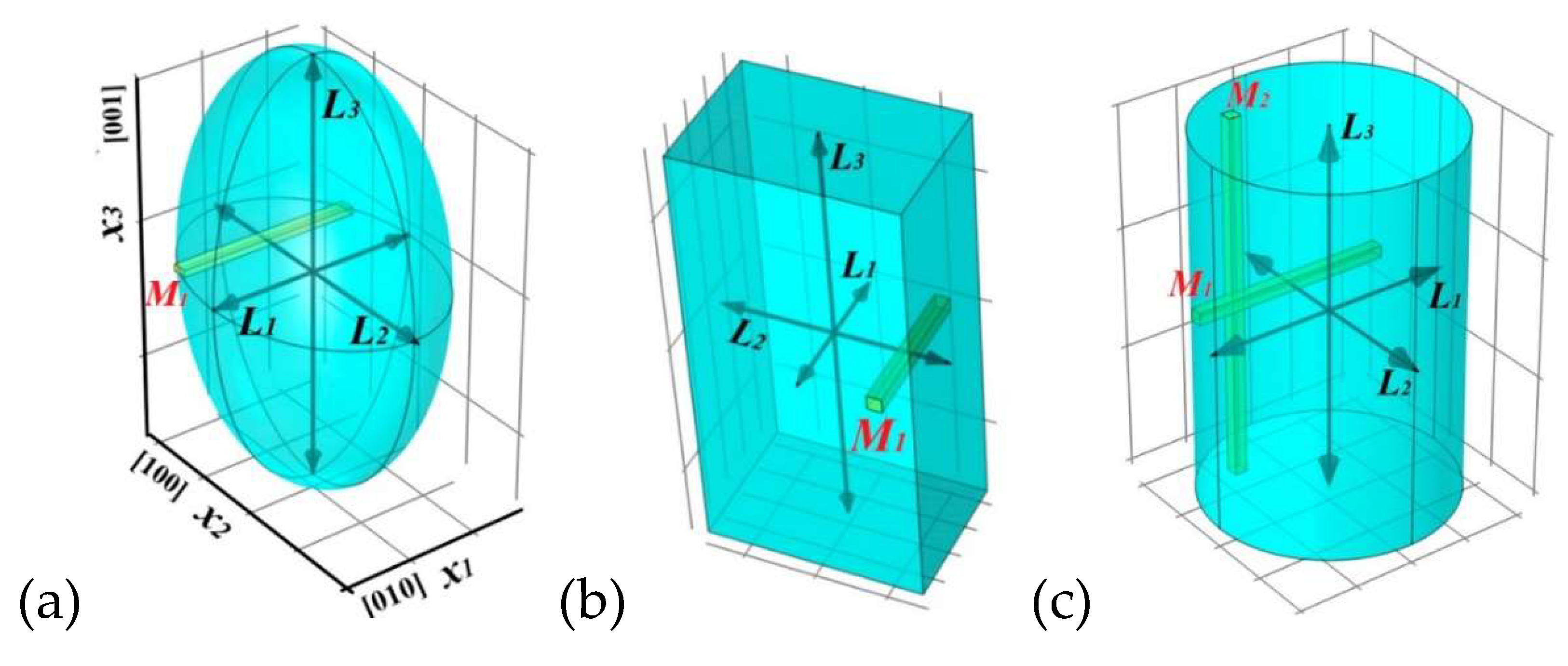
Figure 2.
(a) Histogram simulation of ellipsoid crystallite size distribution (g =2) along the [010] axis and its approximation by the dashed curve of the Lognormal distribution with the parameters: = 320 nm, = 0.5, r12 = r13 = r23 = r. Right axis - averaging over the columns in each histogram bin. (b) Histogram of distributions of X-ray diffraction sizes and the total value of histogram bars.
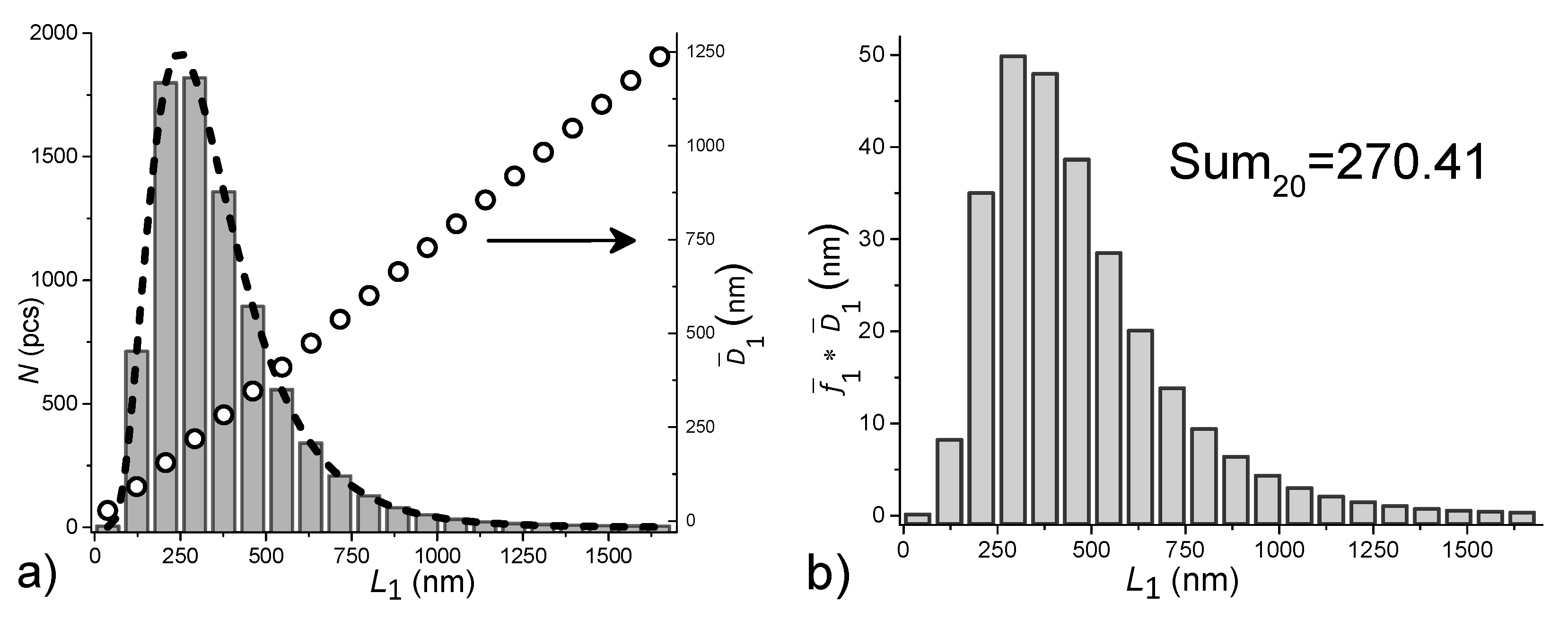
Figure 3.
Dependences of Kn on the correlation coefficients r and dispersion W1 of Lognormal distribution for ellipsoids g = 2 (a) and close to cuboids for g = 30 (b) using 20-bit histograms. For W1 = 0.6 calculations are shown using 30-bit histograms for W2 = W3 = 0.5 (o) and W2 = W3 = 0.7 (□).
Figure 3.
Dependences of Kn on the correlation coefficients r and dispersion W1 of Lognormal distribution for ellipsoids g = 2 (a) and close to cuboids for g = 30 (b) using 20-bit histograms. For W1 = 0.6 calculations are shown using 30-bit histograms for W2 = W3 = 0.5 (o) and W2 = W3 = 0.7 (□).
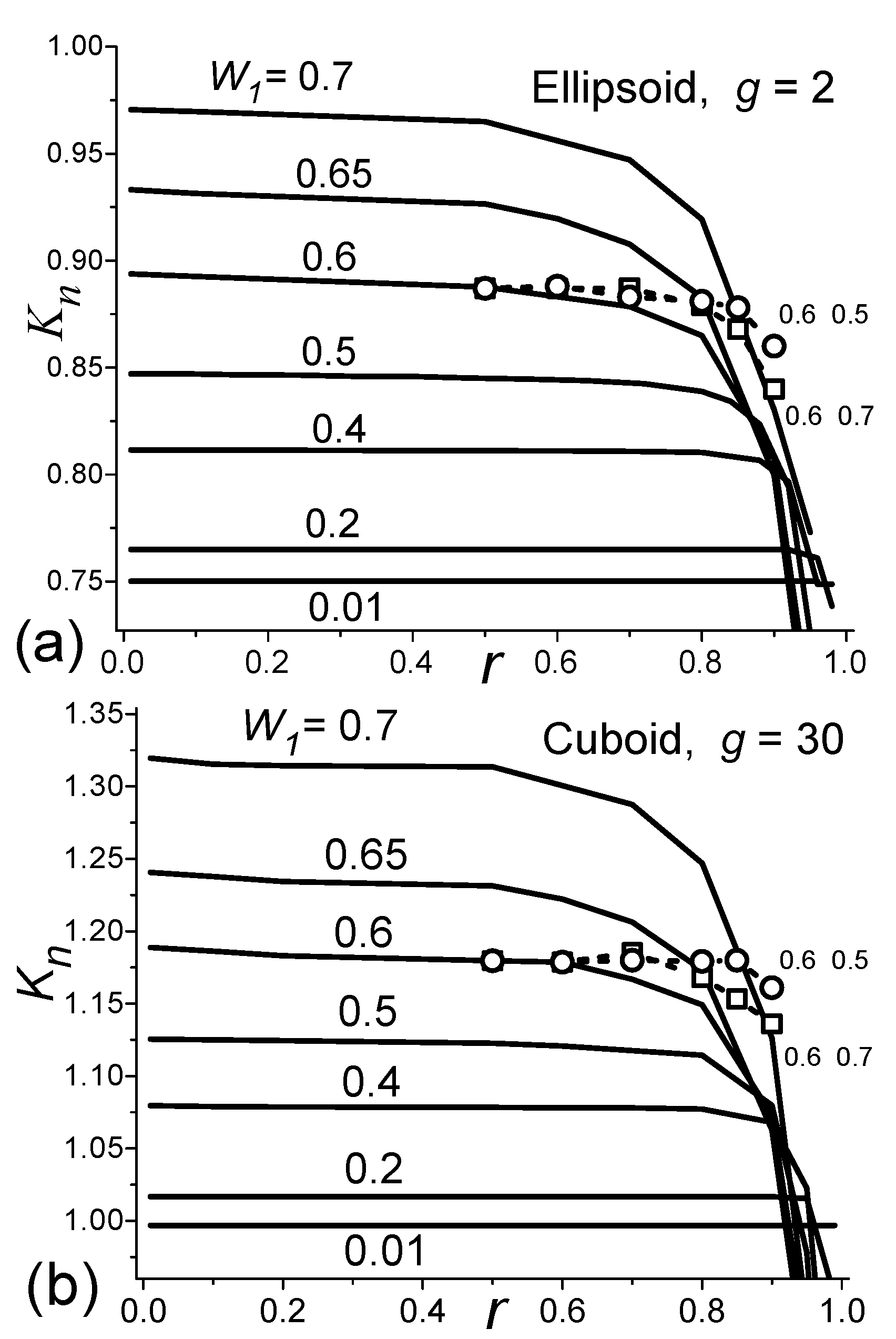
Figure 4.
Dependences of Kn on Lognormal dispersions W1 at r = 0.5 for ellipsoids (a) and cuboids (b) using 6-, 20- and 30-bit histograms: (■), (■) and (o), respectively. The red dot (■) is taken from SI. The straight line is an approximation by the equations shown in the figures.
Figure 4.
Dependences of Kn on Lognormal dispersions W1 at r = 0.5 for ellipsoids (a) and cuboids (b) using 6-, 20- and 30-bit histograms: (■), (■) and (o), respectively. The red dot (■) is taken from SI. The straight line is an approximation by the equations shown in the figures.
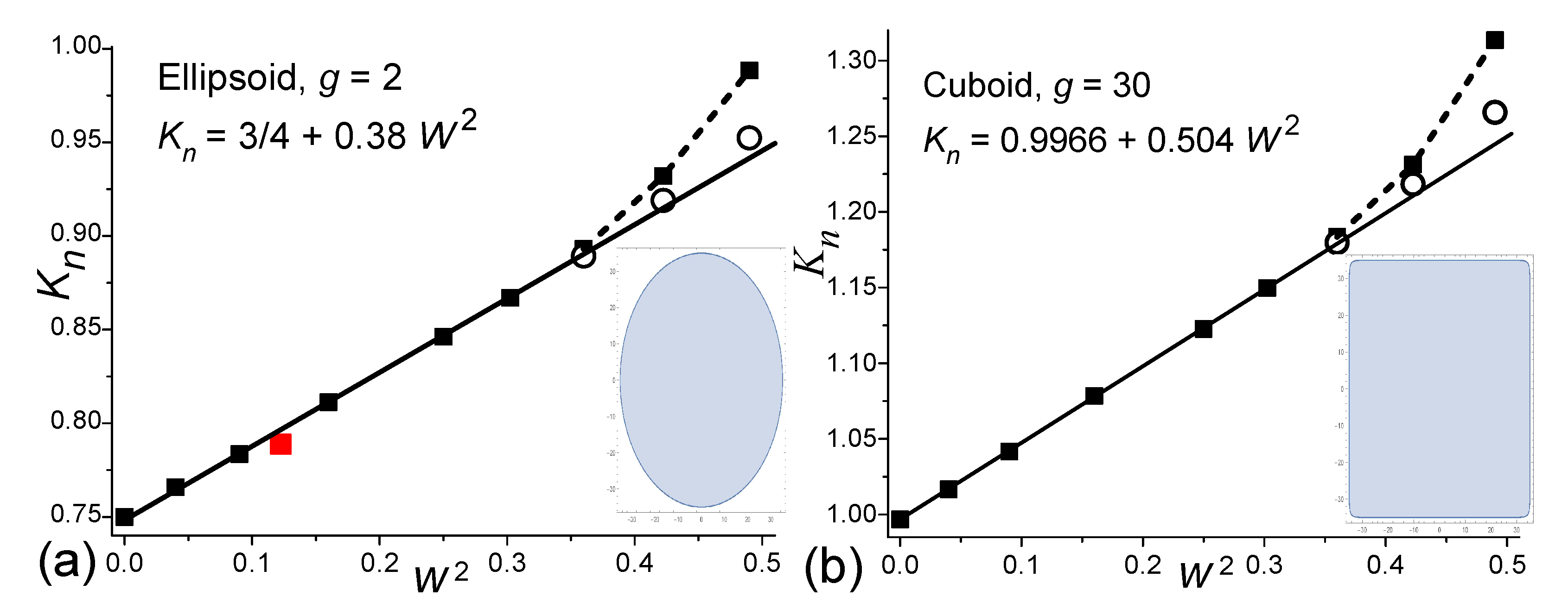
Figure 5.
Dependences of Kn on the correlation coefficient r and the dispersion W1 for ellipsoids (a) and bodies close to cuboids (b) using 20-bit Normal distribution histograms. For the solid lines - W1=W2 =W3. For W1 = 2 the calculations are shown for W2 =W3 =1.4 (o) and W2 =W3 =2.6 (□).
Figure 5.
Dependences of Kn on the correlation coefficient r and the dispersion W1 for ellipsoids (a) and bodies close to cuboids (b) using 20-bit Normal distribution histograms. For the solid lines - W1=W2 =W3. For W1 = 2 the calculations are shown for W2 =W3 =1.4 (o) and W2 =W3 =2.6 (□).
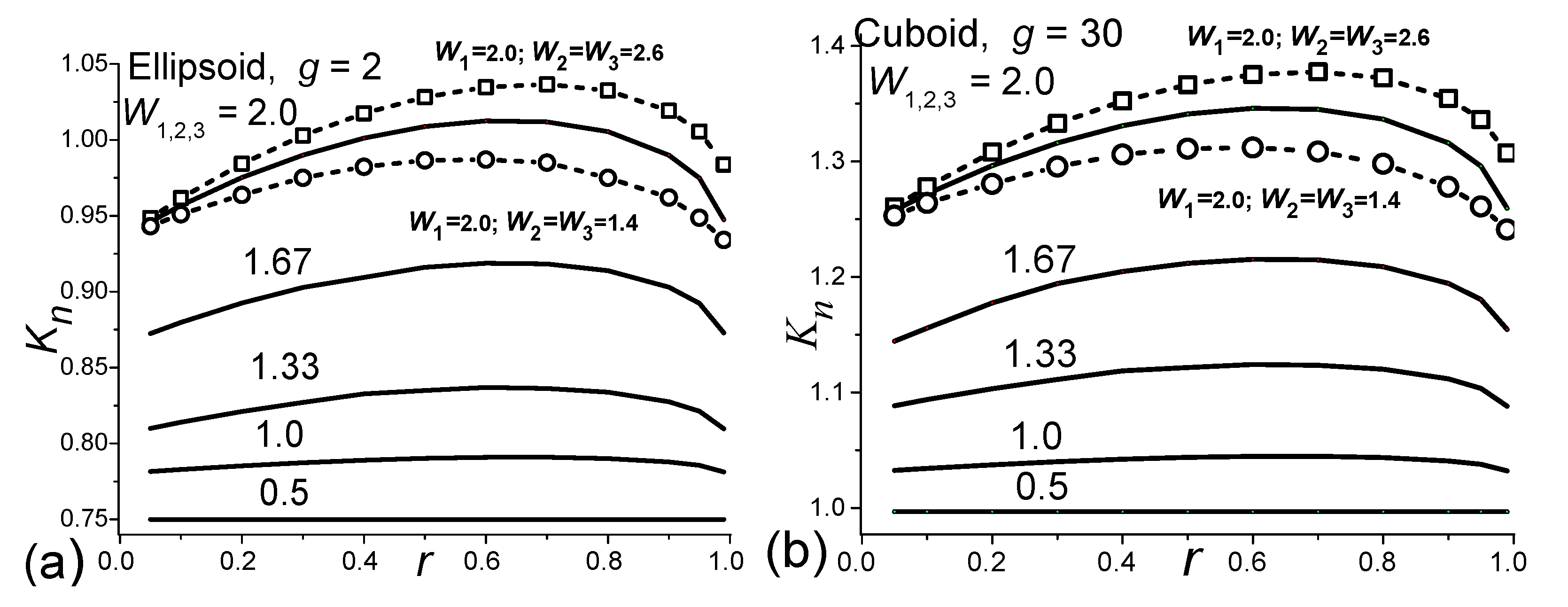
Figure 6.
Dependence of Kn on Normal dispersions W1 at r = 0.5 for ellipsoids (a) and cuboids (b) using 20-bit histograms, respectively, and dotted ends using 30-bit histograms. The figures show the relationships between the dispersions. The insets for the ratios W1=W2 =W3 show approximations by dotted lines on an enlarged scale. .
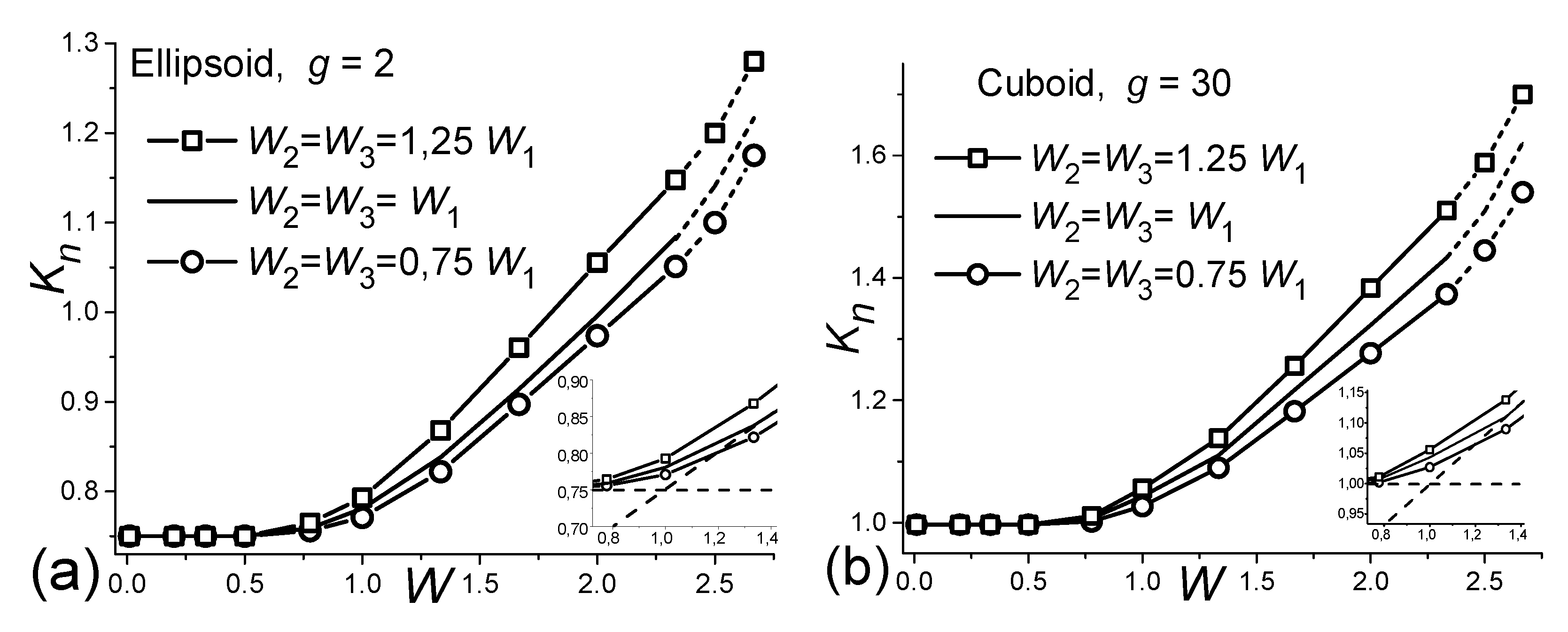

Table 1.
Equation (12) constants depending on the g-type superellipsoid shape.
| g | 2 | 4 | 6 | 8 | 10 | 30 | 50 |
| Kg,0 | 0.75 | 0.90 | 0.945 | 0.9654 | 0.9763 | 0.9966 | 0.9988 |
| Kg | 0.38 | 0.46 | 0.483 | 0.4938 | 0.4993 | 0.504 | 0.509 |
Disclaimer/Publisher’s Note: The statements, opinions and data contained in all publications are solely those of the individual author(s) and contributor(s) and not of MDPI and/or the editor(s). MDPI and/or the editor(s) disclaim responsibility for any injury to people or property resulting from any ideas, methods, instructions or products referred to in the content. |
© 2023 by the authors. Licensee MDPI, Basel, Switzerland. This article is an open access article distributed under the terms and conditions of the Creative Commons Attribution (CC BY) license (http://creativecommons.org/licenses/by/4.0/).
Copyright: This open access article is published under a Creative Commons CC BY 4.0 license, which permit the free download, distribution, and reuse, provided that the author and preprint are cited in any reuse.


